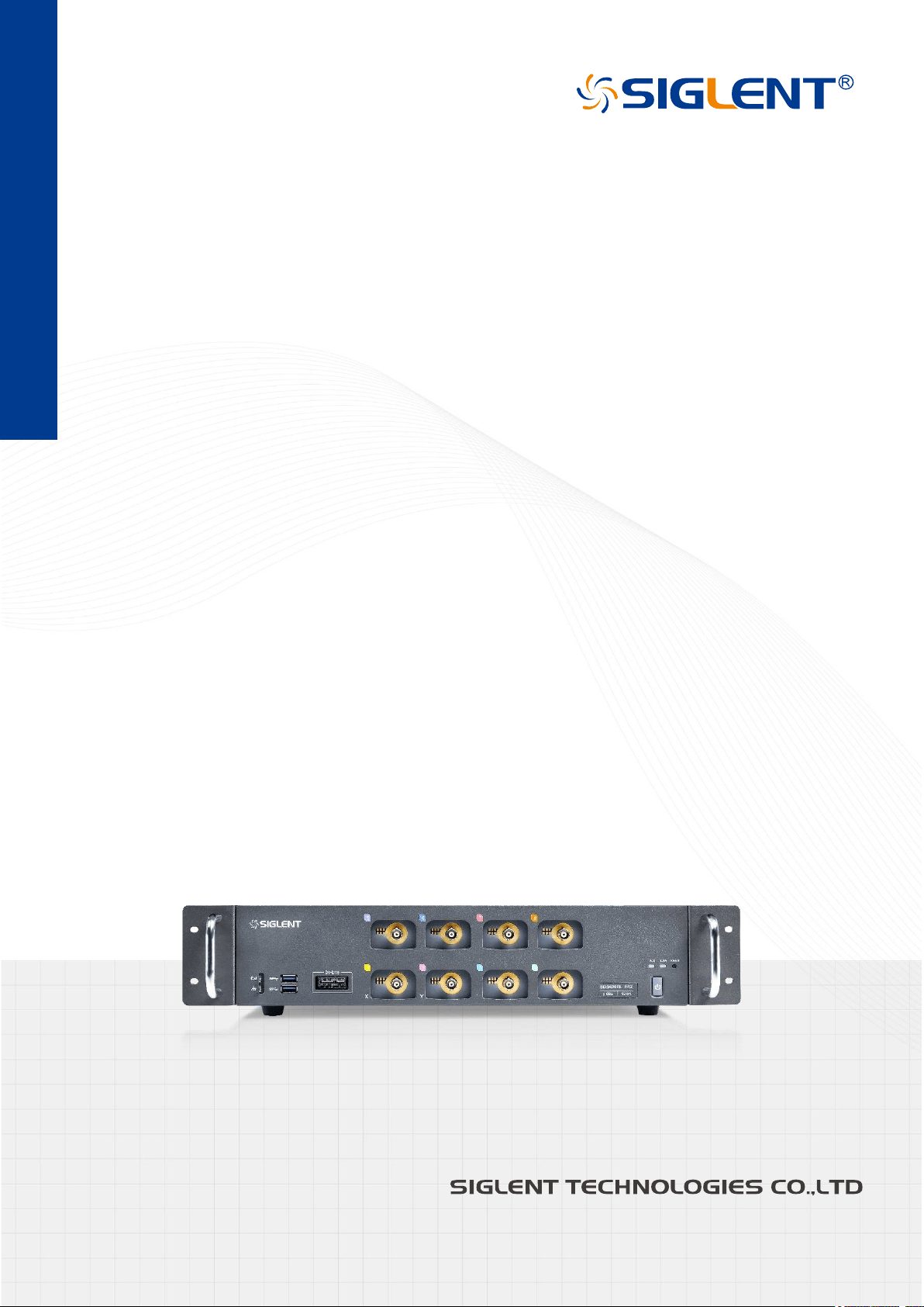
SDS6000L Series
Low Profile
Digital Oscilloscope
User Manual
EN01A


SDS6000L User Manual
i n t . s i g l e n t . c o m 1
Contents
CONTENTS ............................................................................................................................. 1
1 INTRODUCTION ................................................................................................................ 9
2 IMPORTANT SAFETY INFORMATION ............................................................................ 10
2.1 GENERAL SAFETY SUMMARY ................................................................................................... 10
2.2 SAFETY TERMS AND SYMBOLS ................................................................................................ 13
2.3 WORKING ENVIRONMENT ........................................................................................................ 14
2.4 COOLING REQUIREMENTS ....................................................................................................... 15
2.5 POWER AND GROUNDING REQUIREMENTS ............................................................................... 16
2.6 CLEANING ............................................................................................................................... 17
2.7 ABNORMAL CONDITIONS .......................................................................................................... 17
2.8 SAFETY COMPLIANCE .............................................................................................................. 18
INFORMATIONS ESSENTIELLES SUR LA SECURITE ....................................................... 19
EXIGENCE DE SECURITE ................................................................................................................... 19
TERMES ET SYMBOLES DE SECURITE ................................................................................................. 21
ENVIRONNEMENT DE TRAVAIL ............................................................................................................ 22
EXIGENCES DE REFROIDISSEMENT .................................................................................................... 24
CONNEXIONS D'ALIMENTATION ET DE TERRE ...................................................................................... 24
NETTOYAGE ..................................................................................................................................... 25
CONDITIONS ANORMALES.................................................................................................................. 26
CONFORMITE EN MATIERE DE SECURITE ............................................................................................ 26
3 FIRST STEPS .................................................................................................................. 27
3.1 DELIVERY CHECKLIST ............................................................................................................. 27
3.2 QUALITY ASSURANCE .............................................................................................................. 27
3.3 MAINTENANCE AGREEMENT .................................................................................................... 27
4 DOCUMENT CONVENTIONS .......................................................................................... 28
5 GETTING STARTED ........................................................................................................ 29
5.1 MECHANICAL DIMENSION ........................................................................................................ 29
5.2 FRONT PANEL OVERVIEW ........................................................................................................ 30
5.3 REAR PANEL OVERVIEW .......................................................................................................... 31
5.4 TO INSTALL THE RACKMOUNT FLANGE KIT ............................................................................... 32
5.5 CONNECTING TO EXTERNAL DEVICES/SYSTEMS ....................................................................... 32
5.5.1 Power Supply ........................................................................................................................ 32
5.5.2 Probes ................................................................................................................................... 32
5.5.3 LAN ....................................................................................................................................... 34
5.5.4 External Monitor and Mouse ................................................................................................. 34
5.5.5 Auxiliary Output ..................................................................................................................... 34

SDS6000L User Manual
2 i n t . s i g l e n t . c o m
5.5.6 Reference Input and Output .................................................................................................. 35
5.5.7 Waveform Generator ............................................................................................................. 35
5.5.8 Logic Probe ........................................................................................................................... 35
5.6 POWER ON ............................................................................................................................. 36
5.7 SHUT DOWN ............................................................................................................................ 36
5.8 SYSTEM INFORMATION ............................................................................................................ 37
5.9 INSTALL OPTIONS .................................................................................................................... 37
6 REMOTE CONTROL ....................................................................................................... 38
6.1 WEB BROWSER ...................................................................................................................... 38
6.2 OTHER CONNECTIVITY ............................................................................................................ 39
7 SCREEN DISPLAY .......................................................................................................... 40
7.1 OVERVIEW .............................................................................................................................. 40
7.2 MENU BAR .............................................................................................................................. 41
7.3 GRID AREA ............................................................................................................................. 41
7.4 CHANNEL DESCRIPTOR BOX .................................................................................................... 43
7.5 TIMEBASE AND TRIGGER DESCRIPTOR BOXES ......................................................................... 44
7.6 DIALOG BOX ........................................................................................................................... 47
7.7 MOUSE CONTROL ................................................................................................................... 49
7.8 CHOOSING THE LANGUAGE...................................................................................................... 50
8 MULTIPLE APPROACHES TO RECALL FUNCTIONS ................................................... 51
8.1 MENU BAR .............................................................................................................................. 51
8.2 DESCRIPTOR BOX ................................................................................................................... 51
9 VERTICAL SETUP .......................................................................................................... 52
9.1 TURN ON/OFF A CHANNEL ........................................................................................................ 52
9.2 CHANNEL SETUP ..................................................................................................................... 53
10 DIGITAL CHANNELS ...................................................................................................... 60
10.1 OVERVIEW .............................................................................................................................. 60
10.2 ENABLE/DISABLE THE DIGITAL CHANNELS ................................................................................ 61
10.3 DIGITAL CHANNEL SETUP ........................................................................................................ 62
11 HORIZONTAL AND ACQUISITION SETUP ..................................................................... 66
11.1 TIMEBASE SETUP .................................................................................................................... 66
11.2 ACQUISITION SETUP ................................................................................................................ 67
11.2.1 Overview ............................................................................................................................... 67
11.2.2 Acquisition ............................................................................................................................. 69
11.2.3 Memory Management ........................................................................................................... 72
11.2.4 Roll Mode .............................................................................................................................. 73
11.2.5 Sequence .............................................................................................................................. 73
11.2.6 ESR ....................................................................................................................................... 76
11.3 HISTORY ................................................................................................................................. 80

SDS6000L User Manual
i n t . s i g l e n t . c o m 3
12 ZOOM .............................................................................................................................. 83
13 TRIGGER ......................................................................................................................... 85
13.1 OVERVIEW .............................................................................................................................. 85
13.2 TRIGGER SETUP ..................................................................................................................... 86
13.3 TRIGGER LEVEL ...................................................................................................................... 87
13.4 TRIGGER MODE ...................................................................................................................... 88
13.5 TRIGGER TYPE........................................................................................................................ 89
13.5.1 Overview ............................................................................................................................... 89
13.5.2 Edge Trigger .......................................................................................................................... 90
13.5.3 Slope Trigger ......................................................................................................................... 90
13.5.4 Pulse Trigger ......................................................................................................................... 92
13.5.5 Video Trigger ......................................................................................................................... 94
13.5.6 Window Trigger ..................................................................................................................... 98
13.5.7 Interval Trigger ...................................................................................................................... 99
13.5.8 Dropout Trigger ................................................................................................................... 100
13.5.9 Runt Trigger ........................................................................................................................ 101
13.5.10 Pattern Trigger .................................................................................................................... 101
13.5.11 Qualified Trigger .................................................................................................................. 103
13.5.12 Nth Edge Trigger ................................................................................................................. 104
13.5.13 Delay Trigger ....................................................................................................................... 105
13.5.14 Setup/Hold Trigger .............................................................................................................. 105
13.5.15 Serial Trigger ....................................................................................................................... 106
13.6 TRIGGER SOURCE ................................................................................................................. 106
13.7 HOLDOFF .............................................................................................................................. 107
13.8 TRIGGER COUPLING .............................................................................................................. 108
13.9 NOISE REJECT ...................................................................................................................... 109
13.10 ZONE TRIGGER ..................................................................................................................... 110
14 SERIAL TRIGGER AND DECODE ................................................................................ 115
14.1 OVERVIEW ............................................................................................................................ 115
14.2 I2C TRIGGER AND SERIAL DECODE ....................................................................................... 117
14.2.1 I2C Signal Settings.............................................................................................................. 117
14.2.2 I2C Trigger .......................................................................................................................... 118
14.2.3 I2C Serial Decode ............................................................................................................... 122
14.3 SPI TRIGGER AND SERIAL DECODE ....................................................................................... 125
14.3.1 SPI Signal Settings ............................................................................................................. 125
14.3.2 SPI Trigger .......................................................................................................................... 128
14.3.3 SPI Serial Decode ............................................................................................................... 128
14.4 UART TRIGGER AND SERIAL DECODE ................................................................................... 129
14.4.1 UART Signal Settings ......................................................................................................... 129

SDS6000L User Manual
4 i n t . s i g l e n t . c o m
14.4.2 UART Trigger ...................................................................................................................... 130
14.4.3 UART Serial Decode ........................................................................................................... 130
14.5 CAN TRIGGER AND SERIAL DECODE ..................................................................................... 131
14.5.1 CAN Signal Settings............................................................................................................ 131
14.5.2 CAN Trigger ........................................................................................................................ 131
14.5.3 CAN Serial Decode ............................................................................................................. 132
14.6 LIN TRIGGER AND SERIAL DECODE ....................................................................................... 134
14.6.1 LIN Signal Settings.............................................................................................................. 134
14.6.2 LIN Trigger .......................................................................................................................... 134
14.6.3 LIN Serial Decode ............................................................................................................... 135
14.7 FLEXRAY TRIGGER AND SERIAL DECODE ............................................................................... 136
14.7.1 FlexRay Signal Settings ...................................................................................................... 136
14.7.2 FlexRay Trigger ................................................................................................................... 136
14.7.3 FlexRay Serial Decode ....................................................................................................... 137
14.8 CAN FD TRIGGER AND SERIAL DECODE ................................................................................ 139
14.8.1 CAN FD Signal Settings ...................................................................................................... 139
14.8.2 CAN FD Trigger ................................................................................................................... 139
14.8.3 CAN FD Serial Decode ....................................................................................................... 140
14.9 I2S TRIGGER AND SERIAL DECODE ........................................................................................ 142
14.9.1 I2S Signal Settings .............................................................................................................. 142
14.9.2 I2S Trigger ........................................................................................................................... 143
14.9.3 I2S Serial Decode ............................................................................................................... 144
14.10 MIL-STD-1553B TRIGGER AND SERIAL DECODE ................................................................... 145
14.10.1 MIL-STD-1553B Signal Settings ......................................................................................... 145
14.10.2 MIL-STD-1553B Serial Decode .......................................................................................... 145
14.11 SENT TRIGGER AND SERIAL DECODE ................................................................................... 146
14.11.1 SENT Signal Settings.......................................................................................................... 146
14.11.2 SENT Trigger ...................................................................................................................... 147
14.11.3 SENT Serial Decode ........................................................................................................... 150
14.12 MANCHESTER SERIAL DECODE ............................................................................................. 151
14.12.1 Manchester Signal Settings ................................................................................................ 152
14.12.2 Manchester Serial Decode .................................................................................................. 153
15 CURSORS ..................................................................................................................... 154
15.1 OVERVIEW ............................................................................................................................ 154
15.2 SELECT AND MOVE CURSORS ............................................................................................... 160
16 MEASUREMENT ........................................................................................................... 162
16.1 OVERVIEW ............................................................................................................................ 162
16.2 SET PARAMETERS ................................................................................................................. 163
16.3 TYPE OF MEASUREMENT ....................................................................................................... 166

SDS6000L User Manual
i n t . s i g l e n t . c o m 5
16.3.1 Vertical Measurement ......................................................................................................... 166
16.3.2 Horizontal Measurement ..................................................................................................... 168
16.3.3 Miscellaneous Measurements ............................................................................................ 169
16.3.4 Delay Measurement ............................................................................................................ 170
16.4 TREND .................................................................................................................................. 171
16.5 TRACK .................................................................................................................................. 172
16.6 DISPLAY MODE ..................................................................................................................... 173
16.7 MEASUREMENT STATISTICS ................................................................................................... 174
16.8 STATISTICS HISTOGRAM ........................................................................................................ 175
16.9 SIMPLE MEASUREMENTS ....................................................................................................... 176
16.10 GATE .................................................................................................................................... 177
16.11 AMPLITUDE STRATEGY .......................................................................................................... 178
16.12 THRESHOLD .......................................................................................................................... 178
16.13 HARDWARE FREQUENCY COUNTER ....................................................................................... 179
17 MATH ............................................................................................................................. 180
17.1 OVERVIEW ............................................................................................................................ 180
17.2 ARITHMETIC .......................................................................................................................... 181
17.2.1 Addition / Subtraction / Multiplication / Division .................................................................. 181
17.2.2 Identity / Negation ............................................................................................................... 182
17.2.3 Average / ERES .................................................................................................................. 183
17.2.4 Max-hold / Min-hold............................................................................................................. 183
17.3 ALGEBRA .............................................................................................................................. 183
17.3.1 Differential ........................................................................................................................... 183
17.3.2 Integral ................................................................................................................................ 184
17.3.3 Square Root ........................................................................................................................ 185
17.3.4 Absolute .............................................................................................................................. 186
17.3.5 Sign ..................................................................................................................................... 186
17.3.6 exp/exp10 ............................................................................................................................ 187
17.3.7 ln/lg ...................................................................................................................................... 187
17.3.8 Interpolate ........................................................................................................................... 188
17.4 FILTER .................................................................................................................................. 188
17.5 FREQUENCY ANALYSIS .......................................................................................................... 190
17.6 FORMULA EDITOR ................................................................................................................. 198
18 REFERENCE ................................................................................................................. 200
19 MEMORY ....................................................................................................................... 202
20 SEARCH ........................................................................................................................ 204
21 NAVIGATE ..................................................................................................................... 207
22 MASK TEST .................................................................................................................. 212
22.1 OVERVIEW ............................................................................................................................ 212

SDS6000L User Manual
6 i n t . s i g l e n t . c o m
22.2 MASK SETUP ........................................................................................................................ 214
22.2.1 Create Mask ........................................................................................................................ 214
22.2.2 Mask Editor ......................................................................................................................... 215
22.3 PASS/FAIL RULE ................................................................................................................... 217
22.4 OPERATION ........................................................................................................................... 217
23 DVM ............................................................................................................................... 218
23.1 OVERVIEW ............................................................................................................................ 218
23.2 MODE ................................................................................................................................... 219
23.3 DIAGRAMS ............................................................................................................................ 220
24 COUNTER ..................................................................................................................... 223
24.1 OVERVIEW ............................................................................................................................ 223
24.2 MODE ................................................................................................................................... 225
25 HISTOGRAM ................................................................................................................. 226
25.1 OVERVIEW ............................................................................................................................ 226
25.2 REGION SETTING .................................................................................................................. 228
26 POWER ANALYSIS ....................................................................................................... 230
26.1 OVERVIEW ............................................................................................................................ 230
26.2 POWER QUALITY ................................................................................................................... 230
26.3 CURRENT HARMONICS .......................................................................................................... 233
26.4 INRUSH CURRENT ................................................................................................................. 235
26.5 SWITCHING LOSS .................................................................................................................. 236
26.6 SLEW RATE ........................................................................................................................... 239
26.7 MODULATION ........................................................................................................................ 240
26.8 OUTPUT RIPPLE .................................................................................................................... 240
26.9 TURN ON/TURN OFF ............................................................................................................. 241
26.10 TRANSIENT RESPONSE.......................................................................................................... 242
26.11 PSRR .................................................................................................................................. 244
26.12 POWER EFFICIENCY .............................................................................................................. 245
26.13 SOA ..................................................................................................................................... 245
27 BODE PLOT .................................................................................................................. 248
27.1 OVERVIEW ............................................................................................................................ 248
27.2 CONFIGURATION ................................................................................................................... 249
27.2.1 Connection .......................................................................................................................... 249
27.2.2 Sweep ................................................................................................................................. 249
27.3 DISPLAY ................................................................................................................................ 252
27.4 DATA ANALYSIS ..................................................................................................................... 254
28 EYE DIAGRAM .............................................................................................................. 257
28.1 OVERVIEW ............................................................................................................................ 257

SDS6000L User Manual
i n t . s i g l e n t . c o m 7
28.2 SIGNAL SETTING ................................................................................................................... 259
28.3 CLOCK RECOVERY ................................................................................................................ 260
28.4 MEASUREMENT ..................................................................................................................... 261
28.5 MASK TEST ........................................................................................................................... 263
28.6 OTHER OPERATION ............................................................................................................... 263
29 JITTER ANALYSIS ........................................................................................................ 264
29.1 OVERVIEW ............................................................................................................................ 264
29.2 SIGNAL CONFIGURATION ....................................................................................................... 265
29.3 CLOCK RECOVERY ................................................................................................................ 266
29.4 JITTER DECOMPOSITION ........................................................................................................ 266
29.5 JITTER MEASURE .................................................................................................................. 267
29.6 OTHER OPERATION ............................................................................................................... 270
29.7 SYSTEM EFFECT ON JITTER MEASURE ................................................................................... 270
30 DISPLAY ........................................................................................................................ 271
31 WAVEFORM GENERATOR ........................................................................................... 279
31.1 OVERVIEW ............................................................................................................................ 279
31.2 WAVE TYPE .......................................................................................................................... 280
31.3 OTHER SETTING ................................................................................................................... 281
31.4 SYSTEM ................................................................................................................................ 282
32 SAVE/RECALL .............................................................................................................. 284
32.1 SAVE TYPE ........................................................................................................................... 284
32.2 FILE MANAGER ..................................................................................................................... 287
32.3 SAVE AND RECALL INSTANCES ............................................................................................... 288
33 UTILITY ......................................................................................................................... 292
33.1 SYSTEM INFORMATION .......................................................................................................... 292
33.2 SYSTEM SETTING .................................................................................................................. 292
33.2.1 Language ............................................................................................................................ 292
33.2.2 Screen Saver ...................................................................................................................... 293
33.2.3 Sound .................................................................................................................................. 293
33.2.4 Auto Power-on .................................................................................................................... 293
33.2.5 Date/Time ............................................................................................................................ 293
33.2.6 Reference Position Setting ................................................................................................. 294
33.2.7 Tips...................................................................................................................................... 297
33.3 I/O SETTING ......................................................................................................................... 297
33.3.1 LAN ..................................................................................................................................... 297
33.3.2 Clock Source ....................................................................................................................... 298
33.4 INSTALL OPTIONS .................................................................................................................. 299
33.5 MAINTENANCE ...................................................................................................................... 300
33.5.1 Upgrade .............................................................................................................................. 300

SDS6000L User Manual
8 i n t . s i g l e n t . c o m
33.5.2 Self-Calibration .................................................................................................................... 301
33.5.3 Developer Options .............................................................................................................. 302
33.6 SERVICE ............................................................................................................................... 302
33.6.1 Web ..................................................................................................................................... 302
33.6.2 Network Mapping ................................................................................................................ 302
33.6.3 Emulation ............................................................................................................................ 303
33.6.4 LXI ....................................................................................................................................... 304
33.6.5 Share File ............................................................................................................................ 305
34 TROUBLESHOOTING ................................................................................................... 306

SDS6000L User Manual
i n t . s i g l e n t . c o m 9
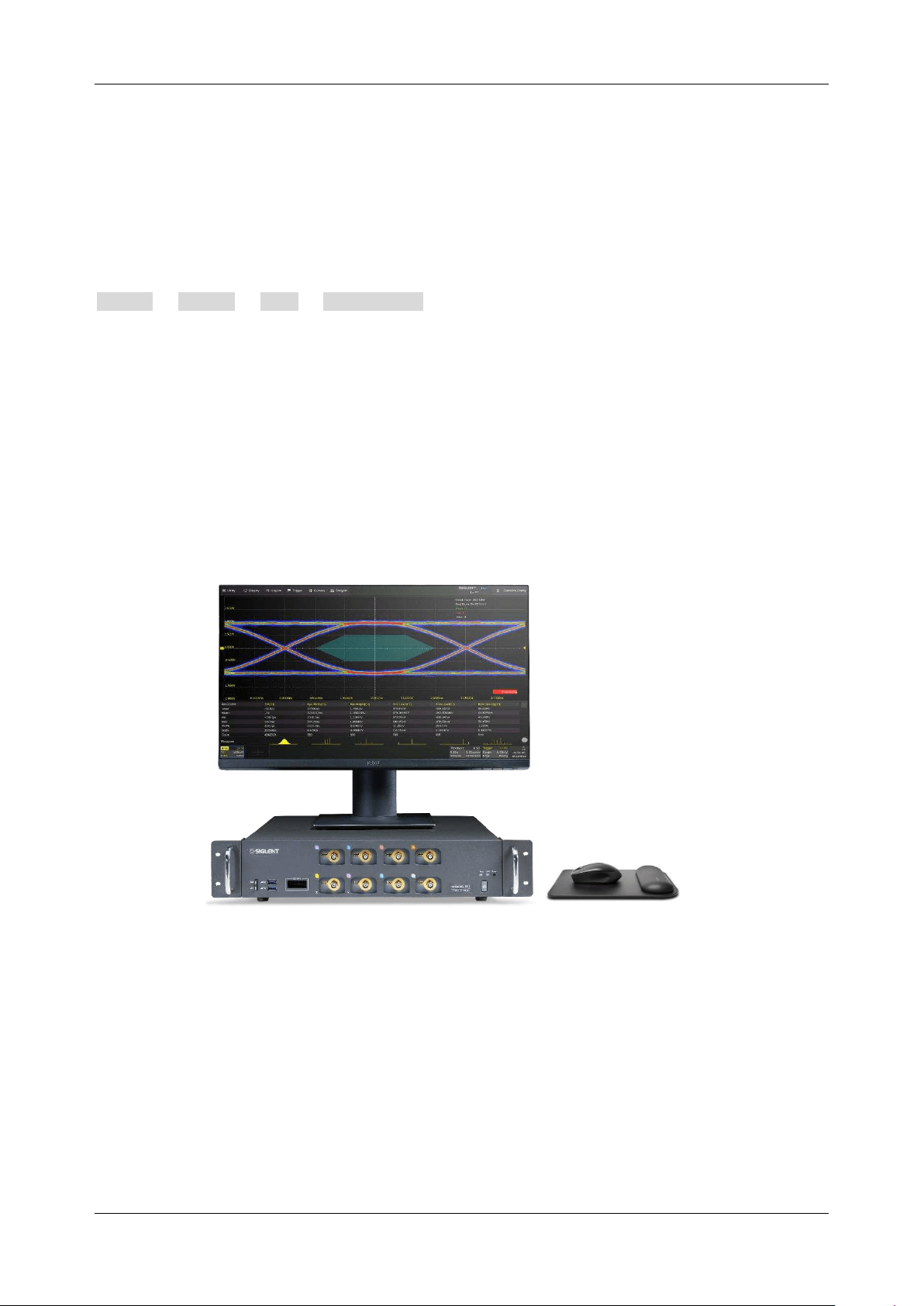
1 Introduction
A digital oscilloscope is a multi-functional instrument for displaying, analyzing, and storing electrical
signals. It is an indispensable tool for designing, manufacturing, and maintaining electronic equipment.
This user manual includes important safety and installation information related to the SDS6000L series
of low-profile oscilloscopes and includes simple tutorials for the basic operation of the instrument.
The series includes the following models:
Model
Analog
Bandwidth
Maximum Sampling Rate
Analog
Channels
SDS6208L
2 GHz
5 GSa/s (10 GSa/s ESR)
@ each channel
8
SDS6204L
2 GHz
5 GSa/s (10 GSa/s ESR)
@ each channel
4
SDS6108L
1 GHz
5 GSa/s (10 GSa/s ESR)
@ each channel
8
SDS6104L
1 GHz
5 GSa/s (10 GSa/s ESR)
@ each channel
4
SDS6058L
500 MHz
5 GSa/s (10 GSa/s ESR)
@ each channel
8
SDS6054L
500 MHz
5 GSa/s (10 GSa/s ESR)
@ each channel
4

SDS6000L User Manual
10 i n t . s i g l e n t . c o m
2 Important Safety Information
This manual contains information and warnings that must be followed by the user for safe operation
and to keep the product in a safe condition.
2.1 General Safety Summary
Carefully read the following safety precautions to avoid personal injury and prevent damage to the
instrument and any products connected to it. To avoid potential hazards, please use the instrument as
specified.
To Avoid Fire or Personal Injury.
Use the Proper Power Line.
Only use a local / state-approved power cord for connecting the instrument to mains power sources.
Ground the Instrument.
The instrument grounds through the protective terra conductor of the power line. To avoid electric
shock, the ground conductor must be connected to the earth. Make sure the instrument is grounded
correctly before connecting its input or output terminals.
Connect the Signal Wire Correctly.
The potential of the signal wire is equal to the earth, so do not connect the signal wire to a high voltage.
Do not touch the exposed contacts or components.
Look over All Terminals’ Ratings.
To avoid fire or electric shock, please look over all ratings and signed instructions of the instrument.
Before connecting the instrument, please read the manual carefully to gain more information about the
ratings.
Equipment Maintenance and Service.
When the equipment fails, please do not dismantle the machine for maintenance. The equipment

SDS6000L User Manual
int. s i g l e n t . c o m 11
contains capacitors, power supply, transformers, and other energy storage devices, which may cause
high voltage damage. The internal devices of the equipment are sensitive to static electricity, and direct
contact can easily cause irreparable damage to the equipment. It is necessary to return to the factory
or the company's designated maintenance organization for maintenance. Be sure to pull out the power
supply when repairing the equipment. Live line operation is strictly prohibited. The equipment can only
be powered on when the maintenance is completed and the maintenance is confirmed to be successful.
Identification of Normal State of Equipment.
After the equipment is started, there will be no alarm information or error information at the interface
under normal conditions. If there is a pop-up window or button during the scanning process or there is
an alarm or error prompt, the device may be in an abnormal state. You need to view the specific prompt
information. You can try to restart the instrument to see if it corrects the error condition. If the fault
information is still in place, do not use the instrument for testing. Contact the manufacturer or the
maintenance department designated by the manufacturer to carry out maintenance before reusing the
product.
Not Operate with Suspected Failures.
If you suspect that there is damage to the instrument, please let qualified service personnel check it.
Avoid Circuit or Wire Exposed Components Exposed.
Do not touch exposed contacts or components when the power is on.
Do not operate in wet/damp conditions.
Do not operate in an explosive atmosphere.
Keep the surface of the instrument clean and dry.
Only probe assemblies that meet the requirement of UL61010-031 and CAN/CSA-C22.2
No.61010-031 shall be used.
Only a lithium battery with the same specifications as the original battery should be used to

SDS6000L User Manual
12 i n t . s i g l e n t . c o m
replace the battery on the mainboard.
Do not use the equipment for measurements on mains circuits. Do not use the equipment for
measurements on voltages exceeding the voltage ranges described in the manual. The
maximum additional transient voltage cannot exceed 1300 V.
The responsible body or operator should refer to the instruction manual to preserve the
protection afforded by the equipment. If the equipment is used in a manner not specified by the
manufacturer, the protection provided by the equipment may be impaired.
Any parts of the device and its accessories are not allowed to be changed or replaced, other
than authorized by the manufacturer or agent.
SDS6000L User Manual
int. s i g l e n t . c o m 13
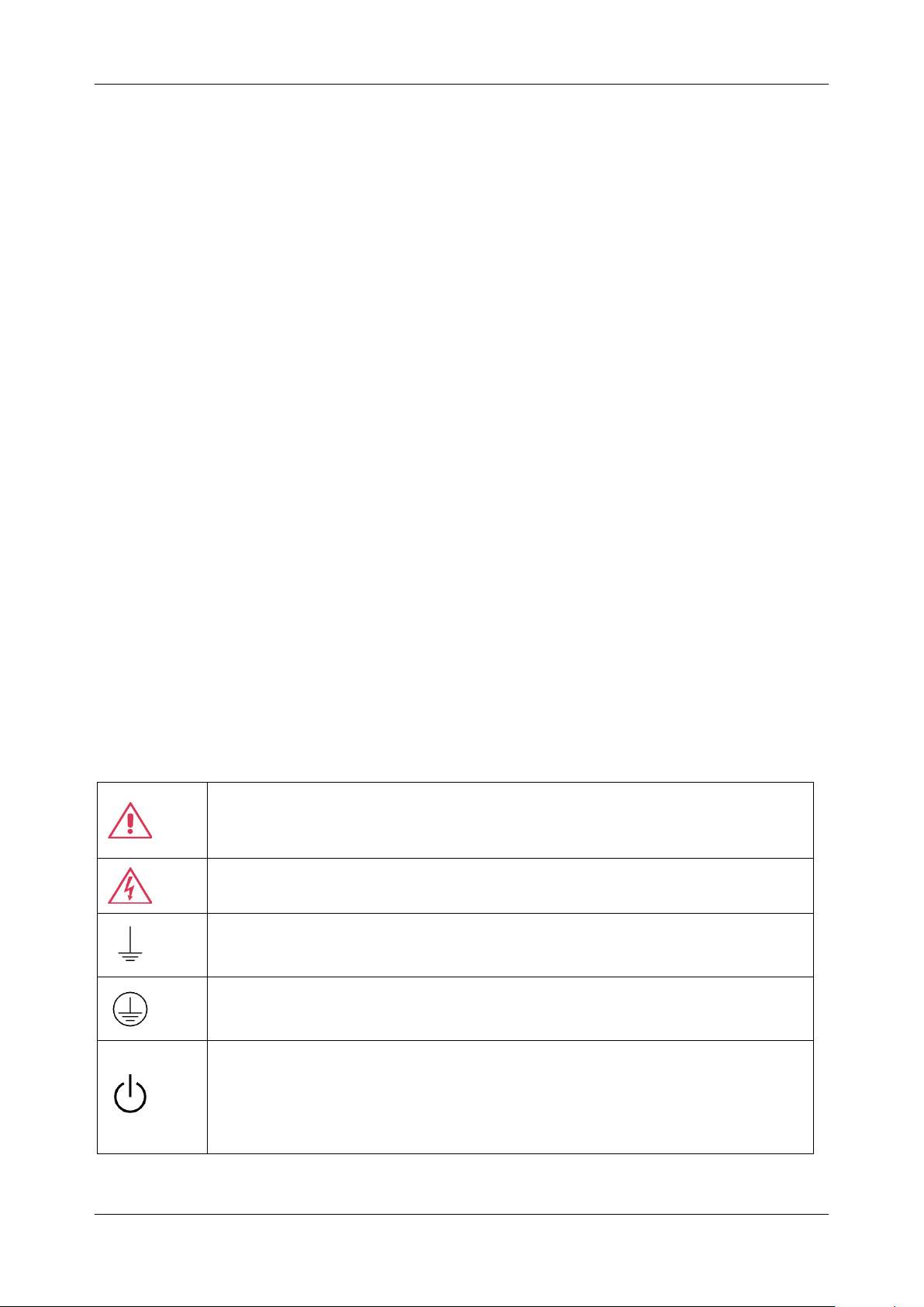
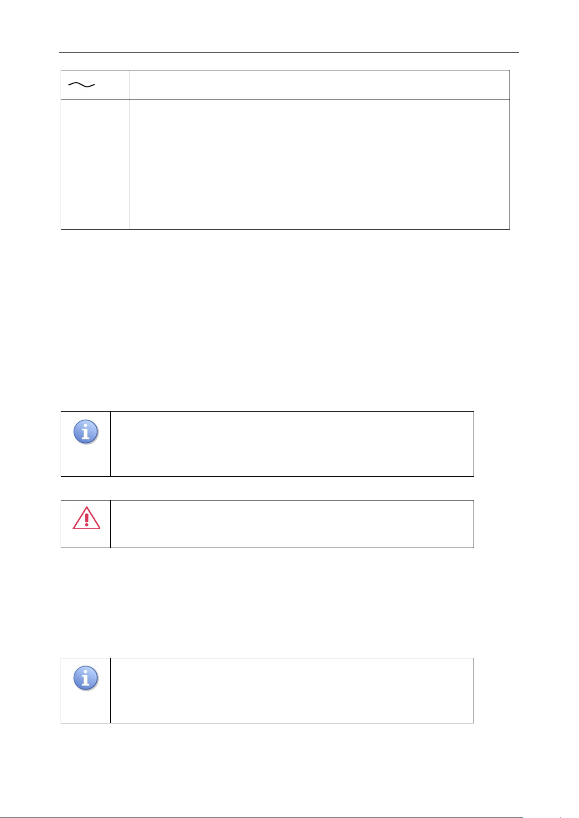
2.2 Safety Terms and Symbols
When the following symbols or terms appear on the front or rear panel of the instrument or in this
manual, they indicate special care in terms of safety.
This symbol is used where caution is required. Refer to the accompanying
information or documents to protect against personal injury or damage to the
instrument.
This symbol warns of a potential risk of shock hazard.
This symbol is used to denote the measurement ground connection.
This symbol is used to denote a safety ground connection.
This symbol shows that the switch is an On/Standby switch. When it is pressed,
the scope’s state switches between Operation and Standby. This switch does not
disconnect the device's power supply. To completely power off the scope, the
power switch on the rear panel should be turned to “Off”.
This symbol is used to represent alternating current, or "AC".
CAUTION
The "CAUTION" symbol indicates a potential hazard. It calls attention to a
procedure, practice, or condition which may be dangerous if not followed. Do not
proceed until its conditions are fully understood and met.
WARNING
The "WARNING" symbol indicates a potential hazard. It calls attention to a
procedure, practice, or condition which, if not followed, could cause bodily injury
or death. If a WARNING is indicated, do not proceed until the safety conditions
are fully understood and met.
SDS6000L User Manual
14 i n t . s i g l e n t . c o m
2.3 Working Environment
The design of the instrument has been verified to conform to EN 61010-1 safety standard per the
following limits:
Environment
The instrument is used indoors and should be operated in a clean and dry environment with an ambient
temperature range.
Note:
Direct sunlight, electric heaters, and other heat sources should be
considered when evaluating the ambient temperature.
Warning
: Do not operate the instrument in explosive, dusty, or humid
environments.
Ambient Temperature
Operating: 0
℃
to +50
℃
Non-operation: -30
℃
to +70
℃
Note:
Direct sunlight, radiators, and other heat sources should be taken into
account when assessing the ambient temperature.
Humidity
Operating: 5% ~ 90% RH, 30
℃
, derate to 50% RH at 40
℃
Non-operating: 5% ~ 95% RH
Altitude
Operating: ≤ 3,048 m, 25
℃
Non-operating: ≤ 12,191 m
SDS6000L User Manual
int. s i g l e n t . c o m 15
Installation (overvoltage) Category
This product is powered by mains conforming to installation (overvoltage) Category II.
Note:
Installation (overvoltage) category I refers to situations where
equipment measurement terminals are connected to the source circuit. In
these terminals, precautions are done to limit the transient voltage to a
correspondingly low level.
Installation (overvoltage) category II refers to the local power distribution level
which applies to equipment connected to the AC line (AC power).
Degree of Pollution
The oscilloscopes may be operated in environments of Pollution Degree II.
Note:
Degree of Pollution II refers to a working environment that is dry and
non-conductive pollution occurs. Occasional temporary conductivity caused
by condensation is expected.
IP Rating
IP20 (as defined in IEC 60529).
2.4 Cooling Requirements
This instrument relies on forced air cooling with internal fans and ventilation openings. Care must be
taken to avoid restricting the airflow around the apertures (fan holes) on each side of the scope. To
ensure adequate ventilation it is required to leave a 15 cm (6 inch) minimum gap around the sides of
the instrument.
CAUTION:
Do not block the ventilation holes located on both sides of the
scope.
SDS6000L User Manual
16 i n t . s i g l e n t . c o m
CAUTION:
Do not allow any foreign matter to enter the scope through the
ventilation holes, etc.
2.5 Power and Grounding Requirements
The instrument operates with a single-phase, 100 to 240 Vrms (+/-10%) AC power at 50/60 Hz (+/-
5%), or single-phase 100 to 120 Vrms (+/-10%) AC power at 400 Hz (+/-5%).
No manual voltage selection is required because the instrument automatically adapts to line voltage.
Depending on the type and number of options and accessories (probes, PC port plug-in, etc.), the
instrument can consume up to 380 W of power for the 8-channel models and 193 W for the 4-channel
models.
The instrument automatically adapts to the AC line input within the following ranges:
Voltage Range:
90 - 264 Vrms
90 - 132 Vrms
Frequency Range:
47 - 63 Hz
380 - 420 Hz
The instrument includes a grounded cord set containing a molded three-terminal polarized plug and a
standard IEC320 (Type C13) connector for making line voltage and safety ground connections. The
AC inlet ground terminal is connected directly to the frame of the instrument. For adequate protection
against electrical shock hazards, the power cord plug must be inserted into a mating AC outlet
containing a safety ground contact. Use only the power cord specified for this instrument and certified
for the country of use.
Warning:
Electrical Shock Hazard!
Any interruption of the protective conductor inside or outside of the
scope, or disconnection of the safety ground terminal creates a
hazardous situation.
Intentional interruption is prohibited.
SDS6000L User Manual
int. s i g l e n t . c o m 17
The position of the oscilloscope should allow easy access to the socket. To make the oscilloscope
completely power off, unplug the instrument power cord from the AC socket.
The power cord should be unplugged from the AC outlet if the scope is not to be used for an extended
period.
CAUTION:
The outer shells of the front panel terminals (C1~C8, EXT) are
connected to the instrument’s chassis and therefore to the safety ground.
2.6 Cleaning
Clean only the exterior of the instrument, using a damp, soft cloth. Do not use chemicals or abrasive
elements. Under no circumstances allow moisture to penetrate the instrument. To avoid electrical
shock, unplug the power cord from the AC outlet before cleaning.
Warning:
Electrical Shock Hazard!
No operator serviceable parts inside. Do not remove covers.
Refer servicing to qualified personnel
2.7 Abnormal Conditions
Do not operate the scope if there is any visible sign of damage or has been subjected to severe
transport stresses.
If you suspect the scope’s protection has been impaired, disconnect the power cord and secure the
instrument against any unintended operation.
Proper use of the instrument depends on the careful reading of all instructions and labels.

SDS6000L User Manual
18 i n t . s i g l e n t . c o m
Warning:
Any use of the scope in a manner not specified by the manufacturer
may impair the instrument’s safety protection. This instrument should not be
directly connected to human subjects or used for patient monitoring.
2.8 Safety Compliance
This section lists the safety standards with which the product complies.
U.S. nationally recognized testing laboratory listing
UL 61010-1:2012/R: 2018-11. Safety Requirements for Electrical Equipment for Measurement,
Control, and Laboratory Use – Part 1: General Requirements.
UL 61010-2-030:2018. Safety Requirements for Electrical Equipment for Measurement, Control,
and Laboratory Use – Part2-030: Particular requirements for testing and measuring circuits.
Canadian certification
CAN/CSA-C22.2 No. 61010-1:2012/A1:2018-11. Safety Requirements for Electrical Equipment
for Measurement, Control, and Laboratory Use – Part 1: General Requirements.
CAN/CSA-C22.2 No. 61010-2-030:2018. Safety Requirements for Electrical Equipment for
Measurement, Control, and Laboratory Use – Part 2-030: Particular requirements for testing and
measuring circuits.

SDS6000L User Manual
int. s i g l e n t . c o m 19
Informations essentielles sur la sécurité
Ce manuel contient des informations et des avertissements que les utilisateurs doivent suivre pour
assurer la sécurité des opérations et maintenir les produits en sécurité.
Exigence de Sécurité
Lisez attentivement les précautions de sécurité ci - après afin d 'éviter les dommages corporels et de
prévenir les dommages aux instruments et aux produits associés. Pour éviter les risques potentiels,
utilisez les instruments prescrits.
Éviter l 'incendie ou les lésions corporelles.
Utilisez un cordon d'alimentation approprié.
N'utilisez que des cordons d'alimentation spécifiques aux instruments approuvés par les autorités
locales.
Mettez l'instrument au sol.
L'instrument est mis à la Terre par un conducteur de mise à la terre de protection du cordon
d'alimentation.Pour éviter un choc électrique, le conducteur de mise à la terre doit être mis à la
terre.Assurez - vous que l'instrument est correctement mis à la terre avant de connecter les bornes
d'entrée ou de sortie de l'instrument.
Connectez correctement le fil de signalisation.
Le potentiel de la ligne de signal est égal au potentiel au sol, donc ne connectez pas la ligne de signal
à haute tension.Ne touchez pas les contacts ou les composants exposés.
Voir les cotes de tous les terminaux.
Pour éviter un incendie ou un choc électrique, vérifiez toutes les cotes et signez les instructions de
l'instrument.Avant de brancher l'instrument, lisez attentivement ce manuel pour obtenir de plus amples
renseignements sur les cotes.

SDS6000L User Manual
20 i n t . s i g l e n t . c o m
Entretien du matériel.
En cas de défaillance de l'équipement, ne pas démonter et entretenir l'équipement sans autorisation.
L'équipement contient des condensateurs, de l'alimentation électrique, des transformateurs et d'autres
dispositifs de stockage d'énergie, ce qui peut causer des blessures à haute tension. Les dispositifs
internes de l'équipement sont sensibles à l'électricité statique. Le contact direct peut facilement causer
des blessures irrécupérables à l'équipement. L'équipement doit être retourné à l'usine ou à l'organisme
de maintenance désigné par l'entreprise pour l'entretien. L'alimentation électrique doit être retirée
pendant l'entretienLa ligne ne doit pas être mise sous tension tant que l'entretien de l'équipement n'est
pas terminé et que l'entretien n'est pas confirmé.
Identification de l'état normal de l'équipement.
Après le démarrage de l'équipement, dans des conditions normales, il n'y aura pas d'information
d'alarme et d'erreur au bas de l'interface, et la courbe de l'interface sera balayée librement de gauche
à droite; si un blocage se produit pendant le processus de numérisation, ou si l'information d'alarme
ou d'erreur apparaît au bas de l'interface, l'équipement peut être dans un état anormal. Pour voir
l'information d'alarme spécifique, vous pouvez d'abord essayer de redémarrerSi l'information sur la
défaillance est toujours présente, ne l'utilisez pas pour l'essai. Contactez le fabricant ou le Service de
réparation désigné par le fabricant pour effectuer l'entretien afin d'éviter d'apporter des données d'essai
erronées ou de mettre en danger la sécurité personnelle en raison de l'utilisation de la défaillance.
Ne pas fonctionner en cas de suspicion de défaillance.
Si vous soupçonnez des dommages à l'instrument, demandez à un technicien qualifié de vérifier.
L 'exposition du circuit ou de l' élément d 'exposition du fil est évitée.
Lorsque l 'alimentation est connectée, aucun contact ou élément nu n' est mis en contact.
Ne pas fonctionner dans des conditions humides / humides.
Pas dans un environnement explosif.
Maintenez la surface de l 'instrument propre et sec.
SDS6000L User Manual
int. s i g l e n t . c o m 21
Le Circuit d 'alimentation électrique ne peut pas être mesuré à l' aide du dispositif, ni la tension
qui dépasse la plage de tension décrite dans le présent manuel.
Seuls les ensembles de sondes conformes aux spécifications du fabricant peuvent être utilisés.
L'organisme ou l'opérateur responsable doit se référer au cahier des charges pour protéger la
protection offerte par le matériel.La protection offerte par le matériel peut être compromise si
celui - ci est utilisé de manière non spécifiée par le fabricant.
Aucune pièce du matériel et de ses annexes ne peut être remplacée ou remplacée sans
l'autorisation de son fabricant.
Remplacer la batterie dans l 'appareil avec les mêmes spécifications de batterie au lithium.
Termes et symboles de sécurité
Lorsque les symboles ou termes suivants apparaissent sur le panneau avant ou arrière de l'instrument
ou dans ce manuel, ils indiquent un soin particulier en termes de sécurité.
Ce symbole est utilisé lorsque la prudence est requise. Reportez-vous aux
informations ou documents joints afin de vous protéger contre les blessures ou les
dommages à l'instrument.
Ce symbole avertit d'un risque potentiel de choc électrique.
Ce symbole est utilisé pour désigner la connexion de terre de mesure.
Ce symbole est utilisé pour indiquer une connexion à la terre de sécurité.
Ce symbole indique que l'interrupteur est un interrupteur marche / veille. Lorsqu'il
est enfoncé, l'état de l'oscilloscope bascule entre Fonctionnement et Veille. Ce
commutateur ne déconnecte pas l'alimentation de l'appareil. Pour éteindre
complètement l'oscilloscope, le cordon d'alimentation doit être débranché de la
prise secteur une fois l'oscilloscope en état de veille.
SDS6000L User Manual
22 i n t . s i g l e n t . c o m
Ce symbole est utilisé pour représenter un courant alternatif, ou "AC".
CAUTION
Le symbole " CAUTION" indique un danger potentiel. Il attire l'attention sur une
procédure, une pratique ou une condition qui peut être dangereuse si elle n'est pas
suivie. Ne continuez pas tant que ses conditions n'ont pas été entièrement
comprises et remplies.
WARNING
Le symbole " WARNING" indique un danger potentiel. Il attire l'attention sur une
procédure, une pratique ou une condition qui, si elle n'est pas suivie, pourrait
entraîner des blessures corporelles ou la mort. Si un AVERTISSEMENT est
indiqué, ne continuez pas tant que les conditions de sécurité ne sont pas
entièrement comprises et remplies.
Environnement de travail
La conception de l'instrument a été certifiée conforme à la norme EN 61010-1, sur la base des valeurs
limites suivantes:
Environnement
L'instrument doit être utilisé à l'intérieur dans un environnement propre et sec dans la plage de
température ambiante.
Note:
la lumière directe du soleil, les réchauffeurs électriques et d'autres
sources de chaleur doivent être pris en considération lors de l'évaluation de la
température ambiante.
Attention:
ne pas utiliser l'instrument dans l'air explosif, poussiéreux ou
humide.
Température ambiante
En fonctionnement: 0
℃
à +50
℃
Hors fonctionnement: -30
℃
à +70
℃
Note:
pour évaluer la température de l'environnement, il convient de tenir
compte des rayonnements solaires directs, des radiateurs thermiques et
d'autres sources de chaleur.

SDS6000L User Manual
int. s i g l e n t . c o m 23
Humidité
Fonctionnement: 5% ~ 90% HR, 30 °C, 40 °C réduit à 50% HRHors fonctionnement: 5% ~ 95%, 65
℃
,
24 heures
Altitude
Fonctionnement: ≤ 3000 m
À l'arrêt: ≤ 12,191 m
Catégorie d 'installation (surtension)
Ce produit est alimenté par une alimentation électrique conforme à l 'installation (surtension)
Catégorie II.
Installation (overvoltage) Category Definitions Définition de catégorie d 'installation
(surtension)
La catégorie II d'installation (surtension) est un niveau de signal applicable aux terminaux de mesure
d' équipement reliés au circuit source.Dans ces bornes, des mesures préventives sont prises pour
limiter la tension transitoire à un niveau inférieur correspondant.
La catégorie II d'installation (surtension) désigne le niveau local de distribution d 'énergie d' un
équipement conçu pour accéder à un circuit alternatif (alimentation alternative).
Degré de pollution
Un oscilloscope peut être utilisé dans un environnement Pollution Degree II.
Note:
Pollution Degree II signifie que le milieu de travail est sec et qu'il y a une
pollution non conductrice.Parfois, la condensation produit une conductivité
temporaire.
IP Rating
IP20 (as defined in IEC 60529).
SDS6000L User Manual
24 i n t . s i g l e n t . c o m
Exigences de refroidissement
Cet instrument repose sur un refroidissement à air forcé avec des ventilateurs internes et des
ouvertures de ventilation. Des précautions doivent être prises pour éviter de restreindre le flux d'air
autour des ouvertures (trous de ventilateur) de chaque côté de la lunette. Pour assurer une ventilation
adéquate, il est nécessaire de laisser un espace minimum de 15 cm (6 pouces) sur les côtés de
l'instrument.
ATTENTION:
Ne bloquez pas les trous de ventilation situés des deux côtés
de la lunette.
ATTENTION:
Ne laissez aucun corps étranger pénétrer dans la lunette par
les trous de ventilation, etc.
Connexions d'alimentation et de terre
L'instrument fonctionne avec une alimentation CA monophasée de 100 à 240 Vrms (+/- 10%) à 50/60
Hz (+/- 5%), ou monophasée 100 - 120 Vrms (+/-10 %) Alimentation CA à 400 Hz (+/-5%).
Aucune sélection manuelle de la tension n'est requise car l'instrument s'adapte automatiquement à la
tension de ligne.
Selon le type et le nombre d'options et d'accessoires (sondes, plug-in de port PC, etc.), l'instrument
peut consommer jusqu'à 380 W de puissance pour les modèles à 8 canaux et 193 W pour les modèles
à 4 canaux.
Remarque
: l'instrument s'adapte automatiquement à l'entrée de ligne CA dans les plages suivantes:
Plage de tension:
90 - 264 Vrms
90 - 132 Vrms
Gamme de fréquences:
47 - 63 Hz
380 - 420 Hz
L'instrument comprend un jeu de cordons mis à la terre contenant une fiche polarisée à trois bornes
moulée et un connecteur standard IEC320 (Type C13) pour établir la tension de ligne et la connexion
de mise à la terre de sécurité. La borne de mise à la terre de l'entrée CA est directement connectée
SDS6000L User Manual
int. s i g l e n t . c o m 25
au châssis de l'instrument. Pour une protection adéquate contre les risques d'électrocution, la fiche du
cordon d'alimentation doit être insérée dans une prise secteur correspondante contenant un contact
de sécurité avec la terre. Utilisez uniquement le cordon d'alimentation spécifié pour cet instrument et
certifié pour le pays d'utilisation.
Avertissement:
risque de choc électrique!
Toute interruption du conducteur de terre de protection à
l'intérieur ou à l'extérieur de la portée ou la déconnexion de
la borne de terre de sécurité crée une situation dangereuse.
L'interruption intentionnelle est interdite.
La position de l'oscilloscope doit permettre un accès facile à la prise. Pour éteindre complètement
l'oscilloscope, débranchez le cordon d'alimentation de l'instrument de la prise secteur.
Le cordon d'alimentation doit être débranché de la prise secteur si la lunette ne doit pas être utilisée
pendant une période prolongée.
ATTENTION:
les enveloppes extérieures des bornes du panneau avant
(C1~C8, EXT) sont connectées au châssis de l'instrument et donc à la terre
de sécurité.
Nettoyage
Nettoyez uniquement l'extérieur de l'instrument à l'aide d'un chiffon doux et humide. N'utilisez pas de
produits chimiques ou d'éléments abrasifs. Ne laissez en aucun cas l'humidité pénétrer dans
l'instrument. Pour éviter les chocs électriques, débranchez le cordon d'alimentation de la prise secteur
avant de le nettoyer.
Avertissement:
risque de choc électrique!
Aucune pièce réparable par l'opérateur à l'intérieur. Ne
retirez pas les capots.
Confiez l'entretien à un personnel qualifié
SDS6000L User Manual
26 i n t . s i g l e n t . c o m
Conditions anormales
Utilisez l'instrument uniquement aux fins spécifiées par le fabricant.
N'utilisez pas la lunette s'il y a des signes visibles de dommages ou si elle a été soumise à de fortes
contraintes de transport.
Si vous pensez que la protection de l'oscilloscope a été altérée, débranchez le cordon d'alimentation
et sécurisez l'instrument contre toute opération involontaire.
Une bonne utilisation de l'instrument nécessite la lecture et la compréhension de toutes les instructions
et étiquettes.
Avertissement:
Toute utilisation de l'oscilloscope d'une manière non
spécifiée par le fabricant peut compromettre la protection de sécurité de
l'instrument. Cet instrument ne doit pas être directement connecté à des
sujets humains ni utilisé pour la surveillance des patients.
Conformité en matière de sécurité
La présente section présente les normes de sécurité applicables aux produits.
U.S. nationally recognized testing laboratory listing
■ UL 61010-1:2012/R:2018-11. Prescriptions en matière de sécurité pour les appareils électriques
utilisés en laboratoire et de mesure - partie 1: prescriptions générales.
■ UL 61010-2-030:2018. Prescriptions de sécurité pour les appareils électriques de mesure, de
contrôle et de laboratoire - partie 2 - 030: prescriptions spéciales pour les circuits d 'essai et de mesure.
Canadian certification
■ CAN/CSA-C22.2 No. 61010-1:2012/A1:2018-11. Prescriptions en matière de sécurité pour les
appareils électriques utilisés en laboratoire et de mesure - partie 1: prescriptions générales.
■ CAN/CSA-C22.2 No. 61010-2-030:2018. Prescriptions de sécurité pour les appareils électriques de
mesure, de contrôle et de laboratoire - partie 2 - 030: prescriptions spéciales pour les circuits d 'essai
et de mesure.

SDS6000L User Manual
int. s i g l e n t . c o m 27
3 First Steps
3.1 Delivery Checklist
First, verify that all items listed on the packing list have been delivered. If you note any omissions or
damage, please contact your nearest
SIGLENT
customer service center or distributor as soon as
possible. If you fail to contact us immediately in case of omission or damage, we will not be responsible
for replacement.
3.2 Quality Assurance
The oscilloscope has a 3-year warranty (1-year warranty for probe and accessories) from the date of
shipment, during normal use and operation.
SIGLENT
can repair or replace any product that is returned
to the authorized service center during the warranty period. We must first examine the product to make
sure that the defect is caused by the process or material, not by abuse, negligence, accident, abnormal
conditions, or operation.
SIGLENT
shall not be responsible for any defect, damage, or failure caused by any of the following:
a) Attempted repairs or installations by personnel other than
SIGLENT
.
b) Connection to incompatible devices/incorrect connection.
c) For any damage or malfunction caused by the use of non-
SIGLENT
supplies. Furthermore,
SIGLENT
shall not be obligated to service a product that has been modified. Spare,
replacement parts and repairs have a 90-day warranty.
The oscilloscope's firmware has been thoroughly tested and is presumed to be functional. Nevertheless,
it is supplied without a warranty of any kind covering detailed performance. Products not made by
SIGLENT
are covered solely by the warranty of the original equipment manufacturer.
3.3 Maintenance Agreement
We provide various services based on maintenance agreements. We offer extended warranties as well
as installation, training, enhancement and on-site maintenance, and other services through specialized
supplementary support agreements. For details, please consult your local SIGLENT customer service
center or distributor.

SDS6000L User Manual
28 i n t . s i g l e n t . c o m
4 Document Conventions
For convenience, italicized text with shading is used to represent the clickable menu/button/region on
the display. For example, Display represents the "Display" menu on the screen:
For the operations that contain multiple steps, the description is in the form of "Step 1 > Step 2 >...".
As an example, follow each step in the sequence to enter the upgrade interface:
Utility > Menu > Maintenance > Upgrade
Click the Utility menu on the menu bar as step 1, click the Menu option on the menu as step 2,
click the Maintenance option on the screen as step 3, and click the Update option on the screen
as step 4 to enter the upgrade interface.
SDS6000L User Manual
int. s i g l e n t . c o m 29
5 Getting Started
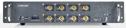
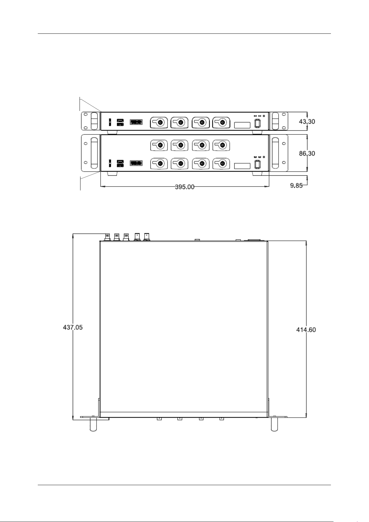
5.1 Mechanical Dimension
Front View
Top View
4-channel model
8-channel model
SDS6000L User Manual
30 i n t . s i g l e n t . c o m
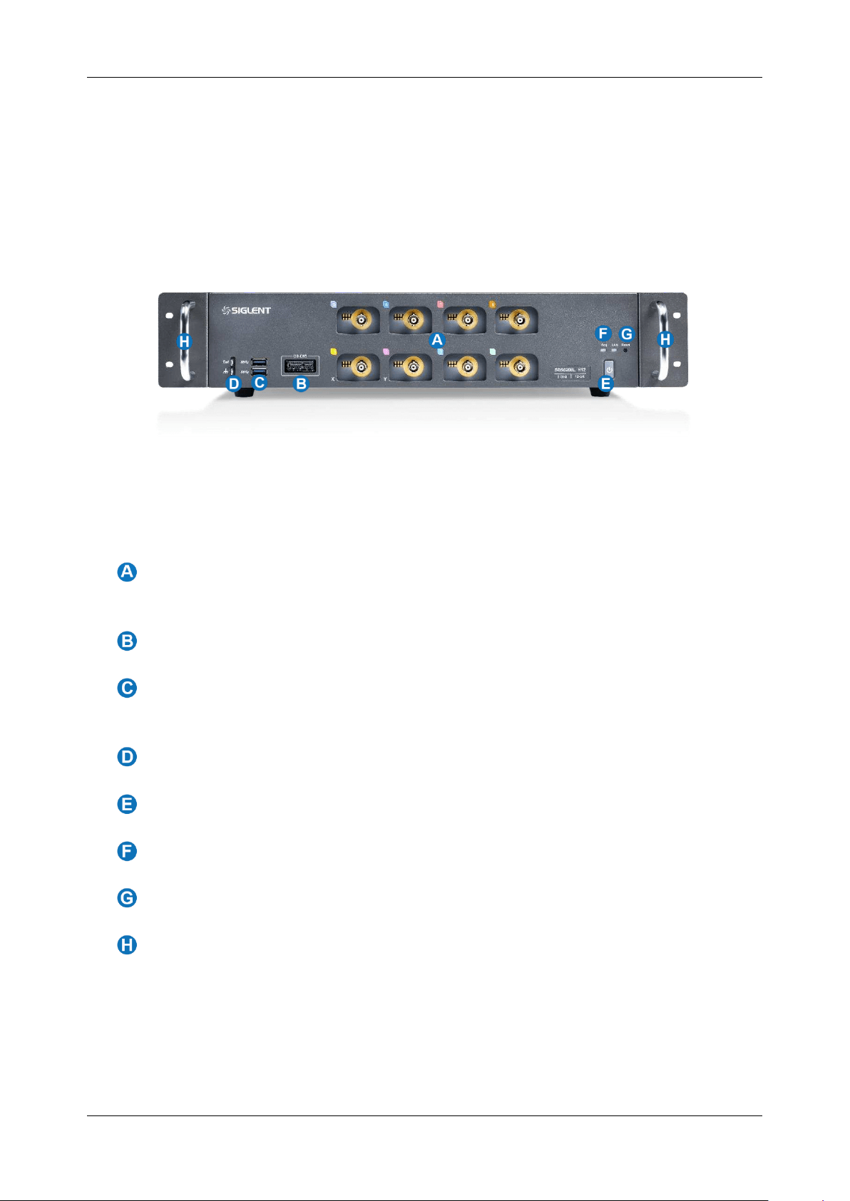
5.2 Front Panel Overview
Analog Input Connectors
1 MΩ: ≤ 400 Vpk (DC + AC), DC~10 kHz; 50 Ω: ≤ 5 Vrms,
±10 V Peak
Digital Input Connector
USB 3.0 Host Ports
Connect to USB storage devices for data transfer or USB
mouse/keyboard for control
Probe Compensation / Ground Terminal
Power Standby Button
Acquisition status and LAN status LEDs
Reset
for LAN
Handles
SDS6000L User Manual
int. s i g l e n t . c o m 31
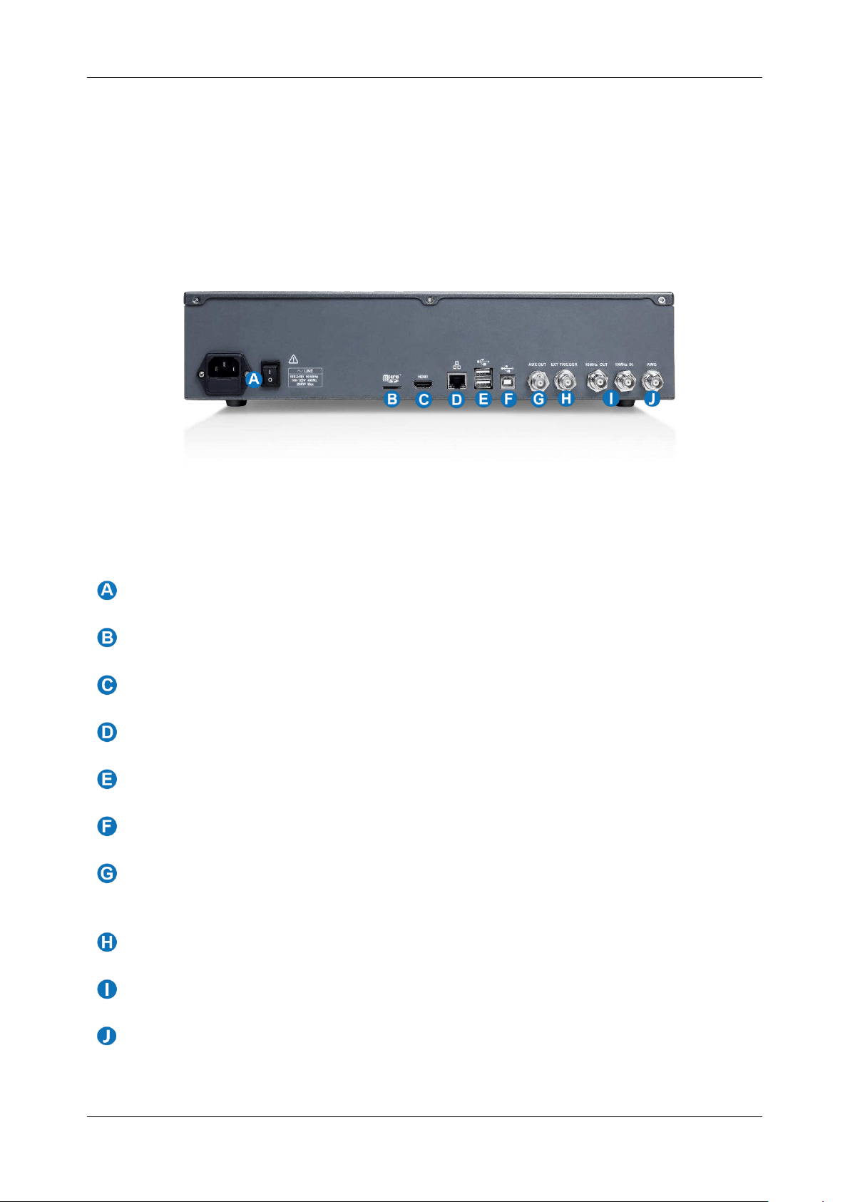
5.3 Rear Panel Overview
AC Power Input and Power Switch
SD Card Slot
HDMI Video Output
Connect the port to an external monitor. The resolution is 1280 * 800
1000M
LAN Port
Connect the port to the network for remote control
USB 2.0 Hosts
Connect with a USB storage device or USB mouse / keyboard
USB 2.0 Device
Connects with a PC for remote control
Auxiliary Out
Outputs the trigger indicator. When Mask Test is enabled, outputs the pass /
fail signal
Ext Trigger Input
10 MHz Out and 10 MHz In
Built-in AWG Output
SDS6000L User Manual
32 i n t . s i g l e n t . c o m
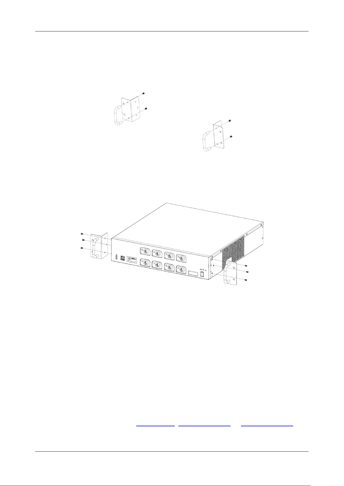
5.4 To Install the Rackmount Flange Kit
1. Install the handles to the left and right rack flange using four M4×8 screws.
2. Install the rack flanges to the instrument using six M3×6 screws.
5.5 Connecting to External Devices/Systems
5.5.1 Power Supply
The standard power supply for the instrument is 100~240 V, 50/60 Hz, or 100~120 V, 400 Hz. Please
use the power cord provided with the instrument to connect it to AC power.
5.5.2 Probes
The SDS6000L series oscilloscope supports active probes and passive probes. The specifications and
probe documents can be obtained at
int.siglent.com, www.siglentna.com, or www.siglenteu.com.
SDS6000L User Manual
int. s i g l e n t . c o m 33
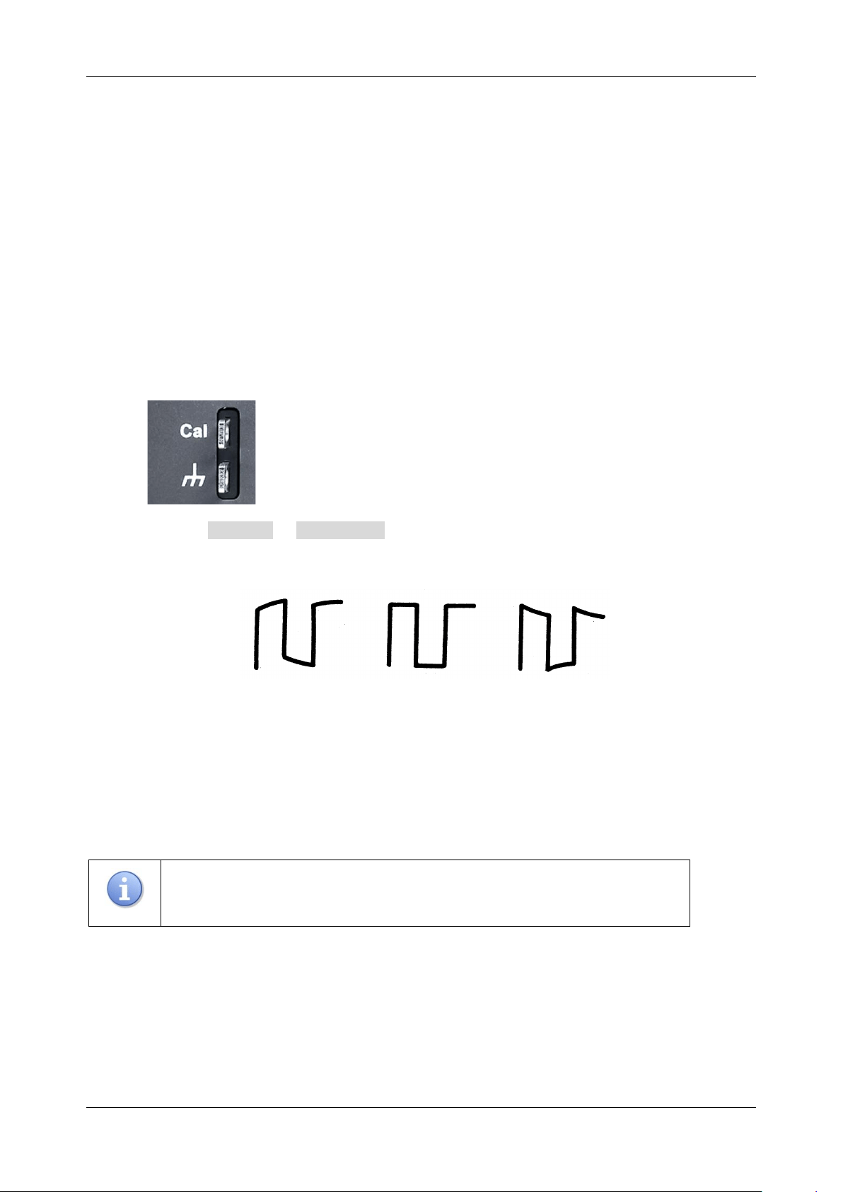
Probe Compensation
When a passive probe is used for the first time, you should compensate it to match the input channel
of the oscilloscope. Non-compensated or poorly compensated probes may increase measurement
inaccuracy or error. The probe compensation procedures are as follows:
1. Connect the coaxial cable interface (BNC connector) of the passive probe to any channel of
the oscilloscope.
2. Connect the probe to the “Compensation Signal Output Terminal” (Cal) on the front of the
oscilloscope. Connect the ground alligator clip of the probe to the “Ground Terminal” under
the compensation signal output terminal.
3. Perform Acquire > Auto Setup .
4. Check the waveform displayed and compare it with the following.
Under
Compensated
Perfectly
Compensated
Over
Compensated
5. Use a non-metallic driver to adjust the low-frequency compensation adjustment hole on the
probe until the waveform displayed is as the “Perfectly compensated” in the figure above.
Note:
It’s not necessary to compensate an active probe.
SDS6000L User Manual
34 i n t . s i g l e n t . c o m
5.5.3 LAN
Connect the LAN port to the network with a network cable with an RJ45 connector for remote control.
See the chapter “ Remote Control ” for detailed information on remotely controlling the instrument.
Follow the steps below to set LAN connection:
Utility > Menu > I/O > LAN Config
See section “LAN” for details of the configuration.
5.5.4 External Monitor and Mouse
Connect an external monitor to the HDMI output on the rear panel of the instrument using an HDMI
cable, and connect a mouse to the instrument, then it can be used as a stand-alone oscilloscope.
5.5.5 Auxiliary Output
When Mast Test is enabled, the port outputs the pass / fail signal, otherwise, it outputs the trigger
indicator. The trigger indicator can be used to measure the waveform capture rate.
See the chapter "Mask Test" for more details on the pass / fail output.

SDS6000L User Manual
int. s i g l e n t . c o m 35
5.5.6 Reference Input and Output
The device can use the internal 10 MHz clock or a 10 MHz clock from another instrument or source
using the 10 MHz In port as the reference. The reference clock is a 10 MHz square wave and can be
output from the 10 MHz Out port for synchronizing other instruments. To set the reference clock by
following the steps:
Utility > Menu > IO > Clock Source
See the "Clock Source" section for details.
5.5.7 Waveform Generator
Activate the SDS6000L-FG option to support the waveform generator function.
Perform Utility > AWG Menu to set the waveform.
See chapters “Waveform Generator” and “Bode Plot” for more relative information.
5.5.8 Logic Probe
To connect the logic probe:
Insert the probe, with the correct side facing up, until you hear a
“click”.
To remove the logic probe:
Depress the buttons on each side of the probe, then pull out it.
See the chapter “Digital Channels” for more information.
SDS6000L User Manual
36 i n t . s i g l e n t . c o m
5.6 Power on
The SDS6000L provides two ways to power on, which are:
Auto Power-on
When the “Auto Power-on” option is enabled, once the oscilloscope is connected to the AC power
supply through the power cord, the oscilloscope boots automatically. This is useful in automated or
remote applications where physical access to the instrument is difficult or impossible.
Steps for enabling the "Auto Power-on" function:
Utility > Menu > System Setting > Auto Power On
Power on by Manual
When the " Auto Power on” option is disabled, the power button on the front panel is the only control
for the power state of the oscilloscope.
5.7 Shut down
Press the power button for one second to turn off the oscilloscope. Or follow the steps below:
Utility > Shutdown
Note:
The front panel Power button does not disconnect the oscilloscope from
the AC power supply. To disconnect the instrument from the mains, turn off
the power switch on the rear panel of the instrument. The power cord should
be unplugged from the AC outlet if the scope is not to be used for an
extended period. The standby power consumption of the 4-channel model is
about 4 W, and that of the 8-channel model is about 8 W.

SDS6000L User Manual
int. s i g l e n t . c o m 37
5.8 System Information
Follow the steps below to examine the software and hardware versions of the oscilloscope.
Utility > Menu > System Info
See the section "System Information" for details.
5.9 Install Options
A license is necessary to unlock a software option. See the section "Install Option" for details.
SDS6000L User Manual
38 i n t . s i g l e n t . c o m
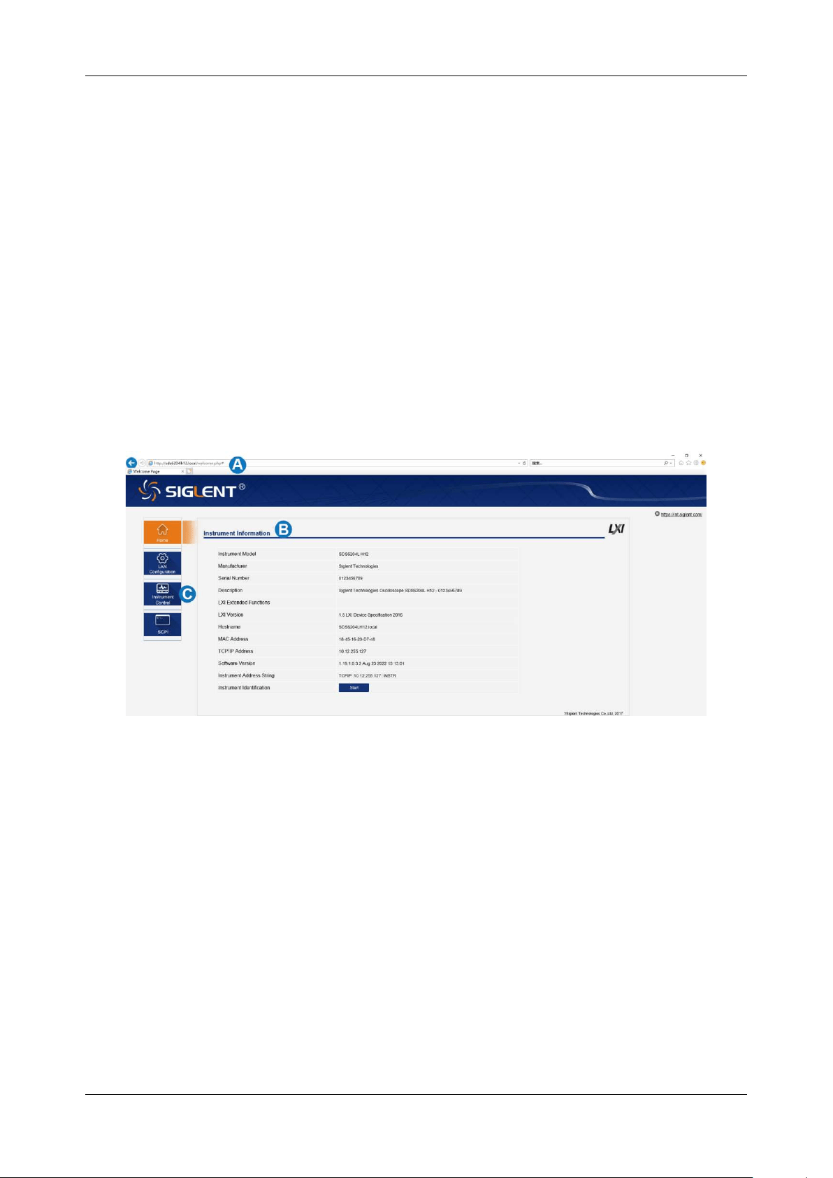
6 Remote Control
The SDS6000L provides a LAN port and a USB Device port which can be used for remote control in
multiple ways.
6.1 Web Browser
A built-in web server provides an approach to interact with the oscilloscope by a web browser. It doesn’t
require any additional software to be installed on the computer. Set the LAN port correctly (see section
“LAN” for details), input the IP address of the oscilloscope in the browser address bar, and then the
user can browse and control the oscilloscope on the web.
A. Input the IP address of the instrument
B. Instrument information
C. Click here to recall the instrument control interface

SDS6000L User Manual
int. s i g l e n t . c o m 39
Below is the instrument control interface:
A. The display and control area of the instrument’s web control interface. The display in this
area is a copy of the instrument display. Using the mouse to operate in this area is equivalent
to directly operating the touch screen display of the instrument.
B. Click here to perform a screenshot
C. Click here to save the waveform data as a bin file and download it to the local computer
D. Click here to save the waveform data as a CSV file and download it to the local computer
E. Click here to download the mini-tool for converting binary files to CSV
F. Click here to perform a firmware upgrade
6.2 Other Connectivity
The SDS6000L also supports remote control of the instrument by sending SCPI commands via NI-
VISA, Telnet, or Socket. For more information, refer to the programming guide for this product.
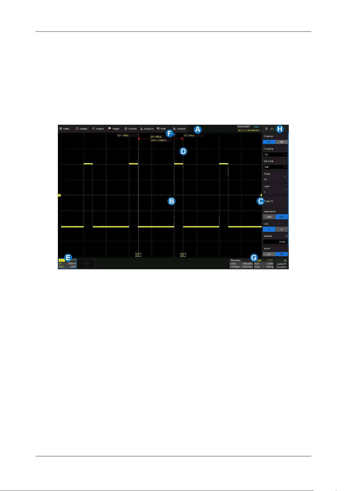
SDS6000L User Manual
40 i n t . s i g l e n t . c o m
7 Screen Display
7.1 Overview
When an external monitor is connected or a web server is used, the entire screen can be manipulated
using a mouse.
A. Menu Bar
B. Grid Area
C. Trigger Level Indicator
D. Cursors
E. Channel Descriptor Boxes
F. Trigger Delay Indicator
G. Timebase and Trigger Descriptor Boxes
H. Dialog Box

SDS6000L User Manual
int. s i g l e n t . c o m 41
Trigger Level Line
(Vertical) and
Trigger Delay Indicator
(Horizontal) show the trigger position of the
waveform.
Cursors
show where measurement points have been set. Move the cursors to quickly reposition the
measurement point.
Channel Descriptor boxes
include analog channels (Cx), zoom traces (Zx), digital channels (D), math
(Fx), memory (Mx), and reference (Ref). They are located under the grid area, showing the parameters
of the corresponding traces. Clicking the boxes creates a dialog box.
Timebase and Trigger Descriptor boxes
show the parameters of the timebase and trigger
respectively. Clicking the boxes creates a dialog box for the selected item.
7.2 Menu Bar
Menu bar with drop-down menus lets you access set-up dialogs and other functions.
7.3 Grid Area
The grid area displays the waveform traces. Traces can be moved by the mouse. The area is divided
into 8 (vertical) * 10 (horizontal) grids. The best display effect can be obtained by adjusting the
waveform intensity and graticule. Follow the steps below to set these parameters:
Display > Menu > Intensity ,
Display > Menu > Graticule
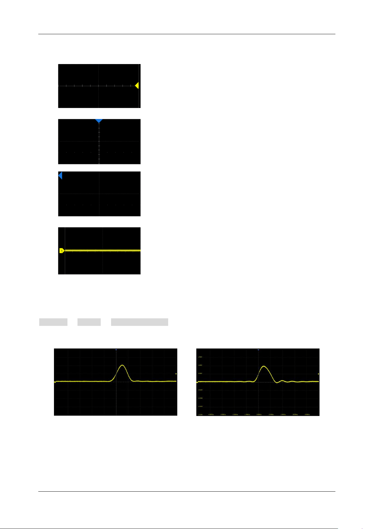
SDS6000L User Manual
42 i n t . s i g l e n t . c o m
There are multiple indicators on the grid:
Trigger Level Indicator
shows
the level where the waveform
triggers on the vertical axis.
Trigger Delay Indicator
locates
where the waveform triggers on
the horizontal axis... When the
trigger position is outside the
screen, the direction of the
triangle changes to point outside
the screen.
Channel Offset Indicator
with a
channel number shows the offset
position of the corresponding
channel.
The user can choose to show the axis labels or not by:
Display > Menu > Axis label Setting
Axis label = on
Axis label = off
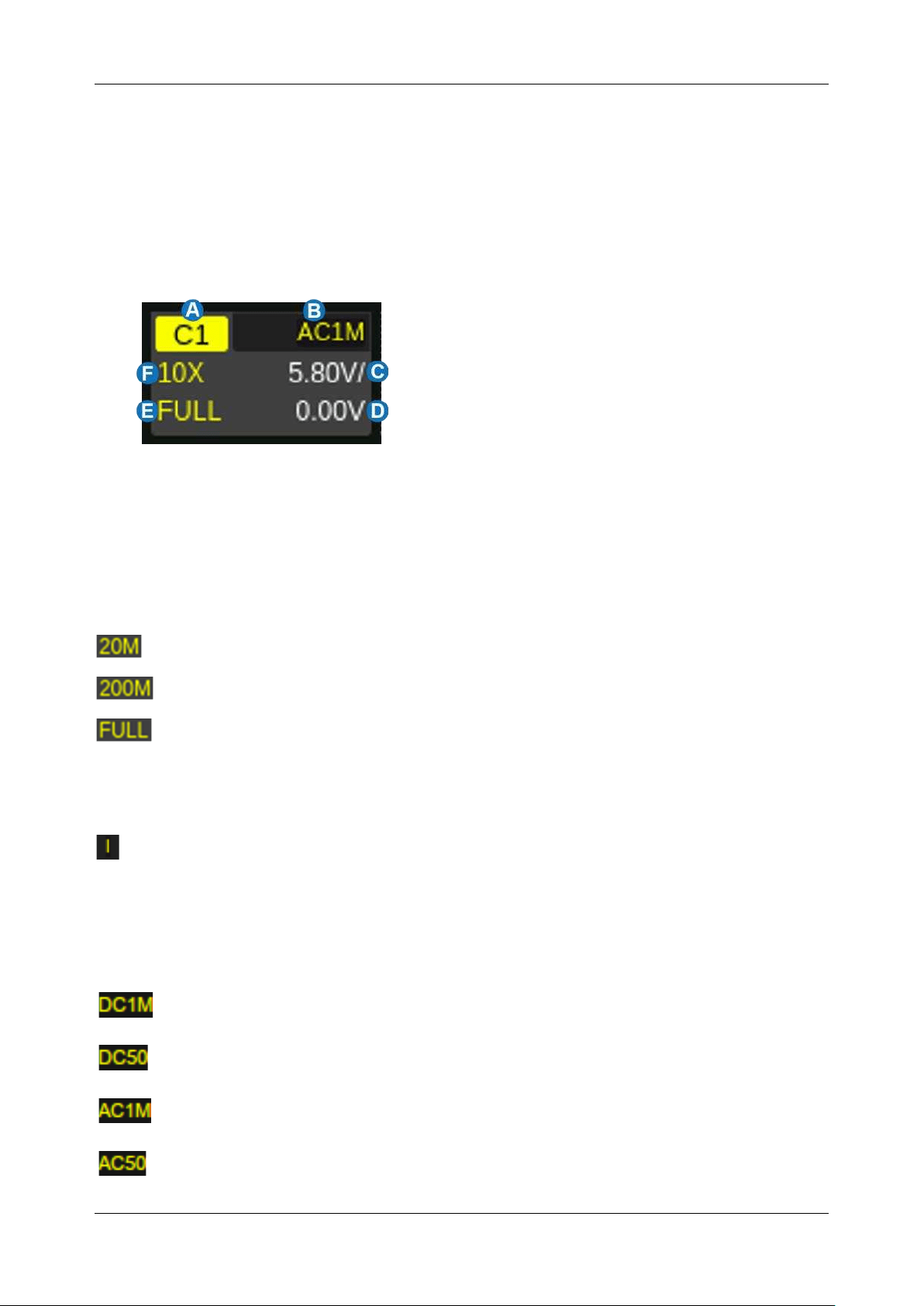
SDS6000L User Manual
int. s i g l e n t . c o m 43
7.4 Channel Descriptor Box
Channel Descriptor boxes include analog channels (Cx), zoom traces (Zx), digital channels (D), math
(Fx), memory (Mx), and reference (Ref). They are located under the grid area, showing the parameters
of the corresponding traces. Clicking the boxes creates a dialog box. See the chapter “Vertical Setup”
for more details. Below is an example for analog channel 1:
A. Channel Index
B. Coupling and Input Impedance
C. Vertical Scale
D. Vertical Offset
E. Bandwidth Information
F. Probe Attenuation Factor
Bandwidth Information:
The bandwidth information is indicated by the following icons:
: 20 MHz bandwidth limit
: 200 MHz bandwidth limit
: Full bandwidth
Invert Indicator
: shows that the current channel is inverted:
: Invert has been turned on
None:
Invert has been turned off
Coupling and Input Impedance:
:
DC coupling, 1 MΩ impedance
:
DC coupling, 50 Ω impedance
:
AC coupling, 1 MΩ impedance
:
AC coupling, 50 Ω impedance
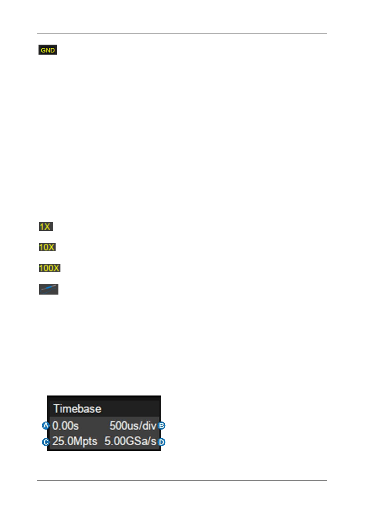
SDS6000L User Manual
44 i n t . s i g l e n t . c o m
:
Ground
Vertical Scale:
The scale of each grid in the vertical direction. For example, when the vertical scale is
1.00 V/div, the full scale of the oscilloscope is 1.00 V/div * 8 div=8 V.
Vertical Offset:
The offset of the channel in the vertical direction. When the vertical offset is 0, the
channel offset indicator is located in the middle of the vertical axis.
Probe Attenuation Factor:
Set the probe attenuation factor to match the actual attenuation of the
probe. The oscilloscope automatically calculates the vertical scale according to the probe attenuation
factor. For example, the vertical scale of the oscilloscope is 100mV/div with 1X attenuation, and 1 V/div
if the attenuation factor is changed to 10X. When inserting a standard 10X passive probe with a probe
sense terminal, the oscilloscope will automatically set the factor to 10X.
:
1:1 attenuation, suitable for direct coaxial cable connection or passive probes with 1X attenuation
:
10:1 attenuation, suitable for general passive probes or active probes with 10X attenuation
:
100:1 attenuation, suitable for some high-voltage probes
:
Custom attenuation factor
7.5 Timebase and Trigger Descriptor Boxes
The Timebase Descriptor box
shows the current parameters of the timebase. See the chapter
“Horizontal and Acquisition Setup” for more information.
A. Trigger delay
B. Horizontal scale
(
timebase
)
C. # Samples
D. Sample Rate
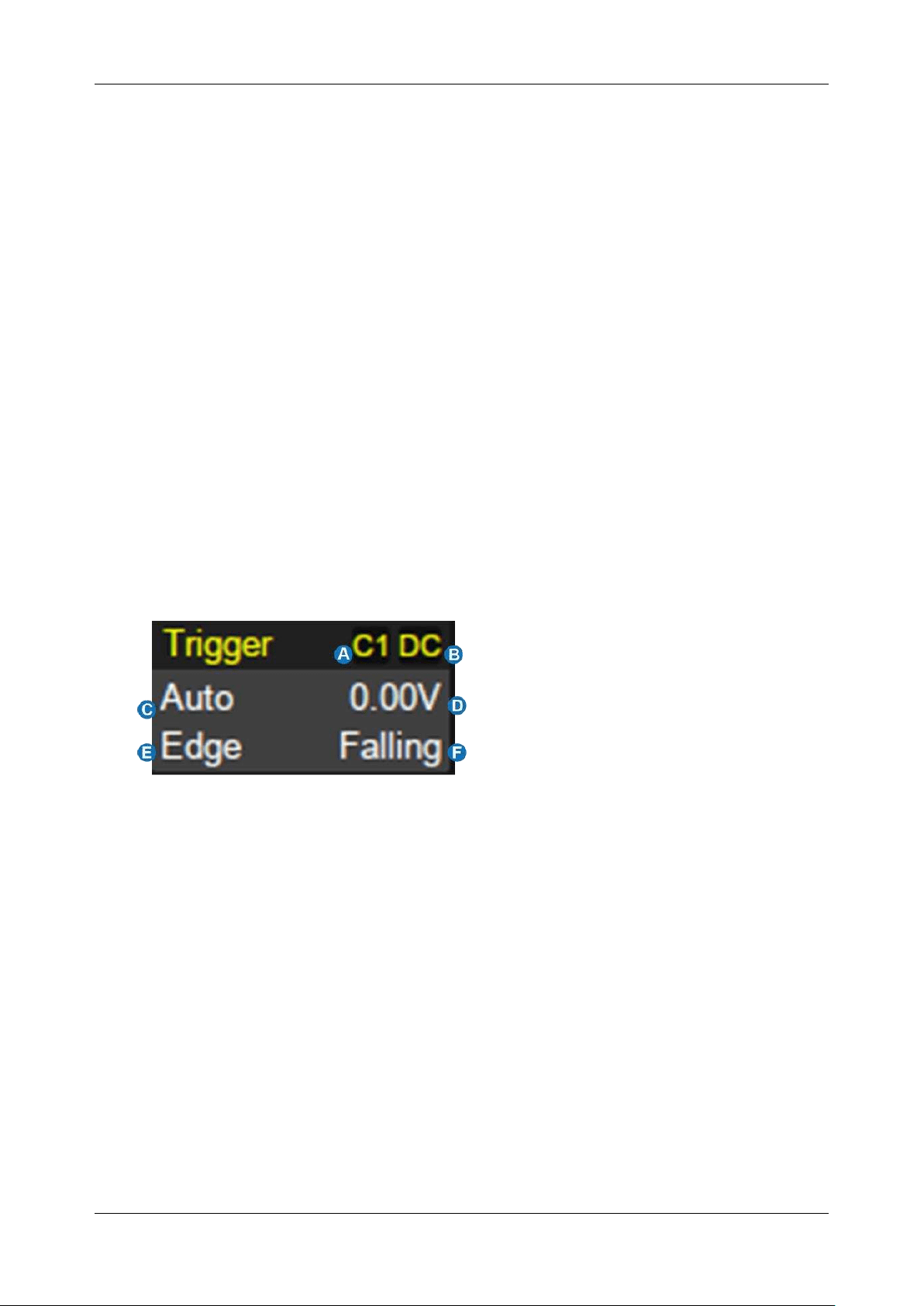
SDS6000L User Manual
int. s i g l e n t . c o m 45
Trigger delay:
The time offset of trigger position. When the trigger delay is 0, the trigger delay indicator
is in the center of the horizontal axis of the grid area.
Horizontal scale:
Timebase, the time of each grid in the horizontal direction. For example, if the scale
is 500us/div, the time of each grid is 500 us, and the full-screen time range of the oscilloscope is 500
us/div * 10 div = 5 ms.
# Samples:
The number of sample points on the current screen.
Sample Rate:
The current sample rate.
The Trigger Descriptor box shows the parameters of the trigger setting. See the chapter “Trigger” for
detailed information.
A. Trigger source
B. Trigger coupling
C. Trigger mode
D. Trigger level
E. Trigger type
F. Trigger slope
Trigger source
C1~C8: Analog channels
EXT: External trigger channel
EXT/5: 5x attenuation of external trigger channel
AC Line: AC mains supply
D0~D15: Digital channels

SDS6000L User Manual
46 i n t . s i g l e n t . c o m
Trigger coupling:
Coupling mode of the current trigger source. It is only valid when the trigger source
is C1~C8, EXT, or EXT/5.
DC: All the signal’s frequency components are coupled to the trigger circuit for high-frequency
bursts or where the use of AC coupling would shift the effective trigger level.
AC: The signal is capacitively coupled. DC levels are rejected. See the datasheet for details of the
cut-off frequency.
HFR: Signals are DC coupled to the trigger circuit, and a low-pass filter network attenuates high
frequencies (used for triggering on low frequencies). See the datasheet for details of the cut-off
frequency.
LFR: The signal is coupled through a capacitive high-pass filter network, DC is rejected and low
frequencies are attenuated. For stable triggering on medium to high-frequency signals. See the
datasheet for details of the cut-off frequency.
Trigger mode
Auto: The oscilloscope will sweep without a set trigger. An internal timer triggers the sweep after
a preset timeout period so that the display refreshes continuously. This is helpful when first
analyzing unknown signals. Otherwise, Auto functions the same as Normal when a trigger
condition is found.
Normal: Sweeps only if the input signal meets the trigger condition. Otherwise, it continues to
display the last acquired waveform.
Single: Stops the acquisition and displays the last acquired waveform.
Force: Force an acquisition, regardless of whether the input signal meets the trigger conditions or
not.
Trigger level
: The source voltage level or levels that mark the threshold for the trigger to fire. Trigger
levels specified in Volts normally remain unchanged when the vertical gain or offset is modified.
Trigger type:
See the chapter "Trigger" for details.
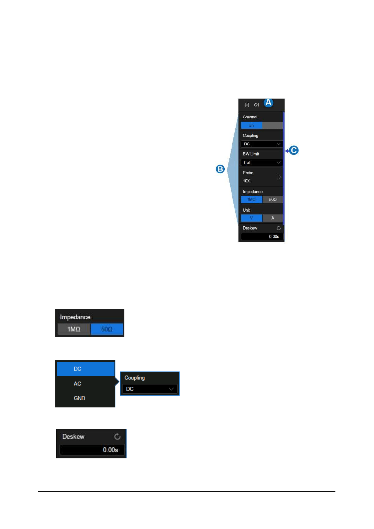
SDS6000L User Manual
int. s i g l e n t . c o m 47
7.6 Dialog Box
The dialog box on the right side of the screen is the main area for setting the parameters of the selected
function.
A. Title bar. Clicking the bar can hide the
dialog box, and clicking again can open
the dialog box.
B. Parameter setting area.
C. Scroll bar. When parameters are more
than the displayed range, the blue
scrollbar will be displayed. By sliding the
dialog area up and down, it can scroll to
the area not displayed.
To Set Parameters
The SDS6000L provides a couple of different ways to input/select parameters:
Switch:
Sets parameters with two states, such as to enable or
disable a function. Click the switch region to change from one
state to the other.
List:
Sets parameters with more than two
options, such as coupling mode of
channels. Click the parameter region, and
then select the expected option from the
pop-up list.
Virtual Keypad:
Sets parameters with a numerical value. Click
the parameter region, and the parameter can be adjusted by
the mouse wheel; click the region again, then the virtual keypad
appears:
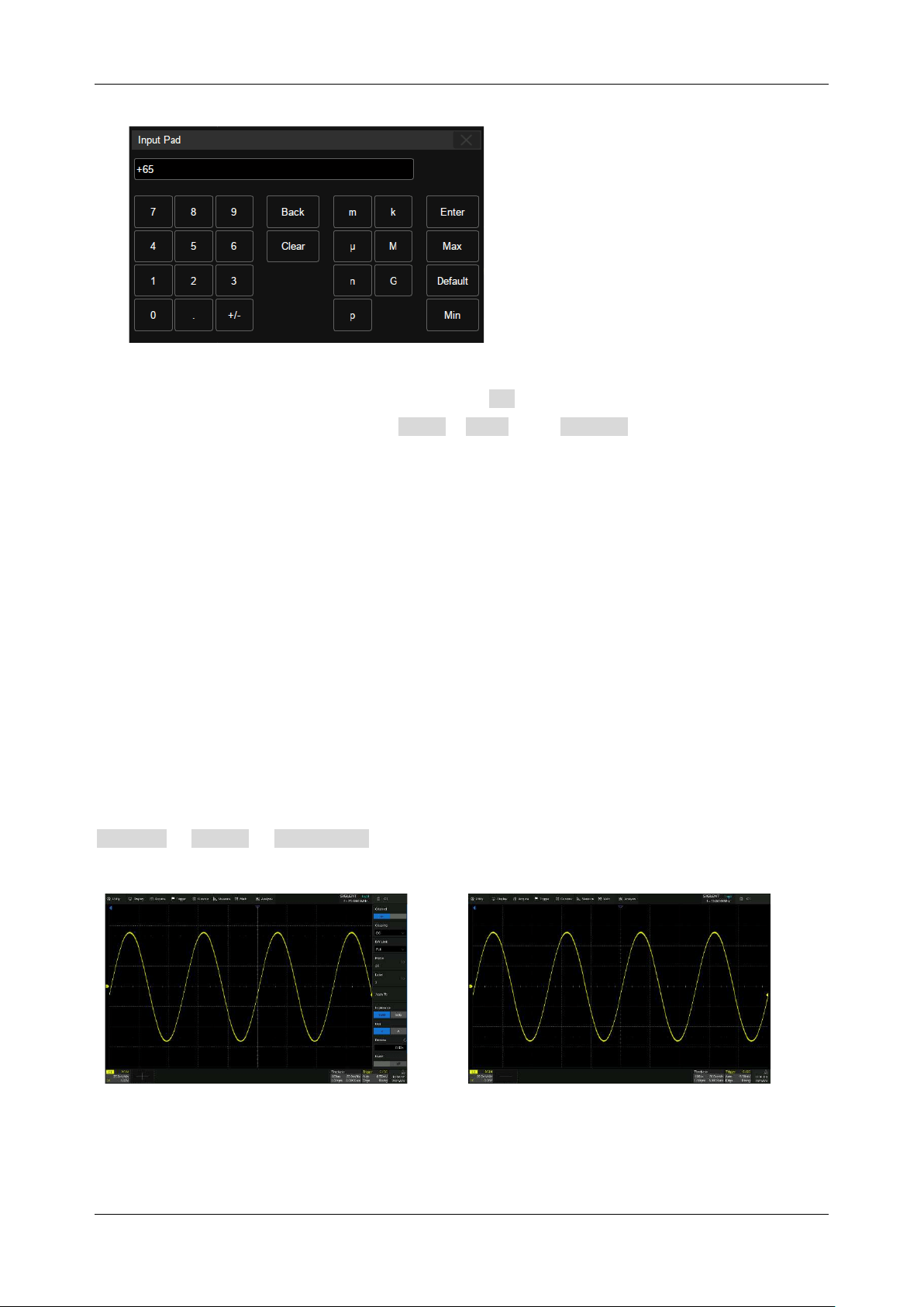
SDS6000L User Manual
48 i n t . s i g l e n t . c o m
Let’s use the operation of setting the “deskew” of a channel as an example: If the expected value is 65
ns, input “65” on the virtual keypad, and then choose n as the unit “ns” to complete the operation.
On the virtual keypad, clicking the button Max , Min , and Default quickly sets the parameter
to the maximum, minimum, and default values.
Hide Dialog Box
When the menu style is set to “Embedded”, the grid area will be compressed horizontally to display the
complete waveform when the dialog box is displayed. After setting the parameters, to achieve the best
waveform display effect, click the title bar in the upper right corner to hide the dialog box. Click it again
to recall the dialog box.
When the menu style is set to “Floating”, it will directly cover part of the grid area when displayed. If
you want to observe the covered area, click the title bar in the upper right corner to hide the dialog box.
Click it again to recall the dialog box.
The dialog box can be set to be hidden automatically. When the instrument is not operated beyond the
set time, the dialog box will be automatically hidden. Follow the steps below:
Display > Menu > Hide Menu .
Menu style = Floating, and the Dialog box is
displayed
Dialog box is hidden
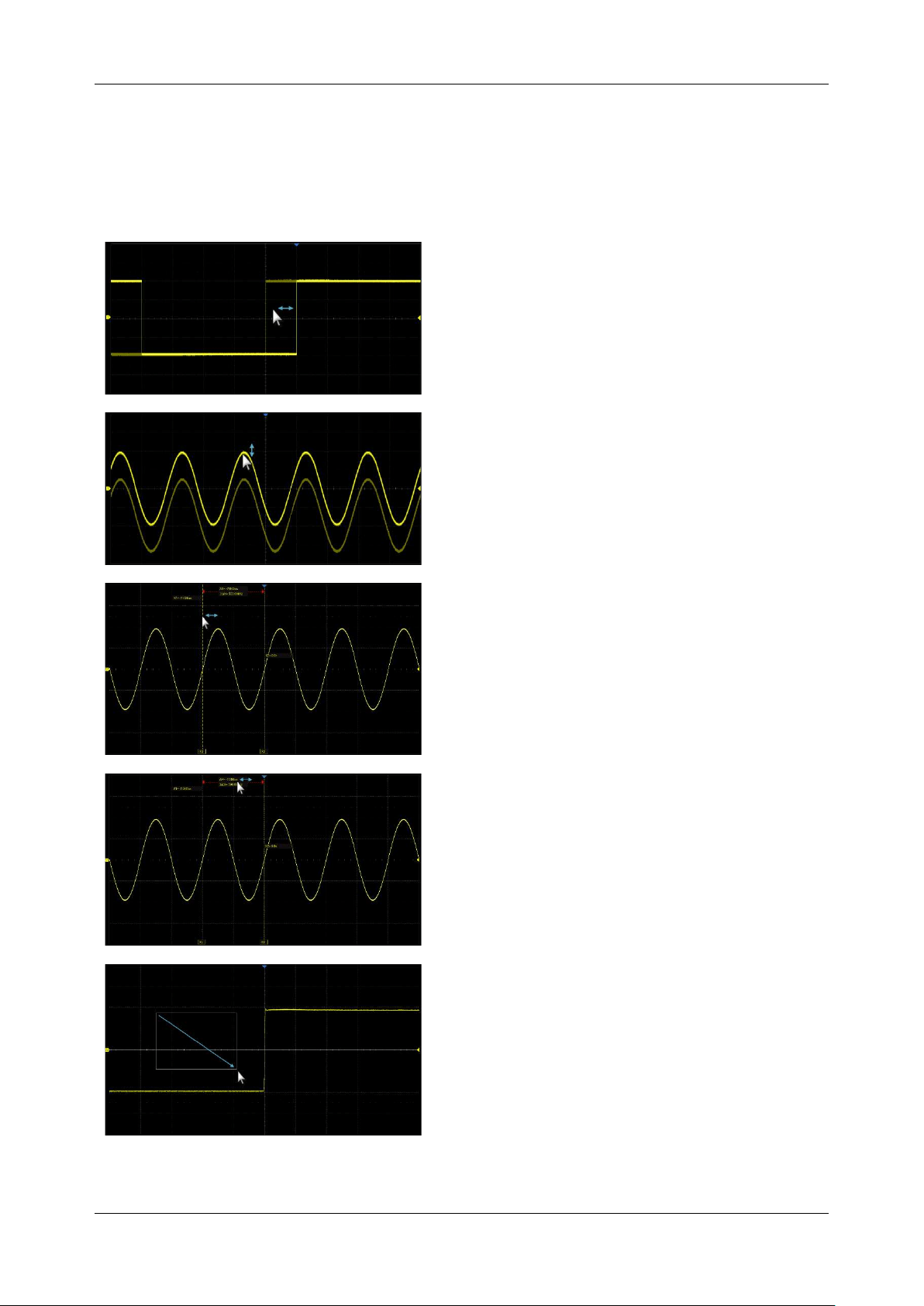
SDS6000L User Manual
int. s i g l e n t . c o m 49
7.7 Mouse Control
Waveforms, cursors, and trigger levels can be adjusted using the mouse. It can also be used to define
Zone Trigger areas as shown below:
Click-and-drag the waveform left and right to
move it on the horizontal axis
Click-and-drag the waveform up and down to
move it on the vertical axis
Click-and-drag the cursor to move it
Click-and-drag the cursor information region
to move the pair of cursors simultaneously
Click-and-drag along a diagonal line to
create a zone or a histogram region. At the
beginning of the drawing action keep the
angle close to 45° so it can be recognized as
the drawing box action

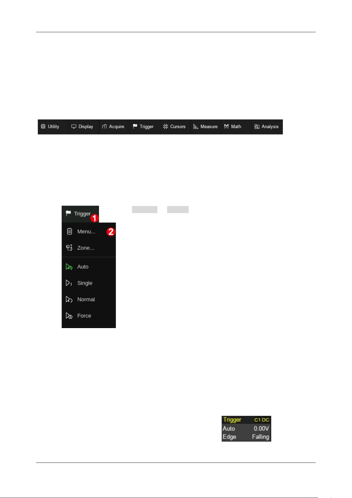
SDS6000L User Manual
int. s i g l e n t . c o m 51
8 Multiple Approaches to Recall Functions
The oscilloscope can recall functions through different approaches.
8.1 Menu Bar
If you are familiar with common computer programs, you may first choose to access a function by the
drop-down menu from the menu bar at the top of the display.
For example, to open the trigger setup dialog box, you can follow the steps below:
Trigger > Menu
The operations can be completed with mouse clicks.
8.2 Descriptor Box
For the setup of channels, zoom traces, math, ref, memory traces, timebase, and trigger, there are
dialog boxes at the bottom of the display. For the introduction of the descriptor box, see sections
"Channel Descriptor Box" and "Timebase and Trigger Descriptor Box".
For the example above, click the trigger descriptor box and the
trigger setup dialog box will be activated.
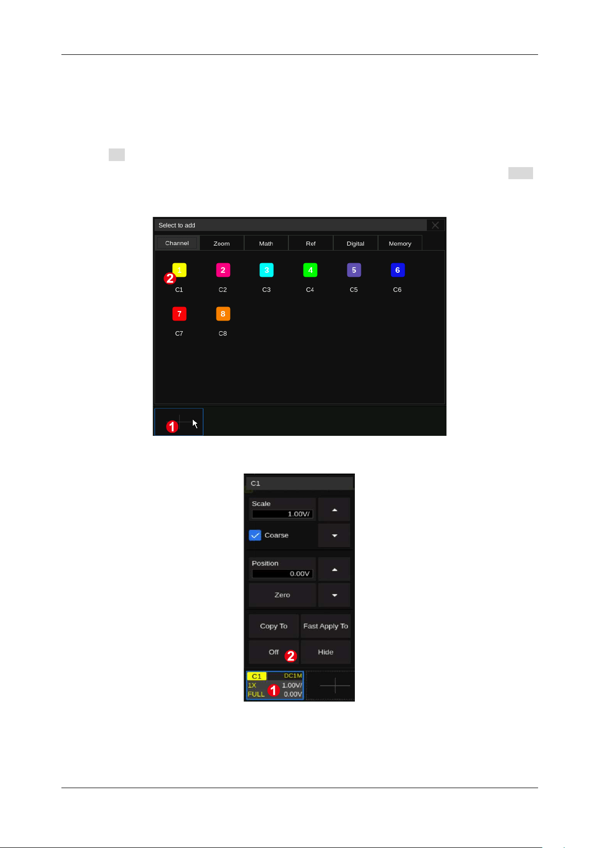
SDS6000L User Manual
52 i n t . s i g l e n t . c o m
9 Vertical Setup
9.1 Turn on/off a Channel
Click the + button and then select the expected channel to turn it on, and its channel descriptor box
and a dialog box will appear on the display. Click the channel descriptor box and then click the Off
button to disable it.
Turn on C1
Turn off C1
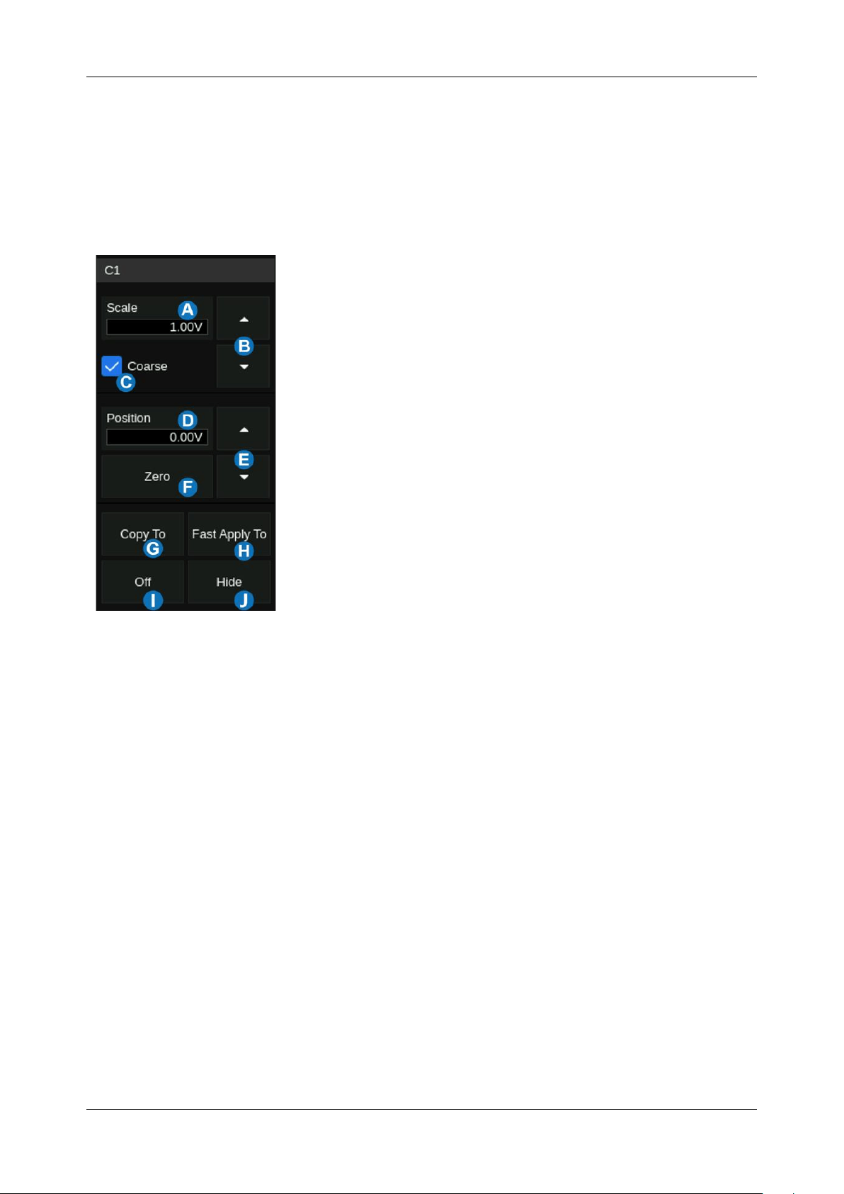
SDS6000L User Manual
int. s i g l e n t . c o m 53
9.2 Channel Setup
Click the channel descriptor box, a quick dialog will pop up. Vertical scale and offset can also be set
from this dialog box.
A. Click the region to set the vertical scale with the
mouse wheel or virtual keypad
B. ▲ to increase the vertical scale and ▼ to
decrease
C. Check to coarsely adjust the vertical scale and
uncheck to enable fine adjustment
D. Click the region to set the offset with the mouse
wheel or virtual keypad
E. ▲ to increase the offset and ▼ to decrease
F. Set the offset to zero
G. Copy the setting of the current channel to another
channel
H. Quickly apply the current channel as the source of
a specified operation (Trigger, FFT, Simple
Measure, Cursor, Search, DVM, and Counter)
I. Disable the channel
J. Hide the trace
The vertical scale can be adjusted in coarse or fine mode. Fine mode can reach the full-scale display
as close as possible, which gets the best measurement accuracy in the vertical direction.
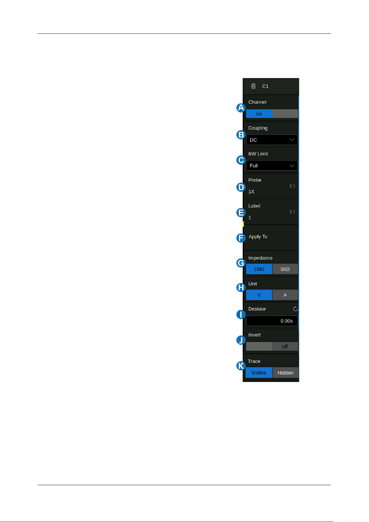
SDS6000L User Manual
54 i n t . s i g l e n t . c o m
Activating a channel recalls the channel dialog box, displaying more parameters:
A. Turn the channel on/off
B. Coupling (DC, AC, or GND)
C. Bandwidth limit (Full, 200 MHz, or 20 MHz)
D. Probe settings including attenuation (1X, 10X,
100X, or custom) and probe check. If an active
probe is connected, it shows the information and
setup of the active probe
E. Set the label text. Click to recall the label setting.
Users can customize the text and display of the
label
F. Quickly apply a specified operation (Trigger, FFT,
Simple Measure, Cursor, Search, DVM,
Histogram, Mask Test, Counter, and AWG) to the
current channel
G. Impedance
H. Units for the channel
I. Deskew
J. Enable/disable invert
K. Trace visible/hidden
Coupling
DC: All of the input signal frequency components are passed to the display.
AC: The signal is capacitively coupled. DC signal components are rejected. See the datasheet for
details of the cut-off frequency.AC coupling is suitable for observing AC signals with DC offset,
such as power ripple.

SDS6000L User Manual
int. s i g l e n t . c o m 55
GND: The channel is grounded by an internal switch. GND coupling is used to observe the zero-
offset error of the analog channels or determine the source of noise in the waveform (from the
signal or from the oscilloscope itself)
Bandwidth Limit
Full bandwidth passes through signals with high-frequency components, but it also means that noise
with high-frequency components can pass through. When the frequency component of the signal is
very low, better signal-to-noise ratios (SNR) can be obtained by turning on a bandwidth limit. The
SDS6000L provides two hardware bandwidth limit options: 20 MHz and 200 MHz
Probe Settings
The SDS6000L provides 1X, 10X, 100X, and custom probe attenuation factor options. The custom
values can be between 10
-6
~10
6
. The oscilloscope will automatically convert the vertical scale
according to the current probe attenuation factor. For example, the vertical scale of the oscilloscope
under 1X attenuation is 100 mV/div, and the vertical scale will be automatically set to 1 V/div if the
probe attenuation is changed to 10X. If a standard probe with a readout terminal is connected, the
oscilloscope will automatically set the probe attenuation to match the probe.
The Probe Check option is provided to quickly check if the probe is correctly compensated. Connect
the probe as in section “Probes” and click Probe > Probe Check , then operate according to the
prompt.
If an active probe is connected, click Probe to show the information and setup of the active probe.
Below is the information for an SAP1000 probe.
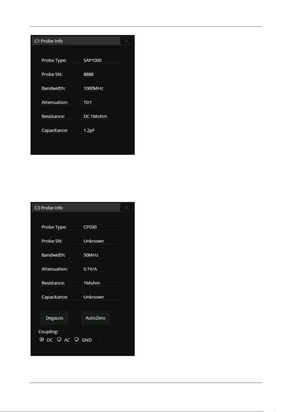
SDS6000L User Manual
56 i n t . s i g l e n t . c o m
For some active probes that need to be controlled from the UI, the Probe dialog provides the necessary
setup. Below is an example of a current probe, of which the Degauss, Autozero, and Coupling options
are accessible.
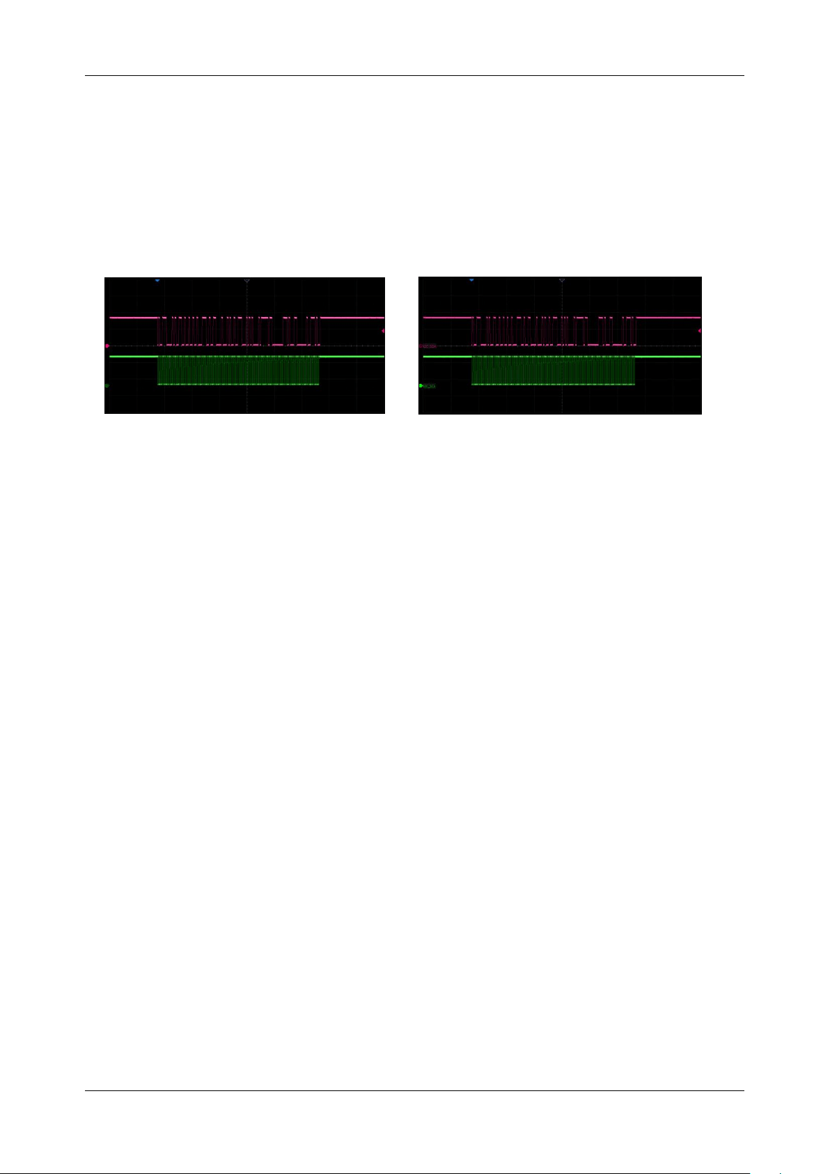
SDS6000L User Manual
int. s i g l e n t . c o m 57
Label
Users can set the label text for channels. Open the label setting dialog box to select the source,
customize the label text, and set the display. The source can be C1~C8, F1~F4, M1~M4, and
RefA~RefH. The length of the label is limited to 20 characters. The characters beyond this length will
not be displayed. When the “Display” option is set to “on”, the label will be displayed on the right side
of the channel offset indicator.
The labels are hidden
The labels are displayed
Apply to
With this setting, some common functions such as Trigger, FFT, Simple Measure, Cursor, Search,
DVM, Histogram, Mask Test, Counter, and AWG can be quickly applied to the selected channel. Once
a function is specified, it will switch directly to the function menu and automatically set that channel as
the source.
Impedance
1 MΩ: When a passive probe with high impedance is connected, the impedance must be set to 1
MΩ, otherwise the signal will not be detected.
50 Ω: Suitable for high-frequency signals transmitted through 50 Ω coaxial cables or active probes.
This can minimize the amplitude distortion caused by impedance mismatching.
Unit
Voltage unit "V" or current unit "A”. When using the current probe, the unit should be set to "A".
Deskew
Due to the skew between channels, cables, or probes, the delay of signals passing through different
measurement paths may be inconsistent. For example, two coaxial cables with a 1-inch difference in
length could introduce a skew of more than 100 ps. In some scenarios (e.g. measuring the setup/hold
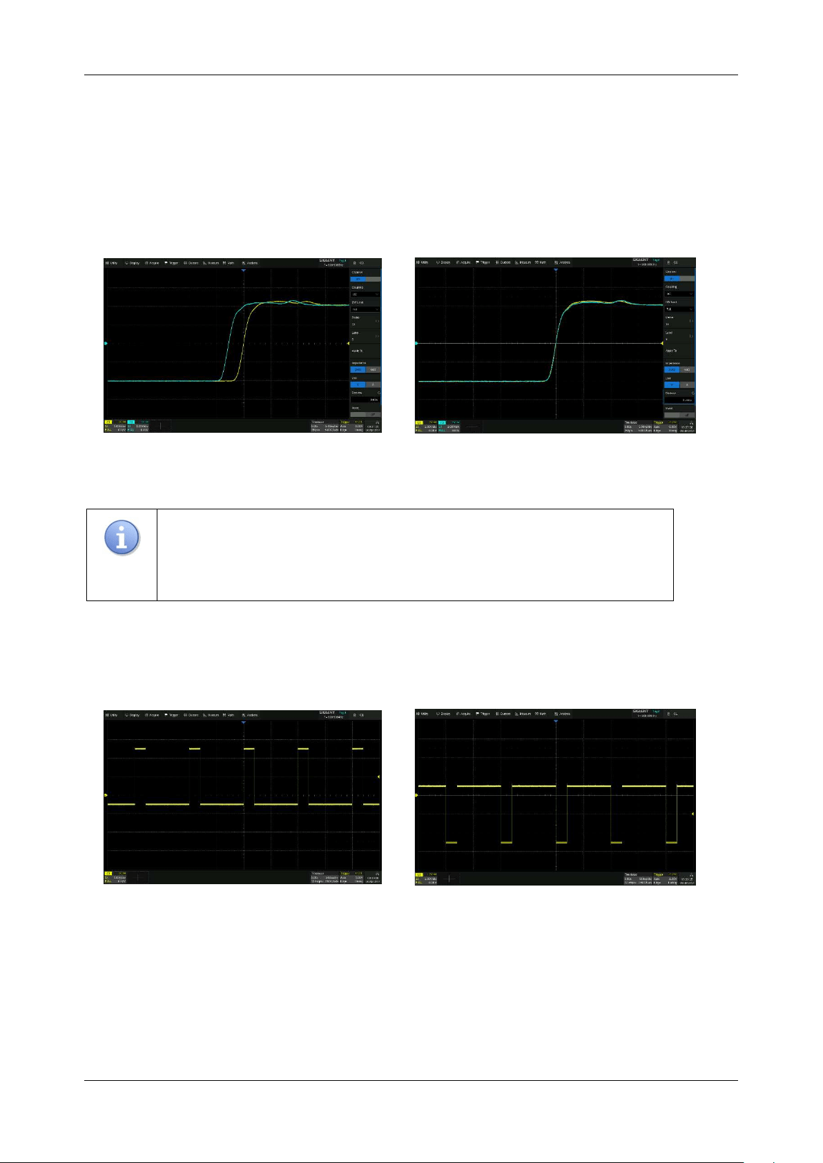
SDS6000L User Manual
58 i n t . s i g l e n t . c o m
time between the clock and data), it may be necessary to compensate for the skew between channels.
The method of compensation: Probe the same signal simultaneously using two channels (including the
cables or probes that you intend to use for measurements) and adjust the deskew parameter of one
channel until the waveforms of the two channels observed on the screen coincide horizontally.
Before deskew
After deskew
Note:
When the channel with delay compensation is the trigger source, the
trigger delay indicator will not change at any time when the deskew value
changes.
Invert
When invert is enabled, the waveform is rotated 180 degrees around earth potential (0 Volts).
Before invert
After invert
SDS6000L User Manual
int. s i g l e n t . c o m 59
Trace
When the trace is hidden, the channel waveform is no longer displayed on the screen, while the
acquisition is still running in the background.
Trace visible
Trace hidden
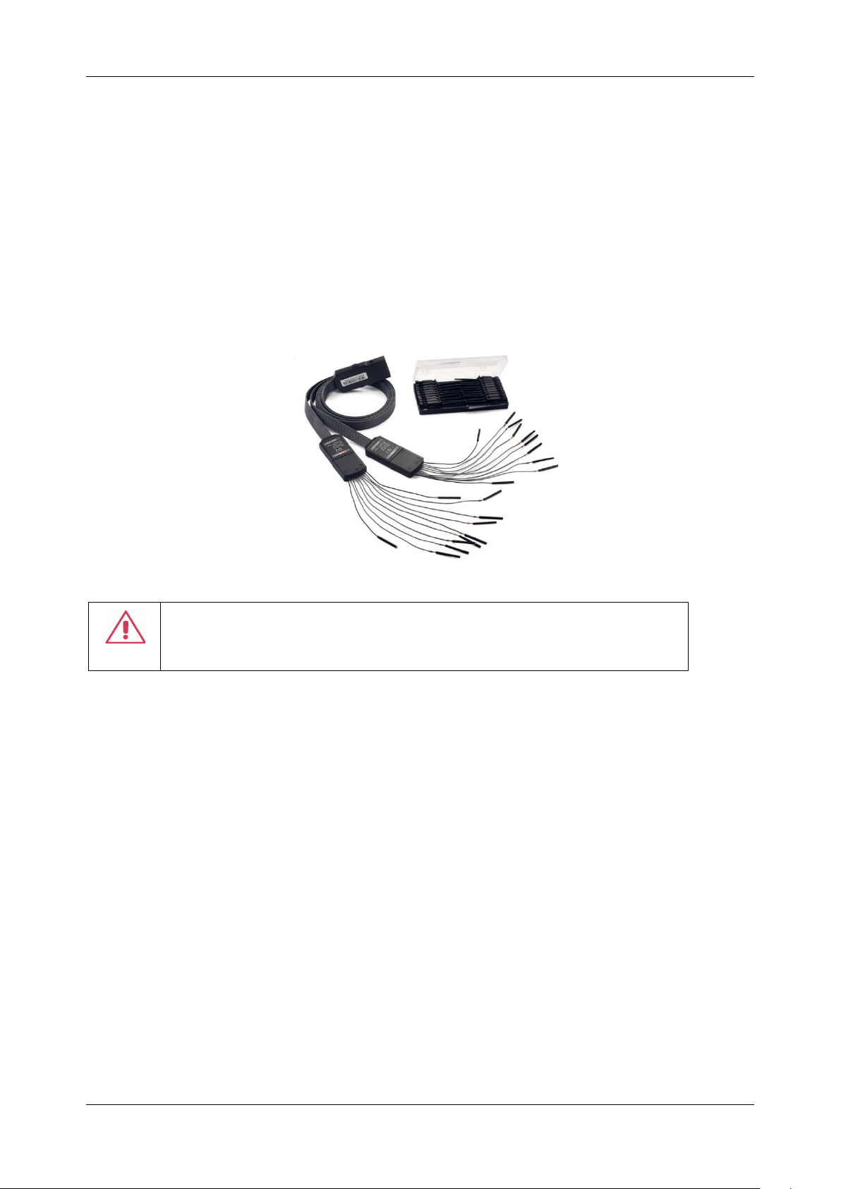
SDS6000L User Manual
60 i n t . s i g l e n t . c o m
10 Digital Channels
10.1 Overview
SPL2016 Probe
The SPL2016 is a logic probe designed to monitor up to 16 digital signals at once. The 16 digital
channels are separated into two groups and each group has its threshold, making it possible to
simultaneously view data from different logic families.
To avoid personal injury or damage to the logic probe and any associated
equipment, the following safety precautions should be noted.
The equipment shall be used only for the purposes specified by the manufacturer.
The SPL2016
probe is used only for SIGLENT's special series of oscilloscopes. Protection mechanisms can be
compromised if the way the devices connected by the SPL2016 are not used for their intended purpose.
Connect and disconnect correctly.
Excessive bending can damage the cable.
Do not use equipment in humid or explosive environments.
Only used indoors.
The SPL2016 is designed to be used indoors and should only be operated in a
clean, dry environment.
Do not use the equipment when you suspect a problem.
Do not use the SPL2016 if any parts are
damaged. Maintenance work shall be performed by maintenance personnel with appropriate
qualifications.
Keep product surface clean and dry.
SDS6000L-16LA Option
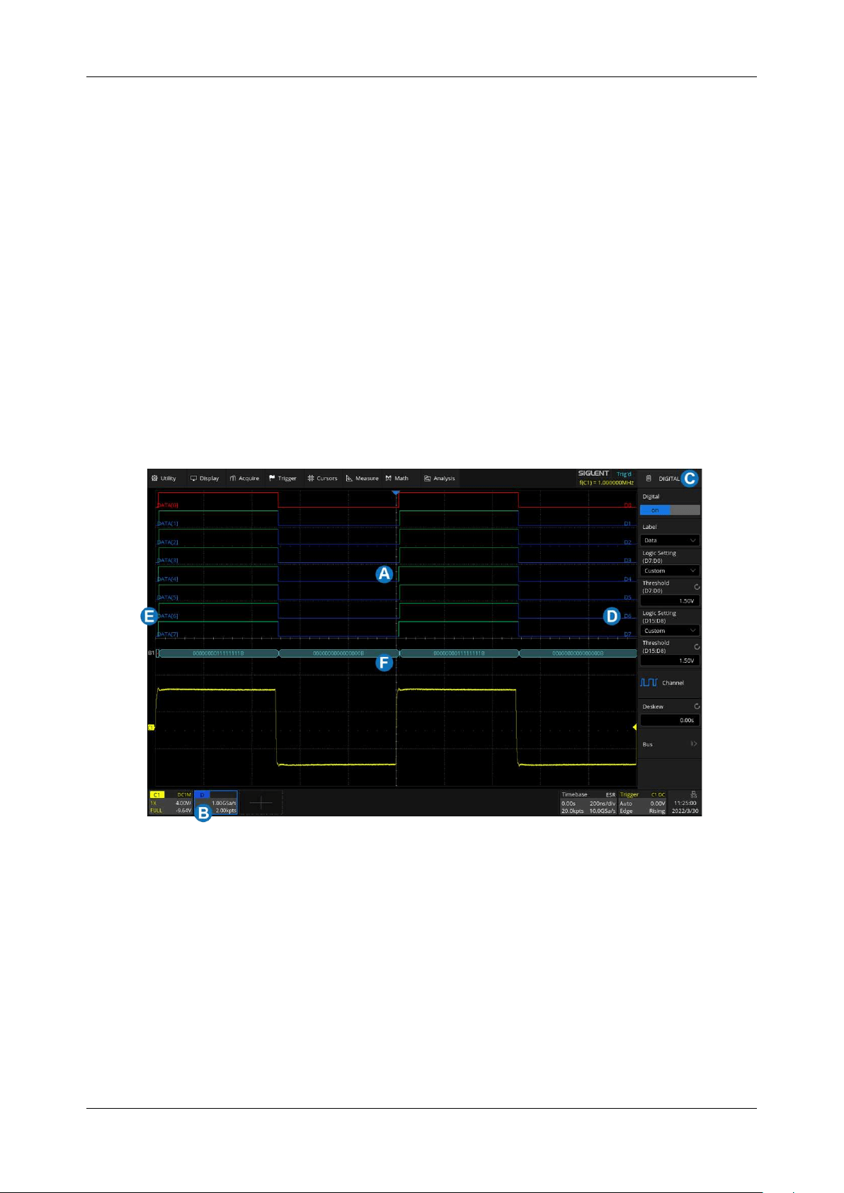
SDS6000L User Manual
int. s i g l e n t . c o m 61
The software option adds the following functions to the oscilloscope:
Digital channel acquisition and analysis
- Acquire and analyze the signals connected to the
digital logic probe, including waveform display, save, parameter measurement, etc.
Trigger on a digital channel
- Trigger with the digital channel as the trigger source, isolating
events of interest.
Decode on a digital channel
- Serial protocol decoding of a digital channel requires the
installation of the serial decode option.
10.2 Enable/Disable the Digital Channels
Turning on or off the digital channels is similar to analog channels. Digital data can be stored as
waveform files. Horizontal cursors and most horizontal measurements also apply to digital waveforms.
A. Digital channel waveform display, which shares the same grid area with the analog channels.
B. Digital channel descriptor box
C. Dialog box
D. Digital channel indicators. Up to 16 digital channels are organized in two groups with different
thresholds: D15~D8 and D7~D0. Every channel can be turned on or off individually.
E. Labels can be set to data, address, or custom characters.
F. Digital bus
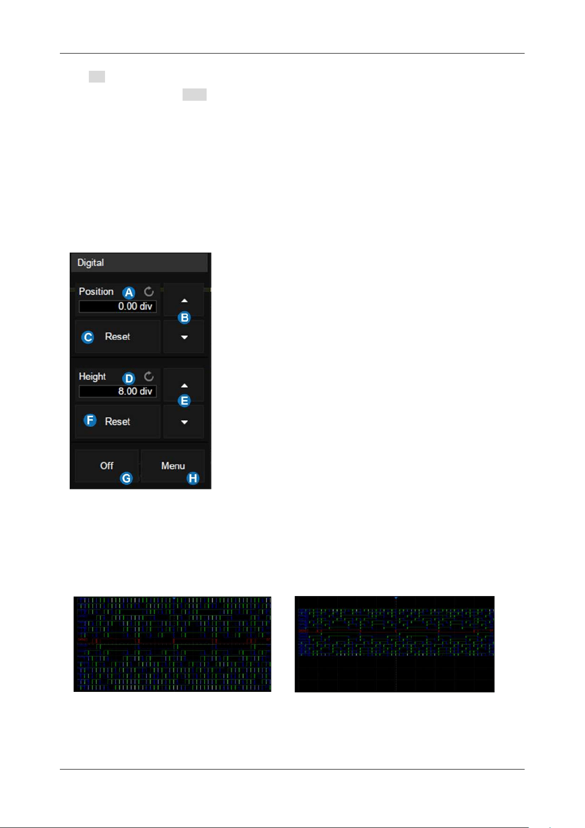
SDS6000L User Manual
62 i n t . s i g l e n t . c o m
Click + at the bottom of the display and select the "Digital" to turn it on. Click the digital channel
descriptor box, and select Off on the pop-up menu to turn it off. Refer to the operation in the chapter
"Vertical Setup" for details.
10.3 Digital Channel Setup
Click the digital descriptor box, then the quick menu of digital channel settings pops up above the
descriptor box. In the menu height and position of digital channels can be set:
A. Upper position limit of the digital channel display area.
Use the mouse wheel or virtual keypad to set it.
Decrease the height to provide more adjustment area.
B. ▲ to increase position and ▼ to decrease the channel
location.
C. Reset the position to the default value
D. The range in height of the digital channels display
area. Use the mouse wheel or virtual keypad to set it.
If the display height covers all of the available
divisions, there will not be room to adjust the position.
E. ▲ to increase and ▼ to decrease the number of
divisions occupied by the digital channels
F. Reset the height to the default value
G. Turn off the digital channels
H. Open the digital dialog box on the right side
Height=8div, Position=0div
Height=4div, Position=1div
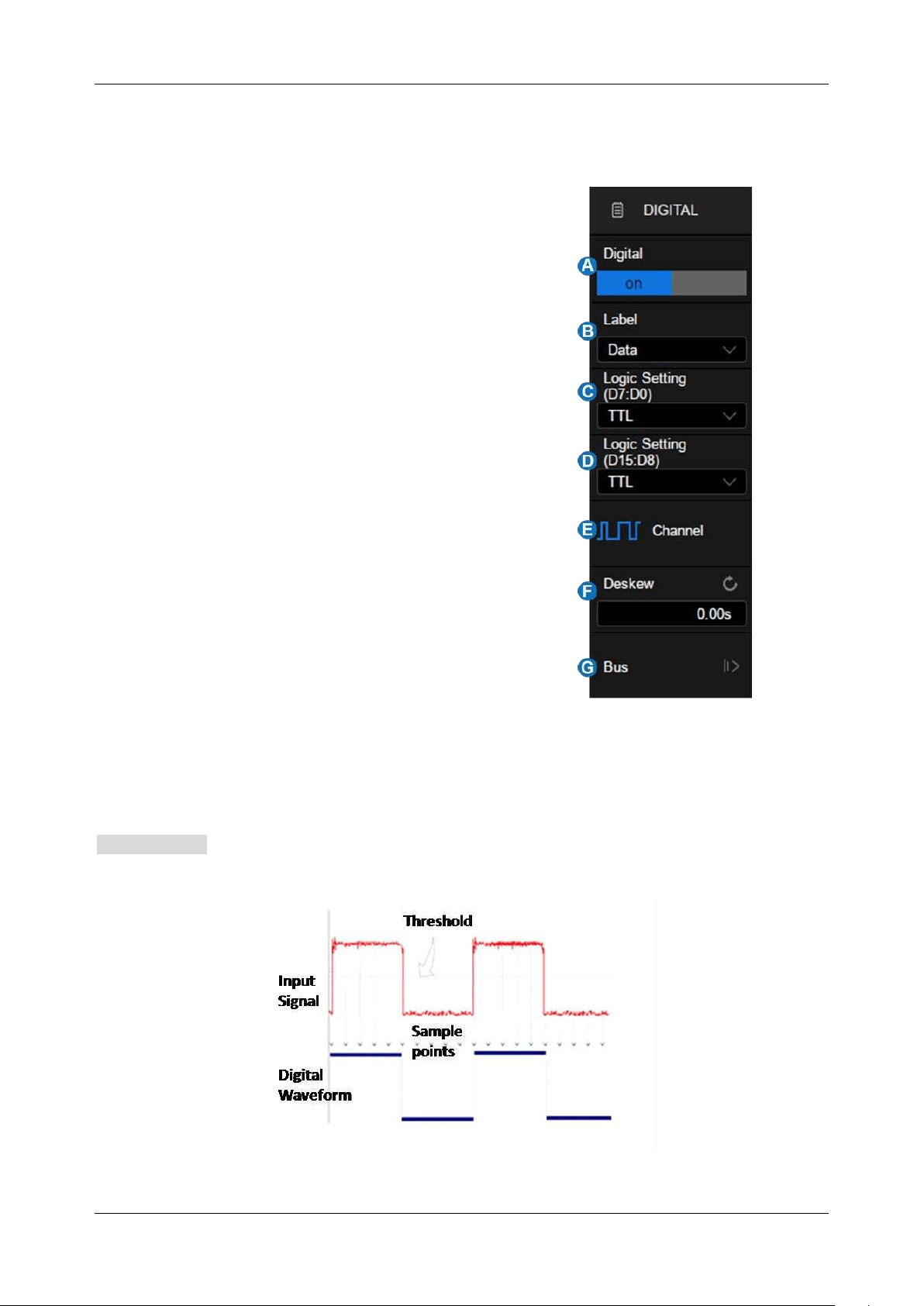
SDS6000L User Manual
int. s i g l e n t . c o m 63
The quick menu only covers the height range and position of the digital channels display area. More
settings can be found in the dialog box.
A. Turn on/off the digital channels
B. Labels can be set to data, address, or custom
characters.
C. Logic threshold of D7~D0. The oscilloscope will
automatically set the threshold according to the
specified logic family, or the user can set the
threshold manually using the Custom option.
D. Logic threshold of D15~D8
E. Set the channels to be displayed
F. Deskew setting, the same as setting analog
channels
G. Bus setting
Logic Threshold Setting
The threshold level determines how the input signal is evaluated. The threshold level can be set in the
Logic Setting . The input voltage less than the threshold is recognized as a '0', and the input voltage
greater than the threshold is recognized as a ‘1’.
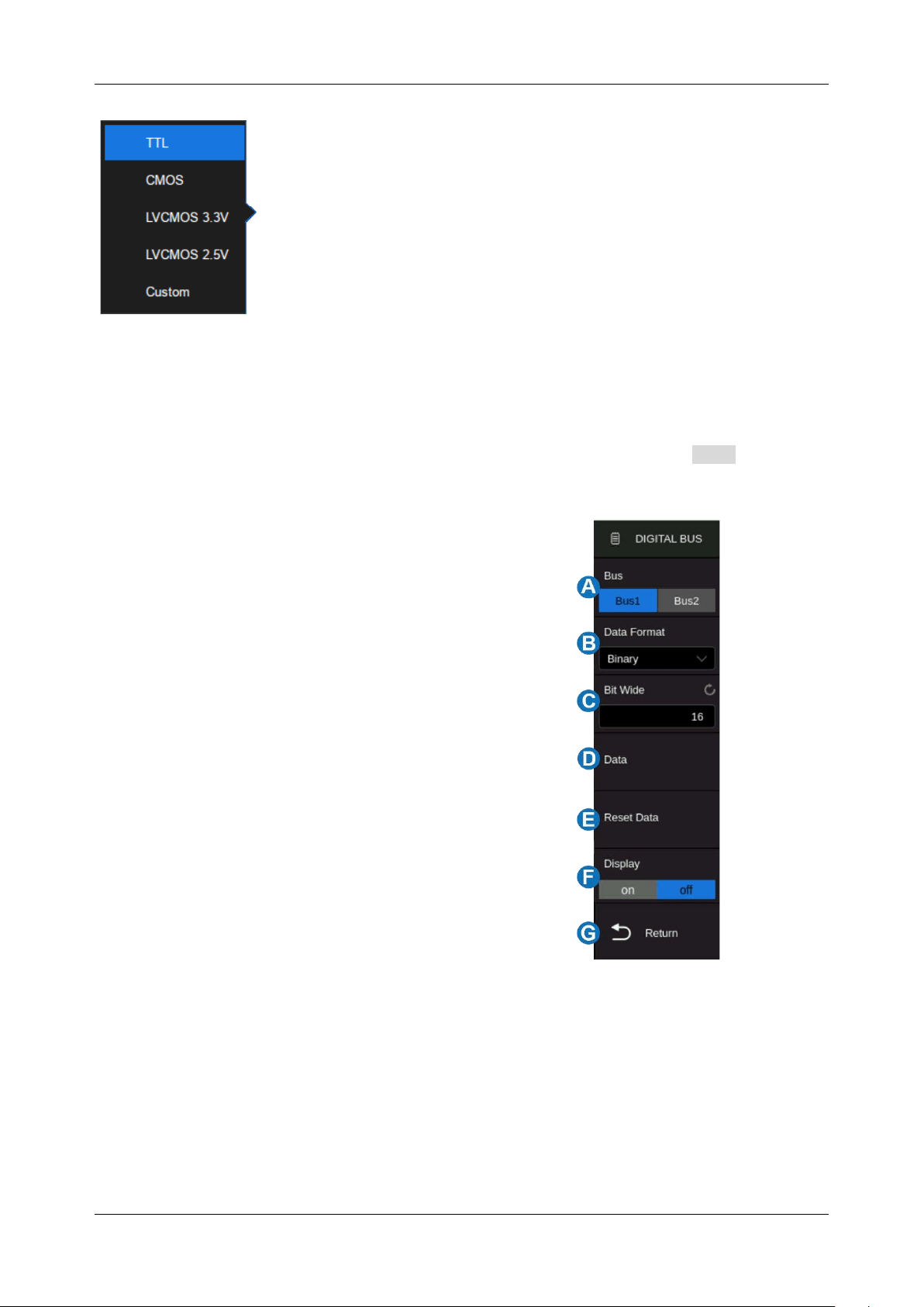
SDS6000L User Manual
64 i n t . s i g l e n t . c o m
The configurable logical level includes TTL, CMOS,
LVCMOS 3.3 V, LVCMOS 2.5 V, and Custom.
The setting range of the custom threshold is - 10.0 V to
+ 10.0 V.
Bus Setting
Click the Digital descriptor box on the bottom to open the Digital dialog box, click Bus to open the
Digital Bus dialog box.
A. Select Bus1 or Bus2
B. Set the data format of the digital bus (binary,
decimal, unsigned decimal, and
hexadecimal)
C. Set the bit width of the digital bus
D. Set the digital bus data
E. Reset the digital bus data to the default state
F. Enable/disable the display of the digital bus
G. Return to the previous menu
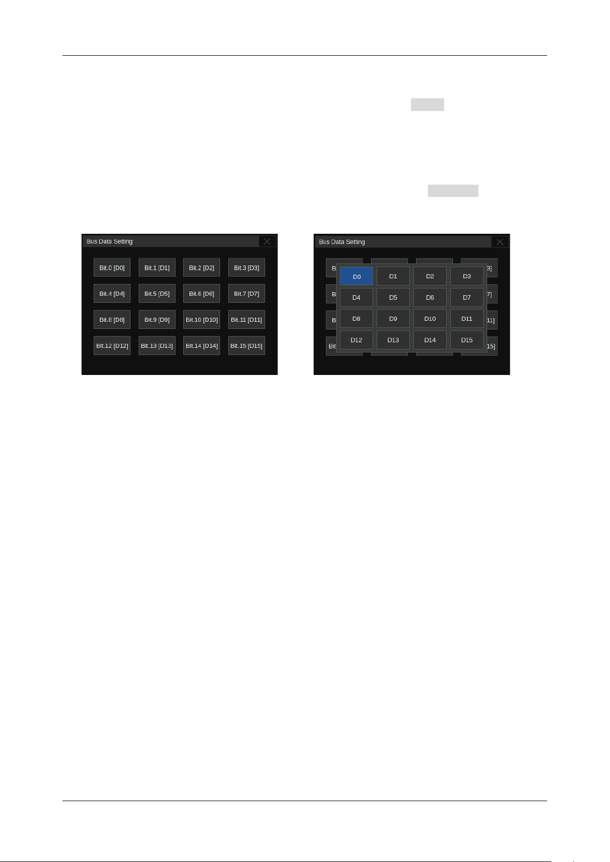
SDS6000L User Manual
int. s i g l e n t . c o m 65
Bus Data Setting
The bus data setting supports setting the digital channel data by bit. Click Data to open the bus data
setting dialog.
In this dialog, the mapping relationship between the bus bits and the digital channels is shown as
Bit.x[Dy]. For example, Bit.0[D15] means that bit 0 of the bus is D15. Click Bit.x[Dy] to assign the
digital channel D0-D15 to the specified bit x.
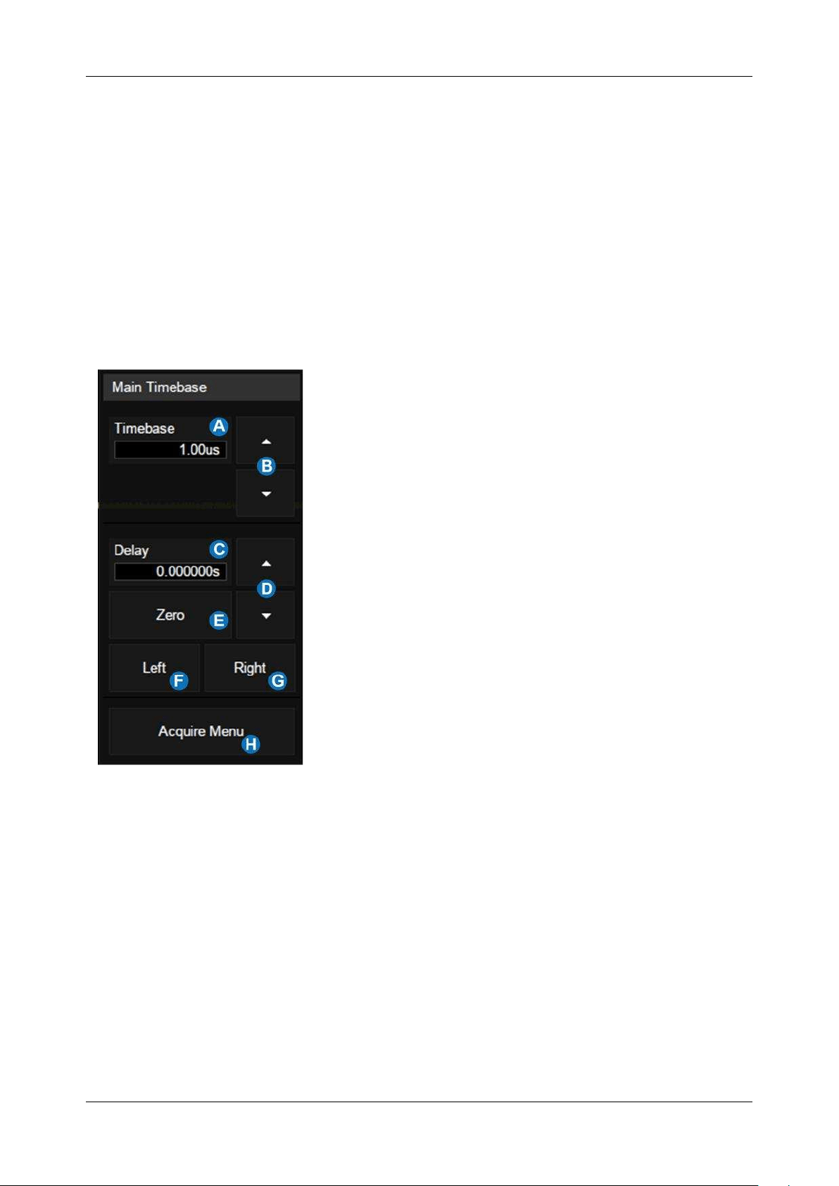
SDS6000L User Manual
66 i n t . s i g l e n t . c o m
11 Horizontal and Acquisition Setup
11.1 Timebase Setup
The timebase setup is used to adjust the scale and offset of the X (horizontal) axis. This setting applies
to all analog, and digital channels as well as all math traces except FFT.
Click the timebase descriptor box and the quick menu of the timebase settings will pop up. In the menu
timebase (horizontal scale), delay and other parameters can be set.
A. Set the horizontal scale (timebase) by the
virtual keypad
B. ▲ to increase and ▼ to decrease the
horizontal scale
C. Set the trigger delay by the virtual keypad
D. ▲ to increase and ▼ to decrease the trigger
delay
E. Set the trigger delay to zero
F. Set the trigger delay to the left part of the
screen
G. Set the trigger delay to the right part of the
screen
H. Open the Acquire dialog box
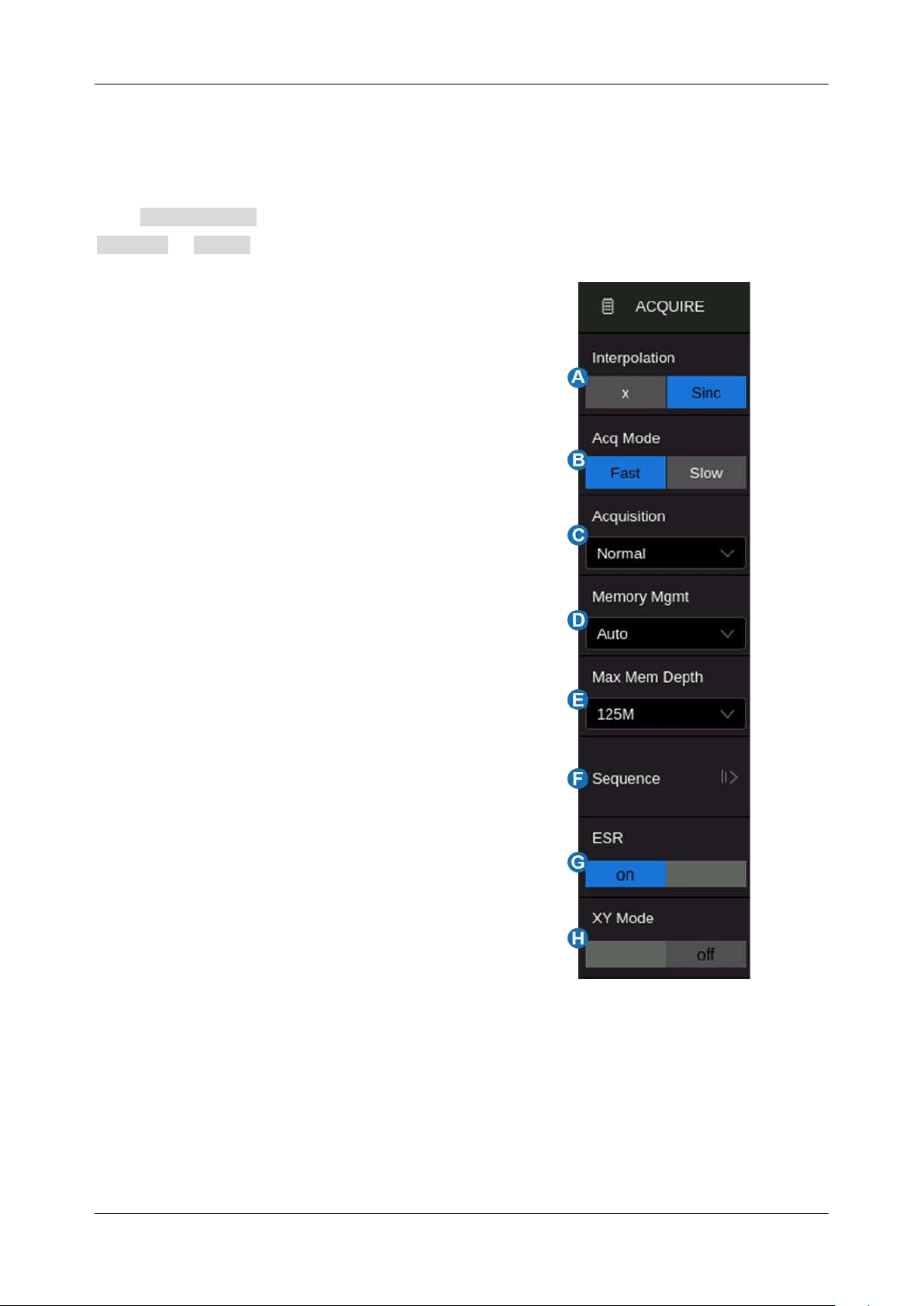
SDS6000L User Manual
int. s i g l e n t . c o m 67
11.2 Acquisition Setup
11.2.1 Overview
Click Acquire Menu on the quick menu of the timebase settings, or click the menu bar
Acquire > Menu to recall the Acquire dialog box on the right side.
A. Select the interpolation mode
B. Select the Acq mode
C. Select the acquisition mode (Normal / Peak /
Average / ERES). See the section "Acquisition"
for details.
D. Select the Memory Management mode (Auto,
Fixed Sample Rate, and Fixed Memory). See
the section "Memory Management" for details.
E. Select the maximum memory depth
F. Enter the sequence menu. See the section
“Sequence” for details
G. ESR mode on/off. See the section “ESR” for
details
H. XY mode on/off
Interpolation
-- At small timebase settings, the number of original points on the screen may be less
than the number of display pixels in the grid area, so interpolation is necessary to display a continuous
waveform. For example, at 1 ns/div timebase and 5 GSa/s sample rate, the number of original points
is 50, but the grid area includes 1250 horizontal pixels. In this case, the oscilloscope needs to
interpolate the original points by 25.
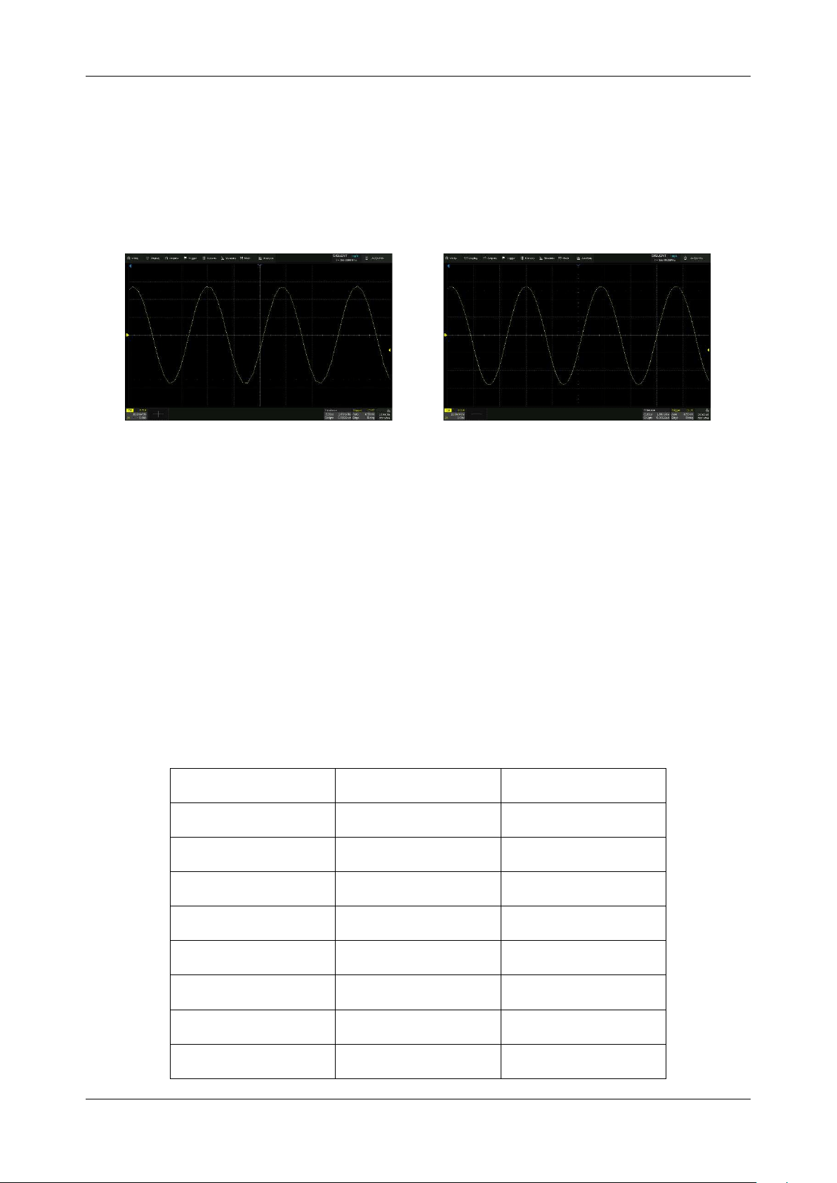
SDS6000L User Manual
68 i n t . s i g l e n t . c o m
X:
Linear interpolation, the simplest way of interpolation, connects two original points with a
straight line.
Sinc
: Sin(x)/x interpolation, the original point is interpolated according to the Nyquist
reconstruction formula, which has a good time-domain recovery effect for a sine wave. But for step
signals / fast rise times, it will introduce false overshoot due to the Gibbs phenomenon.
X Interpolation
Sinc Interpolation
Acq mode:
"Fast" is the default setting. The SDS6000L provides a very high waveform update rate in
fast mode. "Slow" mode will slow down the waveform update on purpose.
Memory Depth
: The memory depth that can be supported. According to the formula "acquisition time
= sample points x sample interval", setting a larger memory depth can achieve a higher sample rate
for a given time base, but more samples require more processing time, degrading the waveform update
rate.
The memory depth supported by the SDS6000L is listed in the following table:
Single Channel Mode
Dual-Channel Mode
Four-Channel Mode
2.5 k
2.5 k
2.5 k
5 k
5 k
5 k
25k
25k
25k
50k
50k
50k
250k
250k
250k
500k
500k
500k
2.5M
2.5M
2.5M
5M
5M
5M

SDS6000L User Manual
int. s i g l e n t . c o m 69
12.5M
12.5M
12.5M
25M
25M
25M
50M
50M
50M
125M
125M
125M
250M
250M
500M
Channels 1, 2, 3, and 4 (C1~C4) are in group 1 and 5, 6, 7, and 8 (C5~C8) are in group 2
Single-channel mode: In one group, only one channel is on and in the other group, one channel
or less is on.
Dual-channel mode: In one group, two channels are turned on and in the other group, two channels
or less are turned on.
Four-channel mode: In any group, three or more channels are turned on.
11.2.2 Acquisition
The acquisition mode is used to determine how to acquire and process the signal.
Normal:
The oscilloscope samples the signal with equal time intervals. For most waveforms, the best
display effect can be obtained using this mode.
Peak:
Peak detect mode. The oscilloscope acquires the maximum and minimum values of the signal
within the sample interval so the peak (maximum-minimum) in the interval is obtained. This mode is
effective to observe occasional narrow pulses or spurs with a low sample rate, but the noise displayed
is larger. In peak mode, the oscilloscope will display all pulses with a pulse width longer than 200 ps.
In the following example, a narrow pulse sequence with a pulse width of 3.4 ns and a period of 200 Hz
is sampled at a 5 MSa/s sample rate in normal mode and peak mode. As we can see, because the
sample interval (200 ns) is much larger than the pulse width (3.4 ns), it is difficult to capture the narrow
pulses in normal mode, but peak mode can ensure that each pulse is captured.
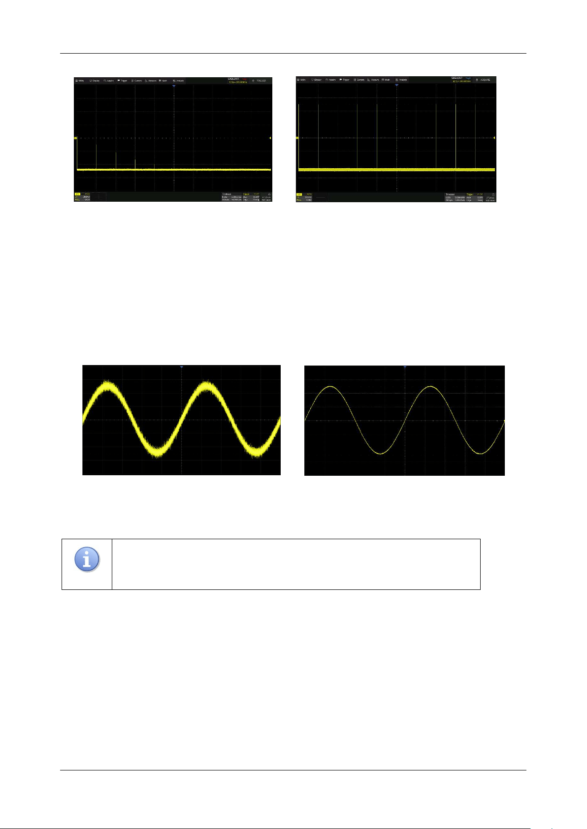
SDS6000L User Manual
70 i n t . s i g l e n t . c o m
Normal mode
Peak mode
Average:
The oscilloscope accumulates multiple waveform frames and calculates the average as the
result. If a stable trigger is available, the resulting average has a random noise component lower than
that of a single-shot record. The more frames that are accumulated, the lower the noise is. For the
SDS6000L, average processing is implemented by the hardware engine, so it can still maintain a high
waveform update rate when the acquisition mode is set to average.
Normal mode
Average mode
(
32
)
Note:
Average acquisition is only valid for periodic signals, and it is important
to ensure that the waveform is triggering stably when using average mode.
ERES:
In this mode, the oscilloscope digitally filters the sampling points, which can reduce the
broadband random noise on the input signal and improve the signal-to-noise ratio, to improve the
effective resolution (ENOB) of the oscilloscope. The ERES processing of the SDS6000L is realized by
the hardware engine, so it can still maintain a high waveform refresh rate when ERES is turned on.
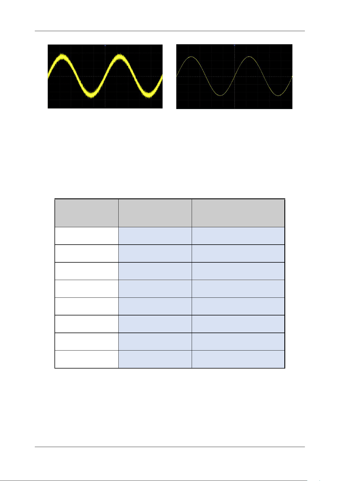
SDS6000L User Manual
int. s i g l e n t . c o m 71
Normal mode
ERES mode (3-bit)
ERES acquisition does not require the signal to be periodic, nor does it require stable triggering, but
due to the digital filtering, the system bandwidth of the oscilloscope will degrade in ERES mode. The
higher the enhanced bits, the lower the bandwidth. The following table shows the relationship between
ERES bits and bandwidth:
Enhanced Bits
Equivalent Hi-Res
Enhanced Resolution
-3dB bandwidth
0.5
1
0.25*Sample rate
1
2
0.115*Sample rate
1.5
3
0.055*Sample rate
2
4
0.028*Sample rate
2.5
5
0.014*Sample rate
3
6
0.007*Sample rate
3.5
7
0.0035*Sample rate
4
8
0.0017*Sample rate
SDS6000L User Manual
72 i n t . s i g l e n t . c o m
11.2.3 Memory Management
Memory Management controls how the instrument stores the acquired samples.
Auto: The default acquisition setting. After setting the maximum memory in the Auto mode, the
oscilloscope automatically adjusts the sample rate and memory depth according to the time base. The
adjustment principle is to follow the formula:
Sample rate = number of samples/time of acquisition
Where the time of acquisition is the time corresponding to the full display (i.e. 10 horizontal divisions).
Note:
The maximum memory here is the upper limit of the memory space
allocated by the oscilloscope. The actual sample points are related to the
current time base and may be less than memory depth. The actual sample
points information can be obtained in the timebase descriptor box (see the
section "Timebase and Trigger" for details).
Fixed Sample Rate: The sample rate is fixed as set, and the oscilloscope automatically adjusts
memory depth according to the time base. The time of acquisition is the time corresponding to the full
display (i.e. 10 horizontal divisions).
Fixed Memory: The memory depth is fixed as set, and the oscilloscope automatically adjusts the
sample rate according to the time base. With a small time scale (such as 1 ns/div) the memory depth
is beyond the time of the full display, so it needs to zoom out the acquired frame for viewing the
complete frame in Stop mode.
Note:
When the status is Run, the scope only processes the data on the
display, which means measure, math, decode, search, etc. only analyzes the
data on the display. This is identical to the "Auto" memory management
mode.
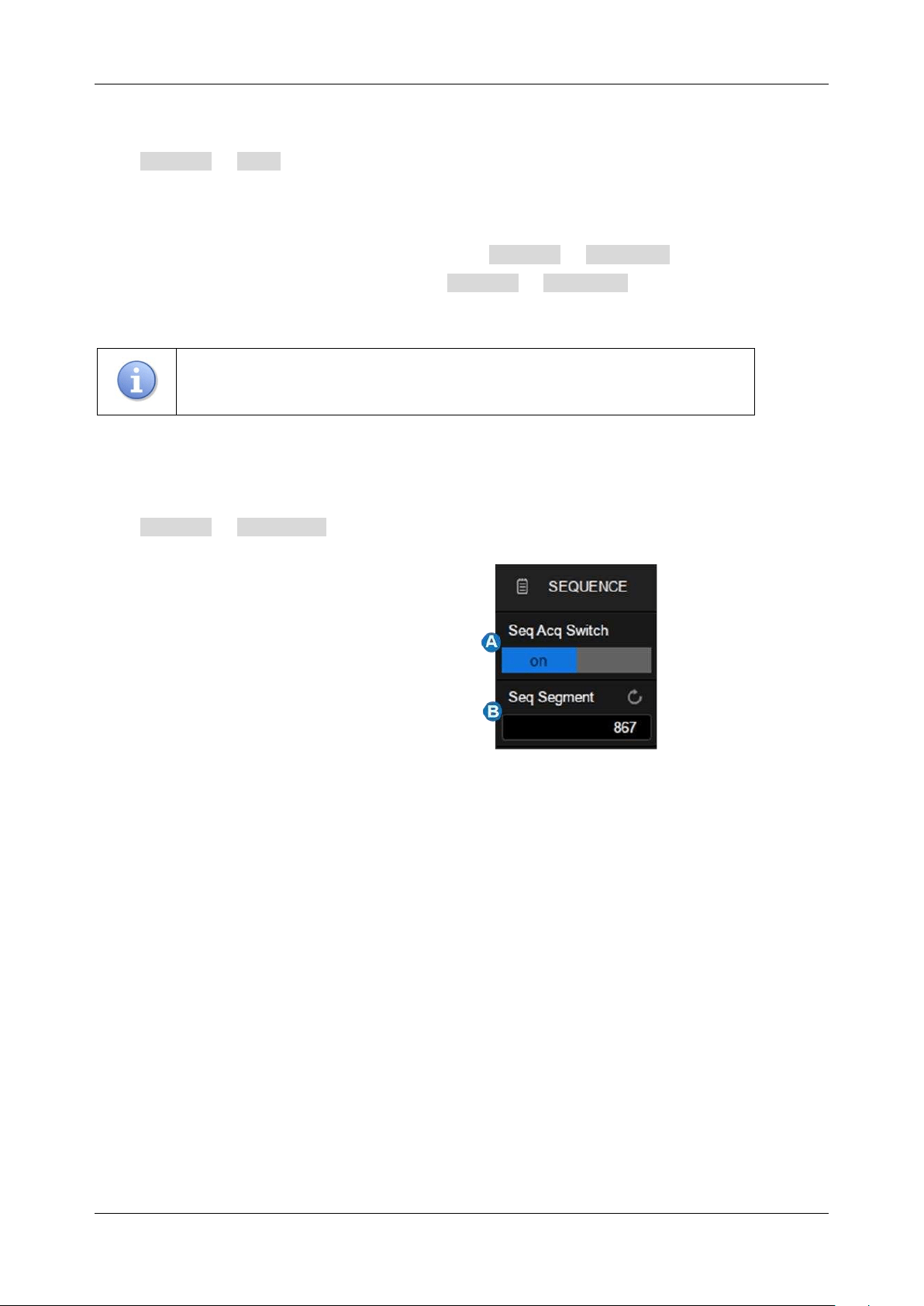
SDS6000L User Manual
int. s i g l e n t . c o m 73
11.2.4 Roll Mode
Click Acquire > Roll to enter roll mode. In this mode, the waveform moves across the screen
from right to left, similar to a strip chart recorder. The horizontal delay control of the waveform will be
disabled when roll mode is active. It only operates at timebase values of 50 ms/div and above.
If you would like to stop the display in Roll mode, click Acquire > Run/Stop . To clear the display
and restart an acquisition in Roll mode, perform Acquire > Run/Stop again.
Note:
Zoom is only supported after Stop in Roll mode.
11.2.5 Sequence
Click Acquire > Sequence to recall the sequence dialog box.
A. Turn on or off sequence
B. Set the segment
Sequence mode is a fast acquisition mode, which divides the memory depth into multiple segments
(up to 80,000), each of which stores a single shot. In sequence mode, the oscilloscope only acquires
and stores data without processing and displaying it until the specified segments are acquired. As a
result, the dead time between trigger events is minimized, thus greatly improving the waveform update
rate. If sequence mode is enabled, the display will not update until all of the sequences have been
acquired. The SDS6000L can achieve a minimum 1.3 us trigger interval in Sequence mode,
corresponding to a waveform update rate of 750,000 wfm/s.
After the acquisition is finished, the oscilloscope will map all the segments together to the screen. If
you need to view and analyze each frame separately, history mode will help (see the section "History"
for details). History mode provides timestamp labels for each segment.
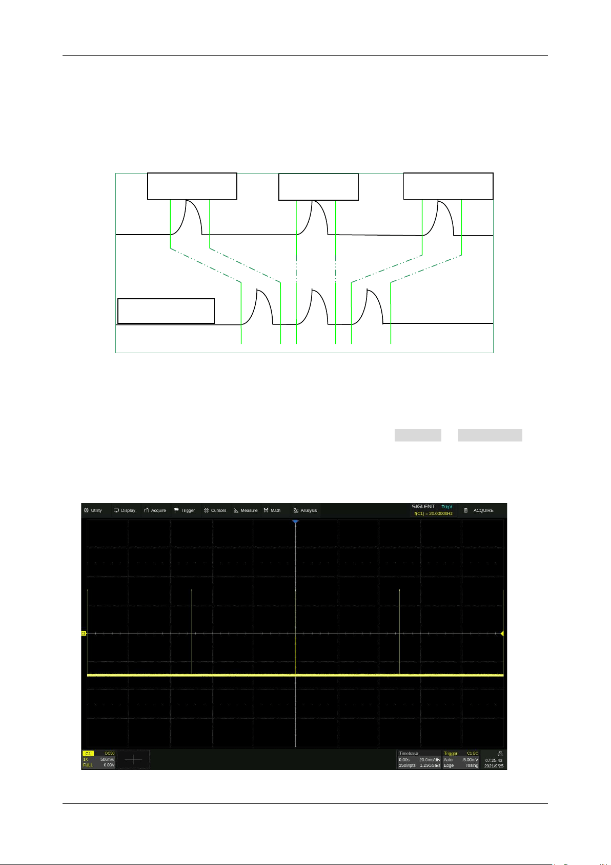
SDS6000L User Manual
74 i n t . s i g l e n t . c o m
In addition to minimizing the dead time, another advantage of Sequence mode is that it can capture
and record rare events over long periods. The oscilloscope can capture multiple events that satisfy the
trigger conditions, ignoring the periods of no interest between adjacent events, thus maximizing the
use of waveform memory. You can use the full accuracy of the acquisition timebase to measure
selected segments.
Example:
Input a pulse sequence with a period of 50 ms to C1. The rise time of the pulse is 2 ns, the fall time is
100 ns, the pulse width is 108 ns, and amplitude is 1.6 Vpp. Perform Acquire > Auto Setup .
Set the coupling mode of C1 to DC50Ω, and vertical scale to 500 mV/div, vertical offset to 0. Set the
trigger level to 0.
Stored Waveform
Sequence N-1
Sequence N
Sequence N+1
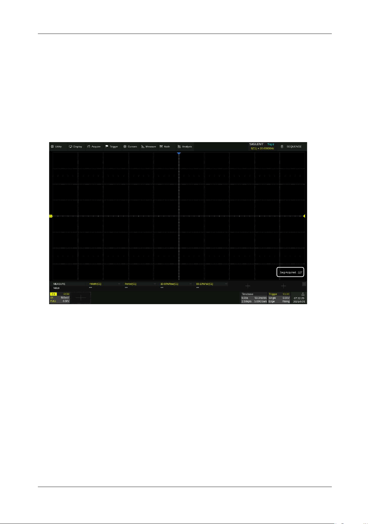
SDS6000L User Manual
int. s i g l e n t . c o m 75
In normal mode, 5 pulses can be obtained on the screen with the sample rate of 1.25 GSa/s
at the maximum memory depth.
Set the trigger mode to "Single" and the timebase to 50 ns/div. Turn on the Sequence mode, and set
the segments to maximum (46,378 in this example, up to 80,000 depending on the number of samples
at the current time base). Wait patiently until the acquisition completes, then all the waveforms
satisfying the trigger conditions are displayed on the screen.
In Sequence mode, there is no waveform displayed on the screen until the acquisition is
completed. During acquisition, there is a counter on the screen indicating the number of
segments that have been acquired.
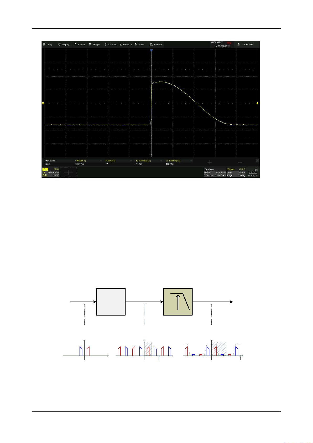
SDS6000L User Manual
76 i n t . s i g l e n t . c o m
In the example, 53969 pulses can be obtained with the sample rate of 5 GSa/s at the
maximum memory depth.
11.2.6 ESR
Each channel of the SIGLENT SDS6000L Oscilloscope employs a 5 GSa/s analog-to-digital-converter
(ADC). After each ADC, a 2x interpolation process is applied that provides a 10 GSa/s ESR option for
the users. The data flow and corresponding spectrum are shown in the figure below:
1
st
Nyquist Zone
1
st
Nyquist Zone
2X
A/D
10 GSa/s
5 GSa/s
Analog
Fs = 5 GSa/s
Fs = 10 GSa/s
ESR data flow in the SDS6000L
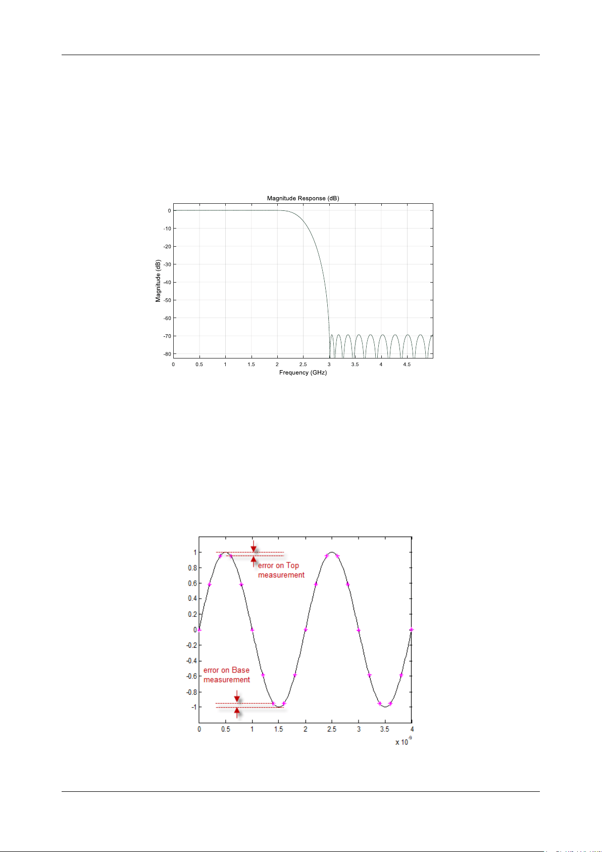
SDS6000L User Manual
int. s i g l e n t . c o m 77
The 2x interpolation implemented is a classic sinx/x up-sampling processed by a high-speed Field
Programmable Gate Array (FPGA) in real-time. The following figure shows the frequency response of
the Finite Impulse Response (FIR) digital filter used in the interpolation. From the frequency response,
we can see it has no attenuation at fmax = 2 GHz, and ~70 dB attenuation at 5 GHz – fmax = 3 GHz,
which provides enough alias suppression for signals in the operating bandwidth. The aliasing
associated with signals above 2 GHz is minimized by the fast roll-off of the analog front end.
Higher measurement precision
The ADC sample rate to bandwidth ratio in the SDS6000L is 2.5:1. That means for a 2 GHz input there
are 2.5 samples/period. Without any extra interpolation, the measurements on vertical waveform
elements such as Maximum, Minimum, and Peak-peak will introduce considerable error at high-
frequency input. The figure below shows an example in which a 500 MHz signal is sampled at 5 GSa/s:
Error on vertical measurement introduced by insufficient sampling
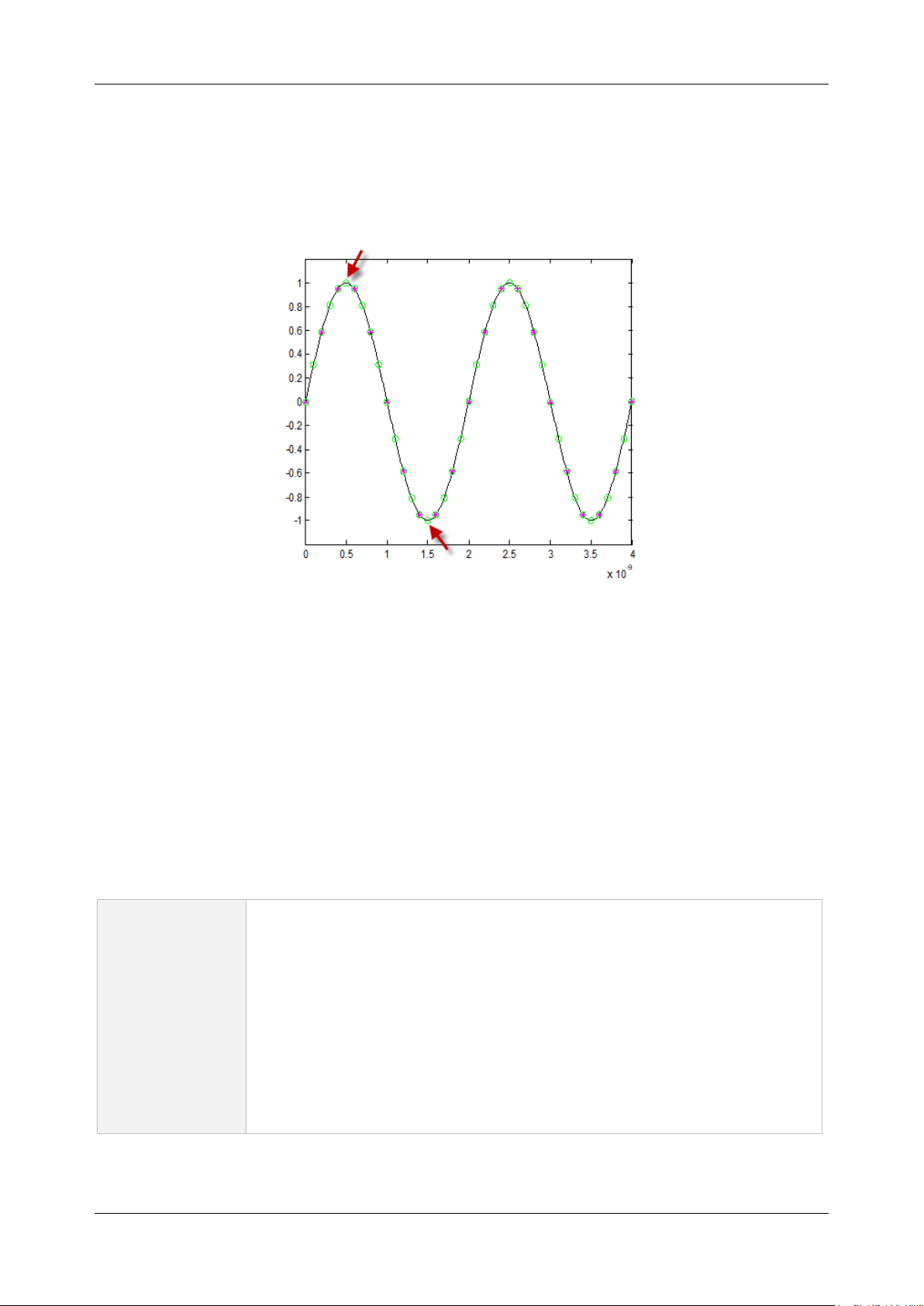
SDS6000L User Manual
78 i n t . s i g l e n t . c o m
Interpolation can significantly reduce this kind of error. Below is the same signal with an identical
sample rate but followed by the 2x interpolation technique. From this figure, we can see points inserted
between the raw data in the top/base area are closer to the real top/base of the analog input, which
reduces the error.
Error on vertical measurement after 2x interpolation
Higher ERES bandwidth
High-resolution acquisition in the SDS6000L enhances the vertical resolution but doing so results in a
decrease in the available bandwidth. The higher the resolution, the lower the bandwidth. The bandwidth
as a function of resolution and sample rate is shown in the table below:
Table: Bandwidth specifications of the SDS6000L in ERES acquisition mode
Bandwidth in
ERES mode
(typical)
0.5-bit: 0.25*Sample rate, up to the analog bandwidth
1-bit: 0.115*Sample rate, up to 1.15 GHz, limited by the analog bandwidth
1.5-bit: 0.055*Sample rate, up to 550 MHz, limited by the analog bandwidth
2-bit: 0.028*Sample rate, up to 280 MHz
2.5-bit: 0.014*Sample rate, up to 140 MHz
3-bit: 0.007*Sample rate, up to 70 MHz
3.5-bit: 0.0035*Sample rate, up to 35 MHz
4-bit: 0.0017*Sample rate, up to 17 MHz

SDS6000L User Manual
int. s i g l e n t . c o m 79
With the ESR enabled, in ERES acquisition mode, the bandwidth will be twice as scenarios without
ESR:
Table: ERES Bandwidth comparison between ESR disabled and enabled
Enhanced
Resolution
Bandwidth with ESR = OFF
(5 GSa/s)
Bandwidth with ESR = ON
(10 GSa/s)
0.5-bit
1.25 GHz
2 GHz
1-bit
575 MHz
1.15 GHz
1.5-bit
275 MHz
550 MHz
2-bit
140 MHz
280 MHz
2.5-bit
70 MHz
140 MHz
3-bit
35 MHz
70 MHz
3.5-bit
17.5 MHz
35 MHz
4-bit
8.5 MHz
17 MHz
Limitations
The ESR algorithm has its limitations. It cannot enhance the hardware performance of an ADC and
introduces extra overshoot/undershoot and ringing on fast edges.
With this understanding, the user can choose to enable ESR or not, according to the actual application.
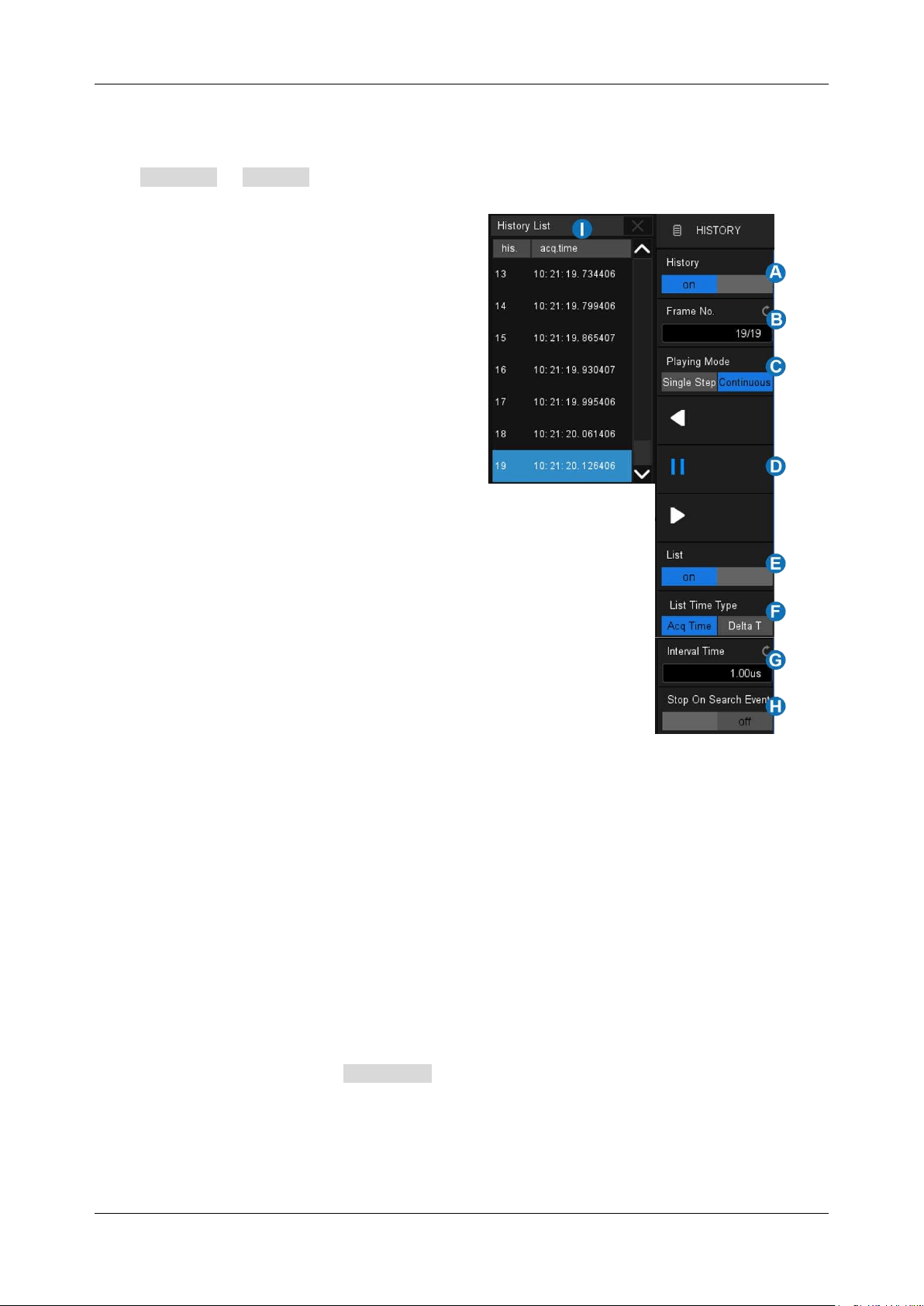
SDS6000L User Manual
80 i n t . s i g l e n t . c o m
11.3 History
Click Analysis > History to recall the history dialog box.
A. Turn on or off history mode
B. Specify the frame index
C. Set the playing mode
D. Play backward, pause, and play forward
E. Turn on or off the list
F. List time type
G. Set the time interval between two frames
when playing automatically
H. Enable the “Stop on Search Event”
function, which allows navigating search
events across history frames.
I. List displays the frame index and time
label for each frame.
The oscilloscope automatically stores acquired frames. It can store up to 80,000 frames but the number
may vary due to the memory depth and timebase settings. Turn on history mode, then the stored
frames can be recalled and measured.
Continue with the example in the section above. In Sequence mode, all waveforms that satisfy the
trigger conditions are mapped to the display. If you need to observe a single frame, you can use history
mode.
To enable history mode, click the Frame No . area twice, then the virtual numeric keypad pops up.
Input the number "5412" to specify the 5412th segment (frame).
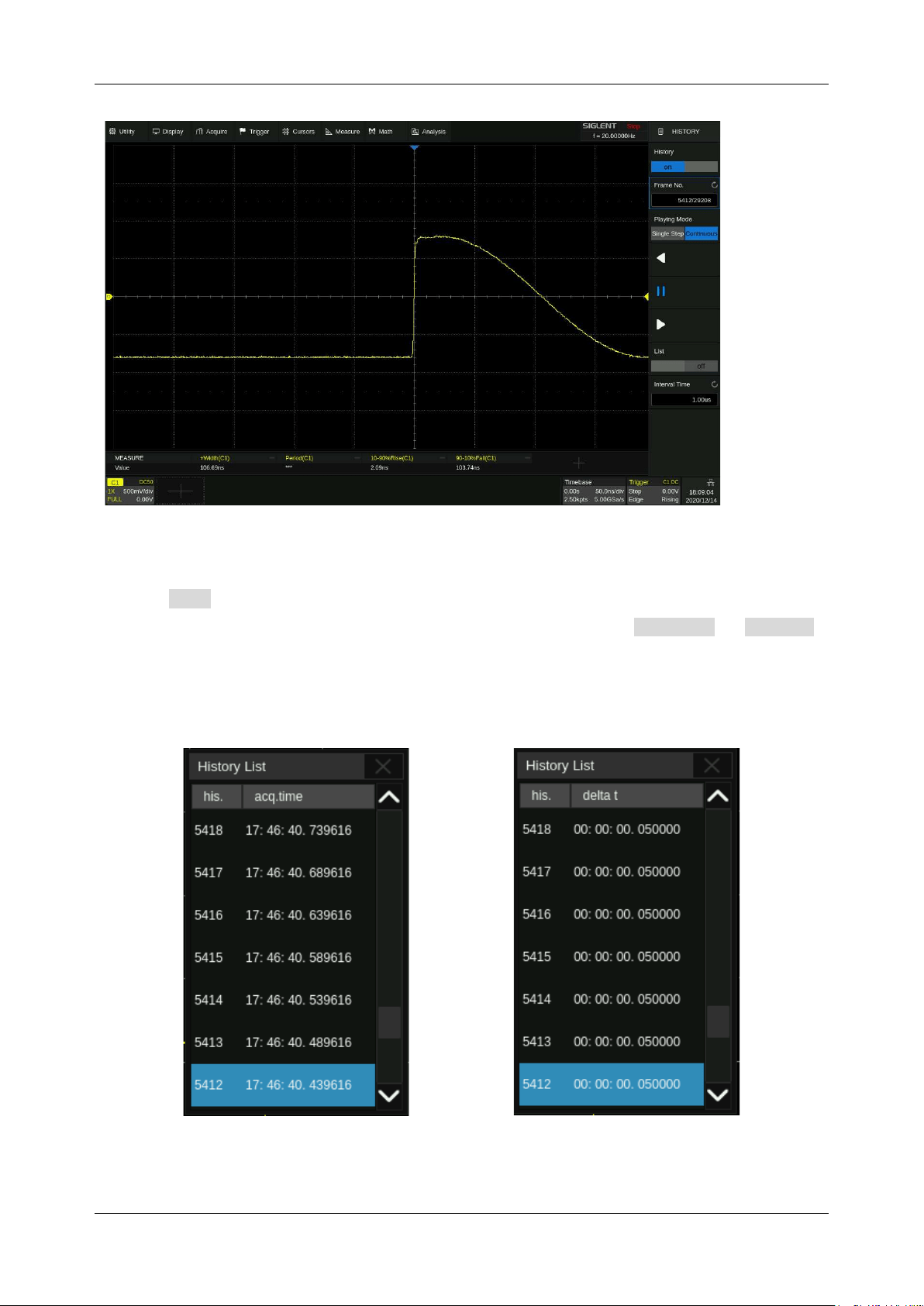
SDS6000L User Manual
int. s i g l e n t . c o m 81
Observing the 5412th frame captured by Sequence in history mode
Click the List area and turn on the list. The time label corresponding to the 5412th waveform is
displayed. The time resolution is microseconds. Time label types include AcqTime or Delta T ,
AcqTime corresponds to the absolute time of the frame, synchronized with the real-time clock of the
oscilloscope; Delta T is the acquisition time interval between adjacent two frames, it is shown as 50ms
in the following diagram, which is consistent with the period of the actual waveform.
Acq Time label
Delta T label
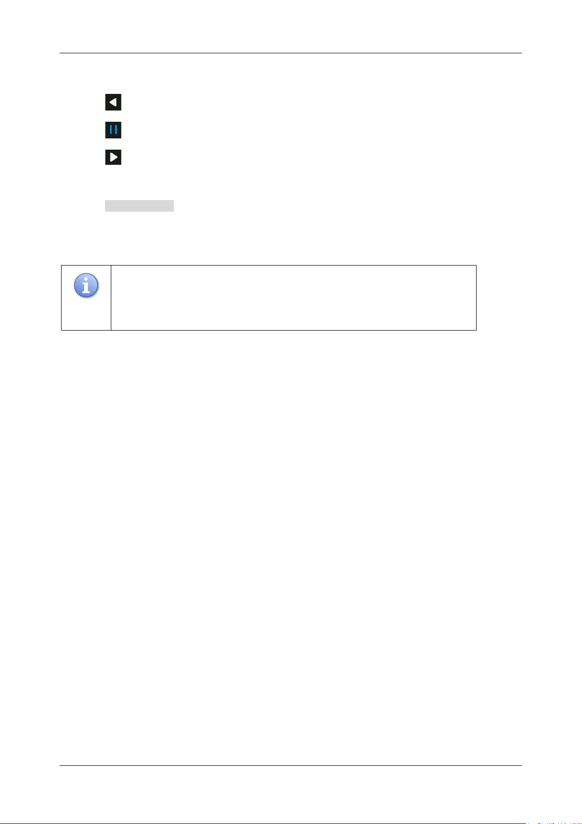
SDS6000L User Manual
82 i n t . s i g l e n t . c o m
In addition to manually specifying a frame, history mode supports auto-play:
Click the softkey to replay the waveform from the current frame to the first.
Click the softkey to stop replay.
Click the softkey to replay the waveform from the current frame to the last.
Click the Interval Time area to control the speed of automatic play. In the process of automatic play,
the list will automatically scroll to the current frame.
Note:
When a measurement is enabled in history mode, if the Interval Time is
set to small (e.g. in us) the speed of automatic play may not meet the setting,
because measurements may take longer for each frame.
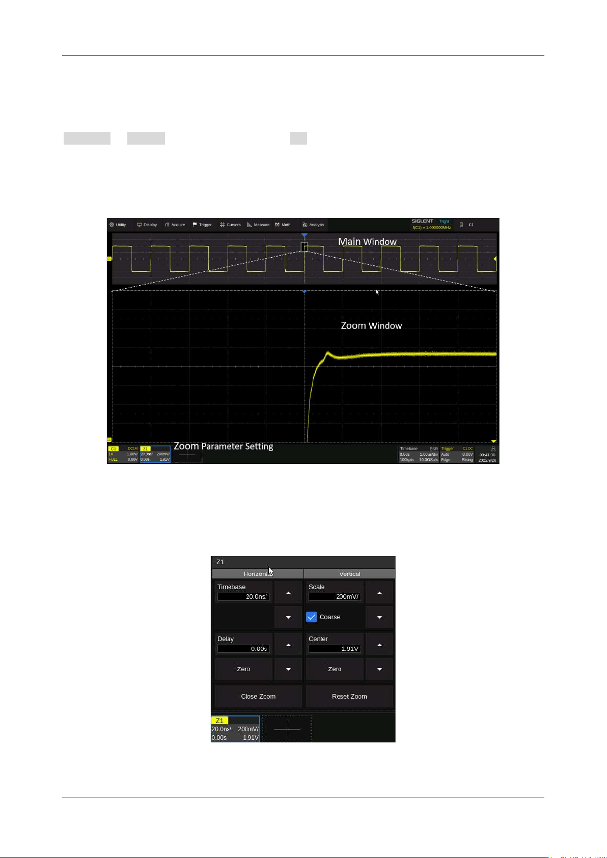
SDS6000L User Manual
int. s i g l e n t . c o m 83
12 Zoom
The SDS6000L supports waveform zoom in the horizontal and vertical directions. Perform
Acquire > Zoom to turn on Zoom, or click + at the bottom to add a zoom trace.
When the Zoom function is on, the waveform area is divided into upper and lower parts. The area of
about 1/3 height above is the main window, and the area of about 2/3 height below is the zoom window.
Click a window to activate it.
The area not covered by the gray background in the main waveform area is the range to be zoomed
in (zoom area). Click the descriptor box of the zoom trace to recall the quick dialogs for setting the
vertical and horizontal parameters of the zoom window.
Horizontal and vertical setting
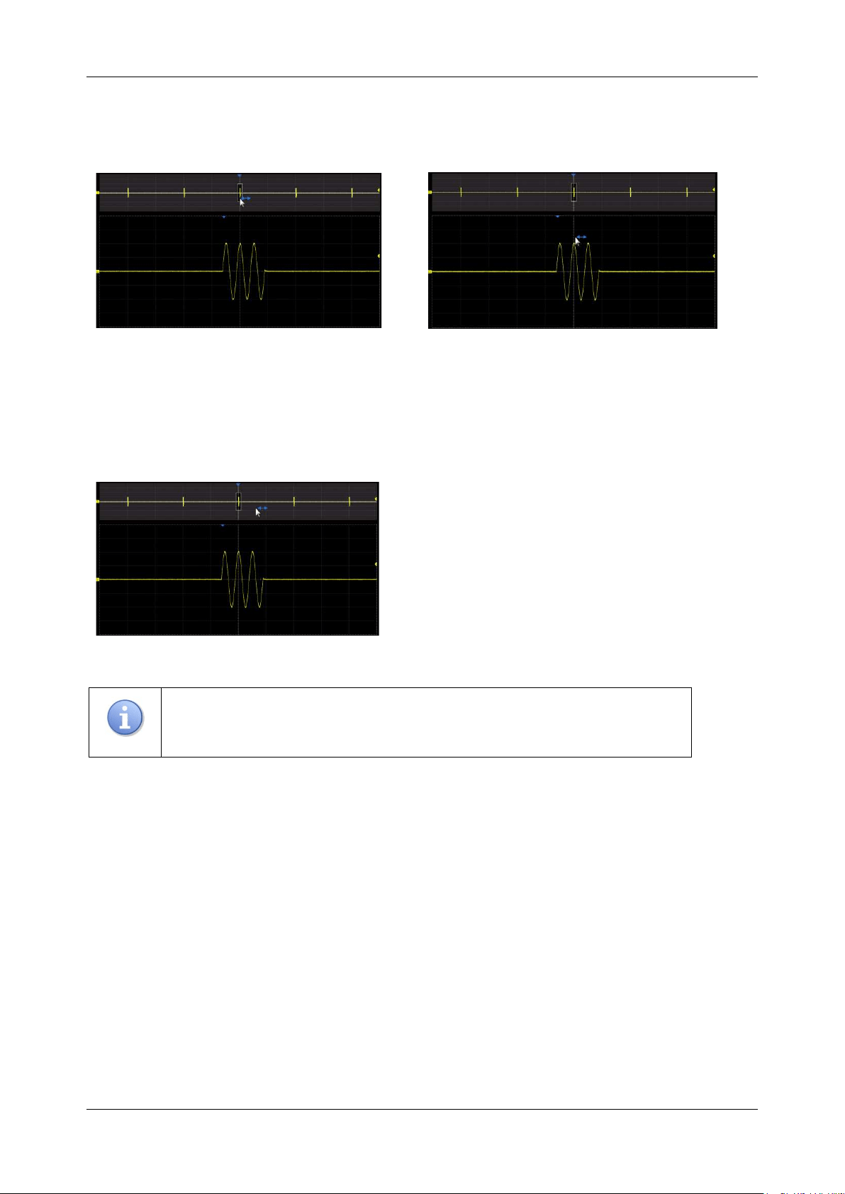
SDS6000L User Manual
84 i n t . s i g l e n t . c o m
Below is an example of changing the setting in the horizontal direction by different actions. The actions
for changing the setting in the vertical direction are similar.
Adjust the horizontal position of the zoom area by dragging left and right in the zoom area of the
main window or waveform in the Zoom window.
Adjust the vertical position of the zoom area by dragging up and down in the zoom area of the
main window or waveform in the Zoom window.
Adjust the horizontal position of the waveform
by dragging the gray area of the main window
left and right.
Adjust the vertical position of the waveform by
dragging the gray area of the main window up
and down.
Note:
Zoom traces (Z1~Z8) can be used as the source of Measurement,
Math, Mask Test, and Histogram.
SDS6000L User Manual
int. s i g l e n t . c o m 85
13 Trigger
13.1 Overview
The oscilloscope only acquires waveforms of interest (i.e. the ones that satisfy the trigger condition)
and aligns all trigger events at the trigger position to form a stable waveform display. The trigger is one
of the most important features of an oscilloscope since we can only analyze a signal that we can trigger
reliably and stably.
The trigger position is movable on the display. The following diagram shows the structure of the
acquisition memory. The acquisition memory is divided into pre-trigger and post-trigger buffers and the
boundary between them is the trigger position. Before the trigger event arrives, the oscilloscope fills
the pre-trigger buffer first, and then continuously updates it in FIFO mode until the trigger event arrives.
After the trigger event, the data fills the post-trigger buffer. When the post-trigger buffer is full, an
acquisition is completed.
Below is the definition of the states in the process of filling the acquisition memory:
Arm:
The pre-trigger buffer is not full, and the oscilloscope does not respond to any trigger events.
Ready:
The pre-trigger buffer is full, and the oscilloscope is waiting for the trigger event.
Trig’d:
A trigger event is detected and the oscilloscope starts to fill the post-trigger buffer.
Trigger settings should be based on the features of the input signal. For example, a sine wave with a
repeatable period can be triggered on the rising edge; for capturing hazards in a combinational logic
circuit, the pulse trigger can be set. You need to have some knowledge of the signal-under-test to
quickly capture the desired waveform.
Pre-trigger Buffer
Post-trigger Buffer
Trigger Event
Acquisition Memory
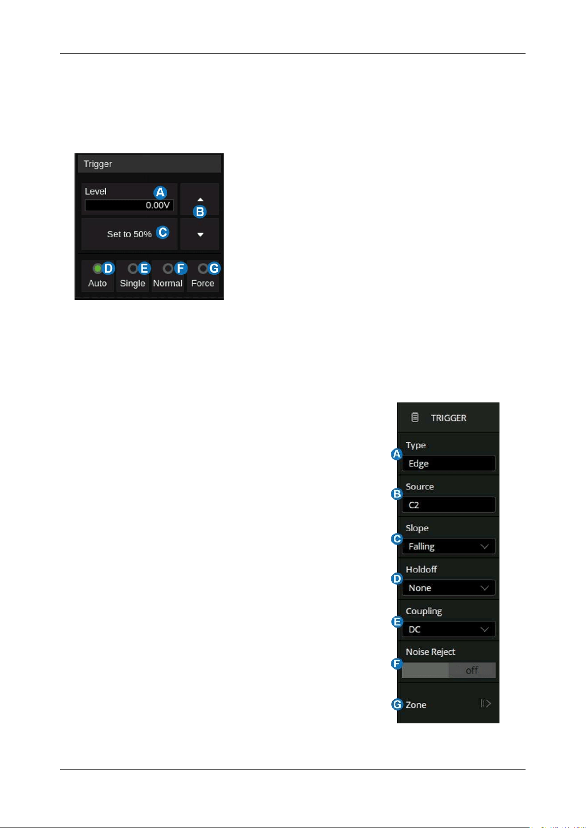
SDS6000L User Manual
86 i n t . s i g l e n t . c o m
13.2 Trigger Setup
Click the trigger descriptor box to display the quick menu of trigger settings. The trigger setup dialog
box is displayed on the right side of the screen.
Quick menu
A. Click the level region and roll the mouse wheel to
adjust the trigger level. Click the region again and
the virtual keypad will be available
B. ▲ to increase and ▼ to decrease the trigger level
C. Set the trigger level to the vertical center of the
waveform automatically
D. Set the trigger mode to "Auto"
E. Set the trigger mode to "Single"
F. Set the trigger mode to "Normal"
G. Perform a force trigger
Trigger setup dialog box:
A. Select trigger type
B. Select the trigger source
C. Select the trigger slope (When the trigger type is
"Edge", "Slope" and other specific types)
D. Set holdoff (None/Time/Events)
E. Set trigger coupling mode (DC/AC/LF Reject/HF
Reject)
F. Enable/disable Noise Rejection. When Noise
Reject is on, the trigger hysteresis is increased,
so the noise immunity of the trigger circuit is
better. As a compromise, the trigger sensitivity
degrades
G. Set the Zone trigger
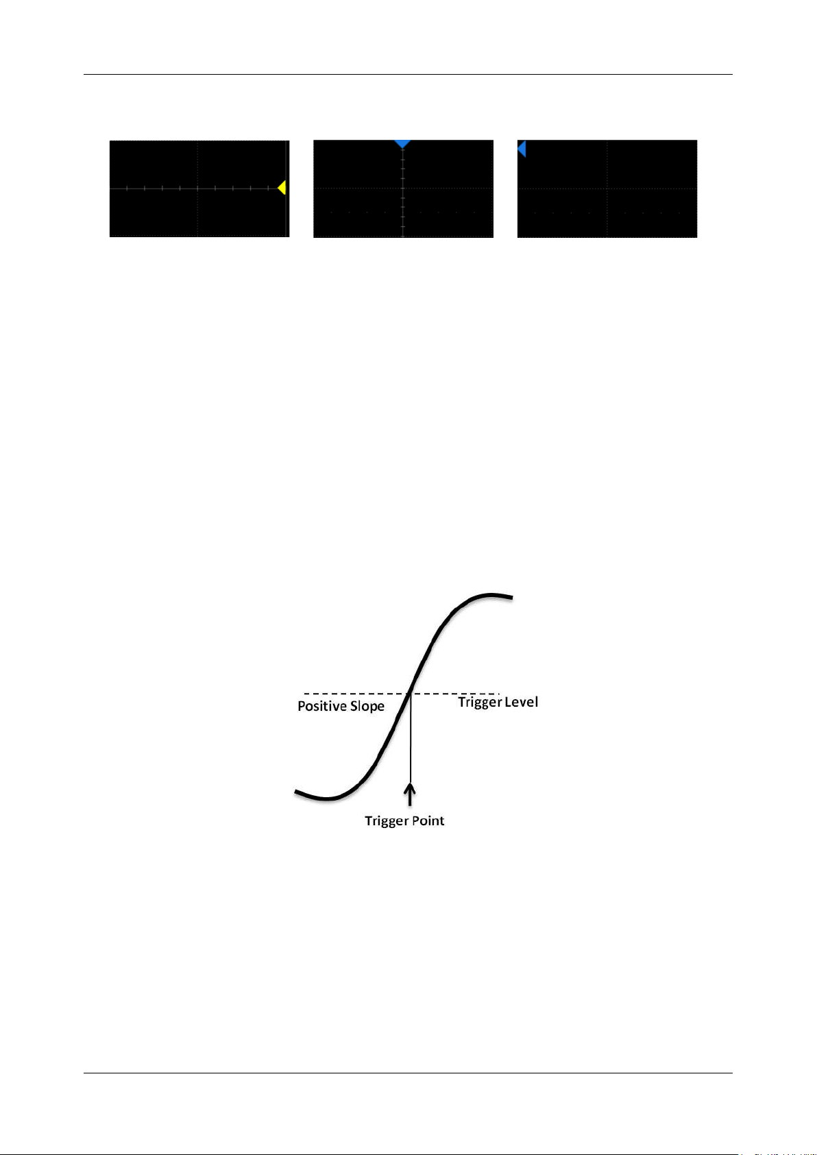
SDS6000L User Manual
int. s i g l e n t . c o m 87
Trigger Related Label
Trigger level Indicator
Horizontal 0 position Indicator
Horizontal 0 position
(out of screen) Indicator
13.3 Trigger Level
Both analog and digital triggers must have a correct trigger level value. The oscilloscope judges
whether a waveform satisfies the trigger condition when it crosses the trigger level. If it does, the
crossing time is the trigger position. In the following figure, the trigger condition is set as a rising edge.
When the signal with a positive slope crosses the trigger level, the trigger condition is satisfied and the
time point the signal crosses the level is the trigger position.
In some special triggers, the system will automatically set the trigger level, such as using AC Line as
the trigger source.
SDS6000L User Manual
88 i n t . s i g l e n t . c o m
13.4 Trigger Mode
The trigger mode determines how the oscilloscope acquires waveforms.
Auto:
An internal timer triggers the sweep after a preset timeout period if no trigger has been found
so that the oscilloscope continuously updates the display whether a trigger happens or not. Auto
mode is suitable for unknown signals or DC signals.
Note:
In Auto mode, if the signal satisfies the trigger conditions but cannot
trigger the oscilloscope stably, it may be that interval between two trigger
events exceeds the timeout period. Try Normal mode in this case.
Normal:
Triggers and acquisitions only occur when the trigger conditions are met. Otherwise, the
oscilloscope holds the last waveform on the display and waits for the next trigger. Normal mode is
suitable for acquiring:
Only events specified by the trigger settings
Rare events
Single:
Captures and displays a single frame that satisfies the trigger conditions, and then stops. The
following trigger events are ignored until the Single acquisition is restarted. Single-mode is suitable for:
One-shot events or periodic signals, such as power-on\off waveforms on a power rail
Rare events
Force:
The oscilloscope triggers regardless of whether the input signal meets the trigger conditions or
not.
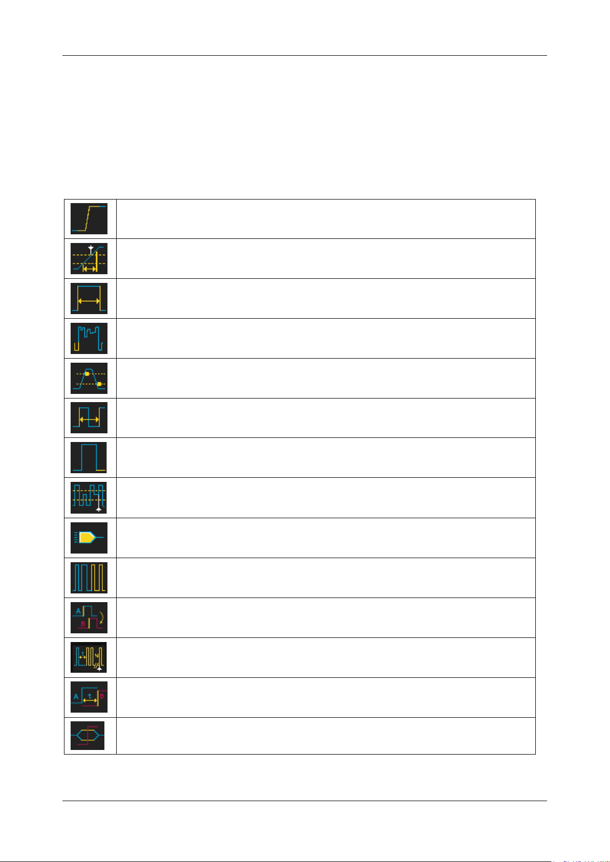
SDS6000L User Manual
int. s i g l e n t . c o m 89
13.5 Trigger Type
13.5.1 Overview
The trigger modes of the SDS6000L are digital designs. Compared with analog trigger circuits, digital
triggers can not only greatly optimize trigger precision and trigger jitter, but also support multiple trigger
types and complex trigger conditions.
Edge
-- Trigger on a rising edge, falling edge or both
Slope
-- Trigger when an edge crosses two thresholds that lie inside or outside a
selected time range
Pulse
-- Trigger at the end of a pulse when the pulse width lies inside or outside a
selected time range
Video
-- TV trigger on falling edge
Window
-- Trigger when the signal leaves the widow region.
Interval
-- Trigger on the second edge when the time between the edges is inside or
outside a selected time range
Dropout
-- Trigger when the signal disappears for longer than the Dropout value.
Runt
-- Trigger when a pulse crosses the 1st threshold but not the 2nd before re-
crossing the 1st threshold again
Pattern
-- Trigger when pattern condition transitions from false to true. All inputs set
to DC coupling
Serial
--Trigger on specified condition in a serial bus. See the chapter "Serial Trigger
and Decode" for details.
Qualified
-- Trigger with edge trigger setting only after the qualifying condition is
satisfied
Nth Edge
–Trigger on the Nth edge of a burst that occurs after a specified idle time
Delay
--Trigger when the delay time between source A and source B meets the limit
condition
Setup/Hold
--Trigger when the setup time or hold time meets the limit condition
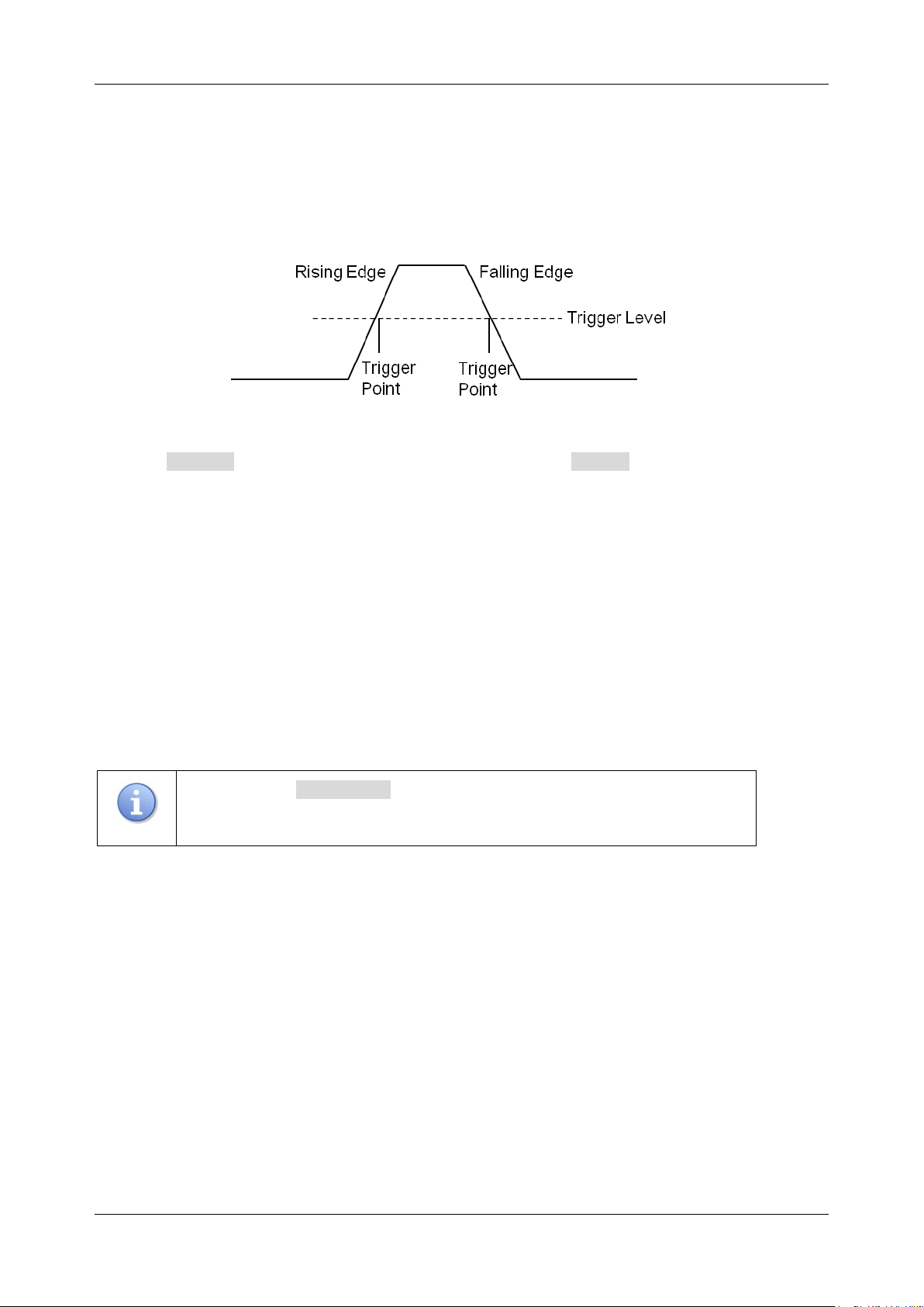
SDS6000L User Manual
90 i n t . s i g l e n t . c o m
13.5.2 Edge Trigger
Edge trigger distinguishes the trigger points by seeking the specified edge (rising, falling, alternating)
and trigger level. The trigger source and slope can be set in the trigger dialog box.
Click the Source area to select the trigger source, and click the Slope area to select rising, falling,
or alternating.
Rising
-- Only trigger on the rising edge
Falling
-- Only trigger on the falling edge
Alternating
-- Trigger on both the rising and falling edge
Holdoff, coupling, and noise reject can be set in edge trigger, see the sections "Holdoff", "Trigger
Coupling" and "Noise Reject" for details.
Note:
Perform Auto Setup , and the oscilloscope will set the trigger type to
Edge.
13.5.3 Slope Trigger
The slope trigger looks for a rising or falling transition from one level to another level in the specified
time range. For example, positive slope time is defined as the time difference between the two crossing
points of trigger level lines A and B with the positive edge as shown in the figure below.
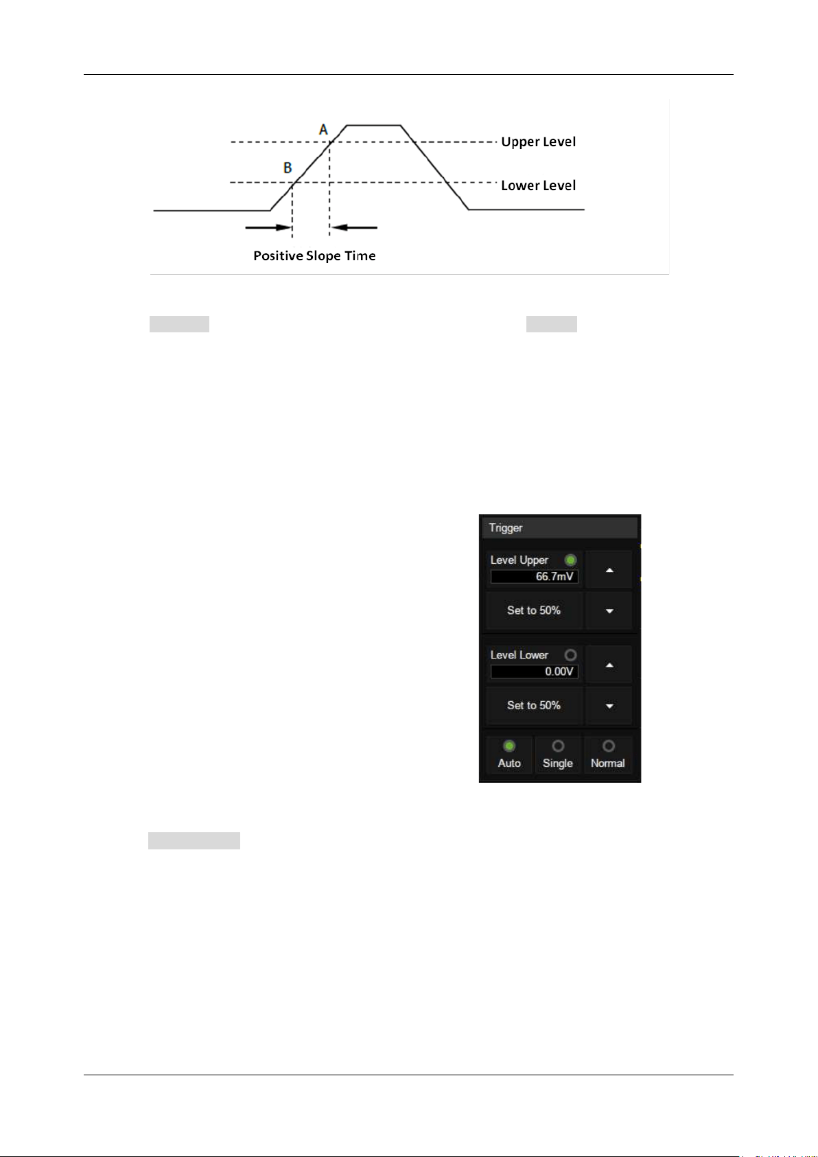
SDS6000L User Manual
int. s i g l e n t . c o m 91
Click the Source area to select the trigger source, and click the Slope area to select rising or
falling.
Rising
-- Only trigger on the positive slope
Falling
-- Only trigger on the negative slope
Adjust the Upper/Lower Level
The slope trigger requires upper and lower trigger
levels. When the trigger type is slope trigger, click
the trigger descriptor box, the pop-up quick menu
will show two levels.
The upper/lower level can be set in the following
way:
Click the Level Upper area in the quick menu to select the upper level, and then set the level value
by the virtual keypad or the mouse wheel. To set the lower level is similar.
The lower level should always be less than or equal to the upper level. In the trigger descriptor box,
the lower level is displayed.
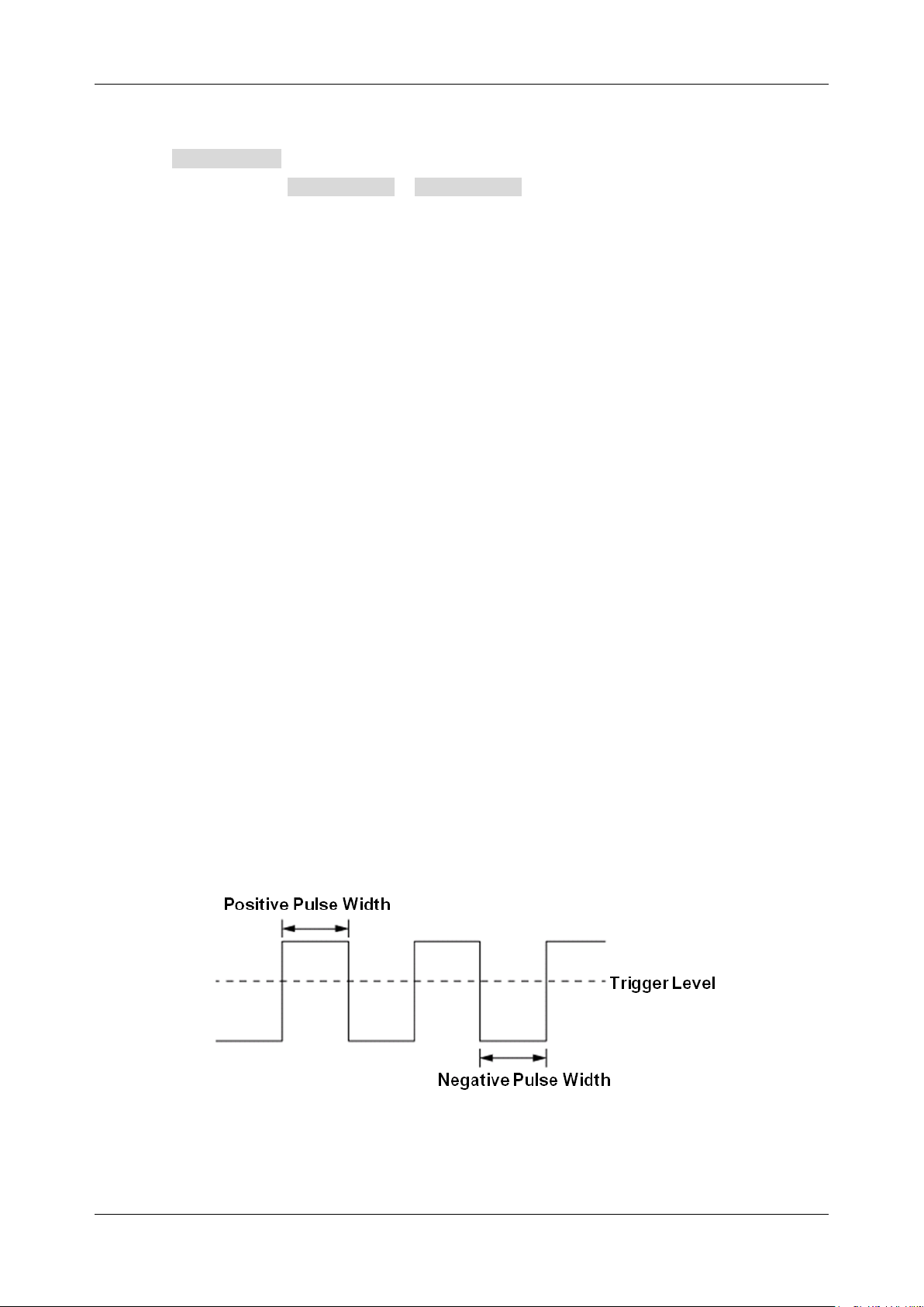
SDS6000L User Manual
92 i n t . s i g l e n t . c o m
Set Limit Range
Click the Limit Range area in the trigger dialog box to select the time condition and set the
corresponding time in the Upper Value / Lower Value area.
Less than a time value
(
≤
)
-- Trigger when the positive or negative slope time of the input signal is
lower than the specified time value.
Great than a time value
(
≥
)
-- Trigger when the positive or negative slope time of the input signal
is greater than the specified time value.
Within a range of time values
(
[--,--]
)
-- Trigger when the positive or negative slope time of the
input signal is greater than the specified lower limit of time and lower than the specified upper limit of
time value.
Outside a range of time value
(
--][--
)
-- Trigger when the positive or negative slope time of the input
signal is greater than the specified upper limit of time and lower than the specified lower limit of time
value.
Holdoff, coupling, and noise reject can be set in slope trigger, see the sections " Holdoff ", " Trigger
Coupling " and "Noise Reject" for details.
13.5.4 Pulse Trigger
Trigger on a positive or negative pulse with a specified width. Trigger source, polarity (positive,
negative), limit range, and time value can be set in the trigger dialog box.
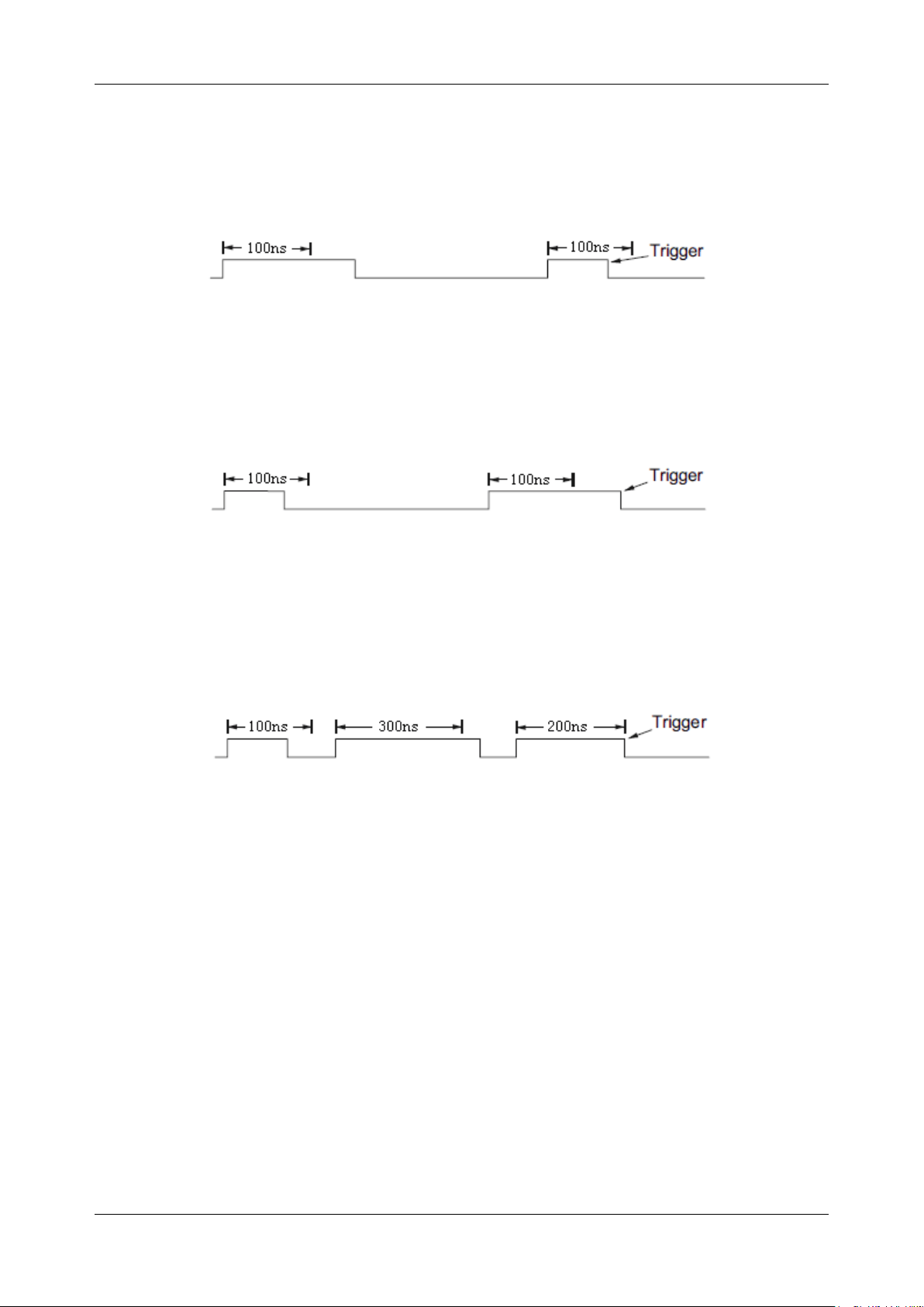
SDS6000L User Manual
int. s i g l e n t . c o m 93
Less than a time value
(
≤
)
-- Trigger when the positive or negative pulse time of the input signal is
lower than the specified time value. Below is an example of a trigger condition set to a positive pulse
width < 100ns
Great than a time value
(≥)-- Trigger when the positive or negative pulse time of the input signal is
greater than the specified time value. Below is an example of a trigger condition set to a positive pulse
width > 100ns
Within a range of time values
(
[--,--]
)
-- Trigger when the positive or negative pulse time of the input
signal is greater than the specified lower limit of time and lower than the specified upper limit of the
time value. Below is an example of a trigger condition set to 100 ns < positive pulse width < 300 ns.
Outside a range of time value
(
--][--
)
-- trigger when the positive or negative pulse time of the input
signal is greater than the specified upper limit of time and lower than the specified lower limit of the
time value.
Holdoff, coupling, and noise reject can be set in pulse trigger, see the sections "Holdoff", "Trigger
Coupling" and "Noise Reject" for details.
SDS6000L User Manual
94 i n t . s i g l e n t . c o m
13.5.5 Video Trigger
Video trigger can be used to capture the complicated waveforms of most standard analog video signals.
The trigger circuitry detects the vertical and horizontal interval of the waveform and produces a trigger
based on the video trigger settings you have selected. The SDS6000L supports standard video signals
for NTSC (National Television Standards Committee), PAL (Phase Alternating Line), HDTV (High-
Definition Television), and a custom video signal trigger.
Source, standard, and synchronization mode can be set in the video trigger dialog box. When the
synchronization mode is "Select", line and field can be specified.
Click the Standard and select the video standard. The SDS6000L supports the following video
standards:
TV Standard
Scan Type
Sync Pulse
NTSC
Interlaced
Bi-level
PAL
Interlaced
Bi-level
HDTV 720P/50
Progressive
Tri-level
HDTV 720P/60
Progressive
Tri-level
HDTV 1080P/50
Progressive
Tri-level
HDTV 1080P/60
Progressive
Tri-level
HDTV 1080i/50
Interlaced
Tri-level
HDTV 1080i/60
Interlaced
Tri-level
Custom
SDS6000L User Manual
int. s i g l e n t . c o m 95
The table below shows the parameters of the custom video trigger:
Frame Rate
25Hz, 30 Hz, 50 Hz,60 Hz
Of Lines
300 ~ 2000
Of Fields
1,2,4,8
Interlace
1:1, 2:1,4:1,8:1
Trigger Position
Line
Field
(line value)/1(1:1)
1
(line value)/2 (2:1)
1,2, 3, 4,5,6,7,8
(line value)/4(4:1)
1,2, 3, 4,5,6,7,8
(line value)/8(8:1)
1,2, 3, 4,5,6,7,8
Line value: The number of lines set in the Of Lines (300 ~ 2000).
In the custom video trigger type, the corresponding "Of Fields" varies with the selection of the “Interlace”
ratio. Therefore, the number of fields selected and the number of lines corresponding to each field can
also be varied. If the "Of Lines" is set to 800, the correct relationship between them is as follows:
Of Lines
Interlace
Of Fields
Trigger Line
Trigger Field
800
1:1
1
800
1
800
2:1
1/2/4/8
400
1/1~2/1~4/1~8
800
4:1
1/2/4/8
200
1/1~2/1~4/1~8
800
8:1
1/2/4/8
100
1/1~2/1~4/1~8
Set the video trigger for a video signal
Click Sync for trigger mode selection, video trigger mode has "Any" and "Select" options. In "Any"
mode, the video signal can be triggered on any line that meets the conditions. In the "Select" mode,
the signal can be triggered by a specified field and a specified line.

SDS6000L User Manual
96 i n t . s i g l e n t . c o m
For progressive scanning signals (e.g. 720p/50, 720p/60, 1080p/50, 1080p/60), only the specified line
can be selected to trigger when the synchronization mode is “Select”.
For interlaced scanning signals (such as NTSC, PAL, 1080i/50, 1080i/60, and Custom), when the
synchronization mode is "Select", the specified line and the specified field can be selected to trigger.
The following table shows the corresponding relations between line and field for all video standards
(except for Custom)
Standard
Field 1
Field 2
NTSC
1 to 263
1 to 262
PAL
1 to 313
1 to 312
HDTV 720P/50 , 720P/60
1 to 750
HDTV 1080P/50 , 1080P/60
1 to 1125
HDTV 1080i/50 , 1080i/60
1 to 563
1 to 562
To gain familiarization with the video trigger, try these two examples:
Trigger on a specific line of video (NTSC standard)
Use “Custom” to trigger video signals
Trigger on a Specific Line of Video
Video trigger requires that any analog channel can be used as the trigger source with a synchronization
amplitude greater than 1/2 grid. The example below sets to trigger on Field 1, Line 22 using the NTSC
video standard.
1. Open the trigger menu.
2. In the trigger menu, click Type , and select "Video".
3. Click the Source and select CH1 as the trigger source.
4. Click the Standard and select the "NTSC".
5. Click the Sync and select the "Select" to make the Field and Line optional, then select "1"
in the "Field", and set the "Line" to "22" by using the mouse wheel or the virtual keypad.
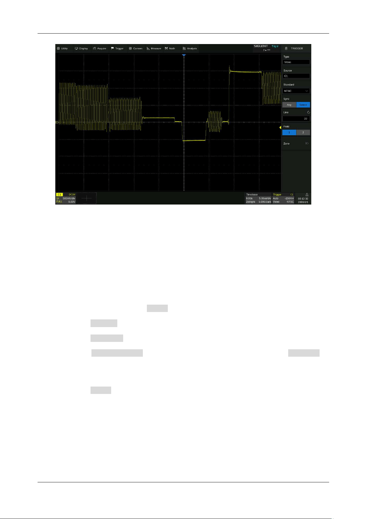
SDS6000L User Manual
int. s i g l e n t . c o m 97
Trigger on a Specific Line of Video (NTSC)
Use "Custom" to Trigger Video Signals
Custom video trigger supports video signals with frame rates of 25, 30, 50, and 60 Hz respectively,
and the specified row is within the range of 300 to 2000. The following describes how to trigger a
"Custom" video signal.
1. Open the trigger menu.
2. In the trigger menu, click the Type , and select "Video".
3. Click the Source and select CH1 as the trigger source.
4. Click the Standard and select the "Custom".
5. Click the Custom Setting to open the custom setting menu and click the Interlace to
select the required interlace ratio (assuming that the interlace ratio is 8:1). Then set the frame
rate and select the number of lines and the number of fields.
6. Click the Sync to select the synchronization mode for the input signal:
a) Select the "Any" mode, and the signal can be triggered on any line that meets the trigger
condition.
b) Select the "Select" mode, then set the specified line and the specified field to trigger the
signal. Assuming that the "Field" is set to 8, you can select any field from 1 to 8, and
each field can choose any line from 1 to 100.
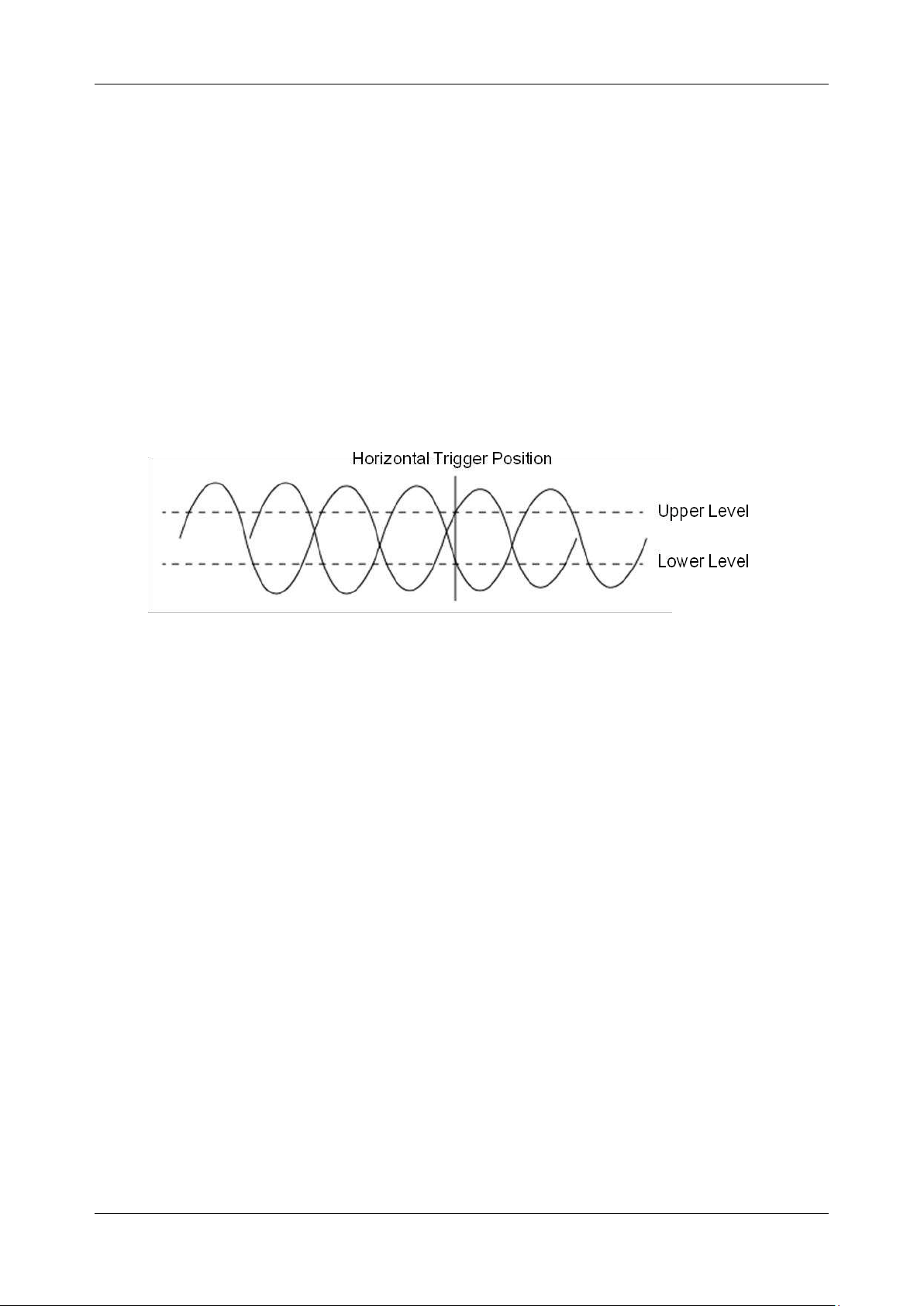
SDS6000L User Manual
98 i n t . s i g l e n t . c o m
13.5.6 Window Trigger
The window trigger is similar to the edge trigger, except that it provides an upper and a lower trigger
level. The instrument triggers when the input signal passes through the upper level or the lower level.
There are two kinds of window types: Absolute and Relative. They have different trigger-level
adjustment methods. Under the Absolute window type, the lower and the upper trigger levels can be
adjusted separately. The relative window provides adjustment for the Center value to set the window
center and the Delta value to set the window range. In this mode, the lower and the upper trigger levels
always move together.
If the lower and the upper trigger levels are both within the waveform amplitude range, the
oscilloscope will trigger on both rising and falling edges.
If the upper trigger level is within the waveform amplitude range while the lower trigger level
is out of the waveform amplitude range, the oscilloscope will trigger on the rising edge only.
If the lower trigger level is within the waveform amplitude range while the upper trigger level
is out of the waveform amplitude range, the oscilloscope will trigger on the falling edge only.
To set window trigger via the Absolute window type
Refer to "Adjust Upper/Lower Level" in the section "Slope Trigger".
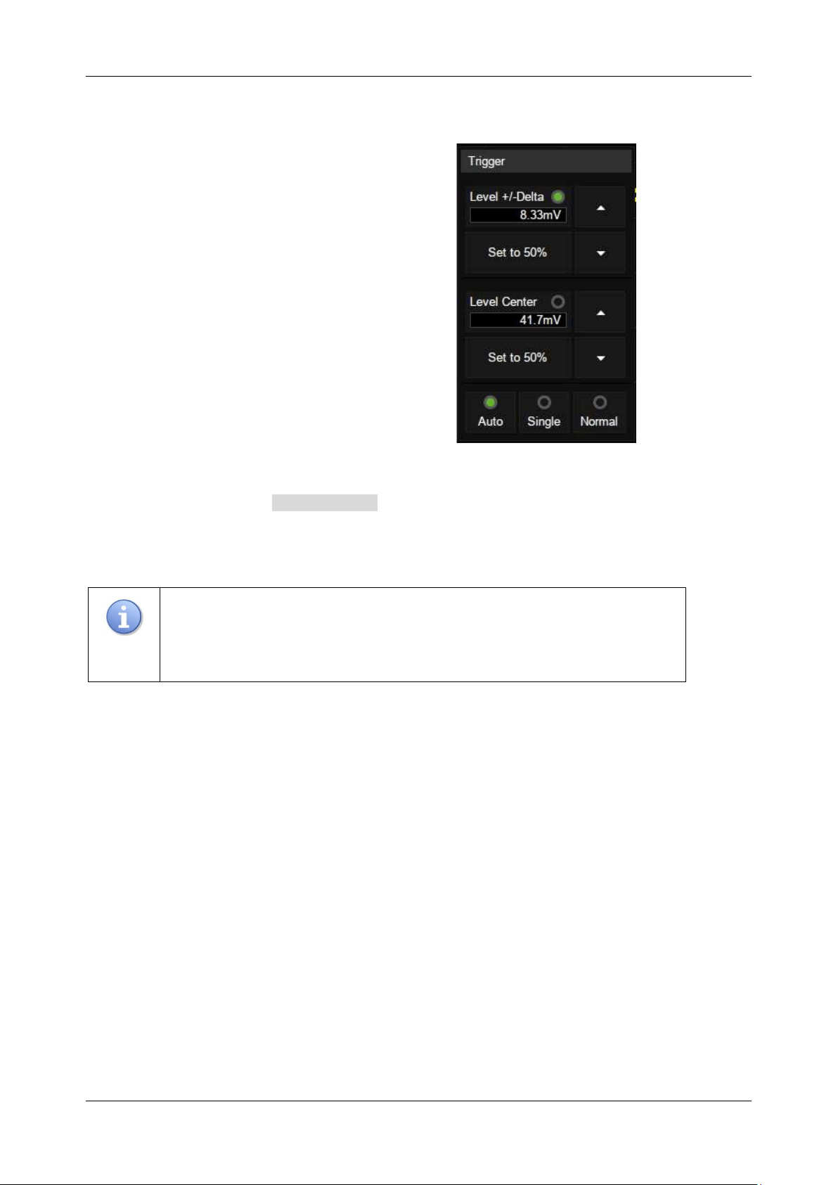
SDS6000L User Manual
int. s i g l e n t . c o m 99
To set window trigger via the Relative window type
When the window trigger type is set to "Relative",
click the trigger descriptor box. The pop-up
menu will show two user-defined parameters:
“Level +/-Delta" and "Level Center".
The above two parameters can be set in the
following way:
Select the parameter in the Level +/-Delta area of the quick menu, then set the parameter value by
the virtual keypad or the mouse wheel. Setting the center level is similar.
Note:
"Level +/-Delta” represents half of the actual window area. For example,
when the value is 200mV, it represents a range of ±200 mV, which is a 400mV
window.
Holdoff, coupling, and noise reject can be set in the window trigger, see the sections "Holdoff", "Trigger
Coupling" and "Noise Reject" for details.
13.5.7 Interval Trigger
Trigger when the time difference between the neighboring rising or falling edges meets the time limit
condition.
When the trigger condition is set as an interval between two neighboring rising edges and it is less than
the set time value, the trigger diagram is as follows:
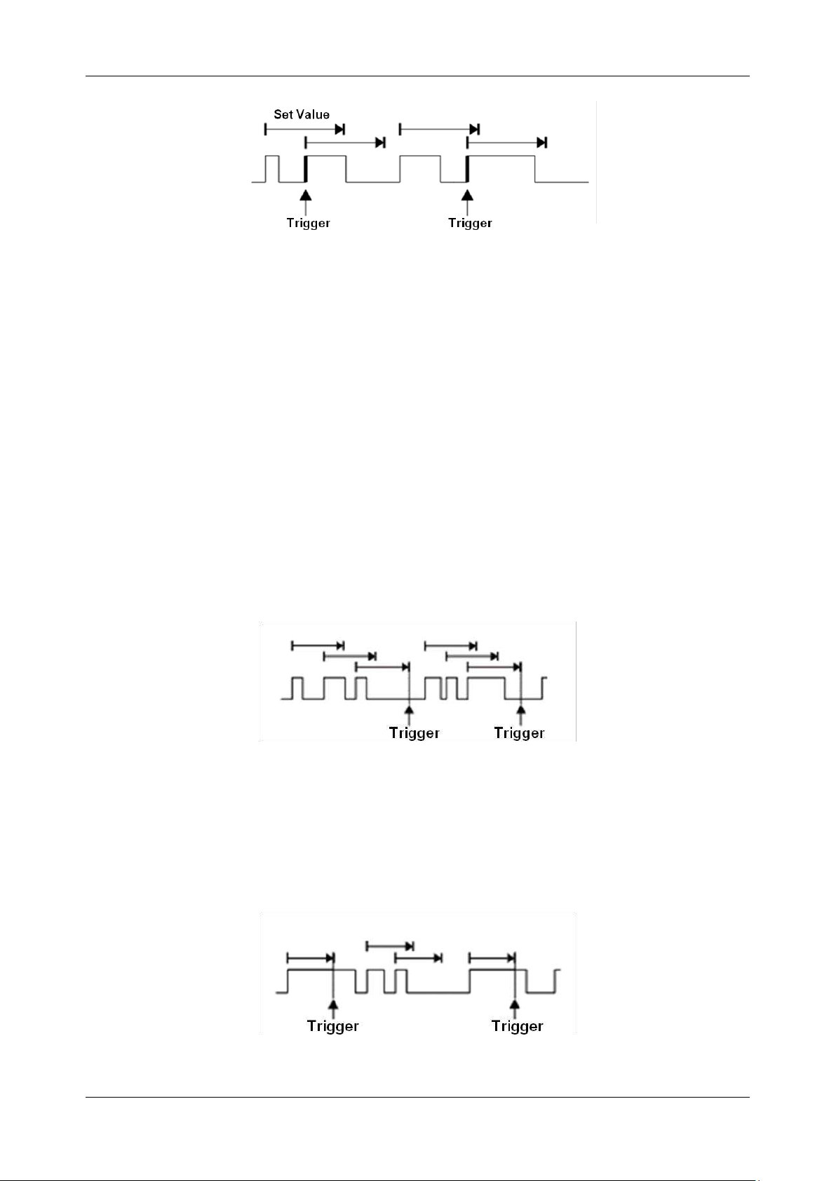
SDS6000L User Manual
1 0 0 i n t . s i g l e n t . c o m
Trigger source, slope (rising, falling), limit range, and time value can be set in the trigger dialog box.
Holdoff, coupling, and noise reject can be set in interval trigger, see the sections "Holdoff", "Trigger
Coupling" and "Noise Reject" for details.
13.5.8 Dropout Trigger
Dropout trigger includes two types: Edge and State.
Edge
Trigger when the time interval (
△
T) from when the rising edge (or falling edge) of the input signal
passes through the trigger level to when the neighboring rising edge (or falling edge) passes through
the trigger level is greater than the set time, as shown in the figure below:
State
Trigger when the time interval (
△
T) from when the rising edge (or falling edge) of the input signal
passes through the trigger level to when the neighboring falling edge (or rising edge) passes through
the trigger level is greater than the set time, as shown in the figure below:
Trigger source, slope (rising, falling), dropout type, and time value can be set in the trigger dialog box.
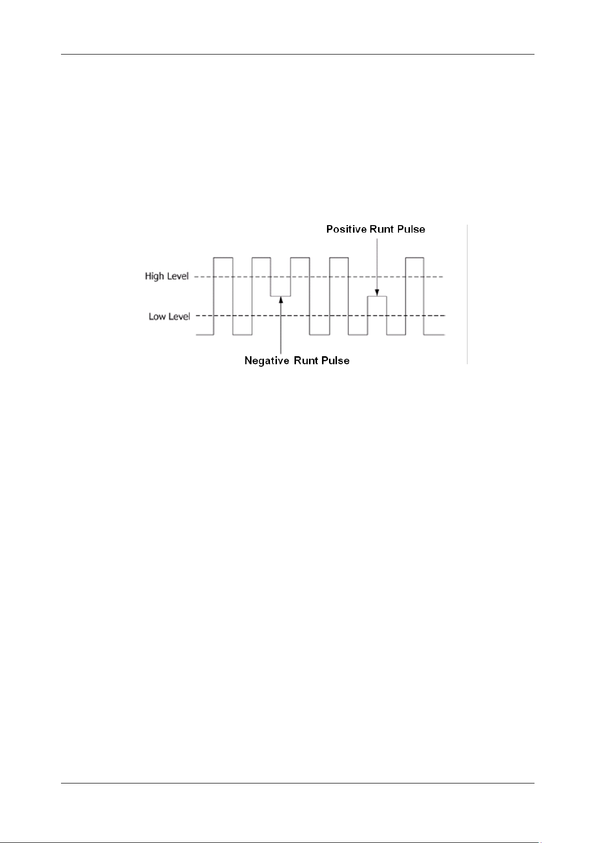
SDS6000L User Manual
int. s i g l e n t . c o m 1 0 1
Holdoff, coupling, and noise reject can be set in the dropout trigger, see the sections "Holdoff", "Trigger
Coupling" and "Noise Reject" for details.
13.5.9 Runt Trigger
Runt trigger looks for pulses that cross one threshold but not another as shown in the figure below:
A positive runt pulse across through the low level but not the high level.
A negative runt pulse across through the high level but not the low level.
Holdoff, coupling, and noise reject can be set in the dropout trigger, see the sections "Holdoff", "Trigger
Coupling" and "Noise Reject" for details.
13.5.10 Pattern Trigger
The Pattern trigger identifies a trigger condition by looking for a specified pattern. The SDS6000L
provides 4 patterns: logical AND, OR, NAND and NOR combination of the channels. Each channel can
be set to "Low", "High" or "Don't Care". If all channels are set to "Don’t Care", the oscilloscope will not
trigger. The result after the logical operation is triggered from true to false, that is, triggers on the falling
edge of the combined waveform.
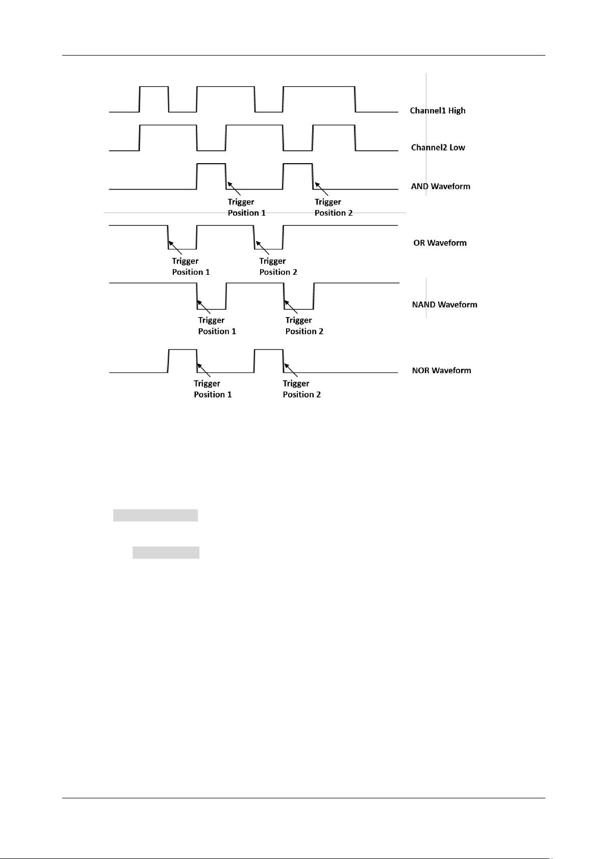
SDS6000L User Manual
1 0 2 i n t . s i g l e n t . c o m
Logic (AND, OR, NAND, NOR), source, limit range, and time value can be set in the trigger dialog box.
Source Setting
Click the Source Setting area to recall the following dialog box and set up for each channel
separately. Each channel can be set to "Low", "High" or "Don't Care". The threshold can be determined
by setting the Level Value .
When digital channels are turned on, the logic state of the digital channel can also be set in the source
setting dialog box.
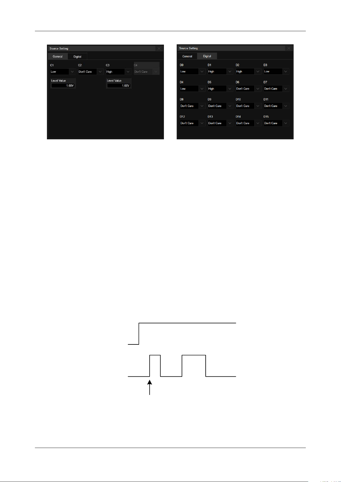
SDS6000L User Manual
int. s i g l e n t . c o m 1 0 3
The logical setting of analog channels
The logical setting of digital channels
Limit Range
This setting is particularly useful to filter the hazard signals of combinational logic.
Holdoff can be set in pattern trigger, see the section "Holdoff" for details.
13.5.11 Qualified Trigger
The qualified trigger is an edge trigger after a user-defined qualified condition is satisfied. So a qualified
trigger has two sources; one is the source of the edge trigger, and the other is the qualified source.
The qualified types include “State”, “State with Delay”, “Edge”, and “Edge with Delay”. When the type
is “State”, the oscilloscope triggers on the first edge when the qualified source is in the specified state
(High or Low). When the type is “State with Delay”, a time limit condition is also available.
Qualified
Source
Edge
Trigger
Source
Trigger
Position
Qualified State = High
Edge = Rising
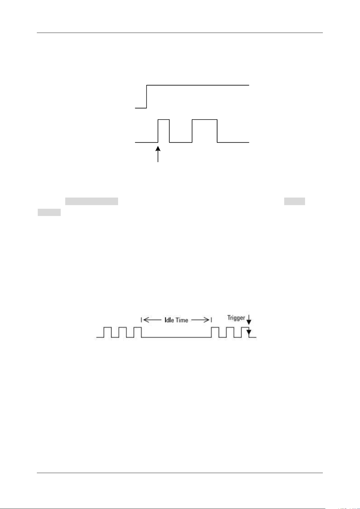
SDS6000L User Manual
1 0 4 i n t . s i g l e n t . c o m
When the type is “Edge”, the oscilloscope triggers at the first edge after the specified edge (Rising or
Falling) of the qualified source; when the type is “Edge with Delay”, a time limit condition is available.
Qualified
Source
Edge
Trigger
Source
Trigger
Position
Qualified Edge = Rising
Edge = Rising
Click the Qualified Setting region to set the qualified source and threshold; Click the Edge
Setting region to set the edge trigger source, threshold, and slope.
13.5.12 Nth Edge Trigger
Nth edge trigger is similar to an edge trigger with conditions. The trigger is satisfied after meeting the
user-defined idle time and edge number conditions. As shown in the figure below, when the idle time
between the pulse trains is greater than the specified idle time, it is triggered on the third falling edge
of the pulse train.
Trigger source, slope (rising, falling), idle time, and edge number can be set in the trigger dialog box.
Holdoff, coupling, and noise reject can be set in the Nth edge trigger, see the sections "Holdoff",
"Trigger Coupling" and "Noise Reject" for details.
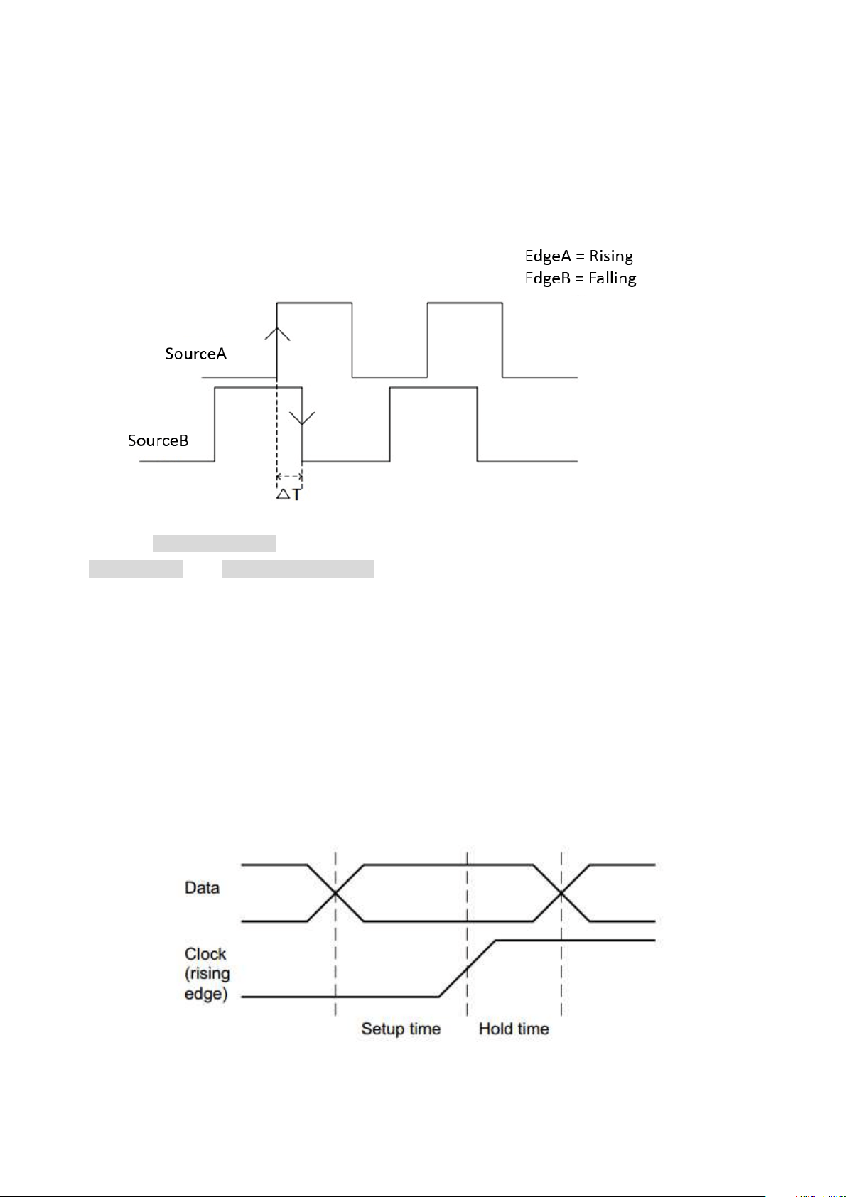
SDS6000L User Manual
int. s i g l e n t . c o m 1 0 5
13.5.13 Delay Trigger
A delay trigger is true when the edge of source B occurs after meeting the set conditions of source A
and a user-defined delay time. The setting of source A is similar to that of the pattern trigger and can
be used for logical "and" combination of multiple channels.
Click the SourceB Setting region to set the edge trigger source, threshold, and slope. Click the
Limit Range and Upper / Lower Value region to set the delay time condition.
13.5.14 Setup/Hold Trigger
The clock and data sources need to be set in the setup/hold trigger setting. The set-up time starts when
the data signal crosses the trigger level and ends when the specified clock edge arrives. The holding
time starts when the specified clock edge arrives and ends when the data signal crosses the trigger
level again (as shown in the figure below). When the set-up time or hold time meets the preset time
limit conditions, the oscilloscope will trigger.

SDS6000L User Manual
1 0 6 i n t . s i g l e n t . c o m
Click the CLK Setting region to set the clock source, threshold, and slope; Click the Data Setting
region to set the data source, threshold, and state.
13.5.15 Serial Trigger
Refer to Chapter “Serial Trigger and Decode” for detailed information.
13.6 Trigger Source
The trigger sources supported by each trigger type are different. See the table below for details:
Trigger Type
C1~C8
EXT, EXT/5
AC Line
D0~D15
Edge
√
√
√
√
Slope
√
×
×
×
Pulse
√
×
×
√
Video
√
×
×
×
Window
√
×
×
×
Interval
√
×
×
√
Dropout
√
×
×
√
Runt
√
×
×
×
Pattern
√
×
×
√
Serial
√
×
×
√
Qualified
√
×
×
√
Nth Edge
√
×
×
√
Delay
√
×
×
√
Setup/Hold
√
×
×
√
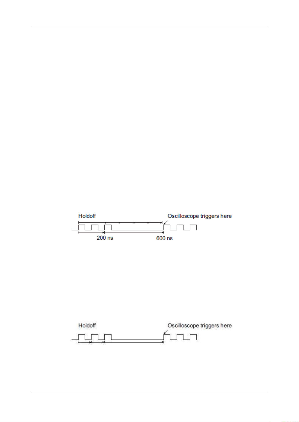
SDS6000L User Manual
int. s i g l e n t . c o m 1 0 7
13.7 Holdoff
Holdoff is an additional condition for triggers and can be used to stabilize the triggering of complex
waveforms (such as a pulse series). It can be set to a time or number of events.
Holdoff by Time
Holdoff time is the amount of time that the oscilloscope waits before re-arming the trigger circuitry. The
oscilloscope will not trigger until the holdoff time expires.
Use the holdoff to trigger on repetitive waveforms that have multiple edges (or other events) between
waveform repetitions. You can also use holdoff to trigger on the first edge of a burst when you know
the minimum time between bursts.
For example, to achieve a stable trigger on the repetitive pulses shown in the figure below set the
holdoff time (t) to 200ns<t<600ns.
Holdoff by Event
The Holdoff event sets the number of events that the oscilloscope counts before re-arming the trigger
circuitry. The oscilloscope will not trigger until the counter that tracks holdoff events reaches the set
value. In the following figure, the holdoff event is set to 3, and the signal is triggered on the fourth edge.
Parameter
Start Holdoff On
defines the initial position of holdoff.

SDS6000L User Manual
1 0 8 i n t . s i g l e n t . c o m
Acq Start
-- The initial position of holdoff is the first-time point satisfying the trigger condition. In the
example above, each holdoff starts from the first rising edge of the pulse sequence.
Last Trig Time
--The initial position of holdoff is the time of the last trigger. In the example above, the
last trigger position is at the second rising edge of the pulse sequence and the second holdoff starts
from that point.
13.8 Trigger Coupling
The coupling setting of a trigger is only valid when the trigger source is C1~C8, EXT, or EXT/5.
DC: All of the signal’s frequency components are coupled to the trigger circuit for high-frequency
bursts or where the use of AC coupling would shift the effective trigger level.
AC: The signal is capacitively coupled. DC levels are rejected. See the datasheet for details of the
cut-off frequency.
HFR: Signals are DC coupled to the trigger circuit and a low-pass filter network attenuates high
frequencies (used for triggering on low frequencies). See the datasheet for details of the cut-off
frequency.
LFR: The signal is coupled through a capacitive high-pass filter network, DC is rejected and low
frequencies are attenuated. For stable triggering on medium to high-frequency signals. See the
datasheet for details of the cut-off frequency.
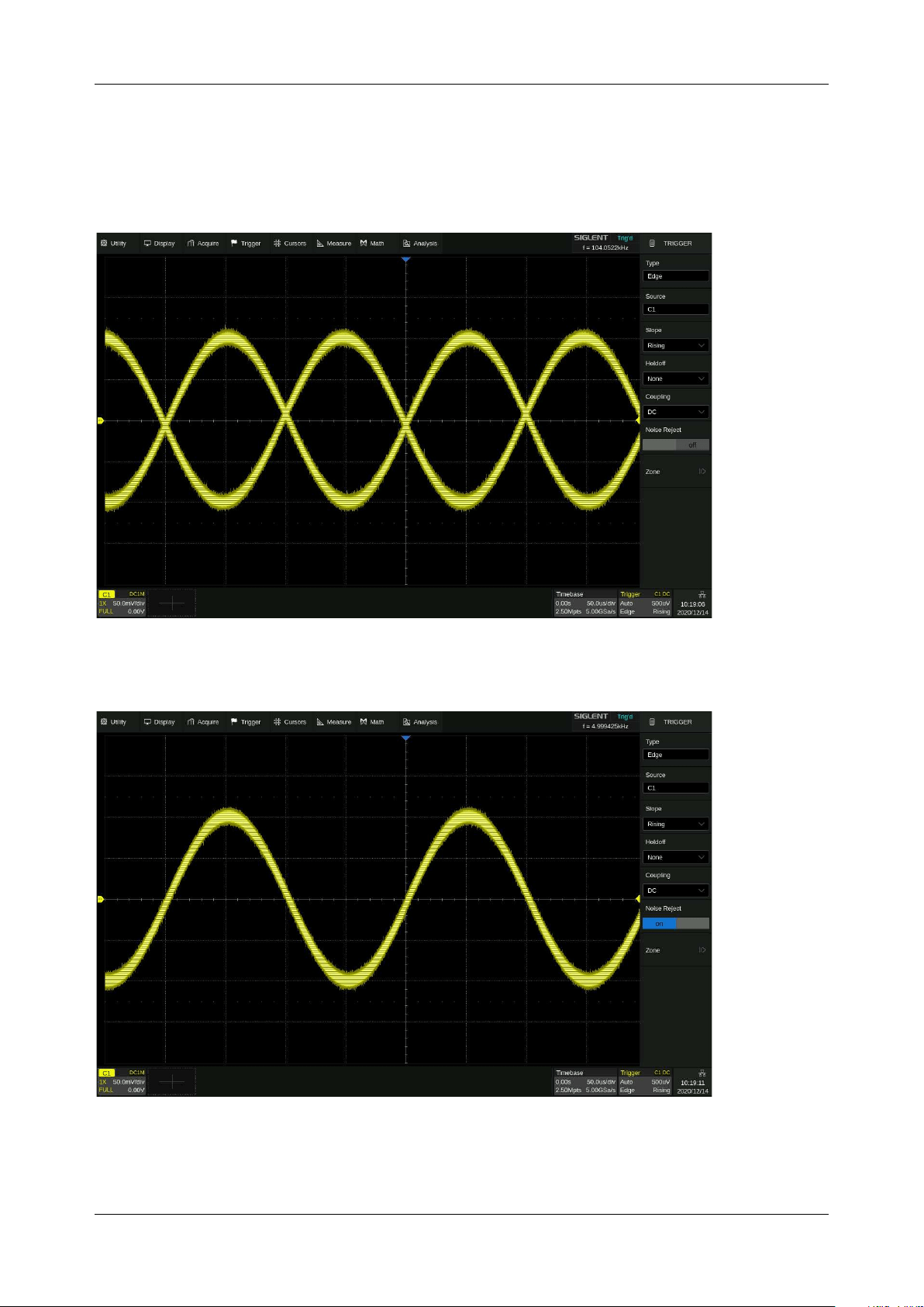
SDS6000L User Manual
int. s i g l e n t . c o m 1 0 9
13.9 Noise Reject
Noise Reject adds additional hysteresis to the trigger circuitry. By increasing the trigger hysteresis, the
noise immunity becomes better but the trigger sensitivity degrades.
Noise Reject = Off
Noise Reject = On
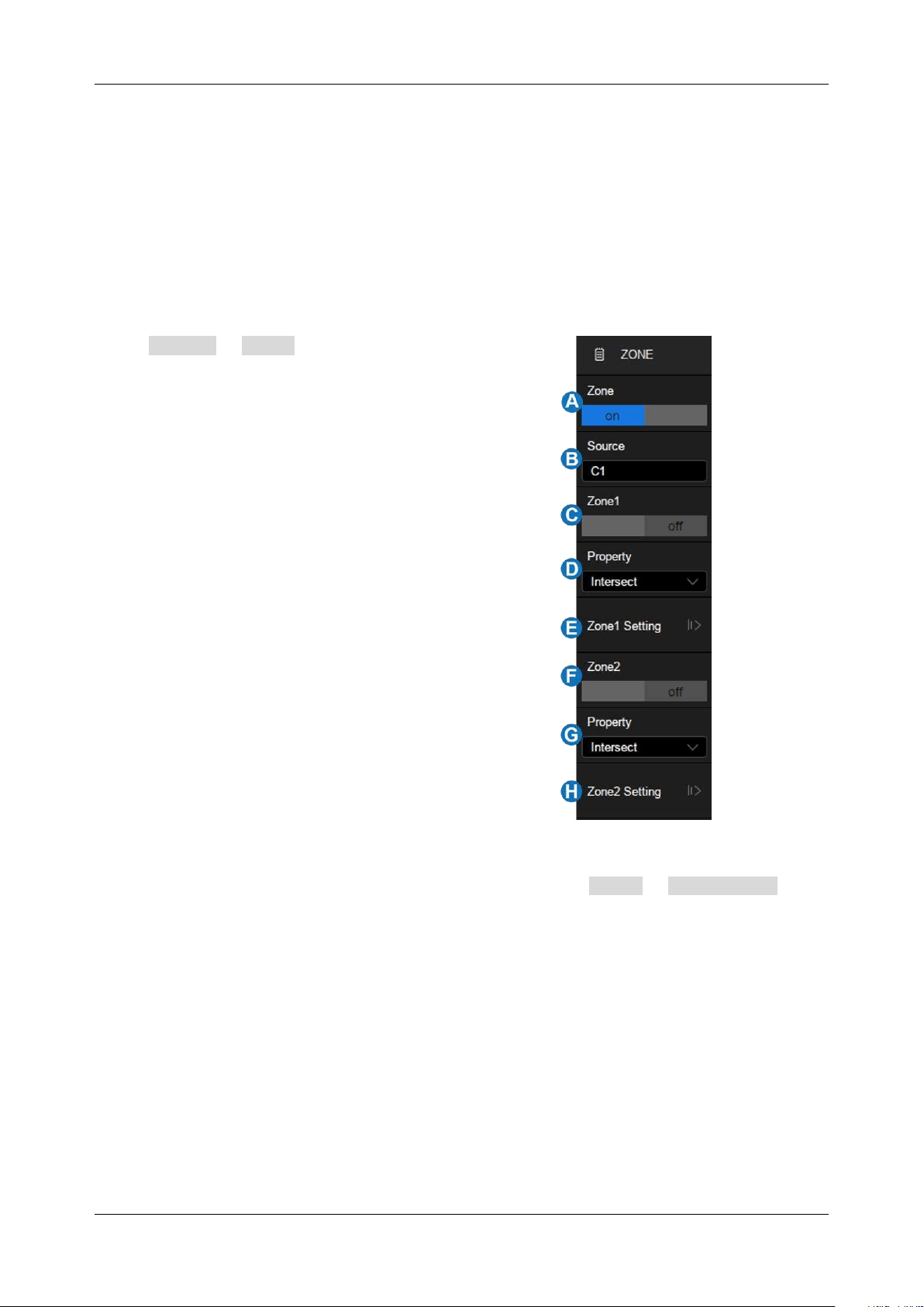
SDS6000L User Manual
11 0 i n t . s i g l e n t . c o m
13.10 Zone Trigger
The SDS6000L includes a zone trigger to help isolate elusive glitches. There are two user-defined
areas: Zone1 and Zone2. Users can set the property of each zone as “intersect” or “not intersect” as
an additional condition to further isolate the interesting event quickly. “Intersect” only includes events
that occur within the zone. “Not-intersect” events include all events that occur outside of the zone.
Click Trigger > Zone to recall zone dialog box:
A. Turn on or off zone trigger
B. Select the source: C1~C8
C. Turn on or off zone1
D. Set the property of zone1: Intersect or Not
intersect
E. Set the coordinate of zone1. The range is
within the waveform area
F. Turn on or off zone2
G. Set the property of zone2: Intersect or Not
intersect
H. Set the coordinate of zone2. The range is
within the waveform area
The zones can be created and moved by the mouse or by setting Zone > Zone Setting in the
dialog box. The color of the zone’s outline is consistent with the color of the specified source (Channel
1 = Yellow, etc...).
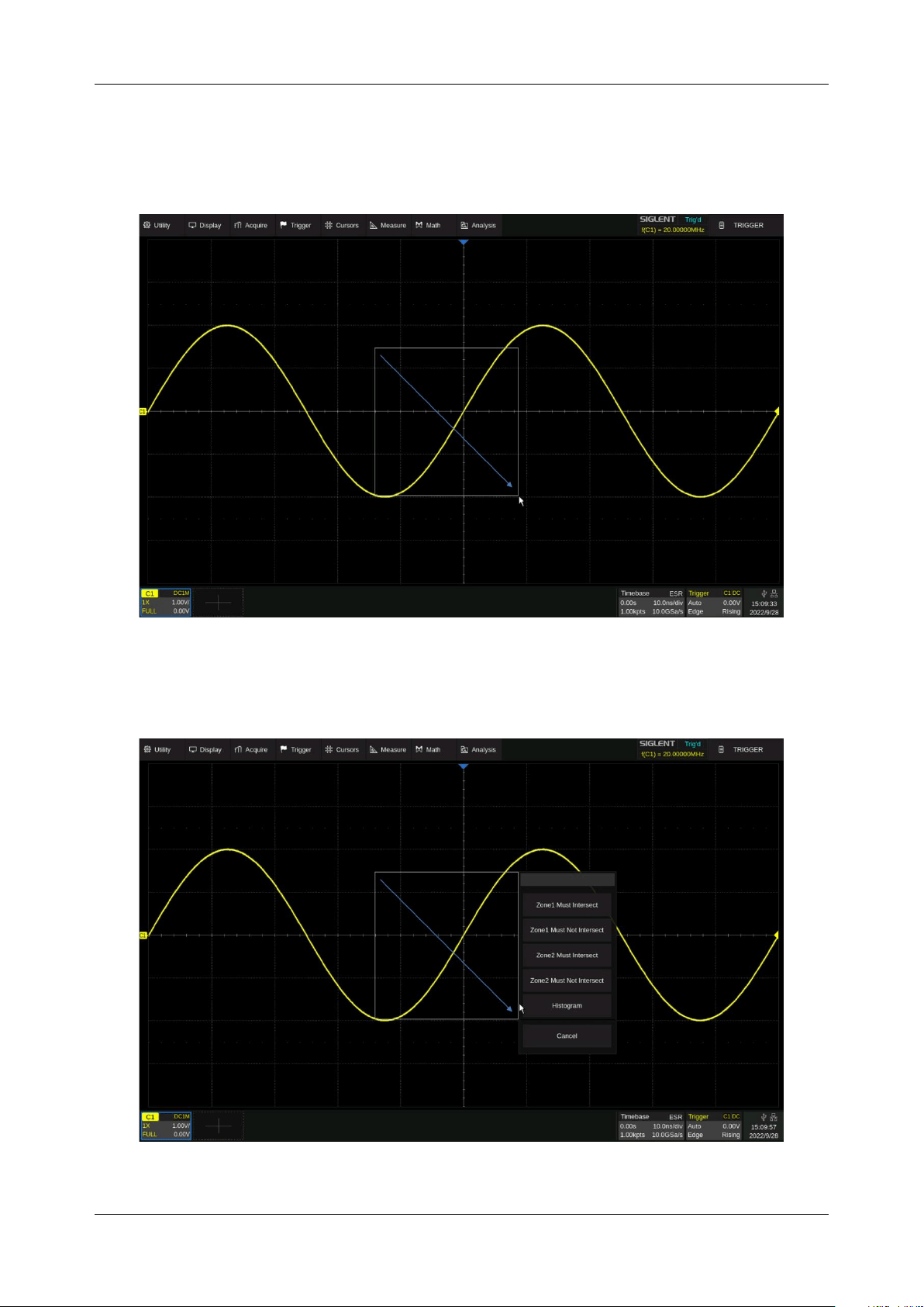
SDS6000L User Manual
int. s i g l e n t . c o m 111
Mouse
When the zone trigger is turned on, click-and-hold on any position within the waveform area and draw
a rectangular box, as shown in the following figure:
When the finger moves out of the screen, a menu pops up for selecting the zone and setting the zone
properties:
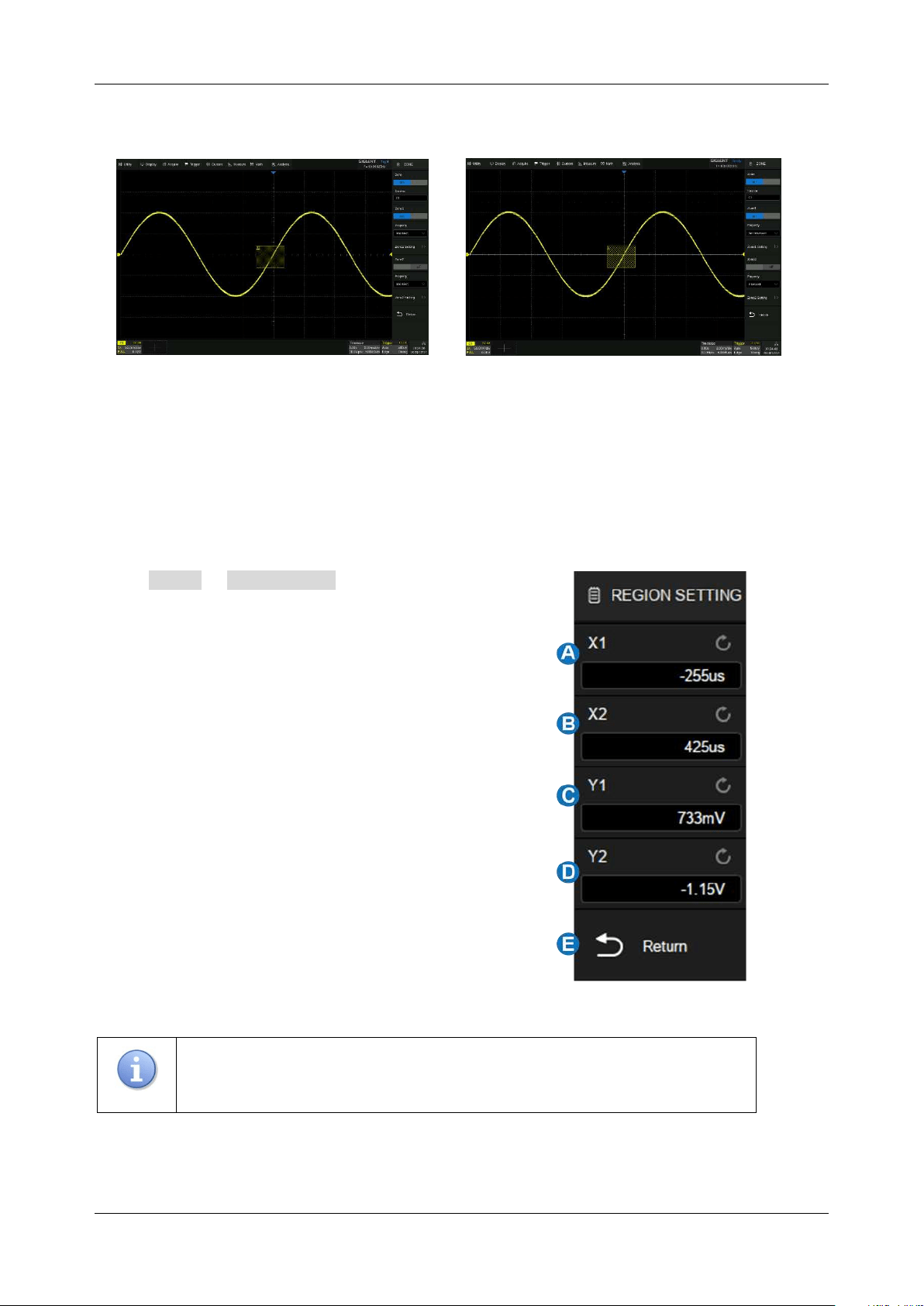
SDS6000L User Manual
11 2 i n t . s i g l e n t . c o m
Once a zone is created, it can be moved by dragging.
Select C1 as the source, turn on zone1,
and set the property as "Intersect"
Select C1 as the source, turn on zone1,
and set the property as "Not Intersect"
Dialog Box
Click Zone > Zone Setting to recall the dialog box.
A. Set the left border of the zone
B. Set the right border of the zone
C. Set the top border of the zone
D. Set the bottom border of the zone
E. Return to the previous menu
Click the regions above to set the value by the mouse
wheel or the virtual keypad.
Note:
If zone1 and zone2 are both turned on, the result of the "AND" operation
in two zones becomes the qualified condition of triggering.
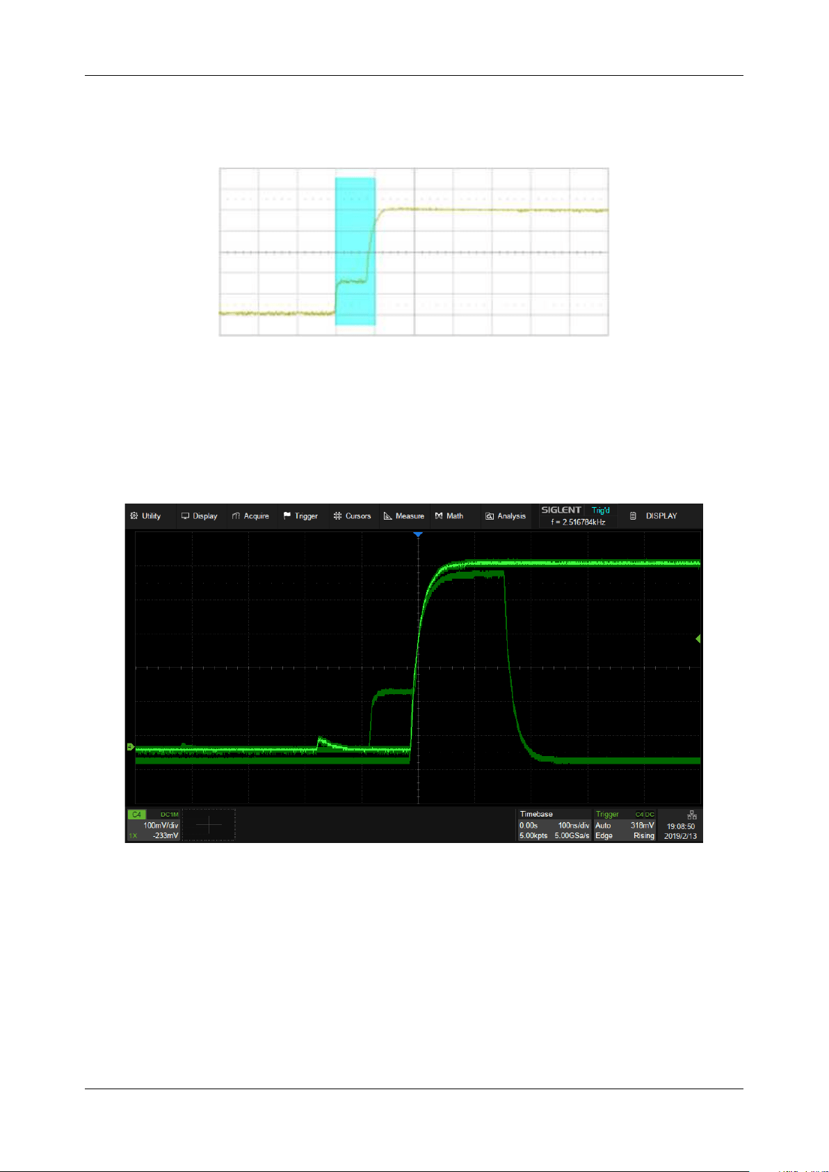
SDS6000L User Manual
int. s i g l e n t . c o m 11 3
Below is an example in which we want to capture a waveform of bus contention using the SDS6000L:
With a simple edge trigger, it is unlikely to trigger consistently on this anomaly. Thanks to the high
waveform update rate of the SDS6000L, we can confirm there is bus contention happening by enabling
the persistence display, as shown in the figure below:
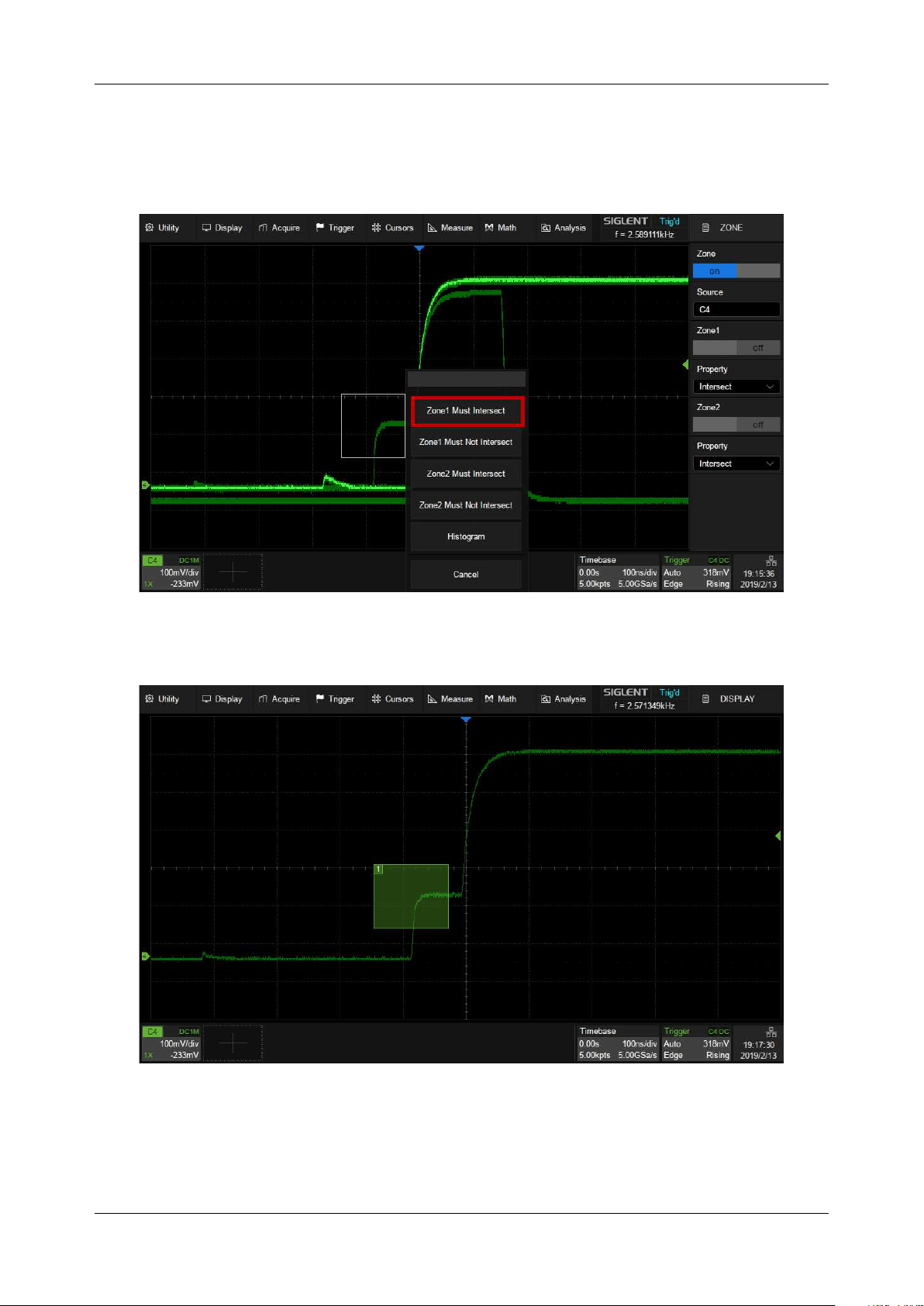
SDS6000L User Manual
11 4 i n t . s i g l e n t . c o m
In this case zone trigger is a quick and simple way to capture the waveform. Enable the zone trigger,
and draw a box to intersect with the bus contention part, as shown in the figure below:
Now, we can accurately capture the exact bus contention waveform:
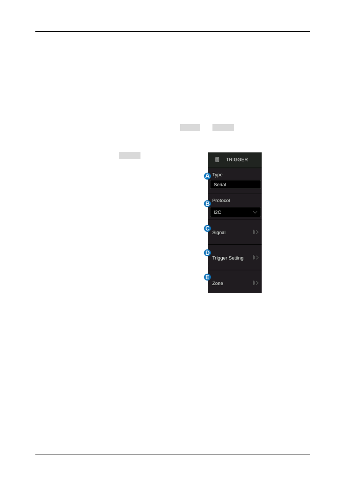
SDS6000L User Manual
int. s i g l e n t . c o m 11 5
14 Serial Trigger and Decode
14.1 Overview
The SDS6000L supports serial bus trigger and decode on the following serial bus protocols: I2C, SPI,
UART, CAN, LIN, FlexRay, CAN FD, I2S, MIL-STD-1553B, SENT, and Manchester.
Click the trigger descriptor box, and then select the Type as Serial in the trigger dialog box to
set the serial trigger:
A. Select the type as Serial
B. Select the serial bus protocol
C. Set the signal, including the mapping
relation between channels and bus
signals, and the thresholds
D. Trigger setting
E. Zone setting
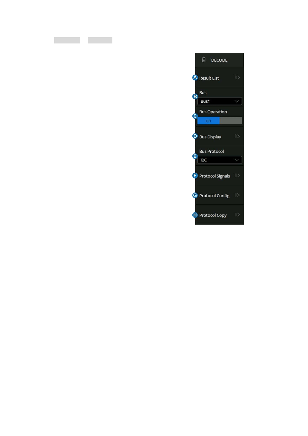
SDS6000L User Manual
11 6 i n t . s i g l e n t . c o m
Perform Analysis > Decode to turn on the serial decode dialog box:
A. Set the list of decoded results
B. Select the bus to set, Bus1 and Bus2
C. Turn on/off the bus
D. Set the bus display format (Binary, Decimal,
Hex, and ASCII)
E. Select the serial bus protocol
F. Click to set the signal, including the mapping
relation between channels and bus signals,
and the thresholds. This is similar to the signal
setting of a serial trigger.
G. Configure the bus protocol
H. Synchronize the settings between a serial
trigger and decode
Below are detailed descriptions of the trigger and decode steps for each protocol.
I2C Trigger and Serial Decode
SPI Trigger and Serial Decode
UART Trigger and Serial Decode
CAN Trigger and Serial Decode
LIN Trigger and Serial Decode
FlexRay Trigger and Serial Decode
CAN FD Trigger and Serial Decode
I2S Trigger and Serial Decode
MIL-STD-1553B Trigger and Serial Decode
SENT Trigger and Serial Decode
Manchester Serial Decode
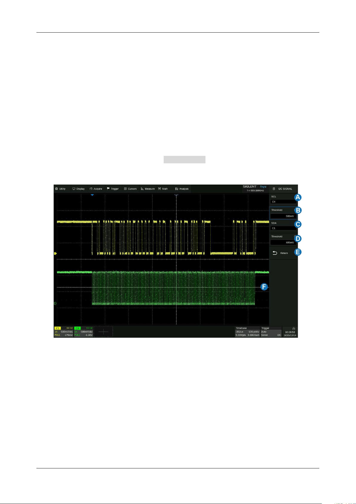
SDS6000L User Manual
int. s i g l e n t . c o m 11 7
14.2 I2C Trigger and Serial Decode
This section covers triggering and decoding I2C signals. Please read the following for more details:
"I2C Signal Settings", "I2C Trigger" and "I2C Serial Decode".
14.2.1 I2C Signal Settings
Connect the serial data signal (SDA) and the serial clock signal (SCL) to the oscilloscope, set the
mapping relation between channels and signals, and then set the threshold level of each signal. The
signal settings of the decode and trigger are independent. If you want to synchronize the settings
between decode and trigger, please perform Copy Setting in the decode dialog box.
A. Set the source of SCL. In the example above, SCL is connected to C4.
B. Set the threshold level of SCL. It is 1.7V for the LVTTL signal in this example.
C. Set the source of SDA. In the example above, SDA is connected to C1.
D. Set the threshold level of the SDA channel.
E. Return to the previous menu.
F. Threshold level line. It only appears when adjusting the threshold level.
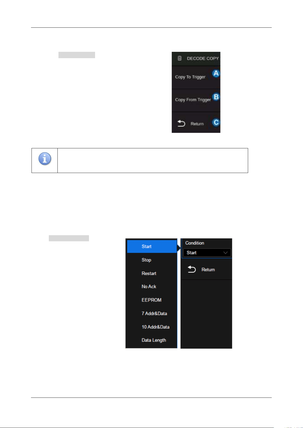
SDS6000L User Manual
11 8 i n t . s i g l e n t . c o m
Copy Setting
Click the Copy Setting in the decode dialog
box to synchronize the settings between the
trigger and decode.
A. Copy the decode settings to trigger
B. Copy the trigger settings to decode
C. Return to the previous menu.
Note:
The synchronization is not automatic. If the settings in one place
change, a copy operation is necessary to re-synchronize.
14.2.2 I2C Trigger
When the protocol is set to I2C, the following trigger conditions can be set: Start, Stop, Restart, No Ack,
EEPROM, or an R/W frame with a specific device address and data value.
Click Trigger Setting in the
I2C trigger dialog box to select
the trigger condition:
Start
-- The oscilloscope will be triggered when the SDA line transitions from high to low while the SCL
is high.
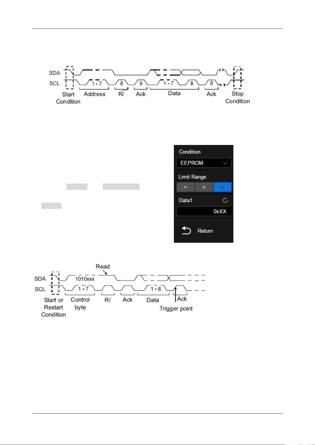
SDS6000L User Manual
int. s i g l e n t . c o m 11 9
Stop
-- The oscilloscope will be triggered when the SDA line transitions from low to high while the SCL
is high.
Restart
-- The oscilloscope will be triggered when another “Start” occurs before a “Stop".
No Ack
-- The oscilloscope will be triggered when the SDA line is high during any SCL’s ACK bit.
EEPROM
-- The trigger searches for EEPROM
control byte value 1010xxx on the SDA bus. And
there is a Read bit and an ACK bit behind
EEPROM. Set the data value and compare type
according to Data1 and Limit Range . If
EEPROM’s data is greater than (less than, equal
to) Data1 , the oscilloscope will be triggered
at the edge of the ACK bit behind the Data byte.
The Data byte doesn’t need to follow the
EEPROM.
7 Address & Data
-- the oscilloscope will be triggered on the read or write frame in 7-bit address mode.
Frame (Start: 7-bit address: R/W: Ack) -- Data1 and Data2 are set to “0xXX”. If all bits match, then
trigger on the Ack bit followed by the R/W bit.
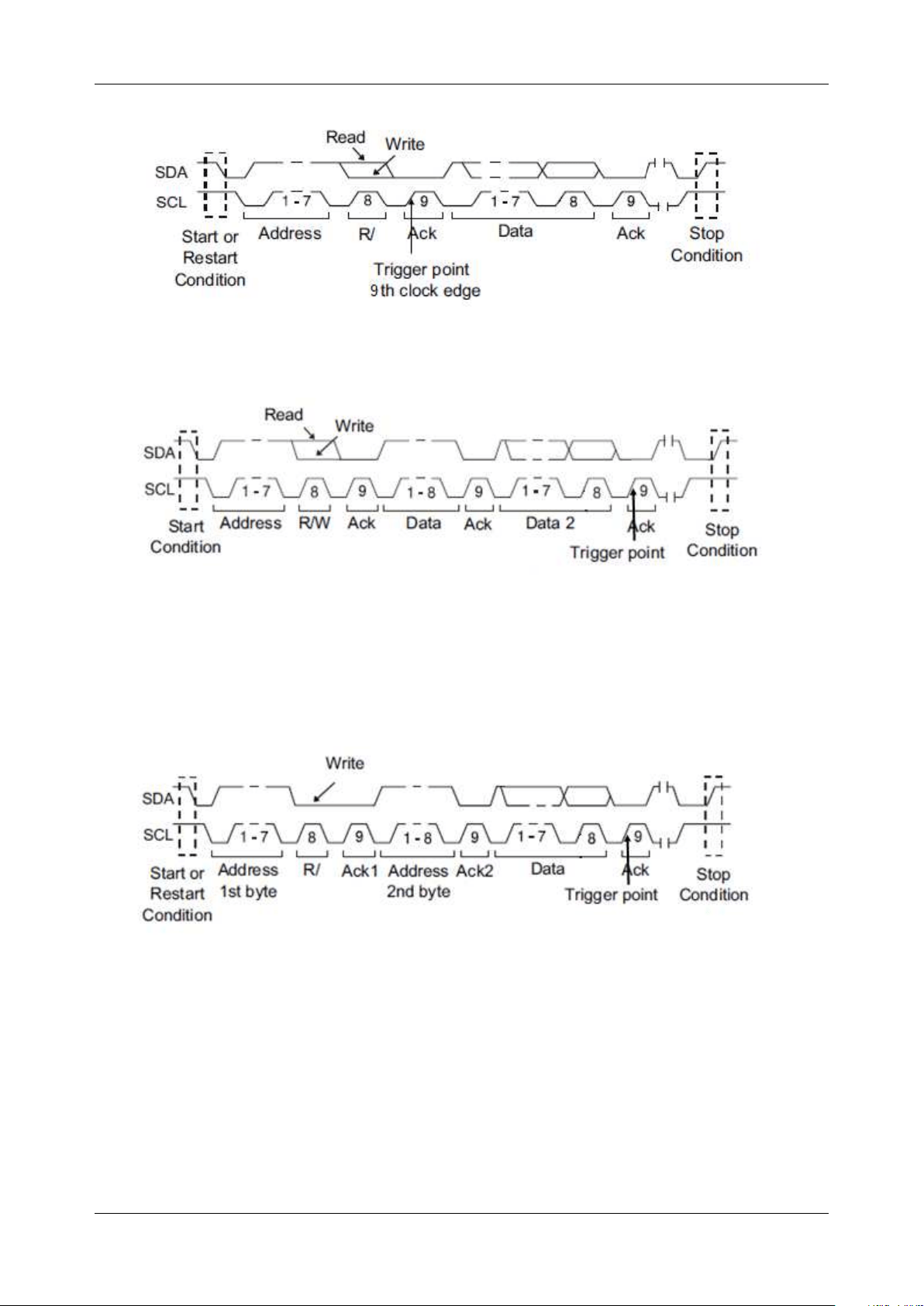
SDS6000L User Manual
1 2 0 i n t . s i g l e n t . c o m
Frame (Start: 7-bit address: R/W: Ack: Data: Ack: Data2) -- If all bits match, then trigger on the Ack bit
followed by the Data2.
10 Address & Data
-- If all bits match, then trigger on the Ack bit followed by the Data.
Frame (Start: Address 1st byte: R/W: Ack: Address 2nd byte: Ack: Data)
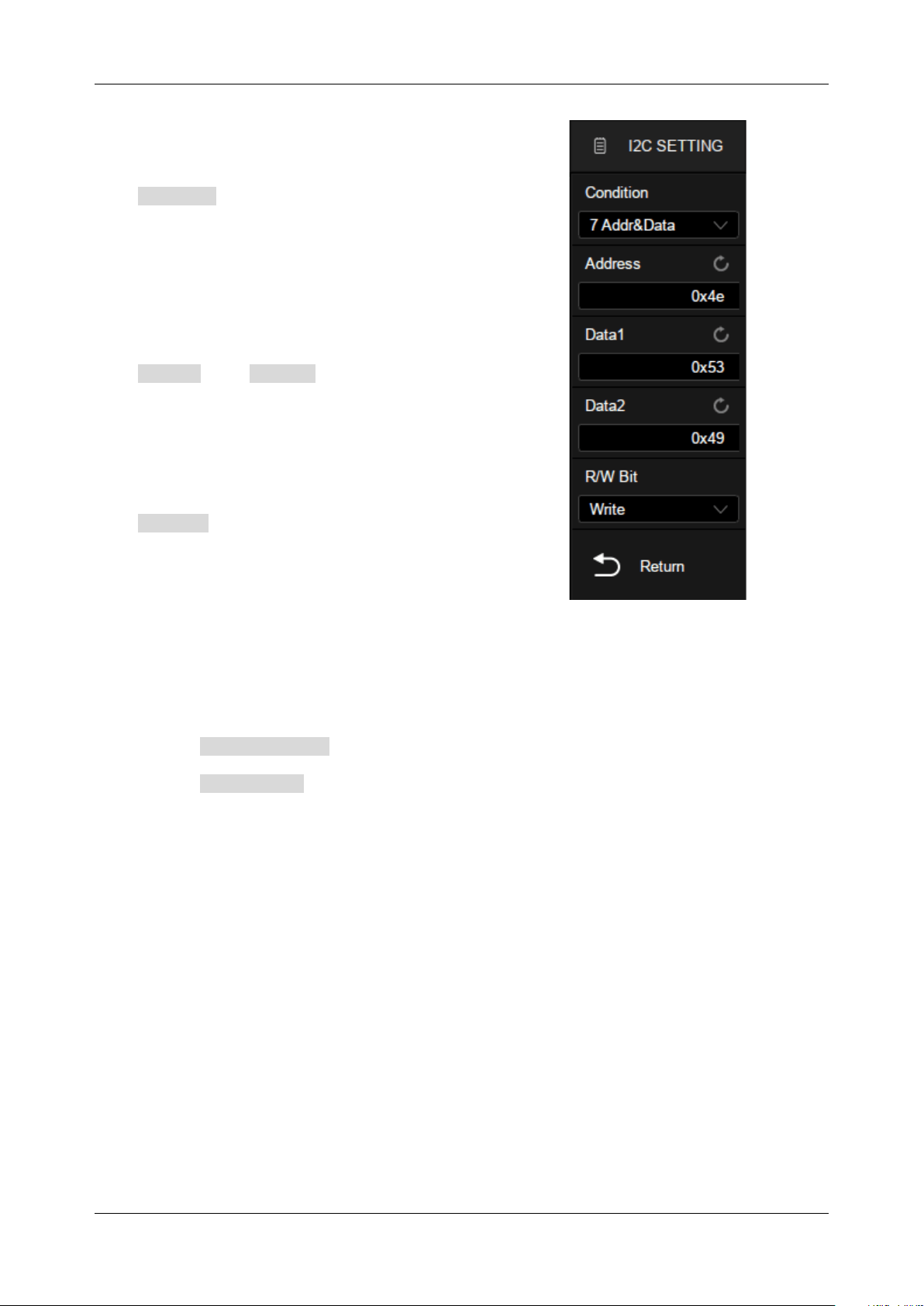
SDS6000L User Manual
int. s i g l e n t . c o m 1 2 1
If you set the trigger condition to 7 address & data or 10
address & data:
Address can be selected in the hexadecimal
range of 0x00 to 0x7F (7-bit) or 0x3FF (10-bit). If the
address is selected as "0xXX (7-bit address)" or
"0xXXX (10-bit address)", the address is ignored. It
will always trigger on the Ack bit followed by the
address.
Data1 and Data2 can be selected in the
hexadecimal range of 0x00 to 0xFF. If the data is
selected as "0xXX", the data is ignored. It will
always trigger on the Ack bit followed by the
address.
R/W Bit can be specified as Write, Read, or Don't
Care.
Data Length
-- The data length range is 1 to 12 bytes. When the SDA data length is equal to the value
of Data Length and address length is the same as the set value, the oscilloscope will be triggered.
Click the Address Length to select "7-bits" or "10-bits" to match the address of the input signal.
Click the Data Length and roll the mouse wheel or use the virtual keypad to set the data length
to match the data length of the input signal.
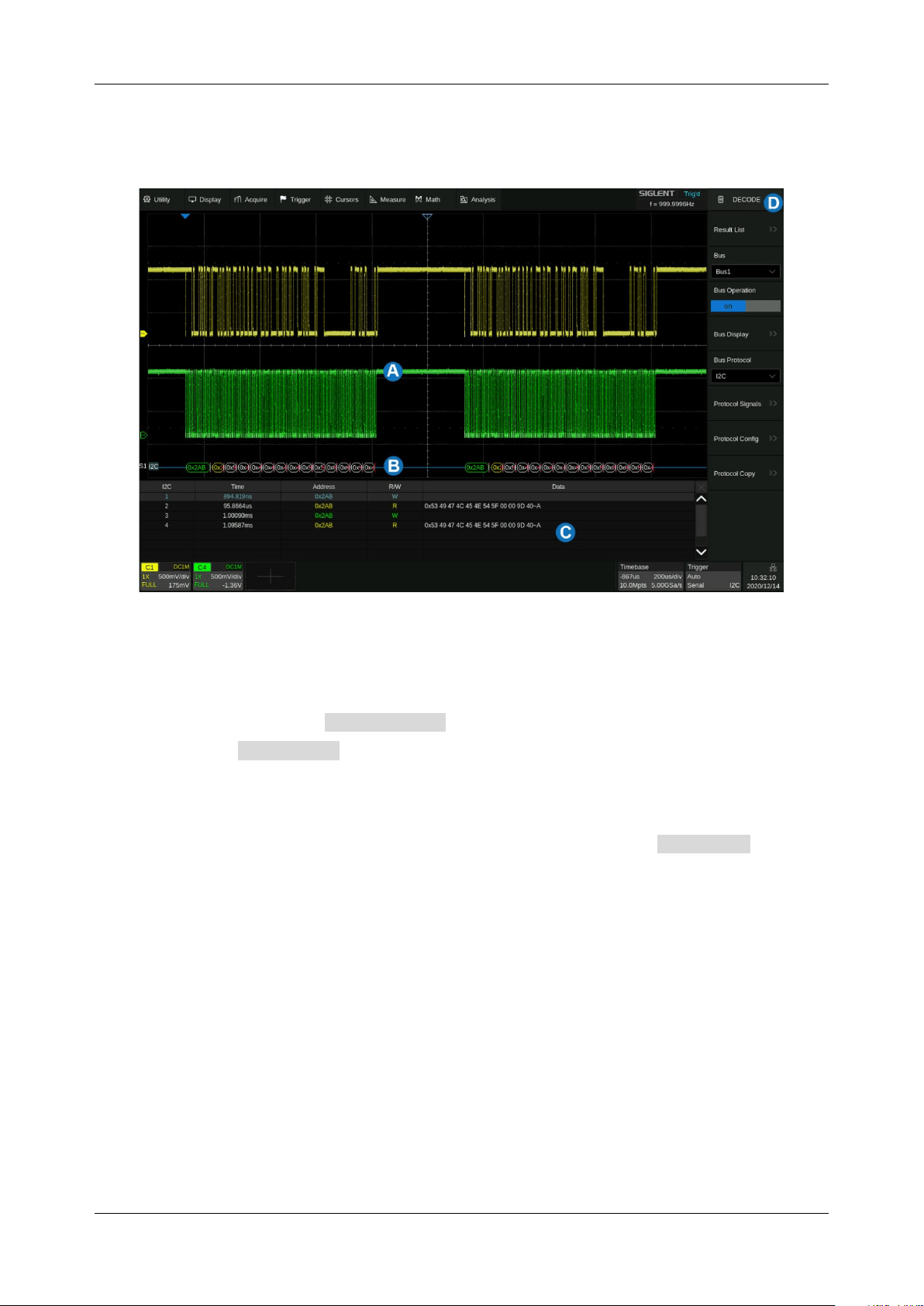
SDS6000L User Manual
1 2 2 i n t . s i g l e n t . c o m
14.2.3 I2C Serial Decode
The layout of the display when I2C decode is enabled is as follows:
A. The waveform display area shows the original waveforms of the bus signals
B. The bus display shows the decoding result of the bus. At most two buses can be decoded at
the same time. Click Bus Operation in the dialog box to turn on or off the selected bus,
and click Bus Display to select the display type of decode result (Binary, Decimal, Hex, or
ASCII).
C. List display area. The decode result of multiple frames can be displayed in the list, in which
each row shows the time label and decode result of a frame. Click Result List to set the
parameters of the list.
D. Decode dialog box
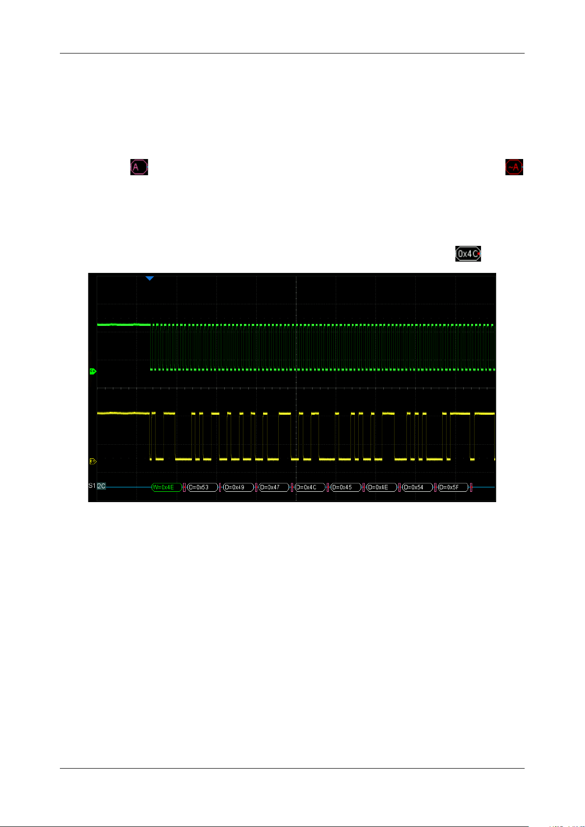
SDS6000L User Manual
int. s i g l e n t . c o m 1 2 3
Bus
The address value is displayed at the beginning of a frame. The write address is displayed
in green and the read address is in yellow.
W/R bit is represented by (W) and (R), followed by the address value.
The after a data or address byte represents ACK (acknowledgment), and
indicates no acknowledgment.
The data value is displayed in white.
A red point at the end of a segment indicates there is not enough space on the display to
show the complete content of a frame, and some content is hidden, such as .
The position of the bus in the vertical direction can be adjusted by dragging with the mouse.
List
TIME -- The horizontal offset of the current data frame head relative to the trigger position.
Address -- Address value. For example, "0x2AB" means that address = 2AB with
acknowledgement.
R/W -- Read or write address.
DATA -- Data bytes.

SDS6000L User Manual
1 2 4 i n t . s i g l e n t . c o m
Configuration
There is only one item Include R/W Bit in the configuration of the I2C decode. When it is disabled,
the address is represented separately from the R/W bit, and when it is enabled, the R/W bit is
represented together with the address.
For example, the address 0x4E: Write: Ack, is displayed as "0x4E (W)" when the R/W bit is not included
and is displayed as "0x9C" when the R/W bit is included.
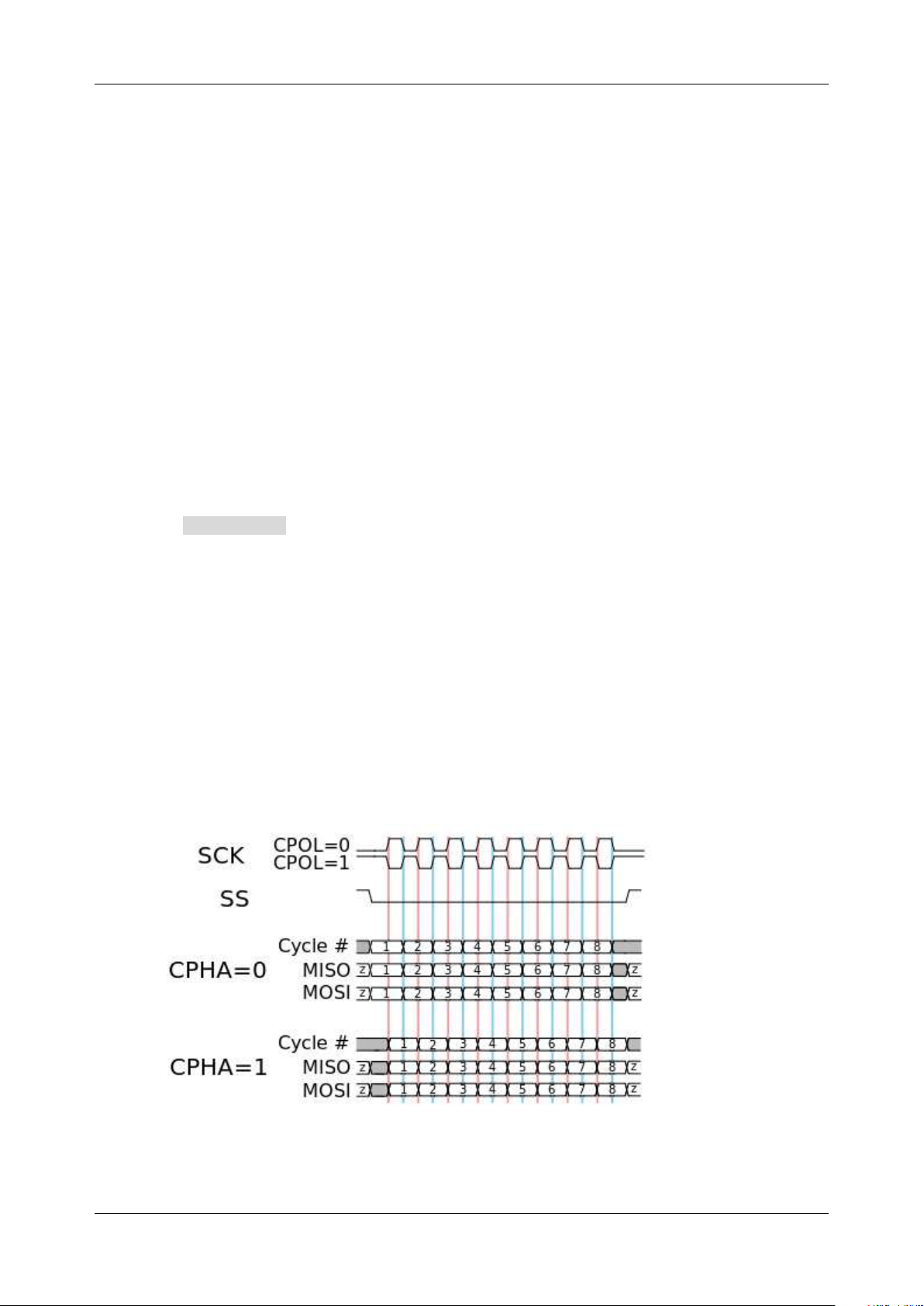
SDS6000L User Manual
int. s i g l e n t . c o m 1 2 5
14.3 SPI Trigger and Serial Decode
This section covers triggering and decoding SPI signals. Please read the following for more details:
"SPI Signal Settings", "SPI Trigger" and "SPI Serial Decode".
14.3.1 SPI Signal Settings
Connect the CLK, MOSI, MISO, and CS signals to the oscilloscope and set the mapping relation
between channels and signals. Then set the threshold level of each signal. The process of specifying
the source and threshold is similar to "I2C Signal Settings".
CLK
In addition to specifying the source and the threshold level, for the CLK signal, it is also necessary to
specify the Edge Select .
Rising–Data latched on the rising edge of the clock.
Falling–Data latched on the falling edge of the clock.
The user can select the edge according to the actual phase relationship between the clock and the
data of the SPI bus. Referring to the following figure, when the falling edge of the clock is aligned with
the data, the rising edge is selected to latch the data. When the rising edge of the clock is aligned with
the data, the falling edge is selected to latch the data.
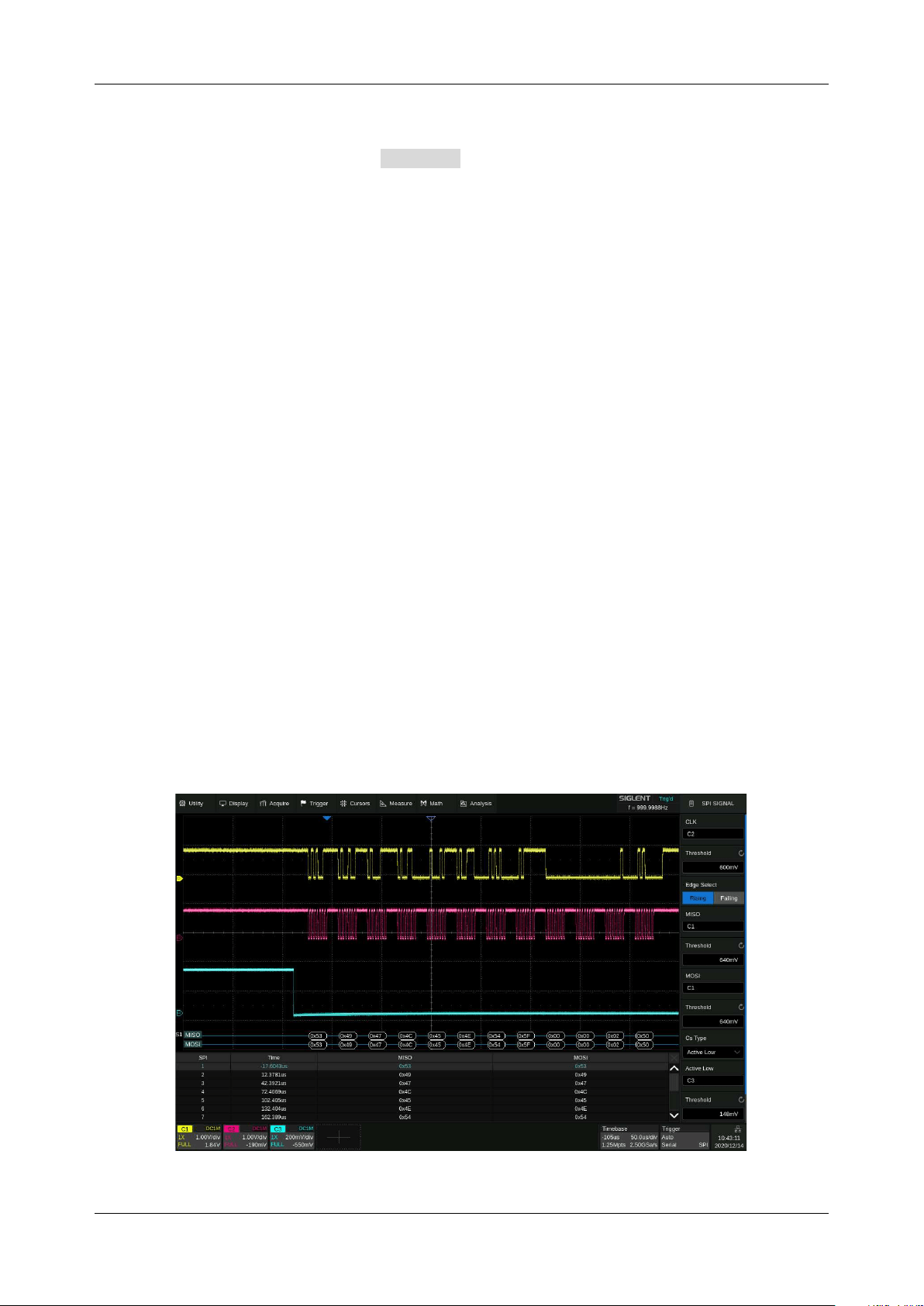
SDS6000L User Manual
1 2 6 i n t . s i g l e n t . c o m
CS
The CS signal should be set to correct CS Type , including CS, ~CS, and Clock Timeout.
CS – Active high. The CS signal needs a complete rising edge in the screen to be regarded as
active.
~CS – Active low. The ~CS signal needs a complete falling edge in the screen to be regarded as
active.
Clock Timeout – It is not necessary to specify the source and the threshold level for the CS signal.
The only parameter for the CS signal is the timeout Limit, which is the minimum time that the clock
signal must be held idle before the oscilloscope acquires valid data. This setting is suitable for the
case where the CS signal is not connected, or the number of oscilloscope channels is insufficient
(such as two-channel oscilloscopes).
The method of copying settings is the same as I2C signal settings. See "I2C Signal Settings" for details.
Example:
Connect the data, CLK, and ~CS signals of an SPI bus respectively to C1, C2, and C3. Data width =
8-bit, Bit order = MSB, CS polarity = active low, and 12 data bytes are transmitted in one frame.
In the SPI trigger signal menu, set the source and threshold of CLK, MISO, and CS signals, then copy
the trigger settings to decoding. Adjust the timebase, so that there is a falling edge on the CS signal
shown on the screen:

SDS6000L User Manual
int. s i g l e n t . c o m 1 2 7
When the CS type is set to Clock Timeout, turn on Cursor, measure the clock idle time between frames
as 150 us, and measure the interval between clock pulses as 1.28 us, then set the timeout to a value
between 1.28 us and 150 us. In this example it is set to 5 us:
If the data width is set to be greater than 8 bits (such as 16 bits), measure the clock idle time between
8-bit data packets as 11.28 us, and then set the timeout time to a value between 11.28 and 150 us. In
this example, it is set to 20 us:
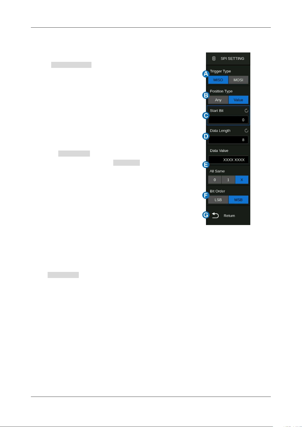
SDS6000L User Manual
1 2 8 i n t . s i g l e n t . c o m
14.3.2 SPI Trigger
The trigger condition for the SPI trigger is mainly about data.
Click Trigger Setting in the dialog box to set data:
A. Trigger Type: MISO or MOSI
B. Set the trigger position type. When set to Any, it will
trigger on the specified data. When set to Value, it
will trigger on the data from the Start Bit
C. Set the start bit of the data value
D. Data Length: 4 ~ 96 bits when the start bit is 0
E. Set to trigger on the specified data value. Click
Data Value twice, and enter the value by the
virtual keypad, or click All Same to set all bits to
0, 1, or ignored ("X")
F. Set the bit order to MSB or LSB
G. Return to the previous menu
14.3.3 SPI Serial Decode
The configuration of SPI decoding is similar to I2C.
In the Bus Config menu, Data Length (4-32 bit) and Bit Order (LSB or MSB) are configurable.
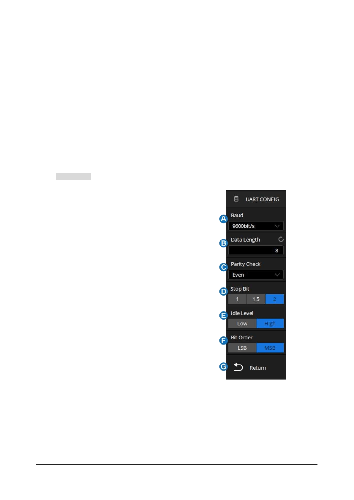
SDS6000L User Manual
int. s i g l e n t . c o m 1 2 9
14.4 UART Trigger and Serial Decode
This section covers triggering and decoding UART signals. Please read the following for more details:
"UART Signal Settings", "UART Trigger" and "UART Serial Decode".
14.4.1 UART Signal Settings
Connect the RX and TX signals to the oscilloscope, set the mapping relation between channels and
signals, and then set the threshold level of each signal. The process of specifying the source and
threshold is similar to "I2C Signal Settings".
In the BusConfig menu of trigger or decode, the following parameters are available:
A. Click to select the baud rate: 600,1200, 2400,
4800, 9600, 19200, 38400, 57600, 115200 b/s
or Custom
B. Data Length: 5~8 bit
C. Parity Check: None, Odd, Even, Mark, or
Space. If the data is 9 bits, the 9
th
bit is treated
as Mark parity or Space parity
D. Select the number of stop bits
E. Set the idle level
F. Set the bit order
G. Return to the previous menu
The method of copying settings is the same as I2C signal settings. See "I2C Signal Settings" for details.
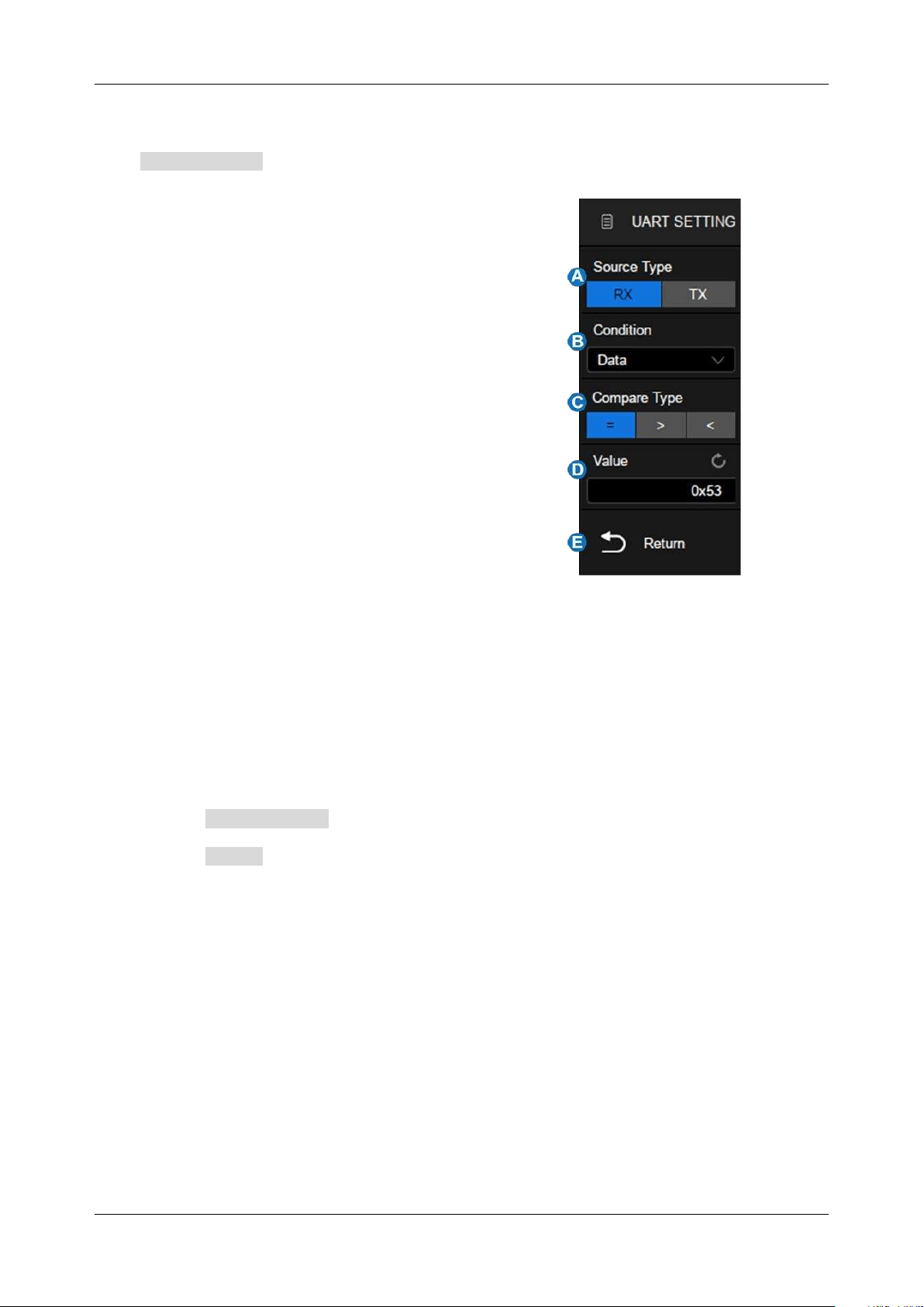
SDS6000L User Manual
1 3 0 i n t . s i g l e n t . c o m
14.4.2 UART Trigger
Click Trigger Setting in the dialog box to set the trigger condition:
A. Source Type: RX or TX
B. Trigger Condition: Start, Stop, Data or Error
C. When the "trigger condition" is Data, set the
compare type to =, >, <
D. When the "trigger condition" is Data, set the
data value
E. Return to the previous menu
Trigger Condition
Start
-- The oscilloscope triggers when the start bit appears on the RX/TX.
Stop
-- The oscilloscope triggers when the stop bits appear on the RX/TX. It always triggers on
the first stop bit.
Data
-- Trigger on data
✓ Click Compare Type to select "=", ">" or "<".
✓ Click Value to set the data value by the mouse wheel or virtual keypad. The range of data
values is 0x00 to 0xff.
Error
-- The oscilloscope performs a parity check on the data according to the parity type set by
the user, and triggers if the check value is incorrect.
14.4.3 UART Serial Decode
The configuration of UART decoding is similar to that of I2C decoding.
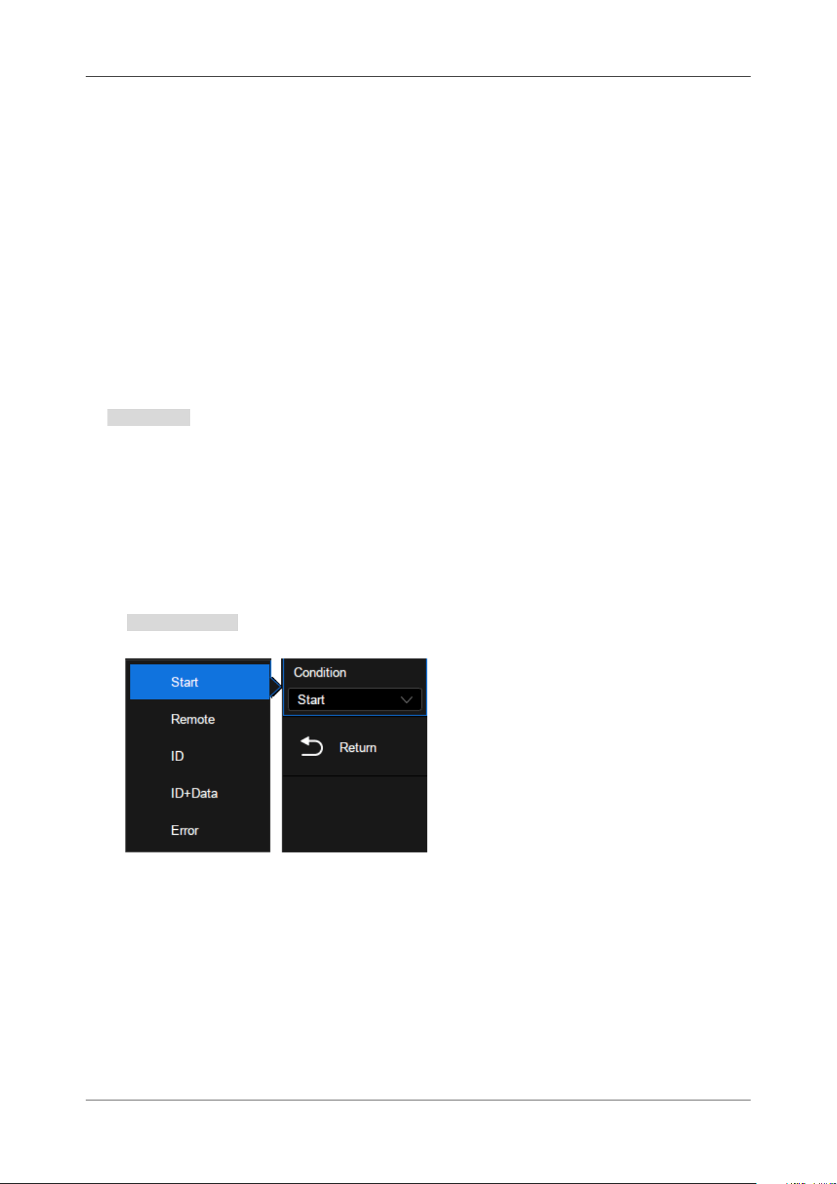
SDS6000L User Manual
int. s i g l e n t . c o m 1 3 1
14.5 CAN Trigger and Serial Decode
This section covers triggering and decoding CAN signals. Please read the following for more details:
"CAN Signal Settings", "CAN Trigger" and "CAN Serial Decode".
14.5.1 CAN Signal Settings
Connect the CAN_H and CAN_L signals to the oscilloscope, set the mapping relation between
channels and signals, and then set the threshold level of each signal. The process of specifying the
source and threshold is similar to "I2C Signal Settings".
In BusConfig menu of trigger and decode, baud rate can be set to: 5 kb/s, 10 kb/s, 20 kb/s, 50 kb/s,
100 kb/s, 125 kb/s, 250 kb/s, 500 kb/s, 800 kb/s, 1 Mb/s or Custom.
The method of copying settings is the same as I2C signal settings. See "I2C Signal Settings" for details.
14.5.2 CAN Trigger
Click Trigger Setting in the CAN trigger dialog box to set the trigger condition:
Start
-- The oscilloscope triggers at the beginning of the frame.
Remote
-- The oscilloscope triggers on a remote frame with a specified ID. ID, ID Bits (11-bit or
29-bit), and Curr ID Byte (1st, 2nd, 3rd, or 4th byte) can be set. Curr ID Byte is used to specify
the byte to be adjusted when using the mouse wheel.
ID
-- The oscilloscope triggers on the data frame that matches the specified ID. ID, ID Bits (11-bit
or 29-bit), and Curr ID Byte (1st, 2nd, 3rd, or 4th byte) can be set.
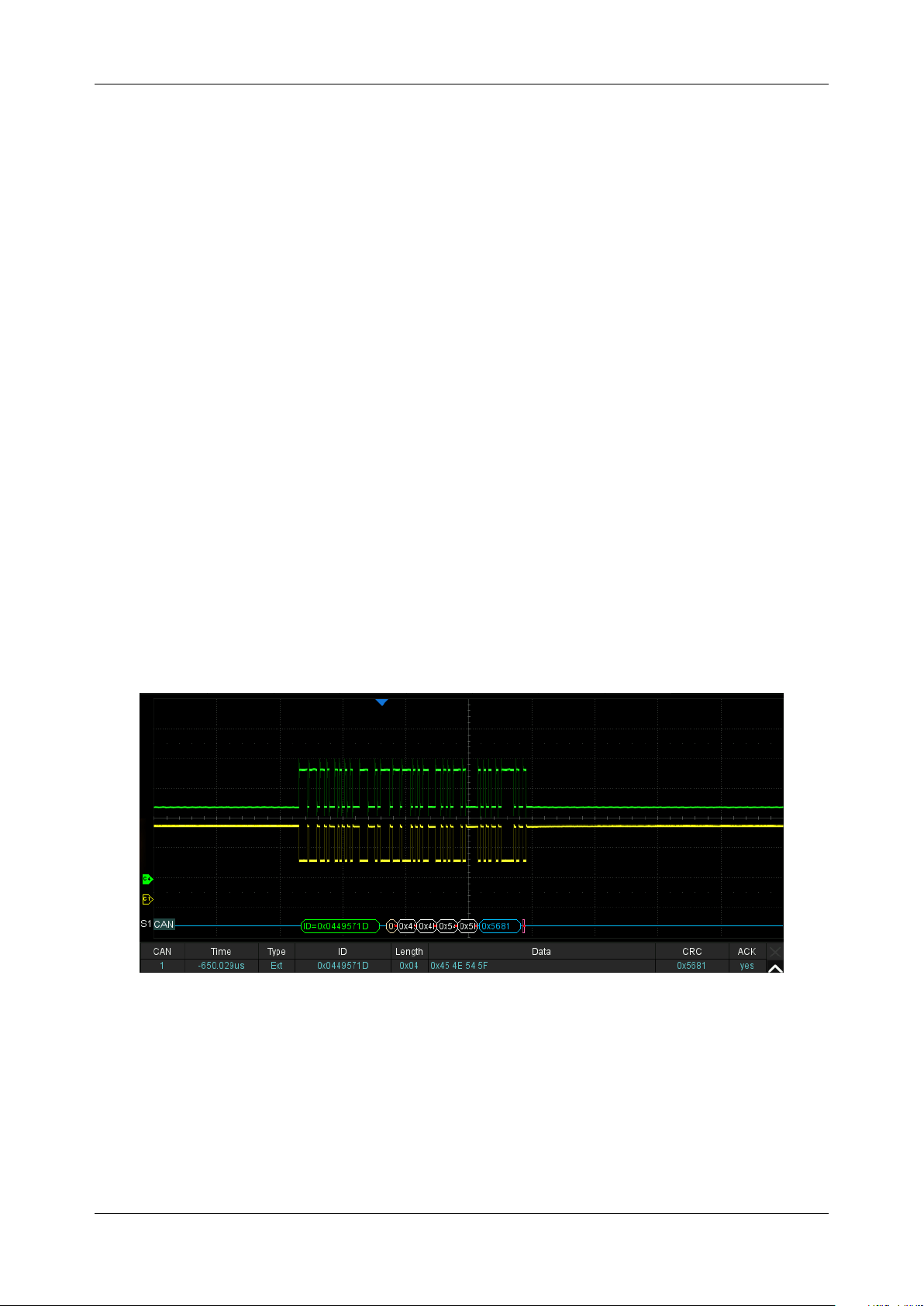
SDS6000L User Manual
1 3 2 i n t . s i g l e n t . c o m
ID + Data
-- The oscilloscope triggers on the data frame that matches the specified ID and
data.ID, ID Bits (11-bit or 29-bit), Curr ID Byte (1st, 2nd, 3rd, or 4th byte), Data1, and Data2 can
be set.
Error
-- The oscilloscope triggers on the error frame.
14.5.3 CAN Serial Decode
The configuration of CAN decoding is similar to that of I2C decoding.
On the bus:
ID is displayed in green.
LEN (data length) is displayed in light yellow.
DATA are displayed in white.
CRC is displayed in blue.
The red point at the end of a segment indicates there is not enough space on the display to
show the complete content of a frame and some content is hidden.
In the list view:
Time -- The horizontal offset of the current data frame head relative to the trigger position.
Type -- Type of the frame. The Data frame is represented by “D” and the remote frame is
represented by “R”.
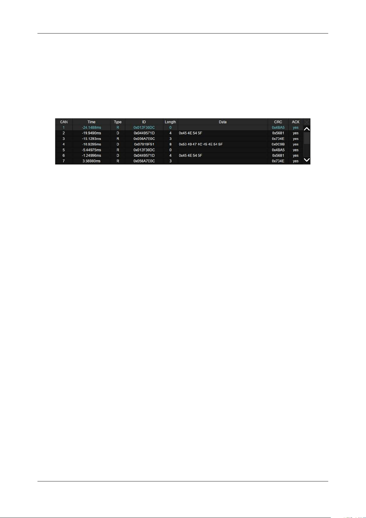
SDS6000L User Manual
int. s i g l e n t . c o m 1 3 3
ID -- ID of the frame, 11-bits or 29-bits ID are automatically detected.
Length -- Data length.
Data -- Data values.
CRC -- Cycle redundancy check.
Ack -- Acknowledge bit.
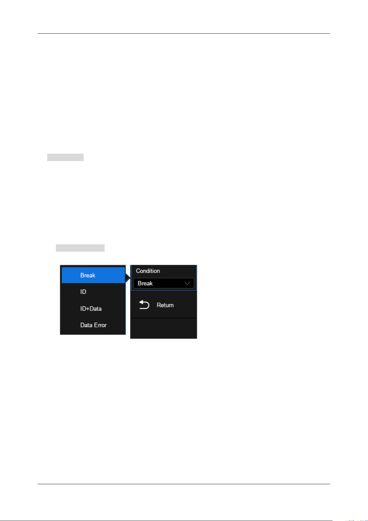
SDS6000L User Manual
1 3 4 i n t . s i g l e n t . c o m
14.6 LIN Trigger and Serial Decode
This section covers triggering and decoding LIN signals. Please read the following for more details:
“LIN Signal Settings”, “LIN Trigger” and “LIN Serial Decode”.
14.6.1 LIN Signal Settings
Connect the LIN signal to the oscilloscope, and then set the threshold level of the signal. The process
of specifying the source and threshold is similar to “I2C Signal Settings”.
In BusConfig menu of trigger and decode, baud rate can be set to: 600 b/s,1200 b/s, 2400 b/s, 4800
b/s, 9600 b/s, 19200 b/s or Custom.
The method of copying settings is the same as I2C signal settings. See “I2C Signal Settings” for details.
14.6.2 LIN Trigger
Click Trigger Setting in the LIN trigger dialog box to set the trigger conditions:
Break
-- The oscilloscope triggers at the beginning of the frame.
ID
-- The oscilloscope triggers on the frame that matches the specified ID, which ranges from 0x00
to 0x3f.
ID & Data
-- The oscilloscope triggers on the frame that matches the specified ID and data.ID,
Data1, and Data2 can be set.
Data Error
-- The oscilloscope will trigger when a data error happens.
SDS6000L User Manual
int. s i g l e n t . c o m 1 3 5
14.6.3 LIN Serial Decode
The configuration of LIN decoding is similar to that of I2C decoding.
On the bus:
ID is displayed in green
LEN (data length) and CHK are displayed in blue
DATA are displayed in white.
In the list view:
Time -- The horizontal offset of the current data frame head relative to the trigger position.
ID -- ID of the frame.
Data length -- Data length.
ID Parity -- ID parity check.
Data -- Data values.
Checksum -- Data checksum.
SDS6000L User Manual
1 3 6 i n t . s i g l e n t . c o m
14.7 FlexRay Trigger and Serial Decode
This section covers triggering and decoding FlexRay signals. Please read the following for more details:
"FlexRay Signal Settings", "FlexRay Trigger" and "FlexRay Serial Decode".
14.7.1 FlexRay Signal Settings
Connect the FlexRay signal to the oscilloscope, and then set the threshold level of the signal. The
process of specifying the source and threshold is similar to "I2C Signal Settings".
In the BusConfig menu of the trigger and decode, the baud rate can be set to: 2.5 Mb/s, 5.0 Mb/s,
10.0 Mb/s, or Custom.
The method of copying settings is the same as I2C signal settings. See "I2C Signal Settings" for details.
14.7.2 FlexRay Trigger
Click Trigger Setting in the FlexRay trigger dialog box to set the trigger conditions:
TSS
-- The oscilloscope triggers on the transmission start sequence.
Frame
-- The oscilloscope triggers on the frame.
✓ Set Frame header indicators: Payload preamble indicator, null frame indicator, sync frame
indicator, startup frame indicator.
✓ Click ID to set the frame ID by the mouse wheel or virtual keypad. The range of ID is 0x000
to 0x7ff.
✓ Click Compare Type to select "=", ">" or "<". When setting the Compare Type as "=",
SDS6000L User Manual
int. s i g l e n t . c o m 1 3 7
the repetition factor is also required.
✓ Click Cycle to set the cycle count by the mouse wheel or virtual keypad. The range of data
values is 0 to 63.
Symbol
-- The oscilloscope triggers on CAS/MTS (Conflict Avoidance Symbol/ Media access Test
Symbol) or WUS (Wake-up Symbol)
Errors
-- The oscilloscope will trigger when a data error happens, including errors on FSS, BSS,
FES, Header CRC, and Frame CRC.
14.7.3 FlexRay Serial Decode
The configuration of FlexRay decoding is similar to that of I2C decoding.
On the bus:
The signatures (CAS/MTS, WUP) are displayed in yellow-green.
TSS transmission start sequence, displayed in yellow-green. The null frame indicator, the
Sync frame indicator, and the Startup frame indicator are displayed in the frame and
displayed in pink.
The ID is displayed in the frame and is displayed in green.
PL (Valid Data Length) is displayed in frames, in words, and in light yellow.
HCRC (Head Check Code) is displayed in the frame and displayed in blue.
CYC (cycle) is displayed in the frame and displayed in light yellow.
D (data) is displayed in the frame and displayed in white.
FCRC (Data Check Code) is displayed in the frame and displayed in blue.
SDS6000L User Manual
1 3 8 i n t . s i g l e n t . c o m
In the list view:
Time -- The horizontal offset of the current data frame head relative to the trigger position.
FID -- Frame ID, the symbol occupies a single line of the list.
PL -- Valid Data Length
HCRC -- Head Check Code
CYC -- Cycle count
Data -- Data values
FCRC -- Data Check Code
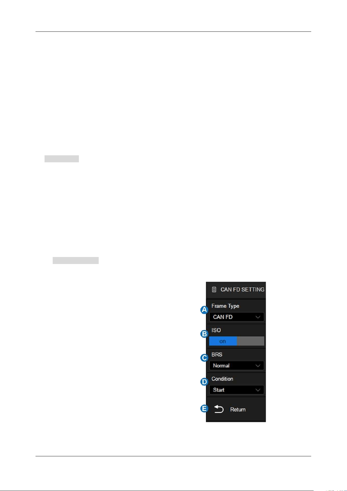
SDS6000L User Manual
int. s i g l e n t . c o m 1 3 9
14.8 CAN FD Trigger and Serial Decode
This section covers triggering and decoding CAN FD signals. Please read the following for more details:
"CAN FD Signal Settings", "CAN FD Trigger" and "CAN FD Serial Decode".
14.8.1 CAN FD Signal Settings
Connect the CAN FD signal to the oscilloscope, and then set the threshold level of the signal. The
process of specifying the source and threshold is similar to "I2C Signal Settings".
In BusConfig menu of trigger and decode, the nominal baud rate can be set to: 10 kb/s, 25 kb/s, 50
kb/s, 100 kb/s, 250 kb/s, 1 Mb/s or Custom. The data baud rate can be set to: 500 kb/s, 1 Mb/s, 2 Mb/s,
5 Mb/s, 8 Mb/s, 10 Mb/s or Custom.
The method of copying settings is the same as I2C signal settings. See "I2C Signal Settings" for details.
14.8.2 CAN FD Trigger
Click Trigger Setting in the CAN FD trigger dialog box to set the trigger conditions:
A. Frame Type: Both, CAN, CAN FD
B. When the "Frame Type" is CAN FD,
turn on or off ISO
C. When the "Frame Type" is CAN FD,
set the BRS (Bit Rate Switch) to Both,
Normal or FD
D. Trigger Condition: Start, Remote, ID,
ID + Data, Error
E. Return to the previous menu

SDS6000L User Manual
1 4 0 i n t . s i g l e n t . c o m
Trigger Condition
Start
-- The oscilloscope triggers at the beginning of the frame.
Remote
-- The oscilloscope triggers on a remote frame with a specified ID. ID, ID Bits (11-bit or
29-bit), and Curr ID Byte (1st, 2nd, 3rd, or 4th byte) can be set. Curr ID Byte is used to specify the
byte to be adjusted when using the mouse wheel.
ID
-- The oscilloscope triggers on the data frame that matches the specified ID. ID, ID Bits (11-bit
or 29-bit), and Curr ID Byte (1st, 2nd, 3rd, or 4th byte) can be set.
ID + Data
-- The oscilloscope triggers on the data frame that matches the specified ID and data.ID,
ID Bits (11-bit or 29-bit), Curr ID Byte (1st, 2nd, 3rd, or 4th byte), Data1, and Data2 can be set.
Error
-- The oscilloscope triggers on the error frame.
✓ Error Frame
✓ Stuff Bit Error
✓ CRC Mismatch Error: The oscilloscope triggers when the calculated CRC does not match the
transmitted CRC.
✓ Stuff Bit Cnt Err: Effective only when ISO is turned on, the oscilloscope triggers when the stuff
bit count is incorrect.
✓ Stuff Bit Cnt Par. Err: Effective only when ISO is turned on, the oscilloscope triggers when the
polarity of the stuff bit count is incorrect.
14.8.3 CAN FD Serial Decode
The configuration of CAN FD decoding is similar to that of I2C decoding.
On the bus:
ID is displayed in green.
BRS (Bit Rate Switch) is displayed in light yellow.
ESI (Error State Indicator) is displayed in blue.
L (Data Length) is displayed in light yellow.
D (Data) is displayed in white.
CRC is displayed in blue.
Ack is displayed in pink.
The red point at the end of a segment indicates there is not enough space on the display to
show the complete content of a frame and some content is hidden.
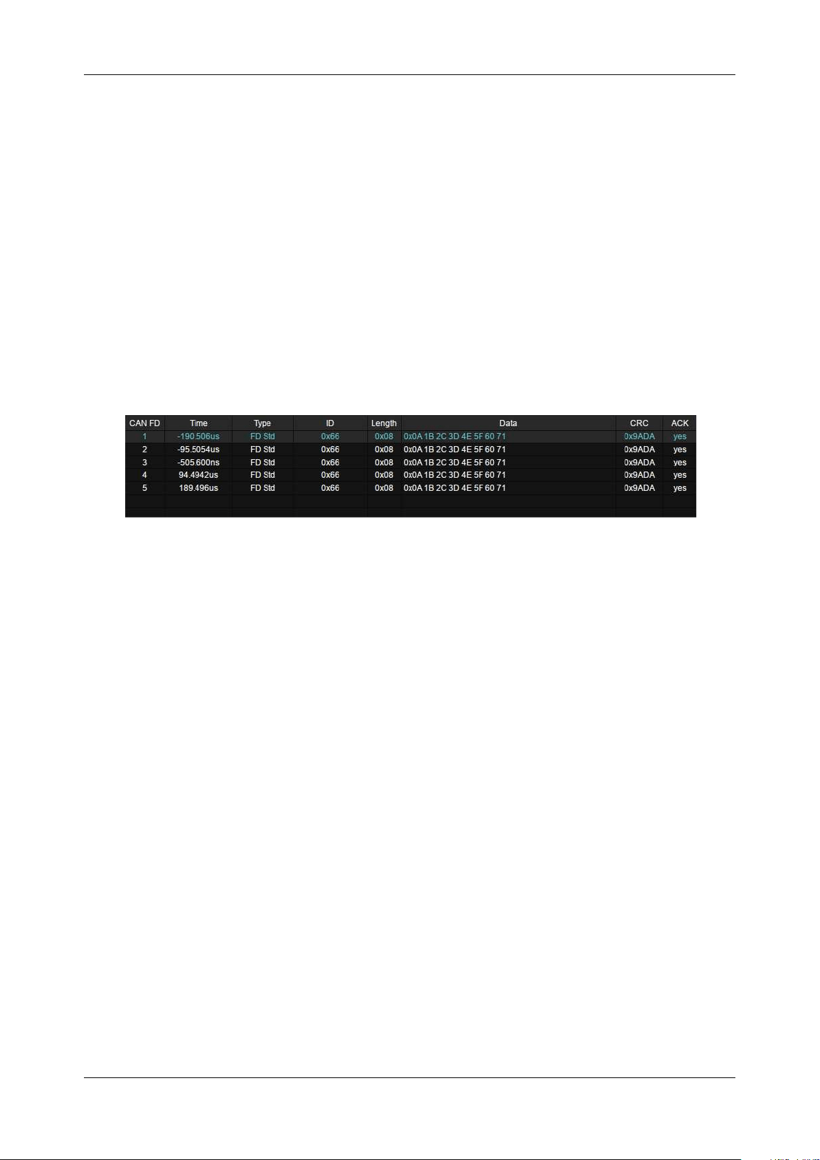
SDS6000L User Manual
int. s i g l e n t . c o m 1 4 1
In the list view:
Time -- The horizontal offset of the current data frame head relative to the trigger position.
Type -- Type of the frame. The Standard CAN frame is represented by "Std", CAN FD frame
is represented by "FD", the extended frame is represented by "Ext" and the remote frame is
represented by "RTR".
ID -- Frame ID.
Length -- Data length.
Data -- Data bytes.
CRC -- Cycle redundancy check.
Ack -- Acknowledge bit.

SDS6000L User Manual
1 4 2 i n t . s i g l e n t . c o m
14.9 I2S Trigger and Serial Decode
This section covers triggering and decoding I2S signals. Please read the following for more details:
"I2S Signal Settings", "I2S Trigger" and "I2S Serial Decode".
14.9.1 I2S Signal Settings
Connect the WS, BCLK, and Data signals to the oscilloscope, set the mapping relation between
channels and signals, and then set the threshold level of each signal. The process of specifying the
source and threshold is similar to "I2C Signal Settings"
BCLK
In addition to specifying the source and the threshold level, BCLK signals also require the specification
of the Edge Select .
Rising– Data latched on the rising edge of the clock.
Falling– Data latched on the falling edge of the clock.
WS
In addition to specifying the source and the threshold level, WS signals also require the specification
of the Left CH .
Low– Select the left channel when WS is low and the right channel when WS is high.
High– Select the right channel when WS is low and the left channel when WS is high.
The method of copying settings is the same as I2C signal settings. See "I2C Signal Settings" for details.
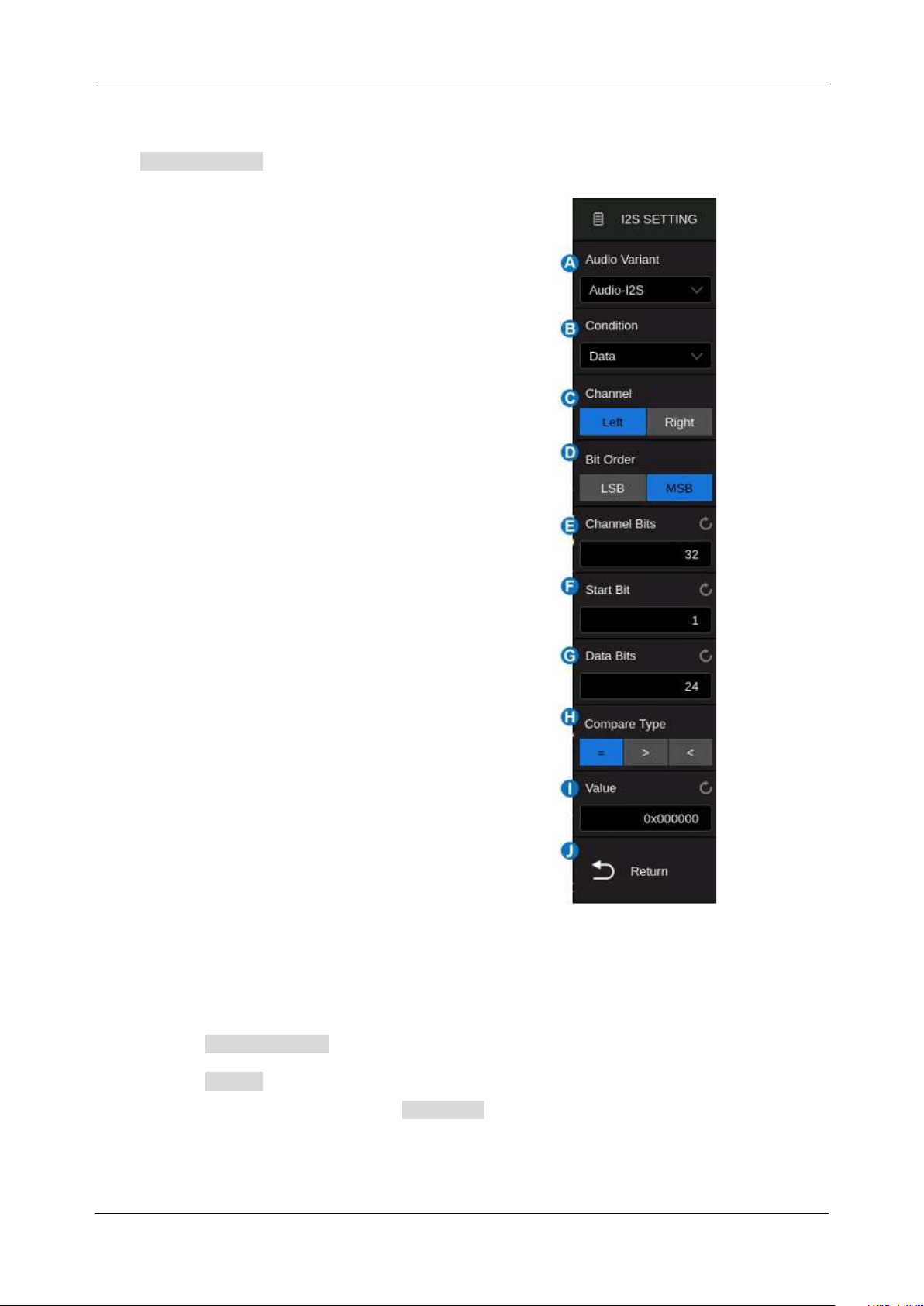
SDS6000L User Manual
int. s i g l e n t . c o m 1 4 3
14.9.2 I2S Trigger
Click Trigger Setting in the I2S trigger dialog box to set the trigger conditions :
A. Audio Variant: Audio-I2S, Audio-LJ,
Audio-RJ
B. Trigger Condition: Data, Mute, Clip,
Glitch, Rising Edge, Falling Edge
C. Channel: Set the channel to trigger, Left
or Right
D. Set the bit order to MSB or LSB
E. Channel Bits: Specify the receiver word
length. The range is from 1 to 32 bits
F. Start Bit: The start bit of data, ranging
from 0 to 31
G. Data Bits: Specify the number of bits per
word. It should be less than the channel
bits
H. When the "Trigger Condition" is Data, set
the compare type to =, >, <
I. When the "Trigger Condition" is Data, set
the data value
J. Return to the previous menu
Trigger Condition
Data
-- Trigger on data.
✓ Click Compare Type to select "=", ">" or "<".
✓ Click Value to set the data value by the mouse wheel or virtual keypad. The range of data
value is related to the number of Data Bits .
Mute
--
Trigger on the mute signal. Mute signal: Volume is less than the set value and duration
reaches the set value.
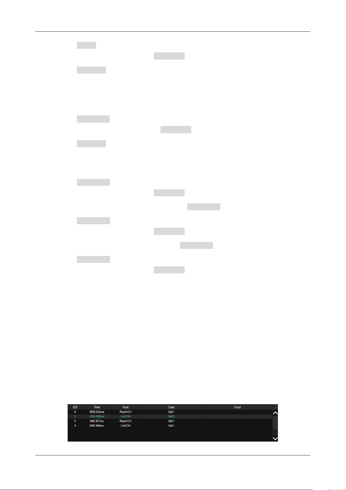
SDS6000L User Manual
1 4 4 i n t . s i g l e n t . c o m
✓ Click MNF to set the mute threshold by the mouse wheel or virtual keypad. The range of
values is related to the number of Data Bits .
✓ Click Duration to set the value by the mouse wheel or virtual keypad. The range is 1-64
frames.
Clip
--
Trigger on the clipped signal. Clip signal: Volume is greater than the set value and duration
reaches the set value.
✓ Click Clip Level to set the clip threshold by the mouse wheel or virtual keypad. The range
of values is related to the number of Data Bits .
✓ Click Duration to set the value by the mouse wheel or virtual keypad. The range is 1-64
frames.
Glitch
--
Trigger on glitches within the audio signal.
✓ Click Threshold to set the threshold by the mouse wheel or virtual keypad. The range of
values is related to the number of Data Bits .
Rising Edge
--
Trigger on signals greater than the Threshold setting value.
✓ Click Threshold to set the threshold by the mouse wheel or virtual keypad. The range of
values is related to the number of Data Bits .
Falling Edge
--
Trigger on signals less than the Threshold setting value.
✓ Click Threshold to set the threshold by the mouse wheel or virtual keypad. The range of
values is related to the number of Data Bits .
14.9.3 I2S Serial Decode
The configuration of I2S decoding is similar to that of I2C decoding.
In the list view:
Time -- The horizontal offset of the current data frame head relative to the trigger position.
Type -- Channel type, the left channel is represented by "Left CH" and the right channel is
represented by "Right CH".
Data -- Data bytes
Error -- Error
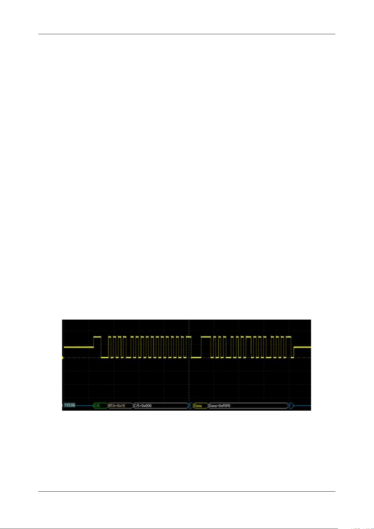
SDS6000L User Manual
int. s i g l e n t . c o m 1 4 5
14.10 MIL-STD-1553B Trigger and Serial Decode
This section covers triggering and decoding MIL-Standard 1553B signals. Please read the following
for more details: "MIL-STD-1553B Signal Settings" and "MIL-STD-1553B Serial Decode".
14.10.1 MIL-STD-1553B Signal Settings
Connect the MIL-STD-1553B signal to the oscilloscope, set the mapping relation between channels
and signals, and then set the threshold level of each signal. The process of specifying the source and
threshold is similar to "I2C Signal Settings"
14.10.2 MIL-STD-1553B Serial Decode
The configuration of MIL-STD-1553B decoding is similar to that of I2C decoding.
On the bus:
C/S the Command/Status word is displayed in green.
RTA the RT address is displayed in the frame and displayed in light yellow.
C/S Data is displayed in the frame and is displayed in white.
The data word is displayed in yellow and the data is displayed in the frame and displayed in
white.
The Check Code is displayed in the frame and displayed in blue.
In the decoding list view:
Time— The horizontal offset of the current data frame head relative to the trigger position.
RTA— The RT address
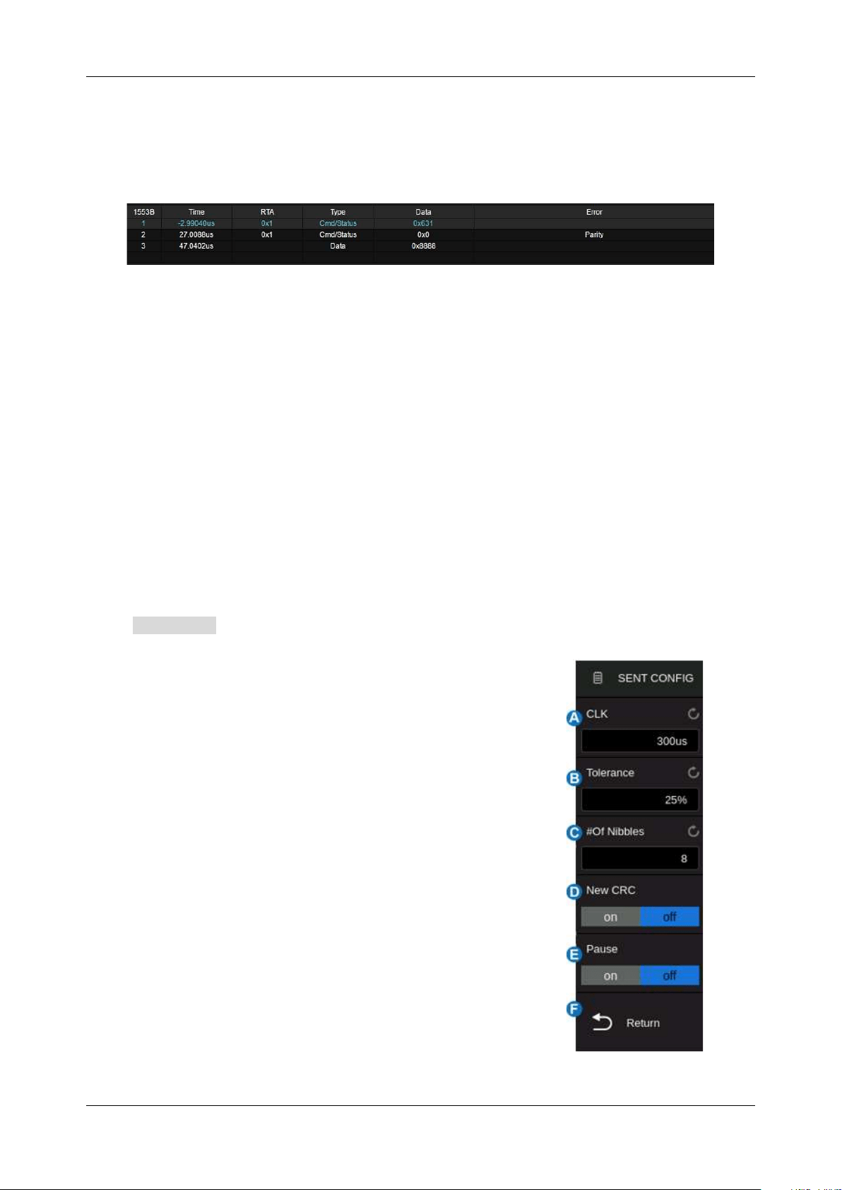
SDS6000L User Manual
1 4 6 i n t . s i g l e n t . c o m
Type— Type of the word
Data— Data values
Error— Error type
14.11 SENT Trigger and Serial Decode
This section covers triggering and decoding SENT signals. Please read the following for more details:
"SENT Signal Settings", "SENT Trigger" and "SENT Serial Decode".
14.11.1 SENT Signal Settings
Connect the SENT signal to the oscilloscope, set the mapping relation between channels and signals,
and then set the threshold level of each signal. The process of specifying the source and threshold is
similar to "I2C Signal Settings"
In the BusConfig menu of trigger or decode, the following parameters are available:
A. Click to specify the nominal clock period (tick) time
B. Set the percent tolerance to determine whether the sync
pulse is valid for decoding the data
C. Set the number of nibbles in a Fast Channel Message
D. Set the CRC format that will be used in calculating the
correctness of the CRCs. The New CRC selection uses the
2010 CRC format. If “NEW” is not selected, the CRC will
use the 2008 format. Enhanced Serial Message CRCs are
always calculated using the 2010 format, but for the Fast
Channel Messages, and Short Serial Message CRCs, the
chosen setting is used
E. Specify whether there is a pause pulse between Fast
Channel Messages
F. Return to the previous menu
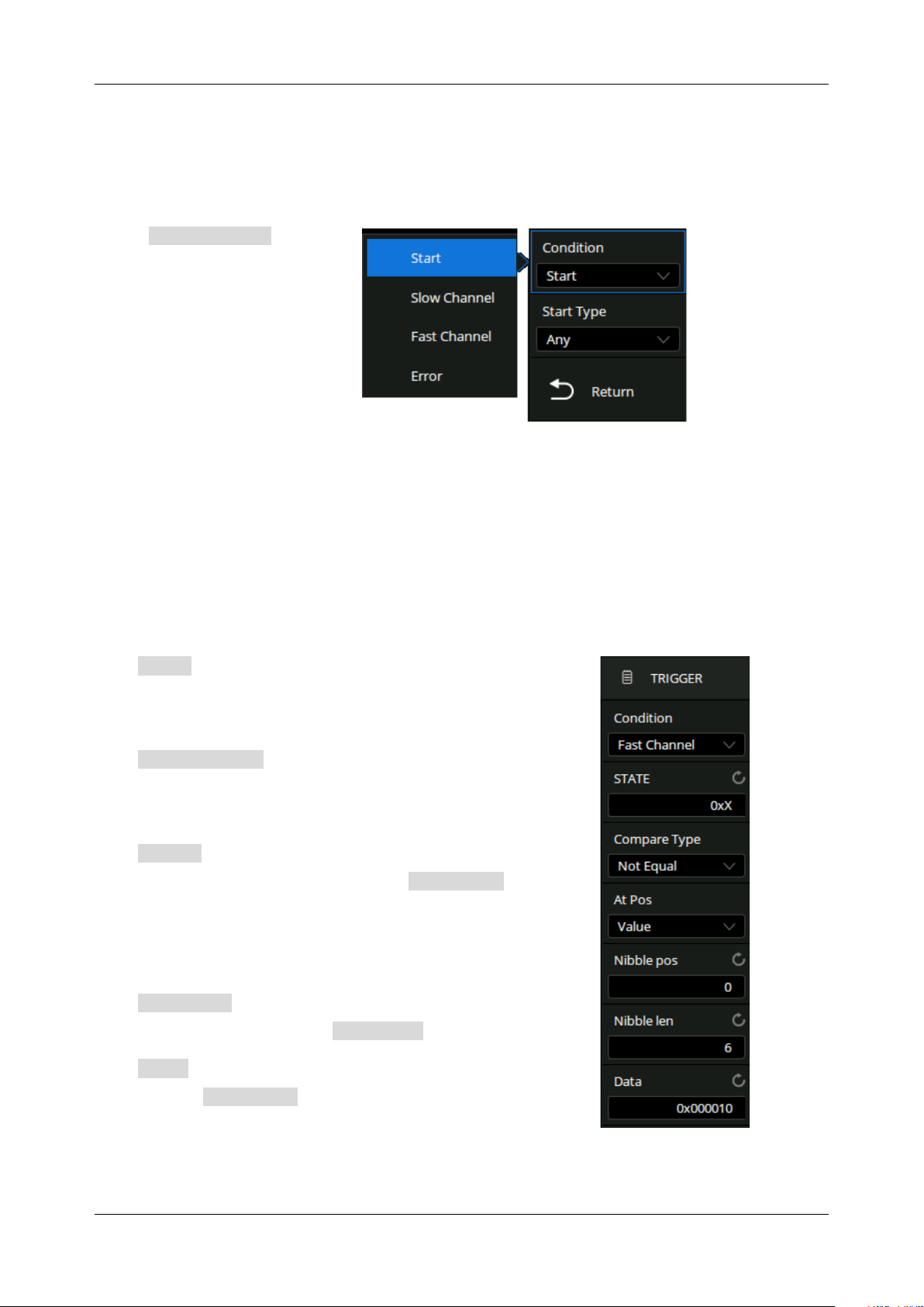
SDS6000L User Manual
int. s i g l e n t . c o m 1 4 7
14.11.2 SENT Trigger
When the protocol is set to SENT, the following trigger conditions can be set: Start, Slow Channel, Fast
Channel, and Error.
Click Trigger Setting in the
SENT trigger dialog box to
select the trigger condition:
Start
-- The oscilloscope will be triggered at the start of the message (after 56 synchronization ticks).
You can select the type of message: Fast Channel Message, Slow Channel Message, or any.
Fast Channel
-- The oscilloscope will be triggered on a Fast Channel Message when the Status &
Communication nibble and the data nibbles match the specified values.
State can be selected in the hexadecimal range of 0x0
to 0xF. If the value is selected as "0xX", the state is
ignored.
Compare Type can be specified as Equal, Not Equal,
Less than, Less or Equal, Greater than, Greater or Equal,
in Range of, or out of Range.
At Pos determines the start position of the trigger data.
If selected as Value, you need to set Nibble Pos in the
decimal range of 0 to 5. If selected as Don’t care, the
oscilloscope will be triggered at the first data which
matches the specified condition.
Nibble Len can be selected in the decimal range of 1 to
6. It is associated with the Nibble Pos .
Data can be selected in hex. The range is associated
with the Nibble Pos . If the data is selected as "0xXX",
the data is ignored.
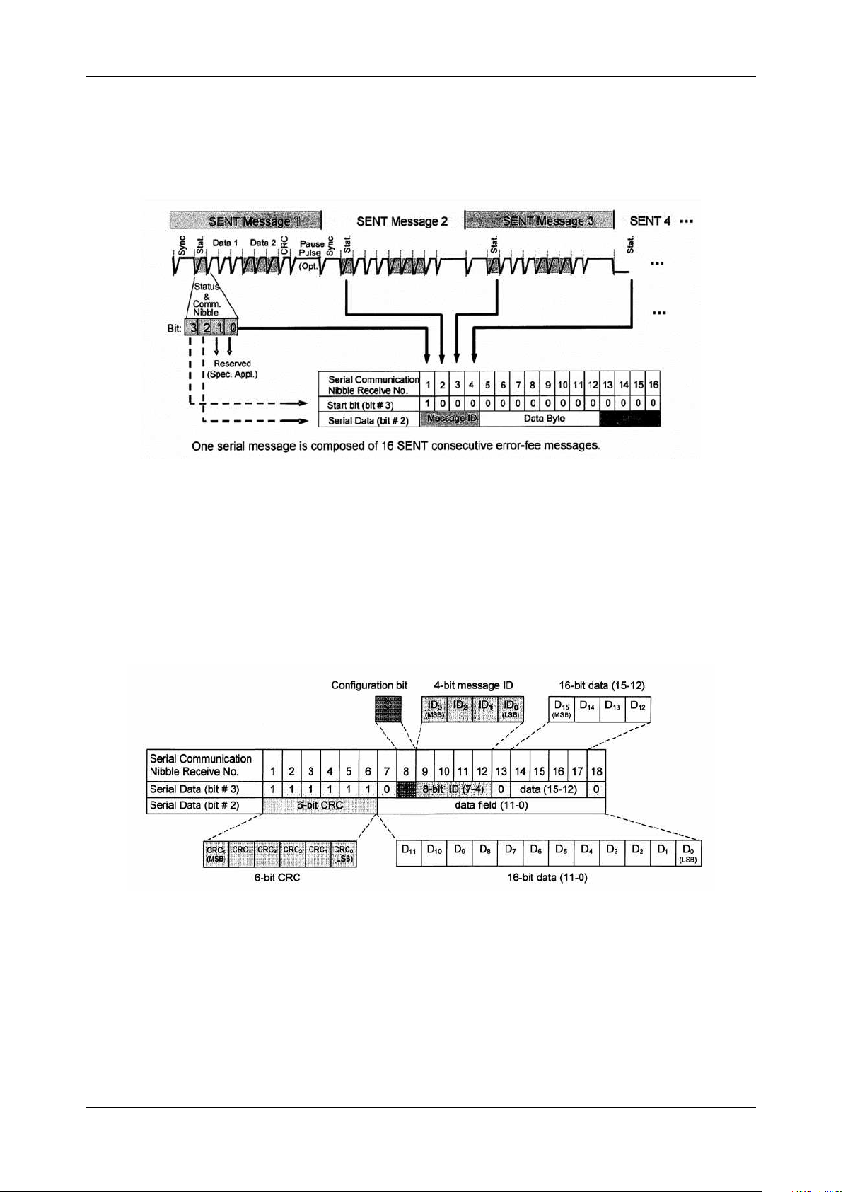
SDS6000L User Manual
1 4 8 i n t . s i g l e n t . c o m
Slow Channel
-- the oscilloscope will be triggered on a Slow Channel Message.
Frame (short serial message) -- The 16-bit message consists of a 4-bit Message ID nibble, 2 nibbles
(1 byte) of data, and a CRC checksum nibble. If ID and data match, then trigger on the end of CRC bit.
The serial message frame contains 21 bits of payload data. Two different configurations can be chosen
and determined by the configuration bit (serial data bit #3, serial communication nibble No. 8):
Frame (enhanced serial message with 4bits ID) --16-bit data and 4-bit message ID, the configuration
bit is 1.
Frame (enhanced serial message with 8bits ID) —12-bit data and 8-bit message ID, the configuration
bit is 0.
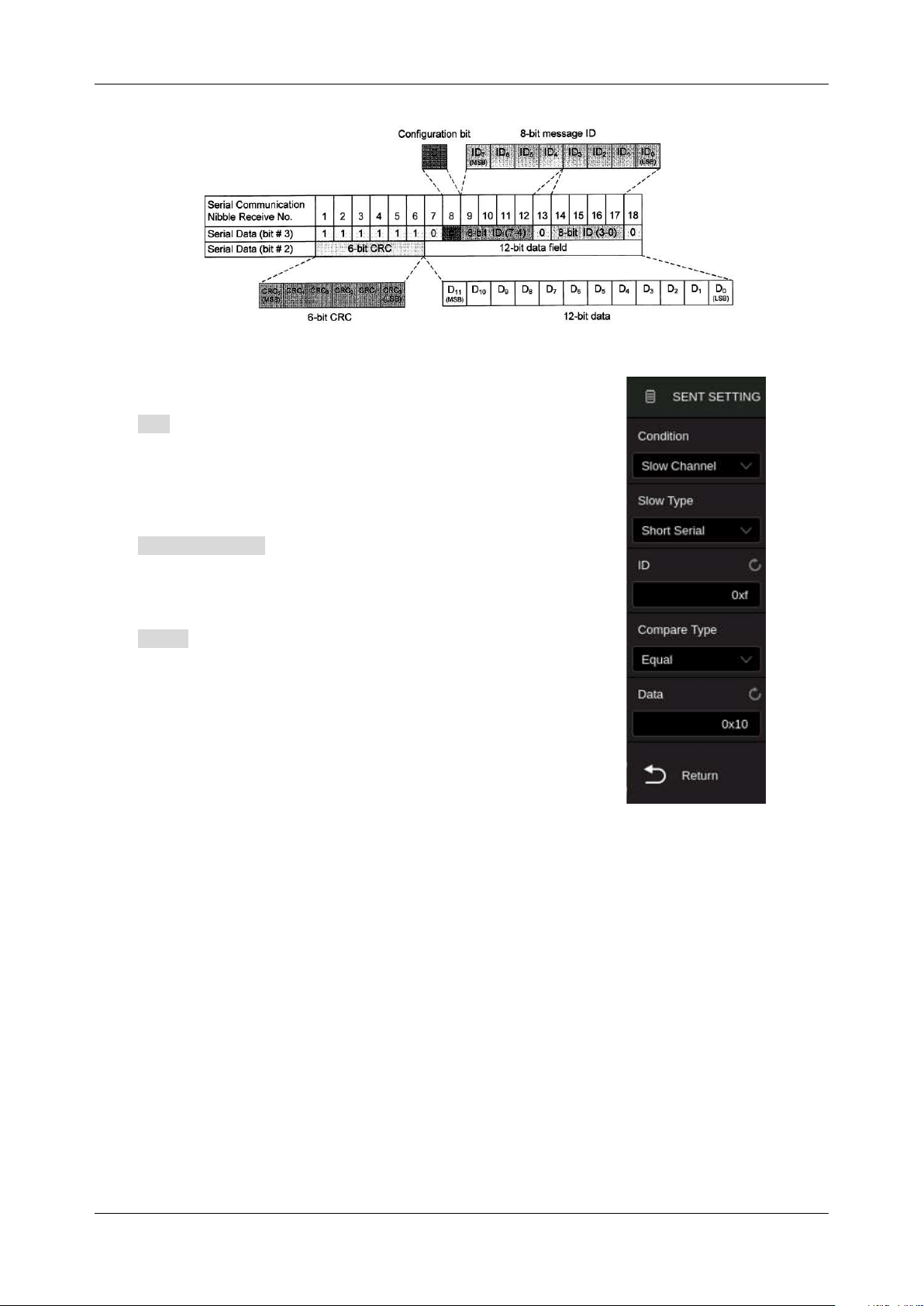
SDS6000L User Manual
int. s i g l e n t . c o m 1 4 9
If you set the trigger condition to Slow Channel:
ID can be selected in the hexadecimal range of 0x0 to
0xF (short serial / enhanced serial with 4 bits ID) or 0x00 to
0xFF (enhanced serial with 8 bits ID). If it is selected as
"0xXX", the ID is ignored.
Compare Type can be specified as Equal, Not Equal,
Less than, Less or Equal, Greater than, Greater or Equal,
in Range of, or out of Range.
Data can be selected in the hexadecimal range of 0x00
to 0xFF (short serial) or 0x0000 to 0xFFFF (enhanced serial
with 4 bits ID) or 0x000 to 0Xfff (enhanced serial with 8 bits
ID). If it is selected as "0xXX", the data is ignored.
Error
-- The oscilloscope triggers on the error frame. Errors include Successive Sync Pulses Error,
Pulse Period Error, Fast Channel CRC Error, Slow Channel CRC Error, All CRC Errors.
Successive Sync Pulses Error: Triggers on a sync pulse whose width varies from the previous
sync pulse's width by greater than 1/64 (1.5625%, as defined in the SENT specification).
Pulse Period Error: Triggers if a nibble is either too wide or too narrow (for example, data nibble <
12 (11.5) or > 27 (27.5) ticks wide). Sync, S&C, data, or checksum pulse periods are checked.
Fast Channel CRC Error: Triggers on any Fast Channel Message CRC error.
Slow Channel CRC Error: Triggers on any Slow Channel Message CRC error.
All CRC Errors: Triggers on any CRC error, Fast or Slow.
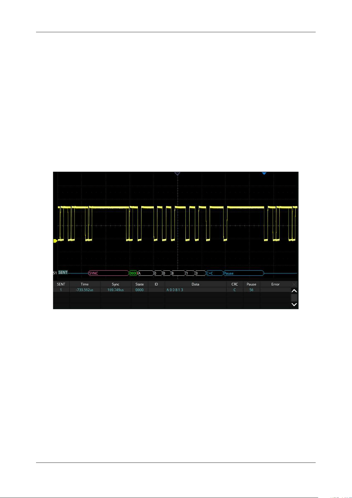
SDS6000L User Manual
1 5 0 i n t . s i g l e n t . c o m
14.11.3 SENT Serial Decode
The configuration of SENT decoding is similar to that of I2C decoding.
On the bus:
For Fast Channel:
SYNC is displayed in pink
STATE is displayed in green
DATA is displayed in white
CRC and Pause pulse are displayed in blue
For Slow Channel:
ID is displayed in green
DATA are displayed in white
CRC is displayed in blue
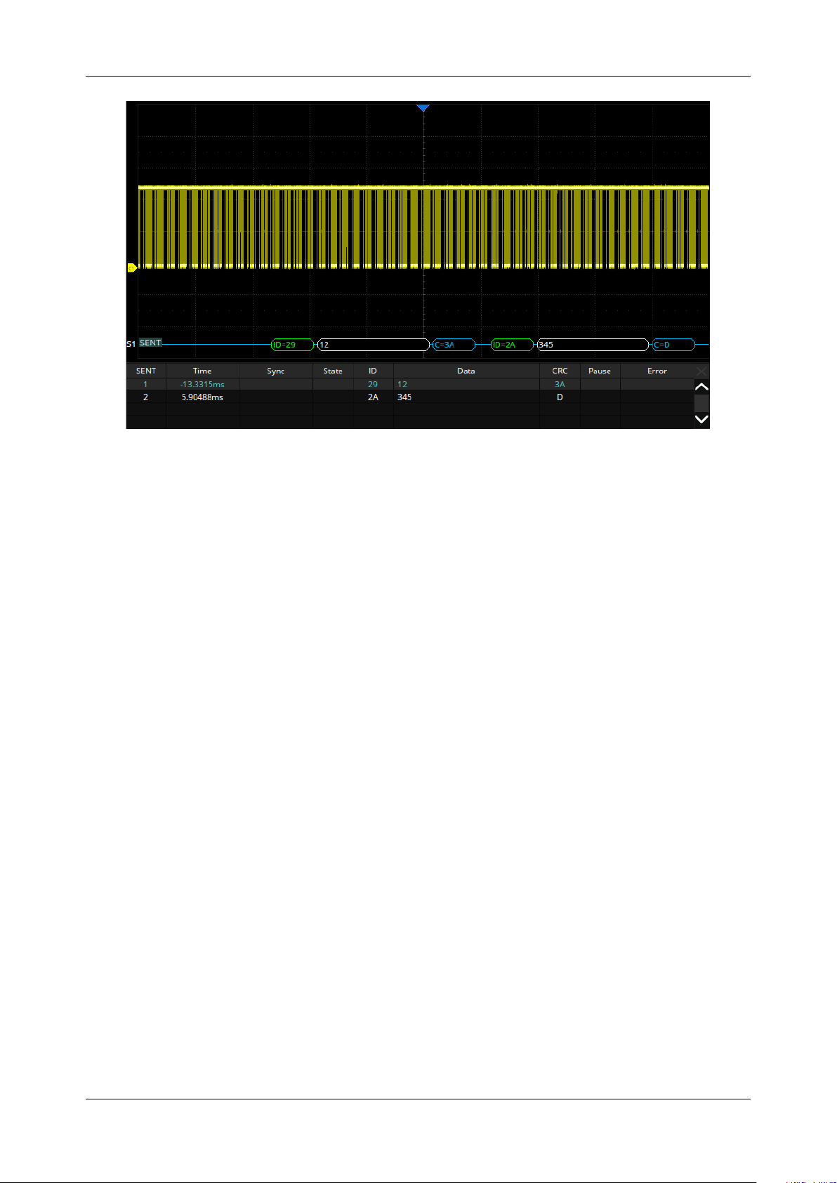
SDS6000L User Manual
int. s i g l e n t . c o m 1 5 1
In the list view:
Time — The horizontal offset of the current data frame head relative to the trigger position.
Sync — Sync pulse width (only fast channel)
State — Status & Communication nibble (only fast channel)
ID — ID of the frame (only slow channel).
Data — Data values
CRC — Cycle redundancy check
Pause — Pause ticks
Error — Error type
14.12 Manchester Serial Decode
This section covers decoding Manchester signals. Please read the following for more details:
"Manchester Signal Settings" and "Manchester Serial Decode".
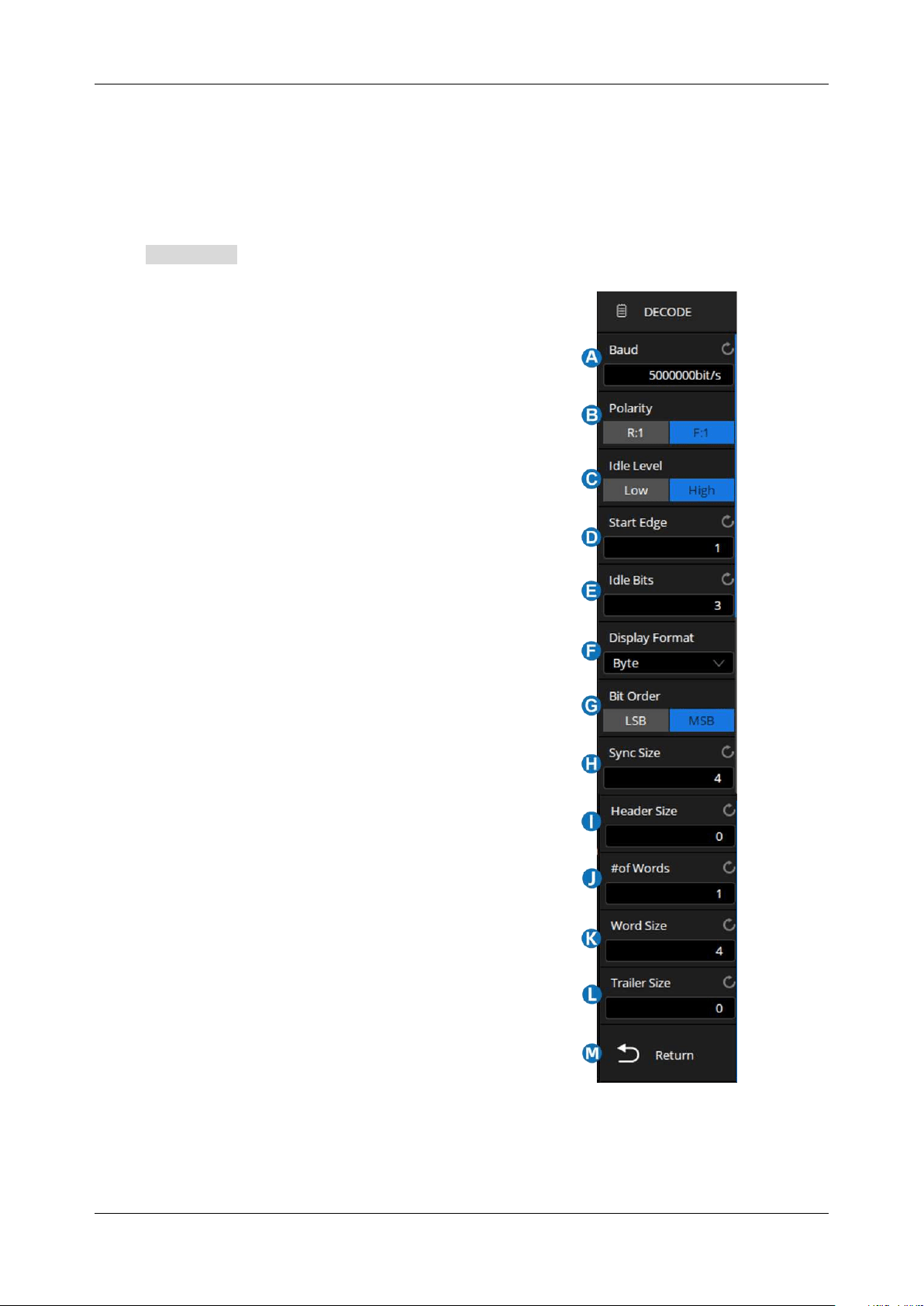
SDS6000L User Manual
1 5 2 i n t . s i g l e n t . c o m
14.12.1 Manchester Signal Settings
Connect the Manchester signal to the oscilloscope, set the mapping relation between channels and
signals, and then set the threshold level of the signal. The process of specifying the source and
threshold is similar to "I2C Signal Settings"
In the BusConfig menu of decode, the following parameters are available:
A. Click to specify the baud rate, the range is 500
b/s to 5 Mb/s
B. Set the Manchester signal's logic type. R:1
indicates that the rising edge is used to encode
a bit value of logic 1, and F:1 indicates that the
falling edge is used to encode a bit value of
logic 1
C. Set the idle level
D. Set the starting edge of the Manchester signal.
The range is 1~32
E. Set the minimum idle time/inter-frame gap time
of the Manchester bus in terms of the bit width.
F. Set the display format to Byte or Bit
G. Set the bit order to MSB or LSB
H. Set the sync field size, from 0 to 32
I. Set the header size, from 0 to 32
J. Set the number of words in the data field, from
1 to 255
K. Set the data word size, from 2 to 8
L. Set the trailer size, from 0 to 32
M. Return to the previous menu
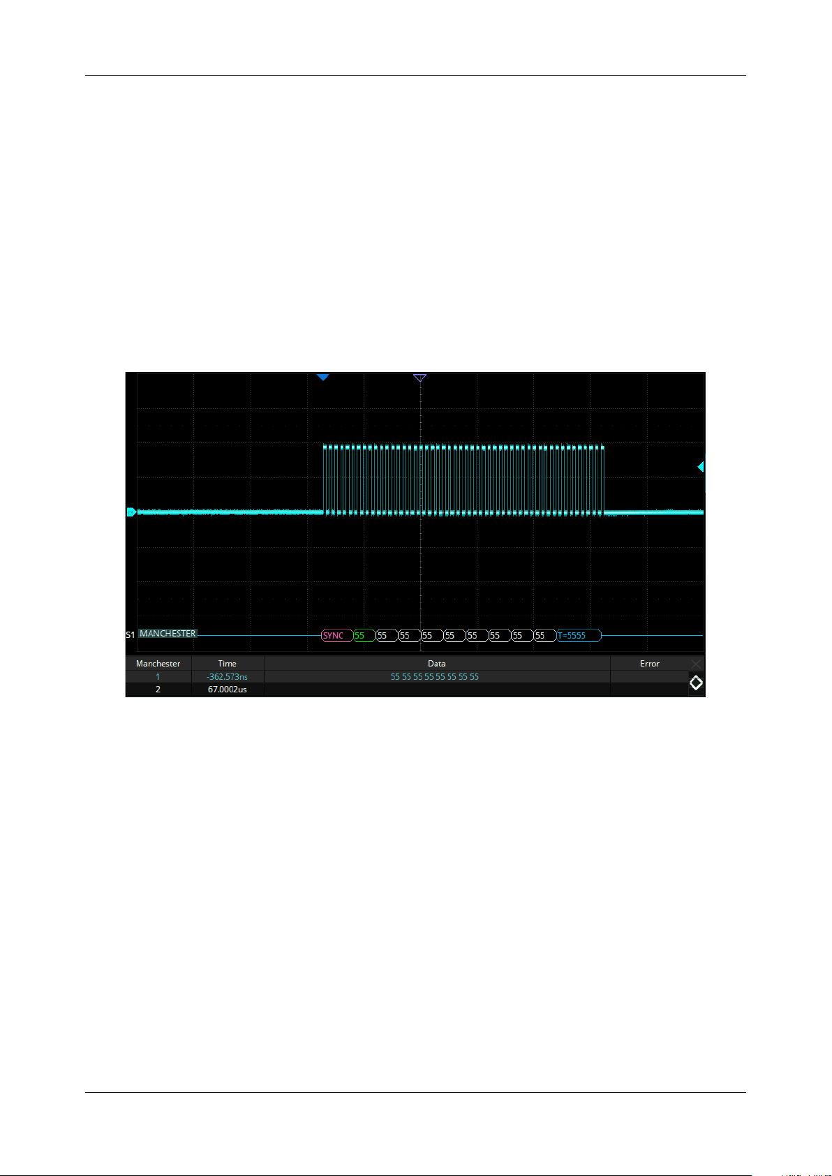
SDS6000L User Manual
int. s i g l e n t . c o m 1 5 3
14.12.2 Manchester Serial Decode
The configuration of Manchester decoding is similar to that of I2C decoding.
On the bus:
SYNC is displayed in pink
The header is displayed in green
DATA is displayed in white
The trailer is displayed in blue
In the list view:
Time -- The horizontal offset of the current data frame head relative to the trigger position.
Data -- Data words
Error -- Error type
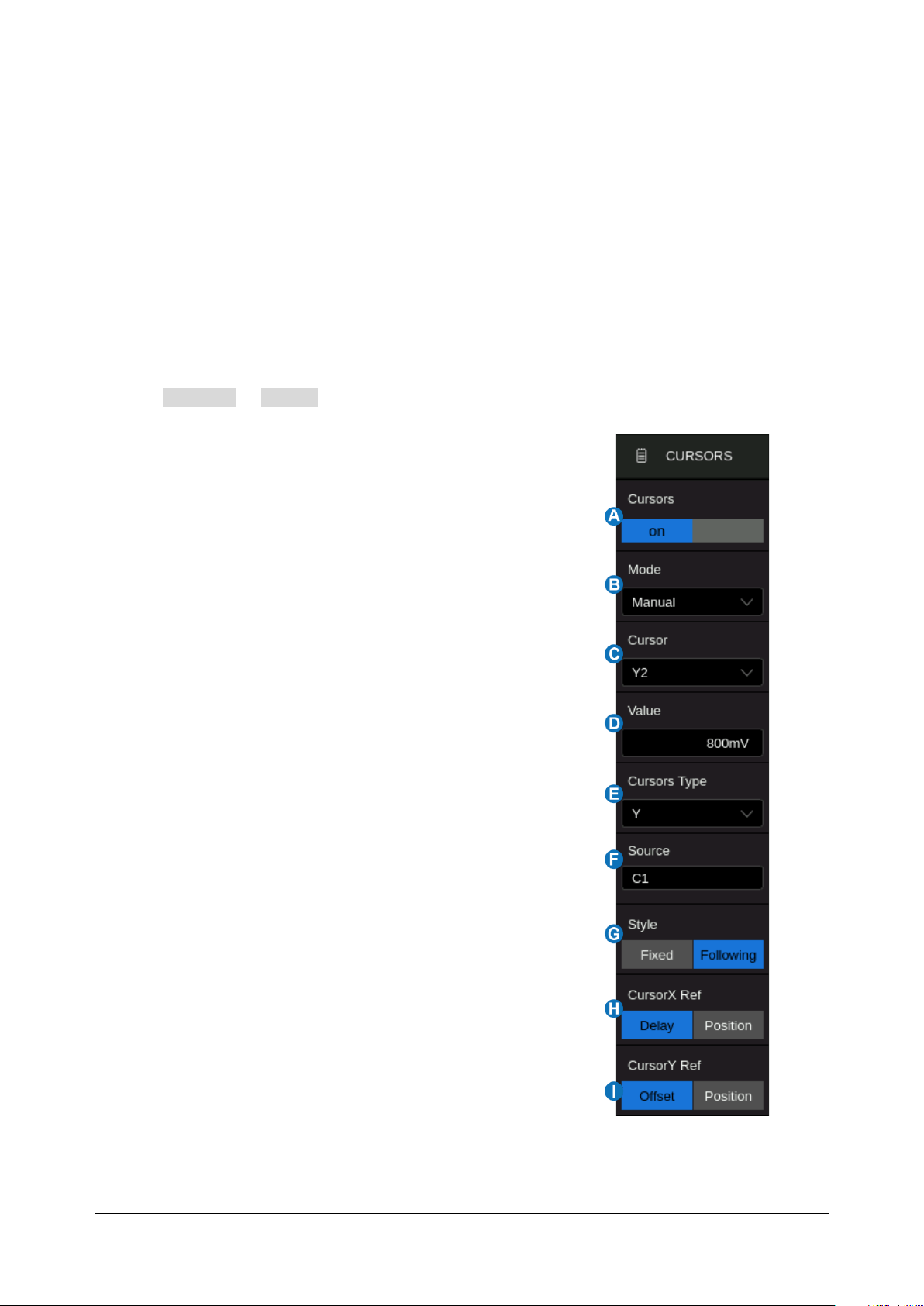
SDS6000L User Manual
1 5 4 i n t . s i g l e n t . c o m
15 Cursors
15.1 Overview
Cursors are important tools when measuring signals. Rapid measurements can be performed using
cursors in both horizontal and vertical directions. The cursor types include X1, X2, X1-X2, Y1, Y2, and
Y1-Y2, used to indicate X-axis values (time or frequency) and Y-axis values (amplitude) on a selected
waveform (C1~C8/F1~F4/M1~M4/REF/Histogram).
Perform Cursors > Menu to open the cursors dialog box:
A. Turn the cursor function on or off
B. Cursor Mode. The vertical cursors will automatically
track the waveform in Trace mode.
C. Specify the cursor
D. Set the position of the specified cursor
E. Select the cursors type (horizontal, vertical, horizontal +
vertical), this option is supported only in "Manual" mode.
F. Select the source
G. Display style of cursors text
H. X cursor reference (Delay or Position)
Delay measures the cursor position relative to the
Horizontal Delay/Offset position
Position measures the cursor position relative to the
horizontal center of the display
I. Y cursor reference (Offset or Position), this option is
supported only in "Manual" mode.
Offset measures the cursor position relative to the
Vertical/Offset position
Position measures the cursor position relative to the
vertical center of the display
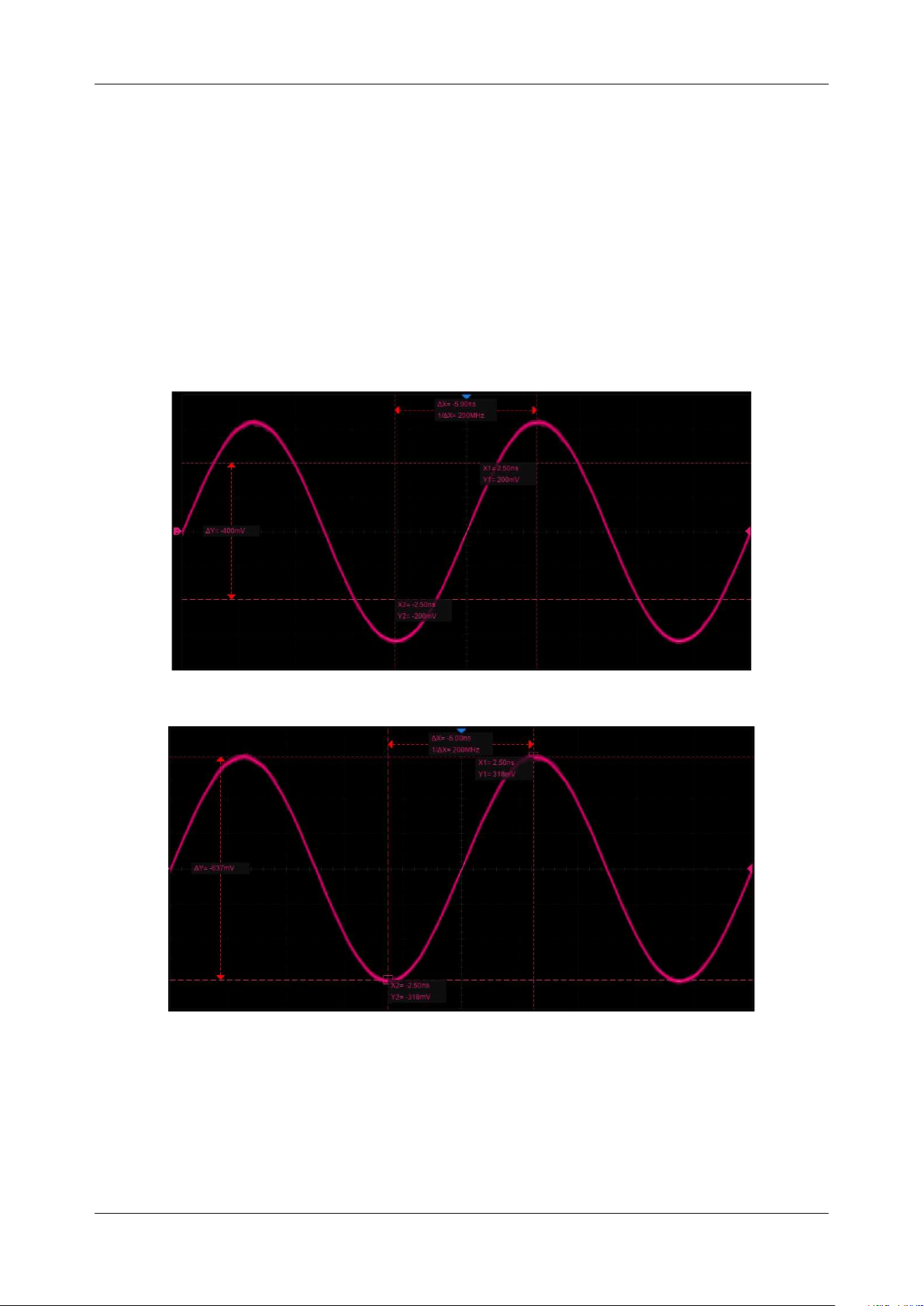
SDS6000L User Manual
int. s i g l e n t . c o m 1 5 5
Cursors Mode
Manual -- Manually sets the cursors’ position. Cursors type (horizontal, vertical, horizontal +
vertical) is available in this mode.
Track -- The cursor type is automatically set to "horizontal + vertical". In this mode, only horizontal
cursors are adjustable, while the vertical cursors automatically attach to the cross-point of the
cursor and the source waveform.
Measure – Automatically indicates the measured item using cursors
Manual Mode
Track Mode
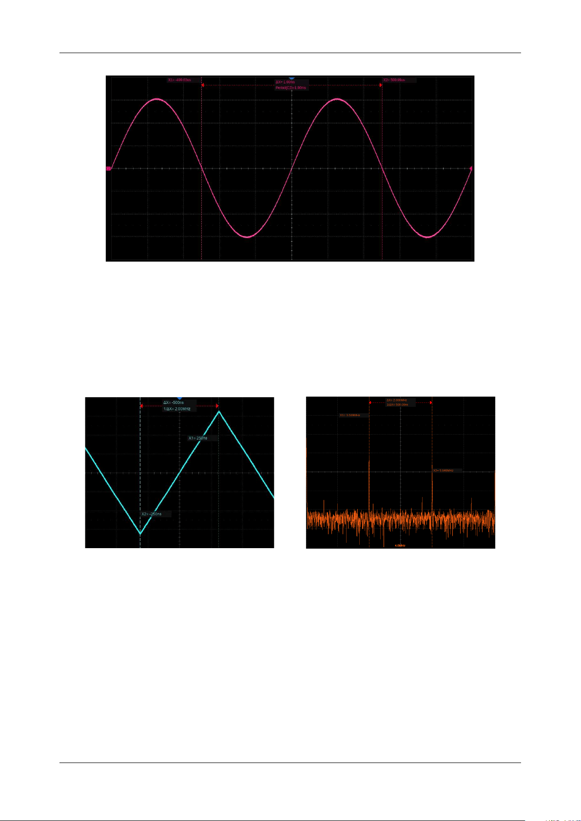
SDS6000L User Manual
1 5 6 i n t . s i g l e n t . c o m
Measure Mode
Cursors Type
X (horizontal) -- Vertical dotted lines that measure horizontal time (when the source is an FFT waveform,
X cursors measure frequency).
X cursors (time)
X cursors (frequency)
X1
-- The left (default) vertical dotted line. It can be manually moved to any horizontal position
on the screen.
X2
-- The right (default) vertical dotted line. It can be manually moved to any horizontal
position on the screen.
X1- X2
-- The difference between X1 and X2. After this option is selected, changing the value
will move both X1 and X2 simultaneously.
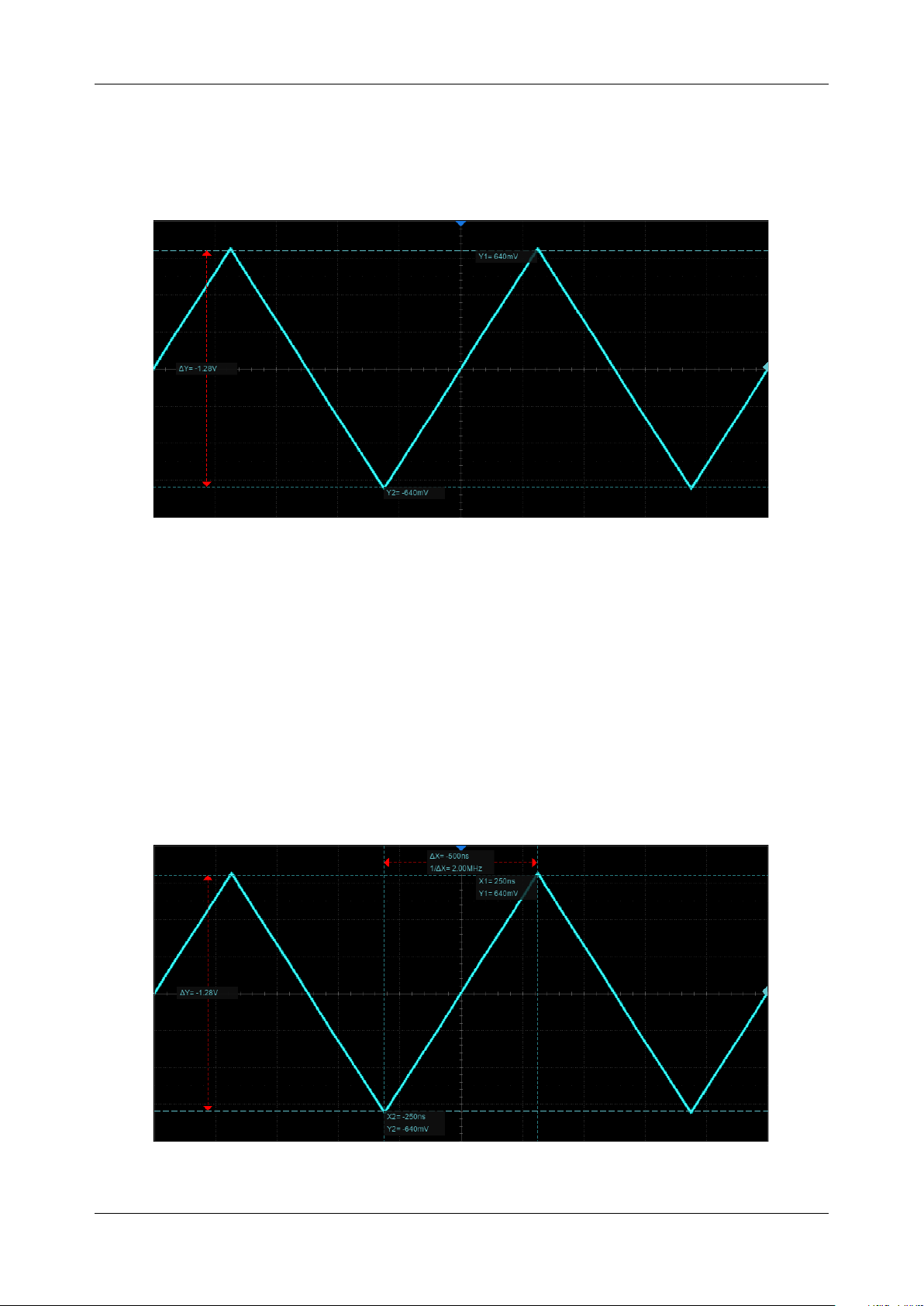
SDS6000L User Manual
int. s i g l e n t . c o m 1 5 7
Y
(
vertical
)
-- Horizontal dotted lines that measure vertical voltage or current (depending on the unit
of the selected channel). When the cursor's source is the math function, the units will match the math
function.
Y1
-- The upper (default) horizontal dotted line. It can be manually moved to any vertical
position on the screen.
Y2
-- The lower (default) horizontal dotted line. It can be manually moved to any vertical
position on the screen.
Y1- Y2
-- The difference between Y1 and Y2. After this option is selected. Change the value
to move both Y1 and Y2 simultaneously.
X+Y (horizontal + vertical) -- Both the X cursors and Y cursors are enabled.
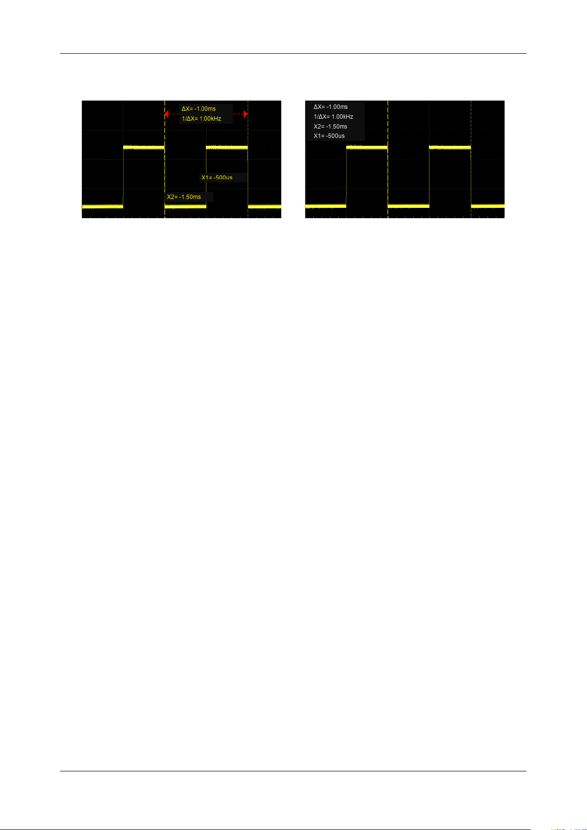
SDS6000L User Manual
1 5 8 i n t . s i g l e n t . c o m
Display Mode
Display Mode M1
Display Mode M2
M1 -- The position information of each cursor is attached to the cursor, and the difference
information is between the two cursors with arrows connected to the cursors. This mode is more
intuitive.
M2 -- The position information of each cursor and the difference between the cursors are displayed
in a region on the screen. The region can be moved by dragging to avoid covering the waveform.
This mode is relatively concise.
Cursors Reference
X cursors reference:
Fixed Delay– When the timebase is changed, the value of X cursors remains fixed.
Fixed Position– When the timebase is changed, the X cursors remain fixed to the grid position
on the display.
Y cursors reference:
Fixed Offset– When the vertical scale is changed, the value of
Y- cursors remain fixed.
Fixed Position– When the vertical scale is changed, the Y-cursors remain fixed to the grid
position on the display.
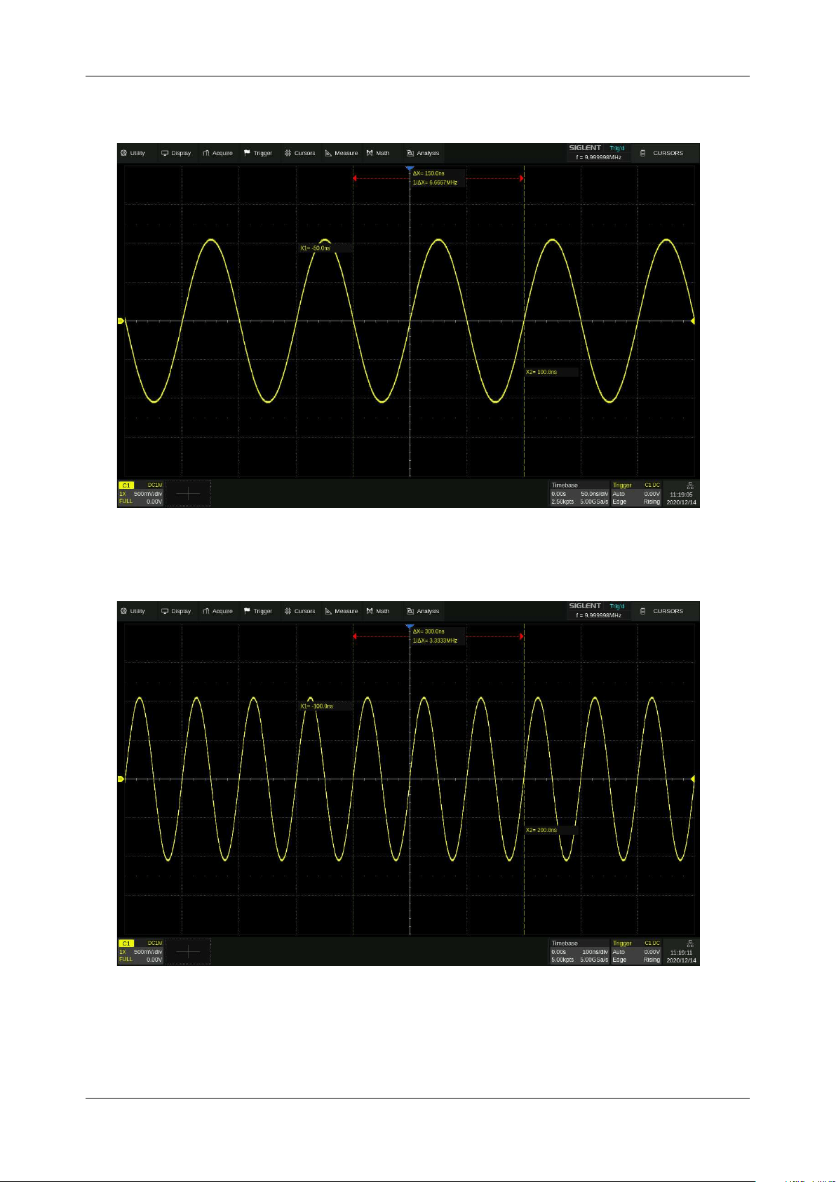
SDS6000L User Manual
int. s i g l e n t . c o m 1 5 9
Take the X cursors reference as an example to demonstrate the scaling effect of different settings:
Timebase=50ns/div
,
X1=-50ns=-1div
,
X2=100ns=2div
Fixed position, timebase is changed to 100 ns/div, and the grid number of X cursors
(-1div, 2div) remains fixed. The value of X1 and X2 is changed to -100 ns, 200 ns.
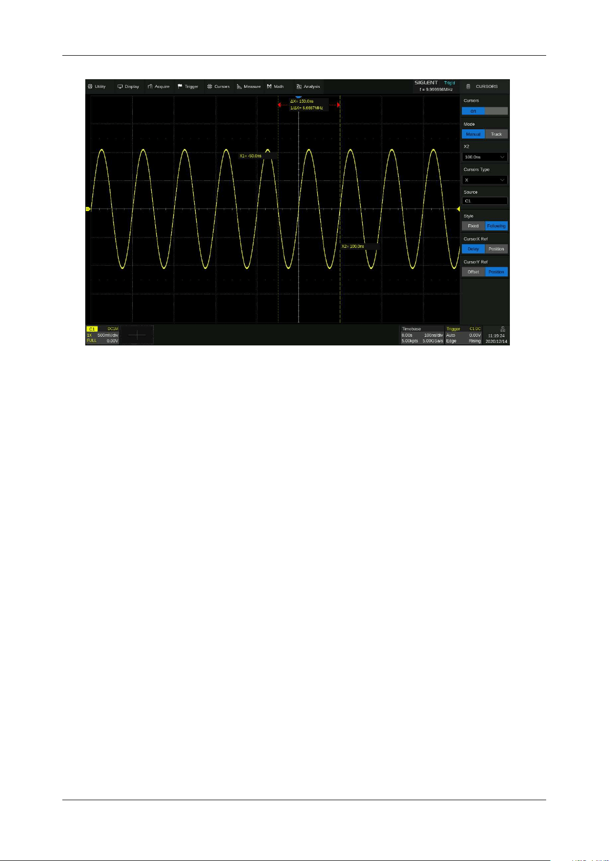
SDS6000L User Manual
1 6 0 i n t . s i g l e n t . c o m
Fixed delay, timebase is changed to 100 ns/div, and the value of X cursors (-50 ns, 100 ns)
remains fixed. The grid number of X cursors is changed to -0.5div, 1div.
15.2 Select and Move Cursors
The cursors can be selected and moved directly by the mouse, in addition, they can be selected in the
cursor’s value dialog box.
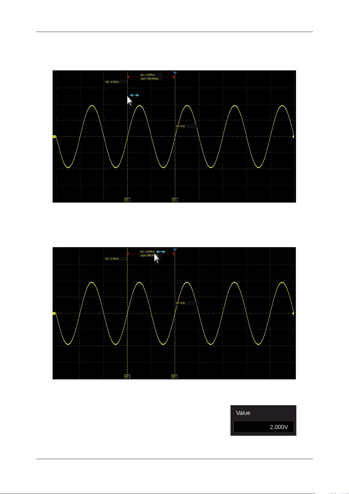
SDS6000L User Manual
int. s i g l e n t . c o m 1 6 1
Mouse
Directly click the cursor and drag it, as shown below:
Click the display area of
△
X (or
△
Y) in M1 mode and drag it to move the two cursors simultaneously,
as shown in the figure below. This is equivalent to the operation on the cursor type X1-X2 or Y1-Y2.
Dialog Box
Click the cursor value area of the dialog box, and then roll the
mouse wheel to adjust the position.
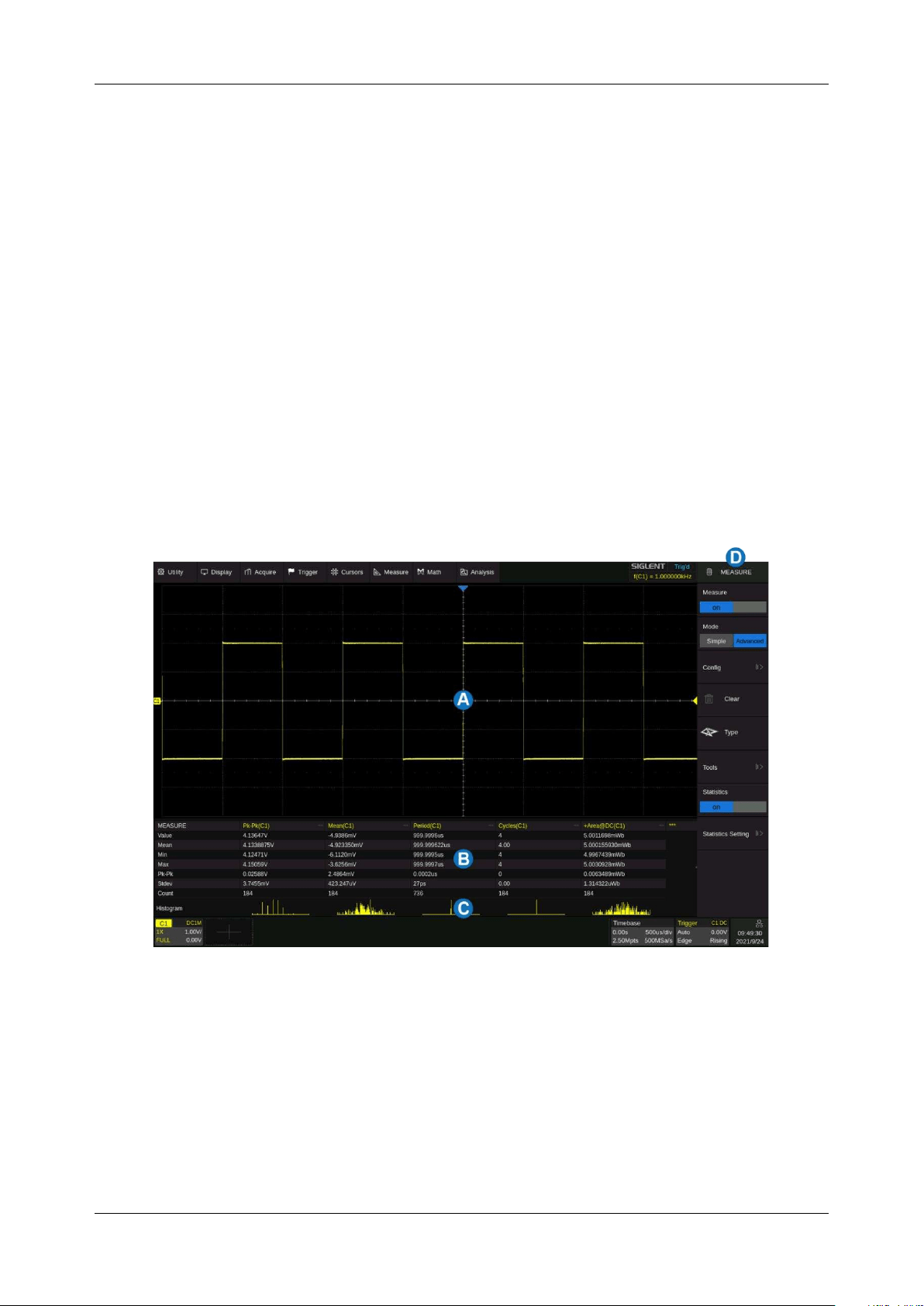
SDS6000L User Manual
1 6 2 i n t . s i g l e n t . c o m
16 Measurement
16.1 Overview
The SDS6000L features a strong automatic measurement list. These parameters can be automatically
measured without cursors and include common measurements such as rise time, fall time, peak-peak,
and period. The SDS6000L can also measure multiple channels at the same time, showing up to 6
parameter measurements with statistics while in the M1 display mode and up to 12 parameters in the
M2 mode. If you wish to view more parameters on a specified channel, then the "Simple" mode can be
employed. For measuring waveform of interest in a time gate, the "Gate" function is suggested.
Some parameter measurements (such as the mean) may be a value generated by all the data in a
frame. Some parameter measurements (such as period) accumulate all measurements in a frame, but
the displayed value is always the first value. If you want to know the distribution of multiple parameters
in one frame, you should use the statistics function.
A. The waveform display area automatically compresses when the other windows are displayed
B. Measurement parameters and statistics display area. If select the mode as “Simple”, the "Simple"
parameter area is displayed
C. Statistics histogram display area
D. Measure dialog box
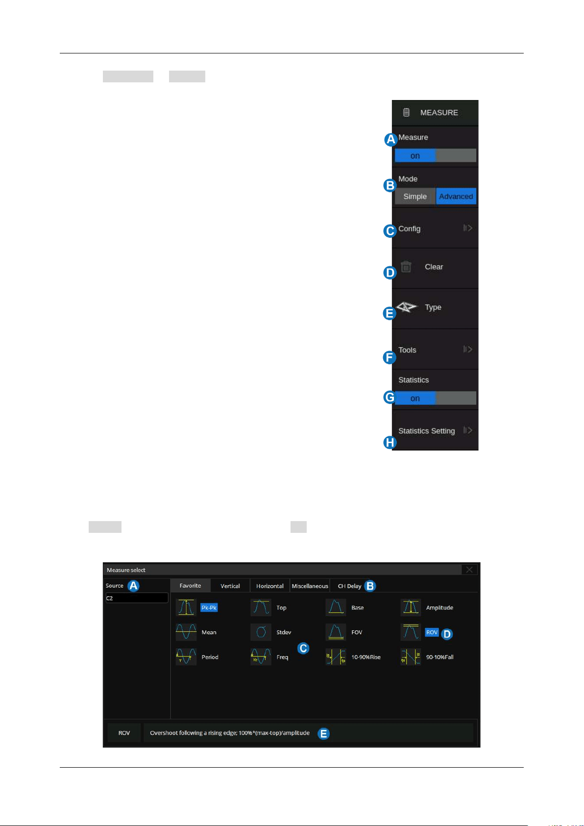
SDS6000L User Manual
int. s i g l e n t . c o m 1 6 3
Perform Measure > Menu to open the dialog box.
A. Enable/disable measure
B. Set the mode of measure: Simple or Advanced.
"Simple" shows the specified basic measurement
parameters of the selected channel. In "Advanced"
mode, the measurement parameters can be added
one by one as needed
C. Measure configuration: gate, amplitude strategy,
threshold, and display mode
D. Clear all the selected measurements
E. Select measurement parameters
F. Tools including Trend, Track, and Measure Cursor
G. Turn on or off statistics
H. Statistics settings: count limit, reset statistics, and
histogram
16.2 Set Parameters
Click Type in the measure dialog box, or click + in the measurement parameters and statistics
display area to open the parameter selection window:
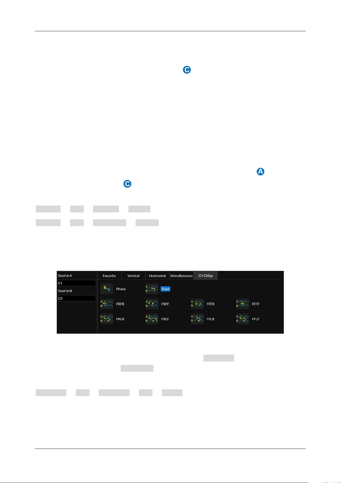
SDS6000L User Manual
1 6 4 i n t . s i g l e n t . c o m
A. Set the source of the current setting.
B. Measurement parameter classification tabs, including Favorite, Vertical, Horizontal,
Miscellaneous, and CH Delay. Click a tab and the area will display the corresponding
parameters
C. Parameters. Click the parameter to be measured to activate it, and click it again to close the
parameter.
D. Background highlighted parameters represent it is activated. In the figure above, "Pk-Pk" and
"ROV" are activated.
E. Description of the last selected parameter.
The correct steps to add a measurement parameter are to select the source in the area and
then select the parameter in the area. For example, to add Pk-Pk measurements for C1 and
Period measurements for C2, follow the steps below:
Source > C1 > Vertical > Pk-Pk
Source > C2 > Horizontal > Period
For the channel delay (CH Delay) measurement, because the number of sources involved is greater
than 1, the steps to specify the source are different:
In the parameter selection area, the channel corresponding to Source A is specified first, and then
the channel corresponding to Source B . Finally, the measurement parameter is selected. For
example, to activate the skew between C1 and C2, you can follow the following steps:
Source A > C1 > Source B > C2 > Skew
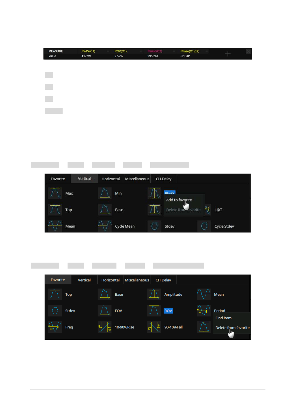
SDS6000L User Manual
int. s i g l e n t . c o m 1 6 5
Once a parameter is selected, it will appear in the parameter and statistical display area below the grid:
Click + in the blank area to add a parameter.
Click – in the upper right corner of each parameter to close the parameter.
Click × in the upper right corner of the area to close the measurement.
Click Clear in the dialog box to close all parameters.
The “Favorite” tab is used to store frequently used items. You can customize this tab. Up to 20 items
can be stored in it. Long-click an item to add or remove it from the “Favorite” tab. For example, to add
Pk-Pk to the “Favorite” tab:
Advanced > Type > Vertical > Pk-Pk > Add to favorite
To remove Period from the “Favorite” tab:
Advanced > Type > Favorite > Period > Delete from favorite
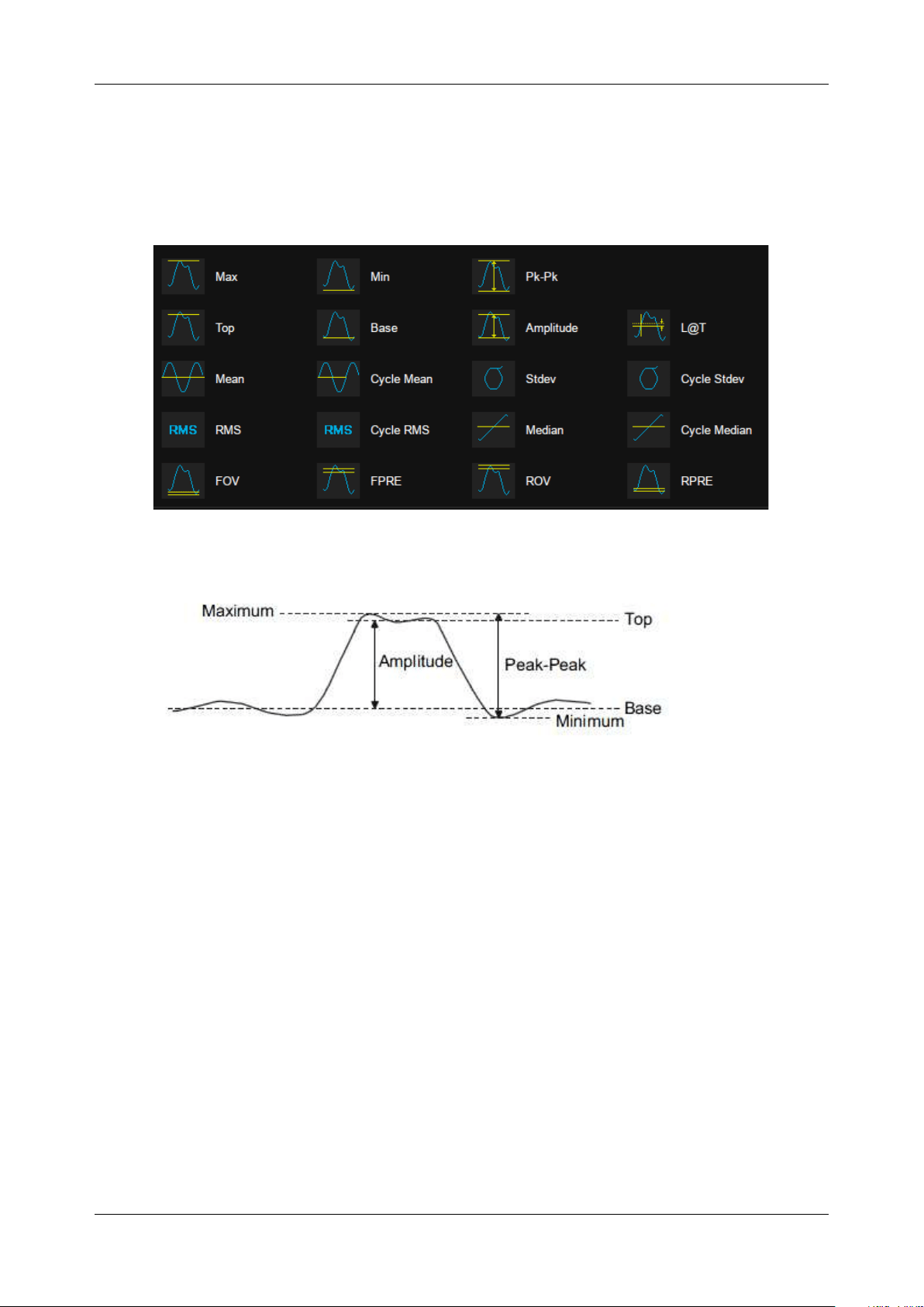
SDS6000L User Manual
1 6 6 i n t . s i g l e n t . c o m
16.3 Type of Measurement
16.3.1 Vertical Measurement
Vertical measurement includes 19 parameters:
Max:
Highest value in the input waveform
Min:
Lowest value in the input waveform
Pk-Pk:
Difference between maximum and minimum data values
Top:
Value of most probable higher state in a bimodal waveform
Base:
Value of most probable lower state in a bimodal waveform
Amplitude:
Difference between top and base in a bimodal waveform. If not bimodal, the
difference between max and min
Mean:
Average of data values
Cycle Mean:
Average of data values in the first cycle
Stdev:
Standard deviation of the data
Cycle Stdev:
Standard deviation of the data in the first cycle
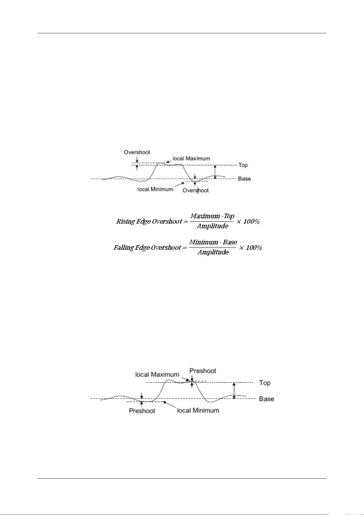
SDS6000L User Manual
int. s i g l e n t . c o m 1 6 7
RMS:
Root mean square of the data
Cycle RMS:
Root mean square of the data in the first cycle
Median:
Value at which 50% of the measurements are above and 50% are below
Cycle Median:
Median of the first cycle
Overshoot (FOV):
Overshoot following a falling edge; 100%* (base-min)/amplitude
Overshoot (ROV):
Overshoot following a rising edge; 100%*(max-top)/amplitude
Preshoot (FPRE):
Overshoot before a falling edge.
Equal to 100 %*( max-top)/amplitude.
Preshoot (RPRE):
Overshoot before a rising edge.
Equal to 100 %*( base-min)/amplitude.
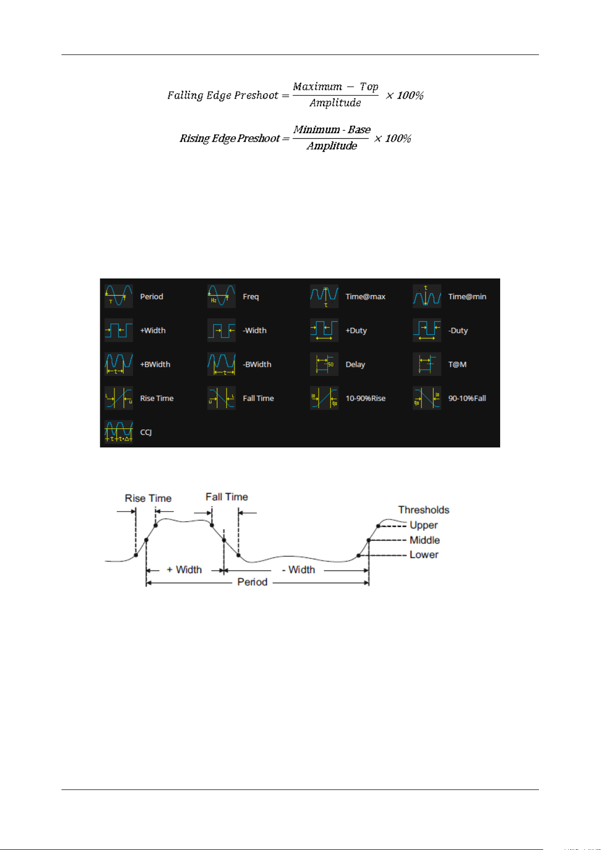
SDS6000L User Manual
1 6 8 i n t . s i g l e n t . c o m
L@T:
Level measured at trigger position
16.3.2 Horizontal Measurement
Horizontal measurement includes 17 parameters:
Period:
Time between the middle threshold points of two consecutive like-polarity edges.
Freq:
Reciprocal of the period
Time@max:
First time of maximum value
Time@min:
First time of minimum value
+Width:
Time difference between the middle threshold of a rising edge to the middle
threshold of the next falling edge of the pulse
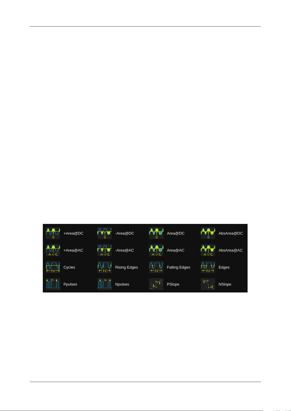
SDS6000L User Manual
int. s i g l e n t . c o m 1 6 9
-Width:
Time difference between the middle threshold of a falling edge to the middle
threshold of the next rising edge of the pulse
+Duty:
Positive Duty Cycle. The ratio of positive width to period
-Duty:
Negative Duty Cycle. The ratio of negative width to period
+BWidth:
Time from the first rising edge to the last falling edge at the middle threshold
-BWidth:
Time from the first falling edge to the last rising edge at the middle threshold
Delay:
Time from the trigger to the first transition at the middle threshold
T@M:
Time from the trigger to each rising edge at the middle threshold
Rise Time:
Duration of rising edge from lower threshold to upper threshold
Fall Time:
Duration of falling edge from upper threshold to lower threshold
10-90%Rise:
Duration of rising edge from 10-90%
90-10%Fall:
Duration of falling edge from 90-10%
CCJ:
The difference between two continuous periods
16.3.3 Miscellaneous Measurements
The Miscellaneous measurements tab includes 16 parameters:
+Area@DC:
Area of the waveform above zero
-Area@DC:
Area of the waveform below zero
Area@DC:
Area of the waveform
AbsArea@DC:
Absolute area of the waveform
+Area@AC:
Area of the waveform above average
-Area@AC:
Area of the waveform below average
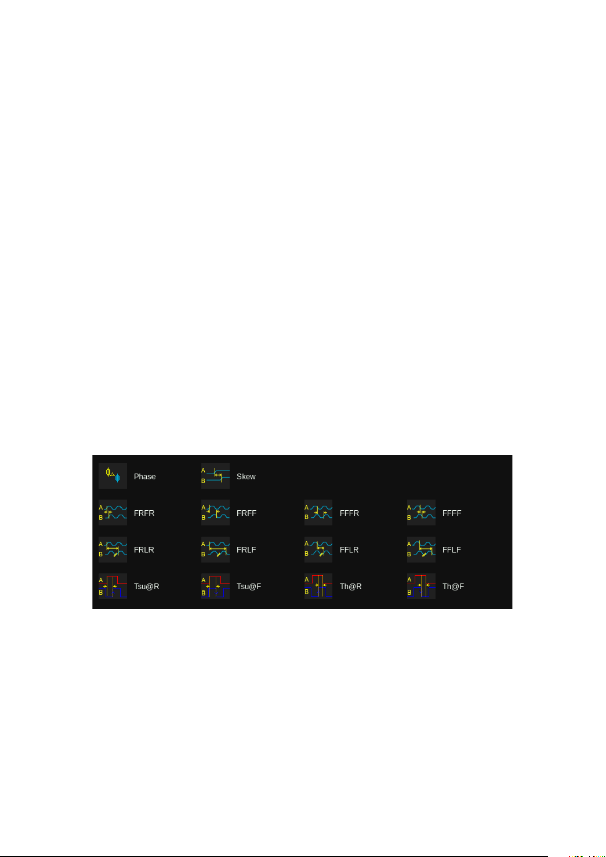
SDS6000L User Manual
1 7 0 i n t . s i g l e n t . c o m
Area@AC:
Area of the waveform above the average minus the area of the waveform
below average
AbsArea@AC:
Area of the waveform above the average plus the area of the waveform
below the average
Cycles:
Number of cycles in a periodic waveform
Rising Edges:
Number of rising edges in a waveform
Falling Edges:
Number of falling edges in a waveform
Edges:
Number of edges in a waveform
Ppulses:
Number of positive pulses in a waveform
Npulses:
Number of negative pulses in a waveform
PSlope:
The slope of the rising edge
NSlope:
The slope of the falling edge
16.3.4 Delay Measurement
Delay measurement measures the time difference between two channels. It includes 14 delay
parameters:
Phase:
Phase difference between two edges
Skew:
Time of source A edge minus time of nearest source B edge
FRFR:
The time between the first rising edge of source A and the following first rising
edge of source B at the middle threshold
FRFF:
The time between the first rising edge of source A and the following first falling
edge of source B at the middle threshold
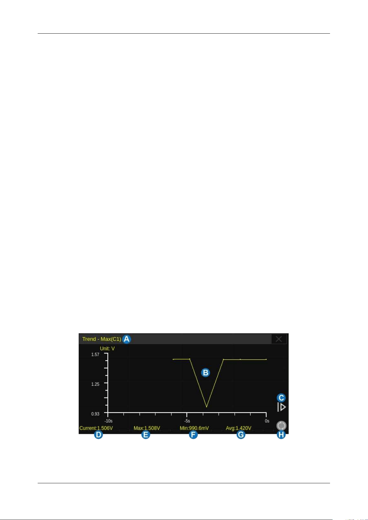
SDS6000L User Manual
int. s i g l e n t . c o m 1 7 1
FFFR:
The time between the first falling edge of source A and the following first rising
edge of source B at the middle threshold
FFFF:
The time between the first falling edge of source A and the following first falling
edge of source B at the middle threshold
FRLR:
The time between the first rising edge of source A and the last rising edge of
source B at the middle threshold
FRLF:
The time between the first rising edge of source A and the last falling edge of
source B at the middle threshold
FFLR:
The time between the first falling edge of source A and the last rising edge of
source B at the middle threshold
FFLF:
The time between the first falling edge of source A and the last falling edge of
source B at the middle threshold
Tsu@R:
Data setup time before the clock rising edge
Tsu@F:
Data setup time before the clock falling edge
Th@R:
Data hold time after the clock rising edge
Th@F:
Data hold time after the clock falling edge
16.4 Trend
After adding a measurement parameter, a Trend can be used to observe the long-term change of the
selected measurement value over time.
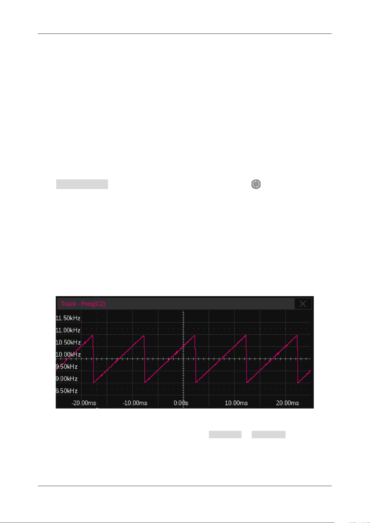
SDS6000L User Manual
1 7 2 i n t . s i g l e n t . c o m
A. Measurement parameter display area
B. Trend plot display area
C. Extend the range of time. Click it to expand the time range.
D. Current value
E. Maximum value
F. Minimum value
G. Average value
H. Reset statistics
Click Reset Statistics in the measure dialog box, or click the symbol in the statistics display
area to clear and restart statistics.
16.5 Track
The measure values VS. time plot of a horizontal parameter (e.g. frequency, rise time) in one frame
can be observed when the Track is enabled.
The upper limit of the statistic number in a frame is set in Statistics > AIM Limit , which means
the values exceeding the limit will not be shown in the track plot. The upper limit is 1,000 by default
and can be set to up to 65,000.
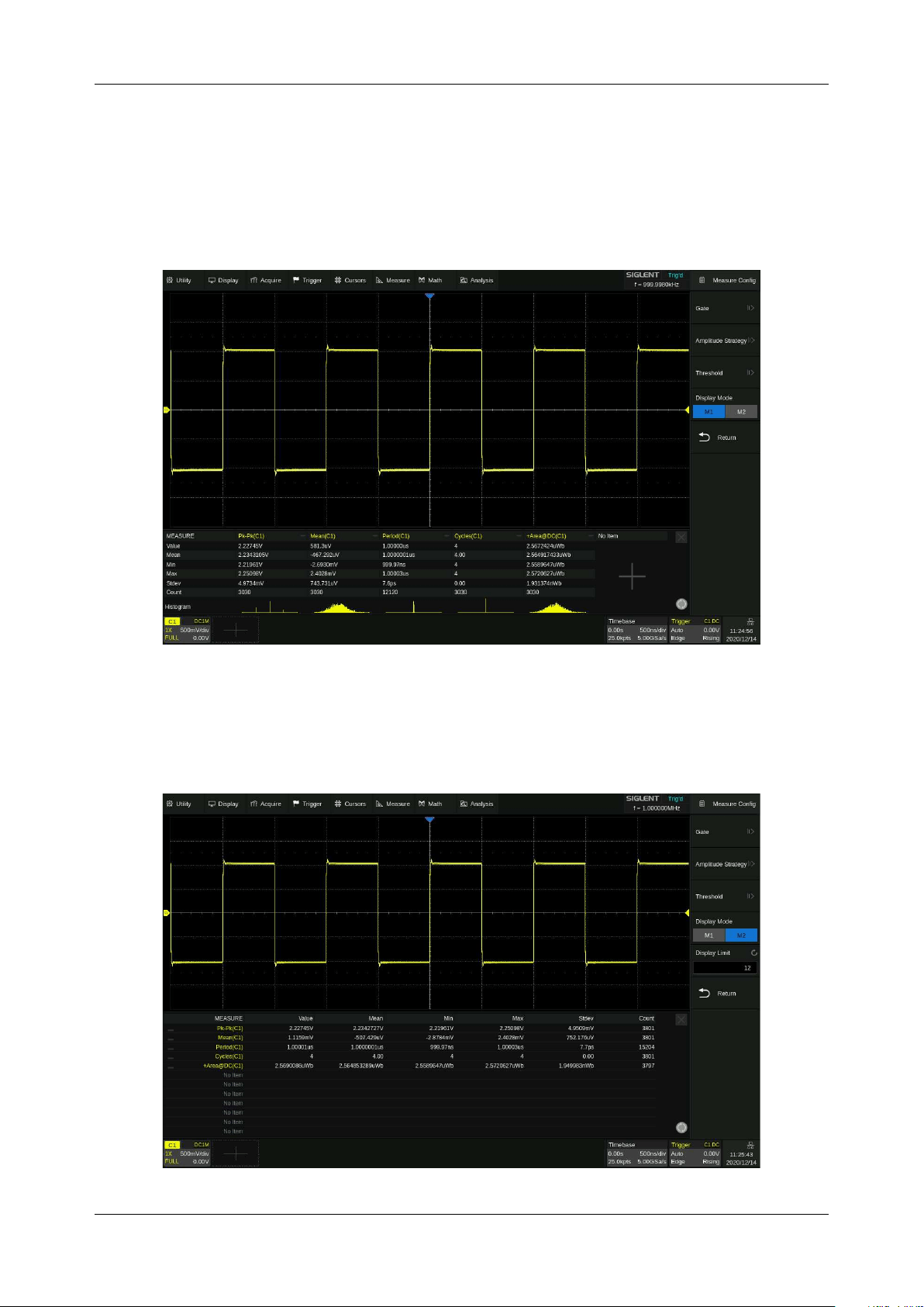
SDS6000L User Manual
int. s i g l e n t . c o m 1 7 3
16.6 Display Mode
In advanced measurement mode, two display modes are supported: M1 and M2.
In M1 mode, up to 6 parameter measurements are displayed at a time. When statistics are enabled,
they are listed under the measurement items. Click a column to add or replace a measurement.
In M2 mode, up to 12 parameter measurements are displayed at a time. When statistics are enabled,
they are distributed on the right side of the measurement item. Click a row to add or replace a
measurement.
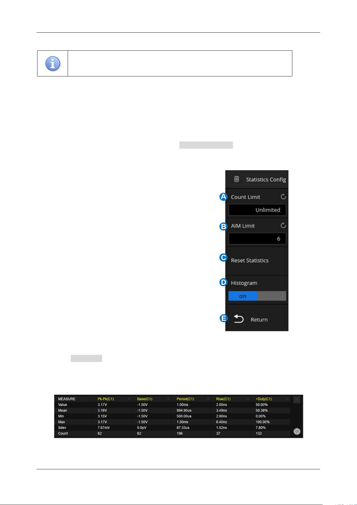
SDS6000L User Manual
1 7 4 i n t . s i g l e n t . c o m
Note:
In M2 mode histogram display is not supported.
16.7 Measurement Statistics
Measurement statistics are based on the total number of captured waveforms. In Roll mode,
measurement statistics increase over time. Click Statistics Setting in the measure dialog box to
recall the Statistics Config dialog box:
A. Set the maximum number of samples for the
statistics function. The setting range is 0 ~ 1024, or
unlimited. If there is no limit, the number of statistics
will be accumulated. If there is a limit, when the
maximum number of statistics N is reached, only the
latest N measurements will be counted. When the
count is limited, only the first period measurement
value of each frame is counted
B. Set the upper limit of the statistic number in a frame.
Valid only when the count limit is set to "Unlimited".
The setting range is 1 ~ 65,000
C. Clear and restart the statistics.
D. Turn the histogram on or off
E. Return to the previous menu
Enable the Statistics function to observe the distribution of the measured values of every selected
parameter.
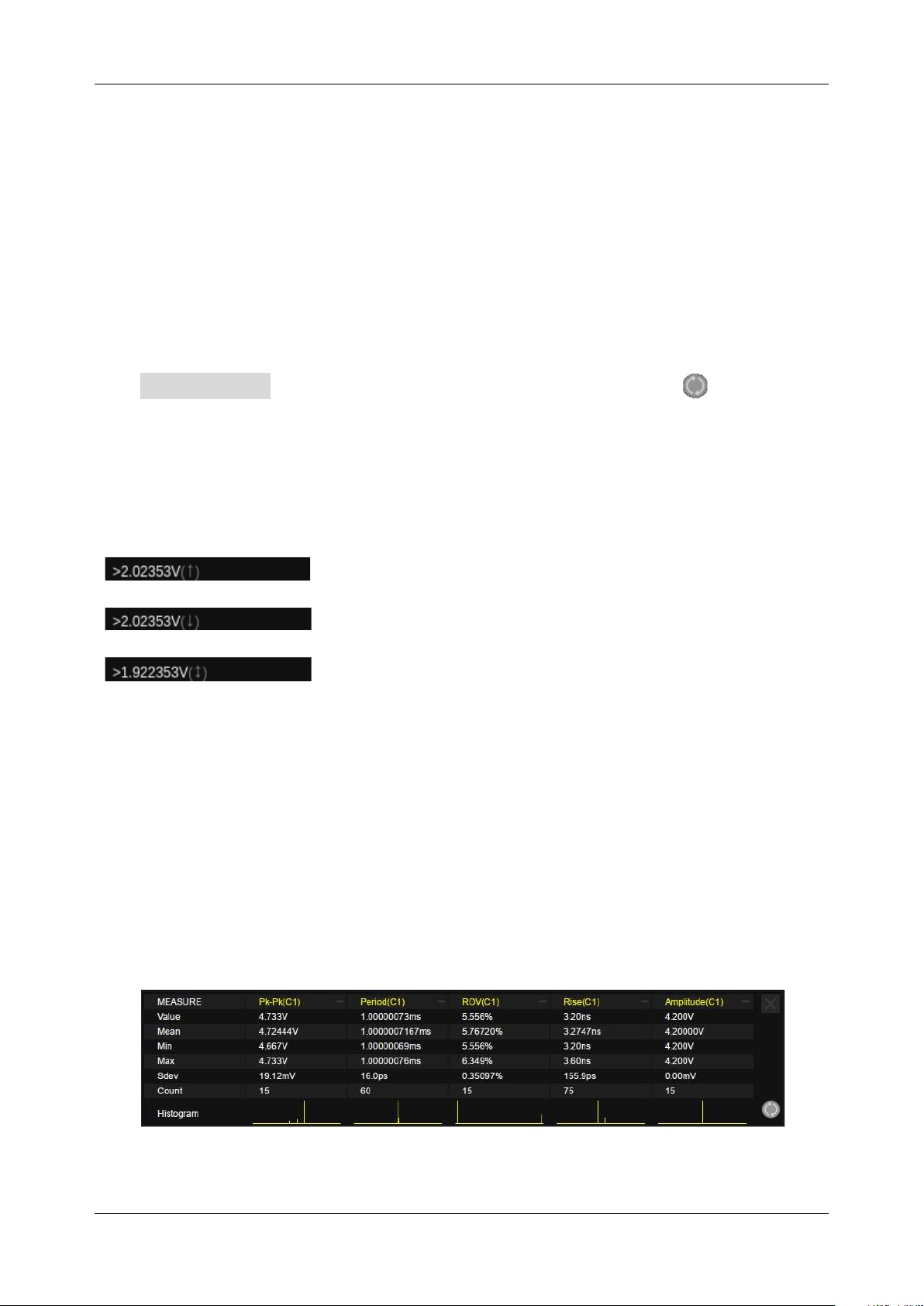
SDS6000L User Manual
int. s i g l e n t . c o m 1 7 5
Value –
The current measurement
Mean –
Average of all historical measurements
Min –
The minimum of all historical measurements
Max –
The maximum of all historical measurements
Stdev –
Standard deviation of all historical measurements
Count –
The number of historical measurements
Click Reset Statistics in the statistics setting dialog box, or click the symbol in the statistics
display area to clear and restart statistics.
When the oscilloscope detects the trace under test is clipped, an extra overflow indicator will appear
after the measurement value:
Waveform clipped at the top
Waveform clipped at the bottom
Waveform clipped at both top and bottom
16.8 Statistics Histogram
After enabling statistics on a selected measurement, you can also activate a statistical histogram. The
histogram appears at the bottom of the statistics area. This enables users to quickly view the probability
distribution of the measured parameters. The color of the histogram is consistent with the measurement
source (Channel 1 is yellow, etc.).
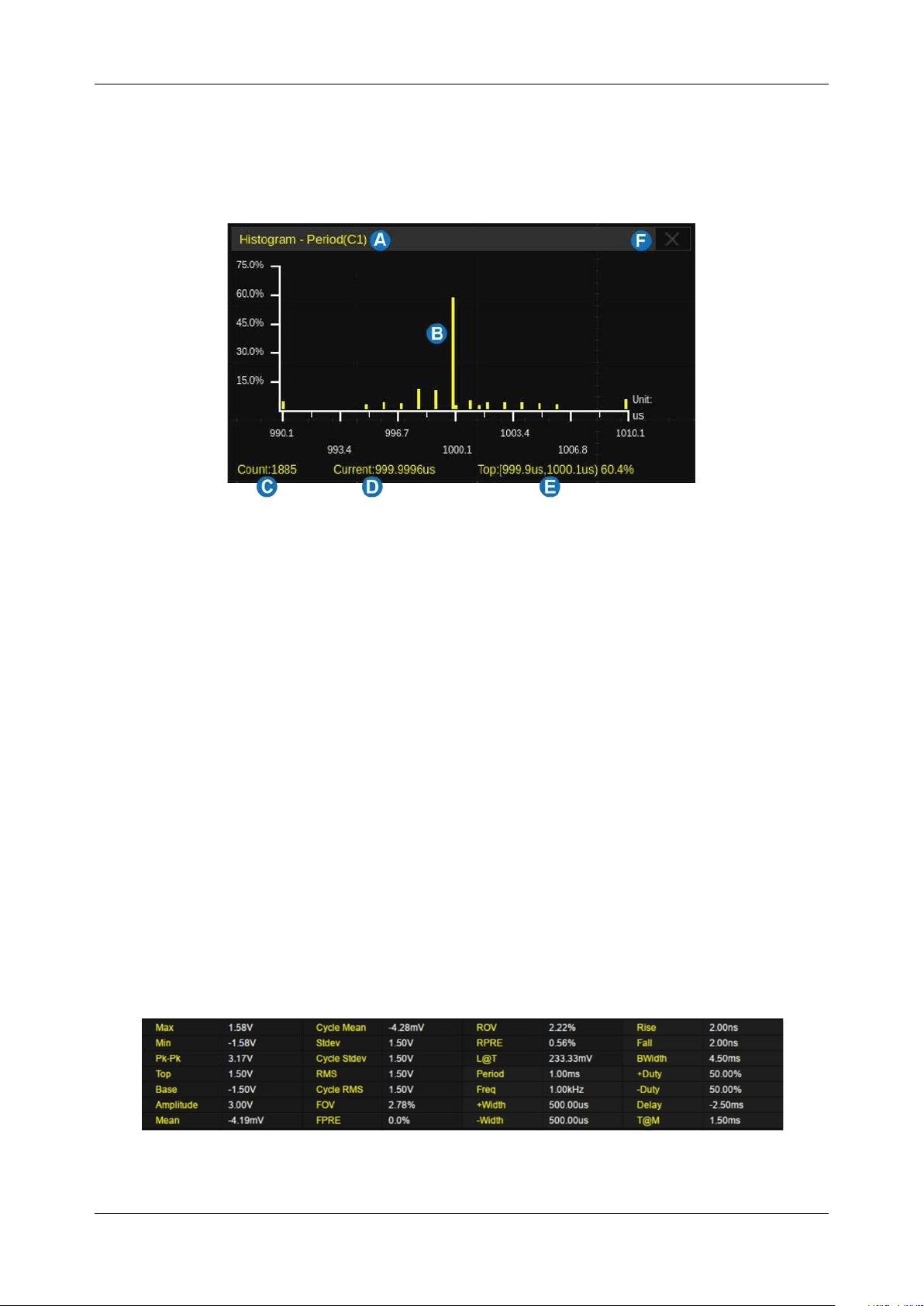
SDS6000L User Manual
1 7 6 i n t . s i g l e n t . c o m
Click the histogram area of a parameter to enlarge it for details. You can move the large histogram
window position around the display by dragging. Click the histogram of another parameter to switch to
the corresponding enlarged histogram.
A. Parameter
B. Histogram display area. The X-axis represents measured values and Y-axis represents the
probability.
C. Count of statistics
D. Current value
E. The bin that includes the maximum value and the probability of a value falling into it
F. Close the enlarged histogram
16.9 Simple Measurements
Enabling Simple Measurement displays all selected measurement parameters of the specified channel
at the same time. The font color of the measurement parameters is consistent with the color of the
specified source. Yellow for Channel 1, Purple for Channel 2, etc.
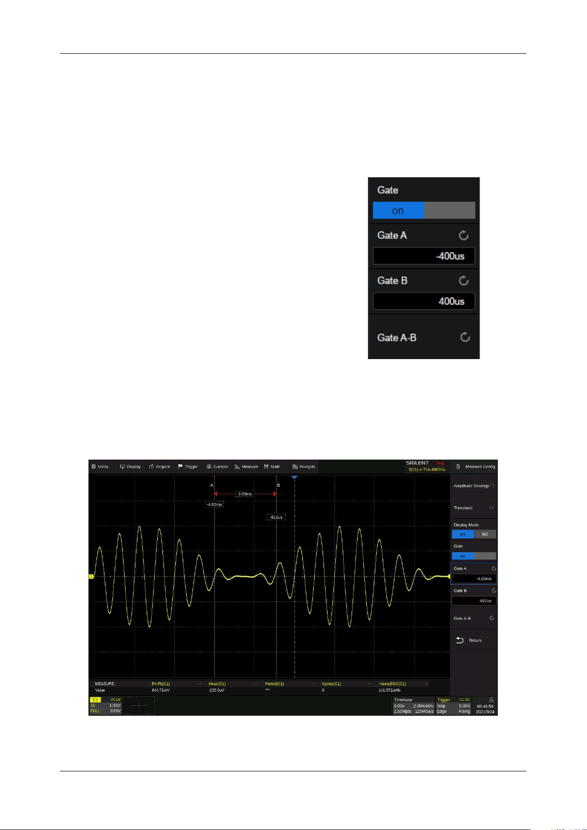
SDS6000L User Manual
int. s i g l e n t . c o m 1 7 7
16.10 Gate
Sometimes the user may want to measure parameters for a certain specified time range of the signal
and ignore signal parts that lie outside of that range. In this case, the Gate function can be helpful.
Turn on the Gate, then two horizontal cursors A and B will
appear in the grid area. The gate setting dialog box will be
displayed on the right.
Gate cursors A and B are used to define the range of time for
parameter measurements. The oscilloscope only measures
the parameters of the data between A and B, ignoring the
data outside the range.
The setting of gate cursors is similar to that of ordinary
cursors. See "Select and Move Cursors" for details.
The figure below shows a scenario in which the gate function is used to measure the peak-peak
parameter of the trough of an amplitude-modulated waveform:
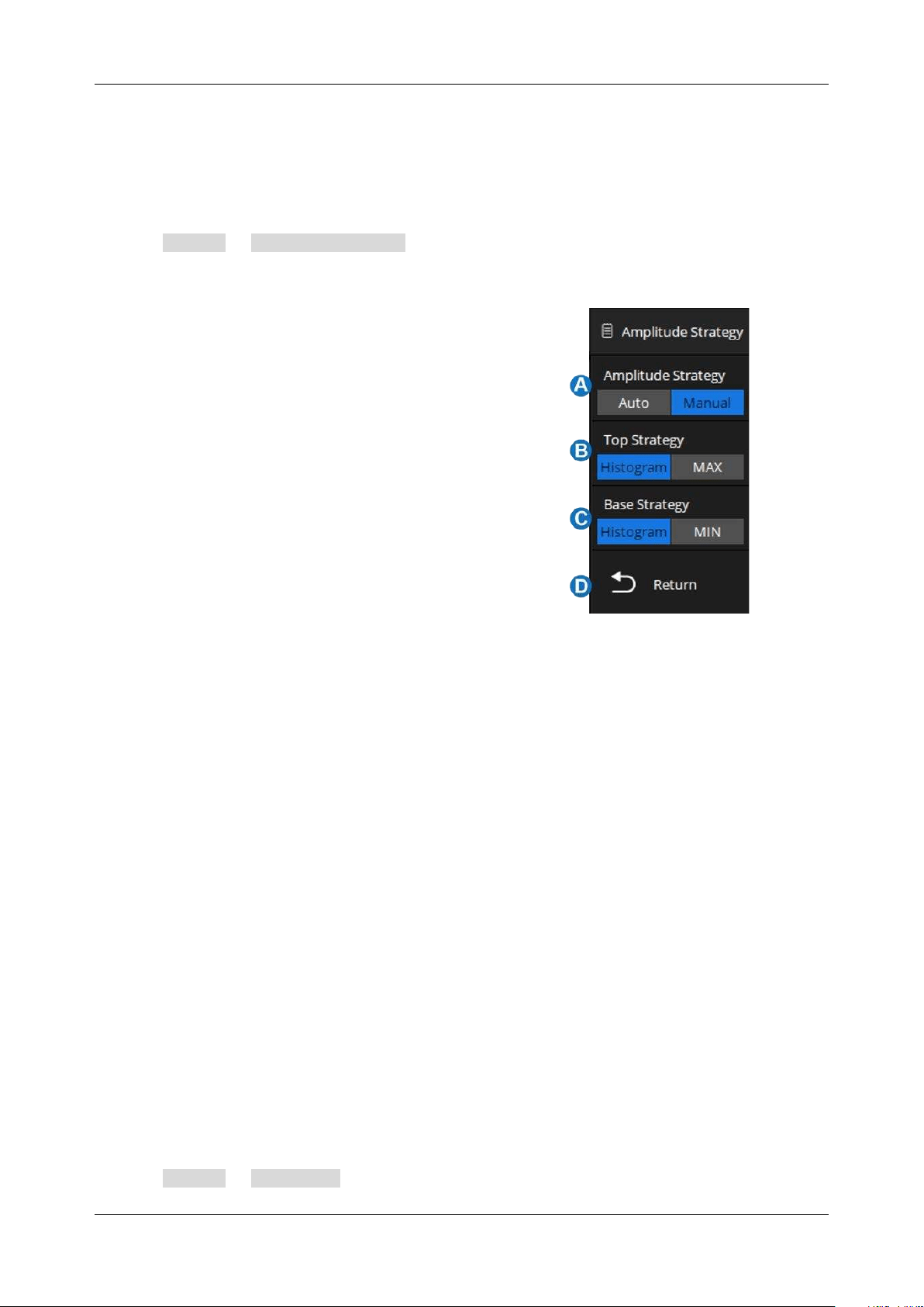
SDS6000L User Manual
1 7 8 i n t . s i g l e n t . c o m
16.11 Amplitude Strategy
According to different types of input signals, users can choose the corresponding amplitude calculation
strategy which can measure top and bottom values with more accuracy.
Perform Config > Amplitude Strategy in the measure dialog box to recall the amplitude strategy
dialog box:
A. Set the amplitude calculation strategy. When set
to Auto, the amplitude calculation strategy will be
selected automatically according to the input
signal to ensure the accuracy of the measured
value
B. Set the top value calculation strategy. When set
to Histogram, the value at the upper half of the
waveform will be counted, and the value with the
maximum probability will be identified as the top
value; when set to max, the maximum value of
the waveform will be identified as the top value
C. Set the base value calculation strategy. When set to Histogram, the value at the lower
half of the waveform will be counted, and the value with the maximum probability will be
identified as the base value; when set to min, the minimum value of the waveform will be
identified as the base value
D. Return to the previous menu
16.12 Threshold
Measurement thresholds can be defined by the user. This is more flexible than fixed thresholds. For
example, for pulse-width measurement, the threshold can be specified rather than fixed at 50%. For
rise time, the lower / upper thresholds can be specified rather than fixed at 10% / 90%.
Changing the default threshold may change the measurement results of relevant measurement items,
such as Period, frequency, +width, -width, +duty, -duty, +BWidth, -BWidth, delay, T@M, rise time, fall
time, CCJ, cycles, rising edges, falling edges, edges, Ppulses, Npulses, and delay measurement.
Perform Config > Threshold in the measure dialog box to recall the threshold dialog box:
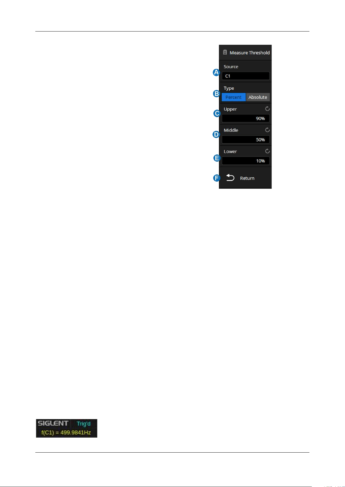
SDS6000L User Manual
int. s i g l e n t . c o m 1 7 9
A. Set measurement threshold source
B. Set the type of threshold
C. Set the upper value
D. Set the middle value
E. Set the lower value
F. Return to the previous menu
Threshold Type
Percent:
Set according to the percentage of the waveform. The setting range of lower value and upper
value is 1% ~ 99%, and the low value shall not be greater than the middle value and high value
Absolute:
Set according to the vertical range. The absolute threshold value depends on the vertical
scale, offset and probe attenuation. These values should be set before setting absolute thresholds.
Lower and upper values are limited to the range of the screen. If any absolute threshold is greater or
less than the minimum or maximum waveform value, the measurement may be invalid.
16.13 Hardware Frequency Counter
The hardware frequency counter is a stand-alone, hardware-based frequency measurement function.
Differing from the “Frequency” parameter (see section “Horizontal Measurement”) which is measured
by software, the hardware frequency counter directly uses the trigger signal as the input of a hardware
counter, which yields 7-digit frequency measurement accuracy. The accuracy of the “Frequency”
parameter measured by software is relative to the sample rate. The lower the sample rate, the worse
the accuracy. In situations where the sample rate is less than 2 times the input frequency, the results
will be incorrect. The hardware frequency counter does not have this limitation. Its result is always
shown at the top-right of the display as shown below:
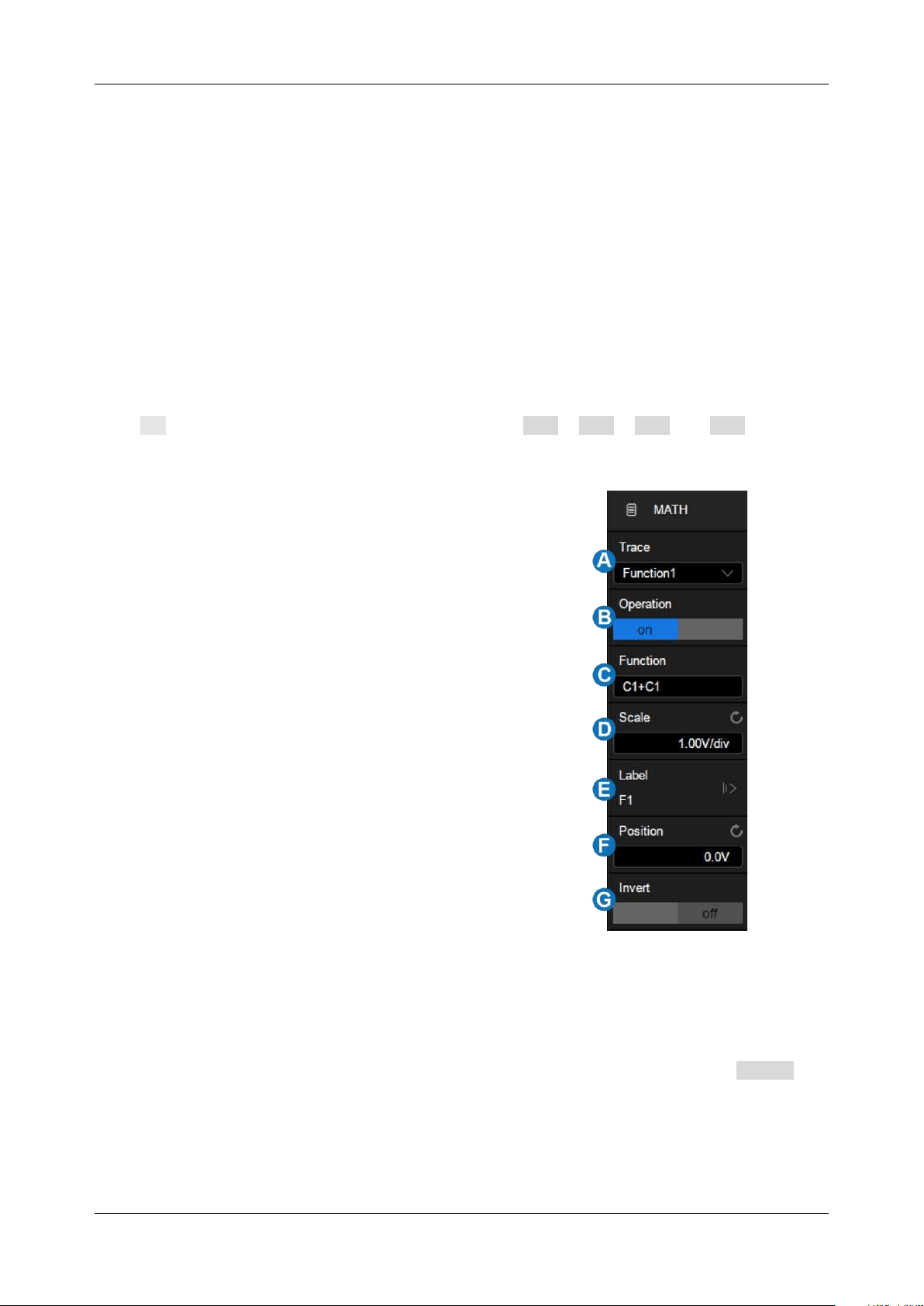
SDS6000L User Manual
1 8 0 i n t . s i g l e n t . c o m
17 Math
17.1 Overview
The SDS6000L supports 4 math traces and multiple operators. Arithmetic operators: Addition (+),
subtraction (-), multiplication (x), division (/), average, ERES, identity, negation, maxhold, minhold.
Algebra operators: differential (d/dt), integral (∫dt), square root (√), absolute (|y|), sign, exp, ln,
interpolate; and FFT, Filter, as well as a formula editor. The math traces are labeled with icons “F1 ~
F4” and can be measured by the cursors or as the source of auto measurement.
Click + in the channel descriptor box region and select F1 , F2 , F3 , or F4 , and then
the math dialog box pops up.
A. Select the math trace, F1-F4
B. Turn on or off the math operation
C. Select the function. Click the area to recall the
function setting page, and select the source and
operator
D. Set the vertical scale of the math operation
E. Set the label text of the math trace
F. Set the vertical position of the math operation,
referring to "Vertical Setup"
G. Enable/Disable Invert, similar to the process used
in "Vertical Setup".
Units for Math Waveform
Different operations have different dimensions. Therefore, the specific units displayed in Scale
depend on the operation:

SDS6000L User Manual
int. s i g l e n t . c o m 1 8 1
Math Operation
Unit
Addition (+) or
Subtraction (-)
V, A, or U*
*(used when the units of two sources are not consistent)
Multiplication (x)
V
∧
2, A
∧
2, or W
Division (/)
None, Ω (Resistance unit Ohms), S (conductance unit Siemens)
FFT
dBVrms, Vrms, dBArms, Arms, dBm
d/dt
V/s (Volt/second) or A/s (A/second)
∫dt
VS (Volt*second) or AS (A*second)
√
V
∧
0.5 or A
∧
0.5
|y|
V, A
Sign
V, A
Exp or Exp10
V, A
Ln or lg
V, A
intrp
V, A
17.2 Arithmetic
The SDS6000L supports Addition, Subtraction, Multiplication, Division, Average, ERES, Identity,
Negation, Max-hold, and Min-hold.
17.2.1 Addition / Subtraction / Multiplication / Division
The SDS6000L can perform arithmetic operations including addition, subtraction, multiplication, or
division on any two analog input channels, and the values of Source A and Source B are computed
point-by-point.
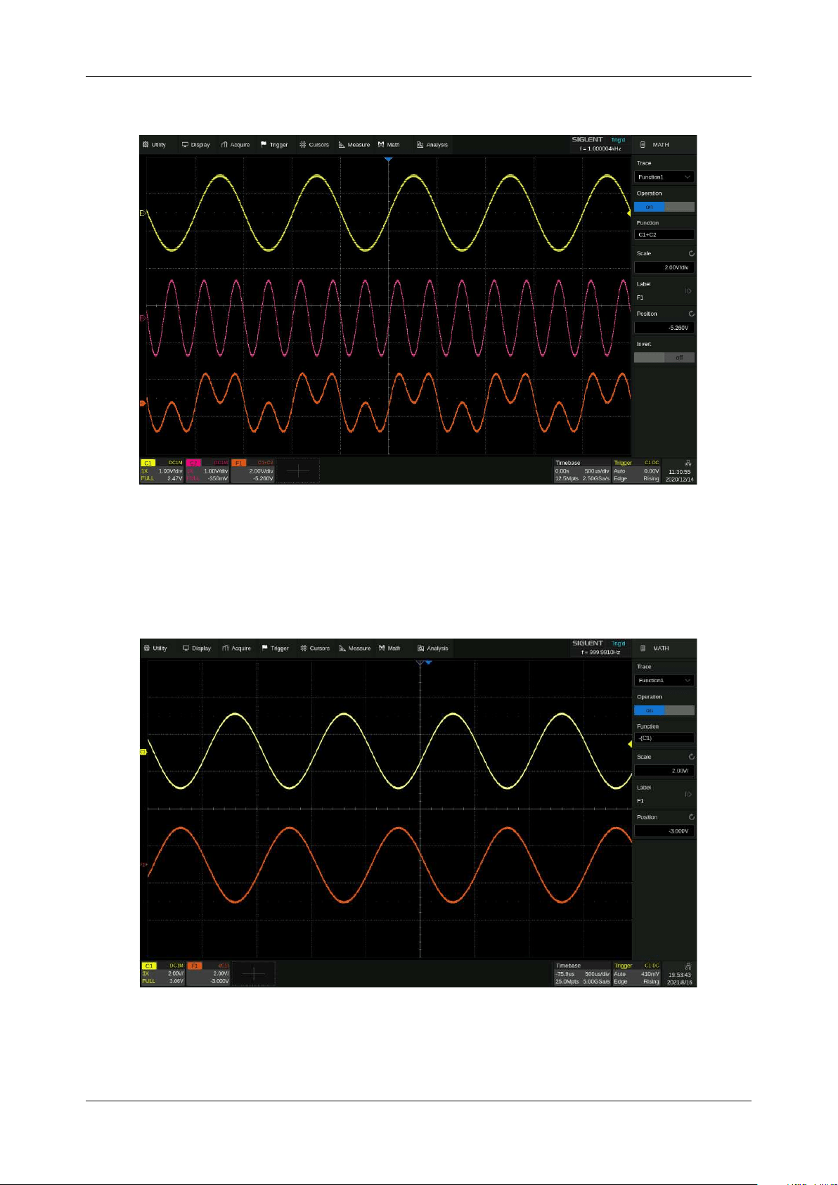
SDS6000L User Manual
1 8 2 i n t . s i g l e n t . c o m
The following figure shows an example of F1 = C1 + C2:
17.2.2 Identity / Negation
The values of Source A are computed point-by-point when an identity or negation operation is chosen
in any analog channel. The following figure shows an example of F1 = -C1:
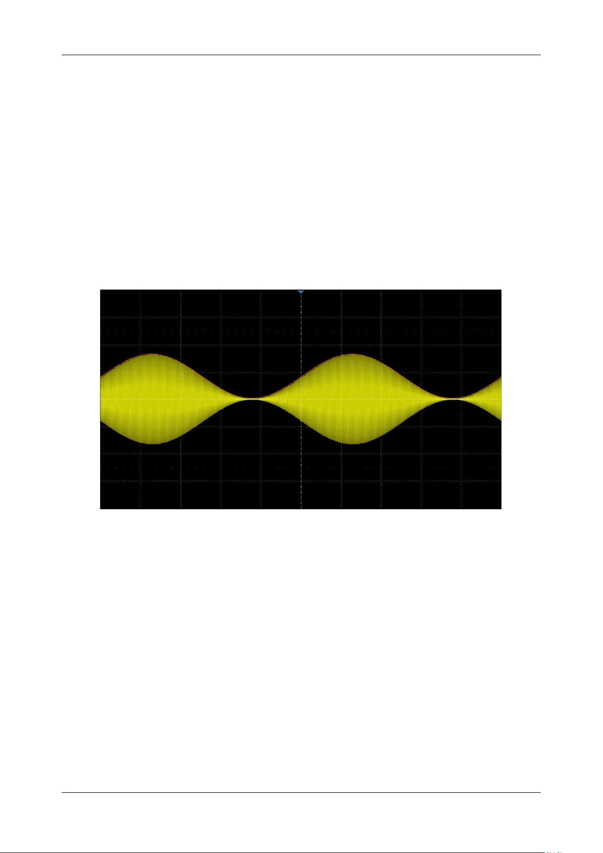
SDS6000L User Manual
int. s i g l e n t . c o m 1 8 3
17.2.3 Average / ERES
Average / ERES can be set in acquisition mode and arithmetic function as well, but with different
computing methods. Average and ERES in acquisition mode are computed by hardware with a higher
speed than if they were computed by software in the arithmetic mode. Average and ERES in acquisition
mode can only be based on data from analog channels, while the Average / ERES arithmetic function
can use analog channels, zoom traces, math, and memory traces as the source.
17.2.4 Max-hold / Min-hold
The value of Max-hold and Min-hold are based on statistical calculations from multiple frames. The
following figure shows the Max-hold result.
17.3 Algebra
The SDS6000L can perform algebraic operations including differential (d/dt), integral (∫dt), square root
(√), absolute(|x|), sign, exp (
), exp10 (
), ln, lg and interpolate (Intrp).
17.3.1 Differential
The differential (d/dt) operator is used to calculate the derivative of the selected source. It is always
used to measure the instantaneous slope of the waveform, such as the slew rate of an operational
amplifier.
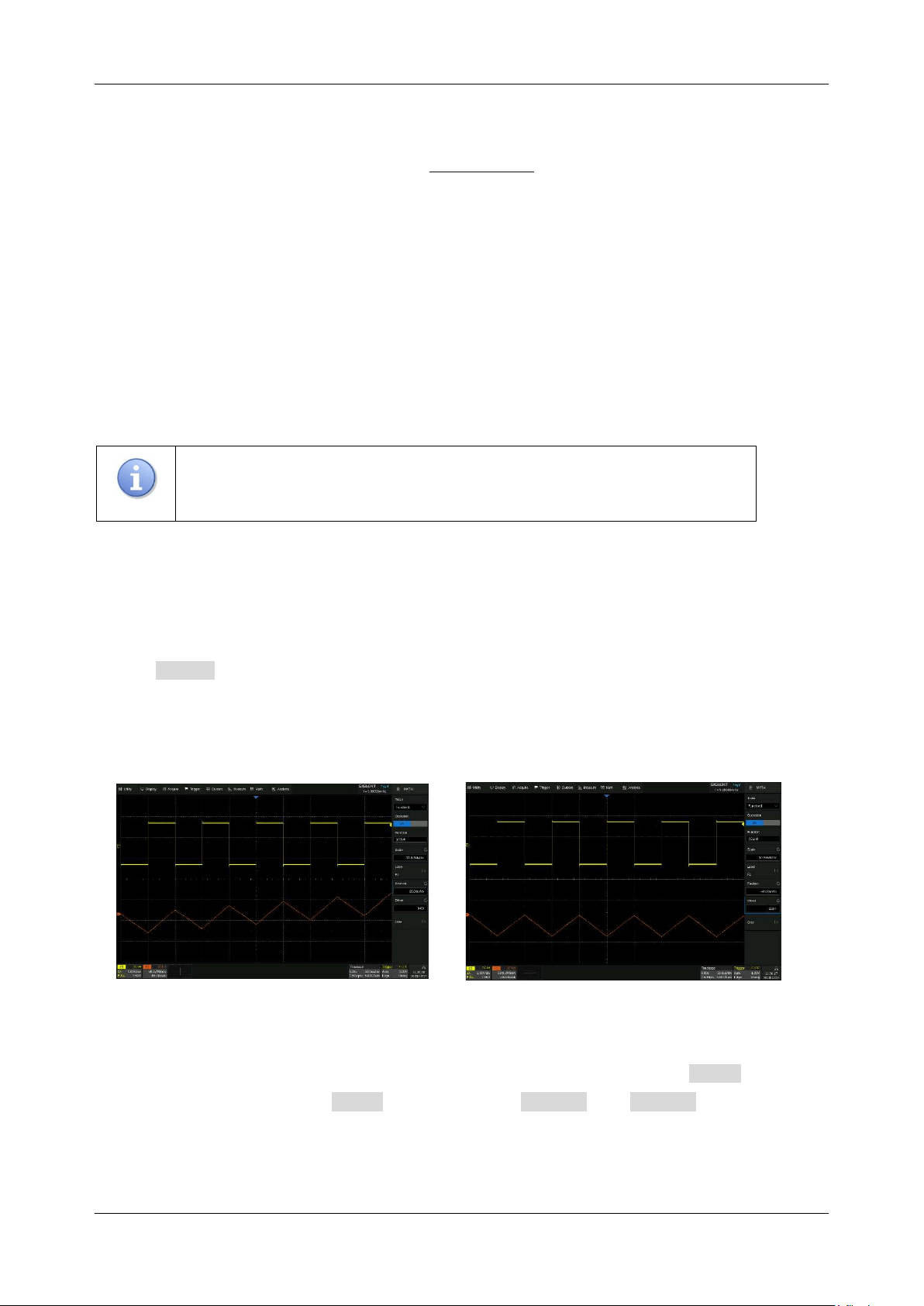
SDS6000L User Manual
1 8 4 i n t . s i g l e n t . c o m
The differential equation is:
dx
y(i) - dx)+(iy
di =
Where:
d = Differential result
y = Values of source data
i = Data point index
dx = Differential interval
The range of “dx” in the d/dt menu is 4~ number of samples pts.
Note:
Differentiation is sensitive to noise. It is helpful to set the acquisition mode
to “Average” or “ERES” to help minimize the visible effects of additional noise.
17.3.2 Integral
Integral operation integrates the waveforms on the screen or within the specified gate.
Setting Offset in the integral menu provides an approach to correct the DC offset of the source.
Small DC offsets in the input signal (or even small offset errors of the oscilloscope itself) may cause
the integral output waveform to "ramp" up or down, as shown below:
Integral without Offset
Integral with Offset
In addition, the integral operation can be performed within a specified gate. Click Gate area in the
math dialog box, and enable the Gate function, then set Gate A and Gate B to define the gate.
The setting of the gate cursors is similar to that of normal cursors. See "Select and Move Cursors" for
details.
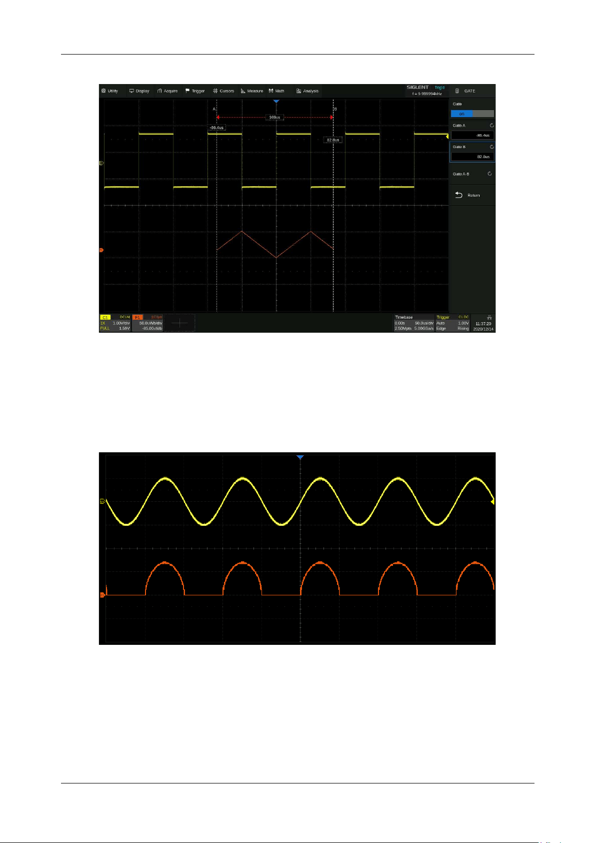
SDS6000L User Manual
int. s i g l e n t . c o m 1 8 5
17.3.3 Square Root
Square root
(
√
)
calculates the square root of the selected source. If the waveform value is negative
(the waveform is below the ground level), the result is displayed as zero.
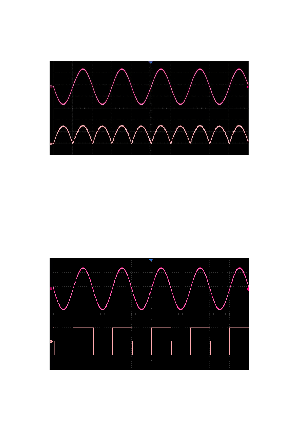
SDS6000L User Manual
1 8 6 i n t . s i g l e n t . c o m
17.3.4 Absolute
Absolute (|x|) calculates the absolute value of the selected trace.
17.3.5 Sign
In mathematics, the sign function or signum function (from signum, Latin for "sign") is an odd
mathematical function that extracts the sign of a real number.
The sign function of a real number x is defined as follows:
Sign(x) = -1
if x < 0,
= 0
if x = 0,
= 1
if x > 0.
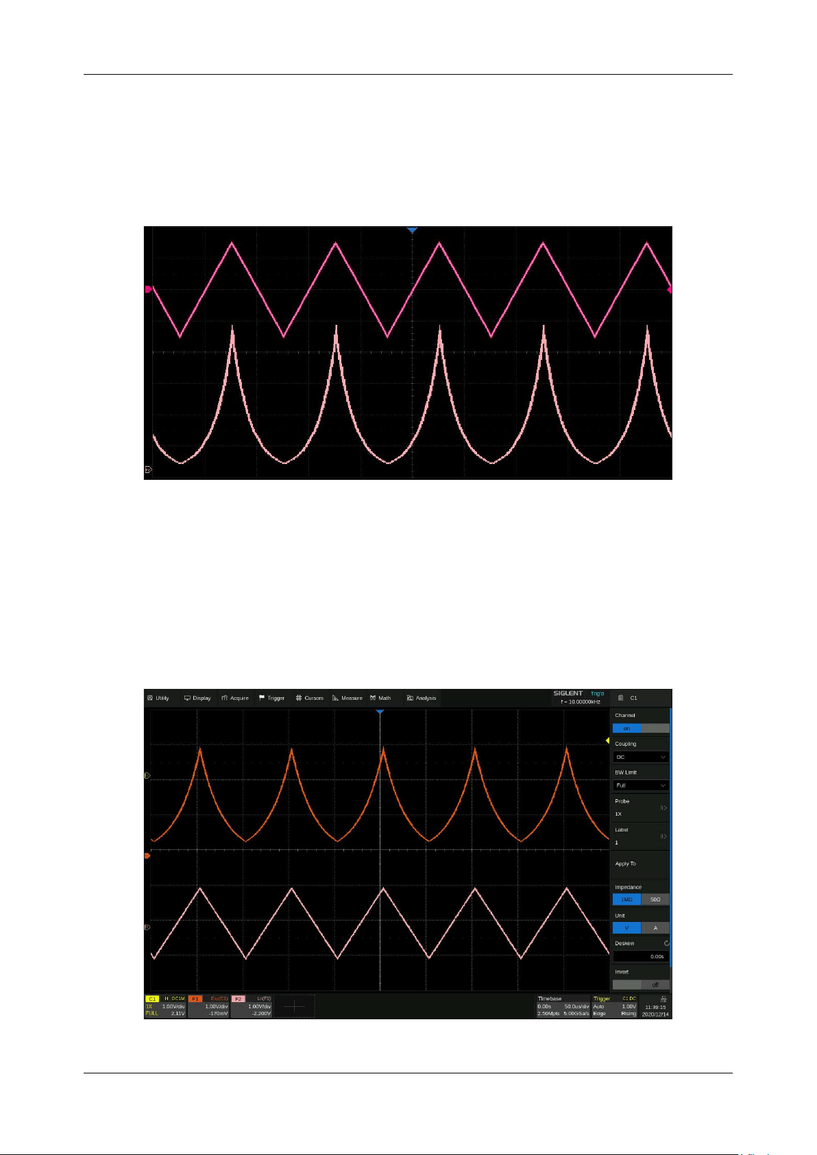
SDS6000L User Manual
int. s i g l e n t . c o m 1 8 7
17.3.6 exp/exp10
The exponential operation includes the exponential operation
based on constant e and the
exponential operation
based on 10.
For example: y(x) =
.
17.3.7 ln/lg
Logarithmic operation includes logarithm base e (ln) and logarithm base 10 (lg). In logarithmic
operation, if the waveform value is negative (the waveform is below the ground level), the result is
displayed as zero.
For example, F1 =
, where x is the trigonometric wave function. F2 = ln (F1).
SDS6000L User Manual
1 8 8 i n t . s i g l e n t . c o m
17.3.8 Interpolate
Between the adjacent sampling points, the waveform is interpolated according to the selected
interpolation method and interpolation coefficient. Click Acquire > Interpolation to set the
interpolation method, and the interpolation coefficient can be set to 2, 5, 10, or 20.
coefficient = 2
coefficient = 20
17.4 Filter
The filter operation in the SDS6000L provides FIR (Finite Impulse Response) filtering with the following
types: Low pass, High pass, Bandpass, and Band Reject. The filters have up to 200 taps which can
reach roll-off as fast as 0.01*fs. Users just need to set the filter type and corner frequency(s), then the
instrument will automatically calculate the coefficients needed for the filtering.
A. Choose to let the scope set the sample rate
automatically according to the filter setting or
not. See below for details
B. Filter type: Low pass, High pass, Bandpass,
and Band Reject
C. Corner frequency. For Bandpass and Band
Reject there are two corner frequencies,
separately named Lower Frequency and Upper
Frequency. The attenuation at the corner
frequency is around 3 dB
SDS6000L User Manual
int. s i g l e n t . c o m 1 8 9
Adapt Sample Rate
Unlike an ideal “brick wall” filter, the actual FIR filters have their roll-off from the passband to the
stopband because of the limited number of taps. The 200-tap FIRs applied in the SDS6000L provide
roll-off as fast as 0.01*fs (where fs is the sample rate), this means some limitations in the setting of
corner frequency at a specified sample rate. The figures below show the limitations in detail:
≥0.01fs ≥0.01fs
fs/2fc
≥0.01fs ≥0.01fs
fs/2fc
Low pass
High pass
≥0.01fs
≥0.01fs
fs/2
fl
≥0.02fs
fh
≥0.01fs ≥0.01fs
fs/2
fl
≥0.02fs
fh
Bandpass
Band reject
Take a Low pass filter as an example. It requires that the corner frequency (fc) is not less than 0.01*fs
(i.e. fc ≥ 0.01*fs), and the 0.01*fs wide roll-off does not exceed the 1st Nyquist zone (i.e. (fs/2) - fc ≥
0.01fs). If fs = 5 GSa/s, then the legal range of the corner frequency (fc) is 50 MHz~2450 MHz
If the expected fc is out of the legal range at some sample rate, then the sample rate needs to be
changed. For instance, when fs = 5 GSa/s, the setting fc = 10 MHz is illegal, so we must lower fs to 1
GSa/s to satisfy the limitation (fc ≥ 0.01*fs).
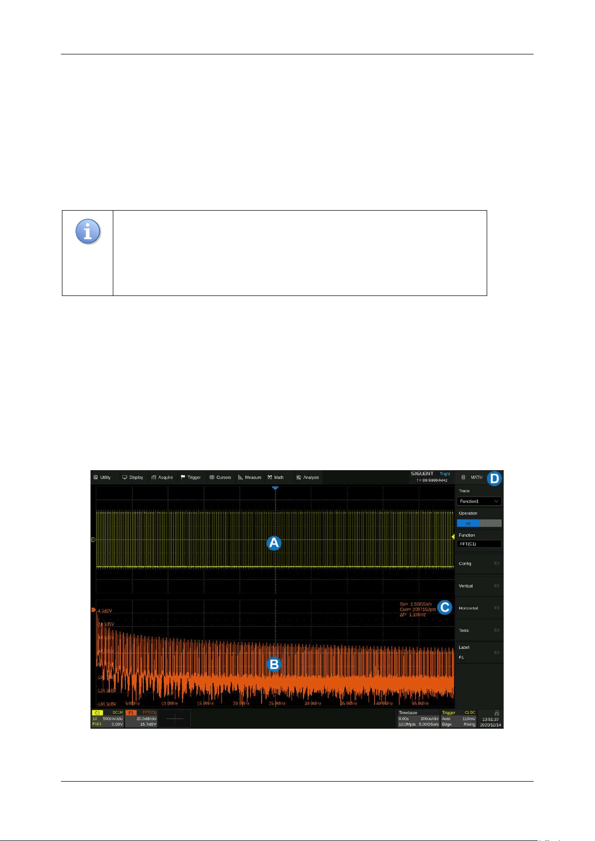
SDS6000L User Manual
1 9 0 i n t . s i g l e n t . c o m
Professional users who have prior knowledge of FIR filters and are familiar with the operation of this
instrument are encouraged to change the sample rate for the corner frequency of interest. Otherwise,
we recommend using the “Adapt Sample Rate” option. In this mode, the scope forces the Memory
Management Mode to be “Fixed Sample Rate” and automatically adjusts the sample rate to adapt to
the corner frequency setting. For details of the Memory Management Mode refer to the section
“Memory Management”.
Note:
Be aware that when the corner frequency is set very low the sample rate
may not satisfy the Nyquist Theorem (i.e. fs is no longer greater than or equal
to twice the highest frequency of the input). Keep the sample rate reasonable
at all times.
17.5 Frequency Analysis
The result of FFT (Fast Fourier Transform) calculations is the frequency spectrum of the source signal.
The horizontal axis of the FFT display is labeled using frequency (Hz) units instead of time (seconds).
In addition, the vertical axis provides the option of logarithmic scaling (dBVrms/dBArms or dBm).
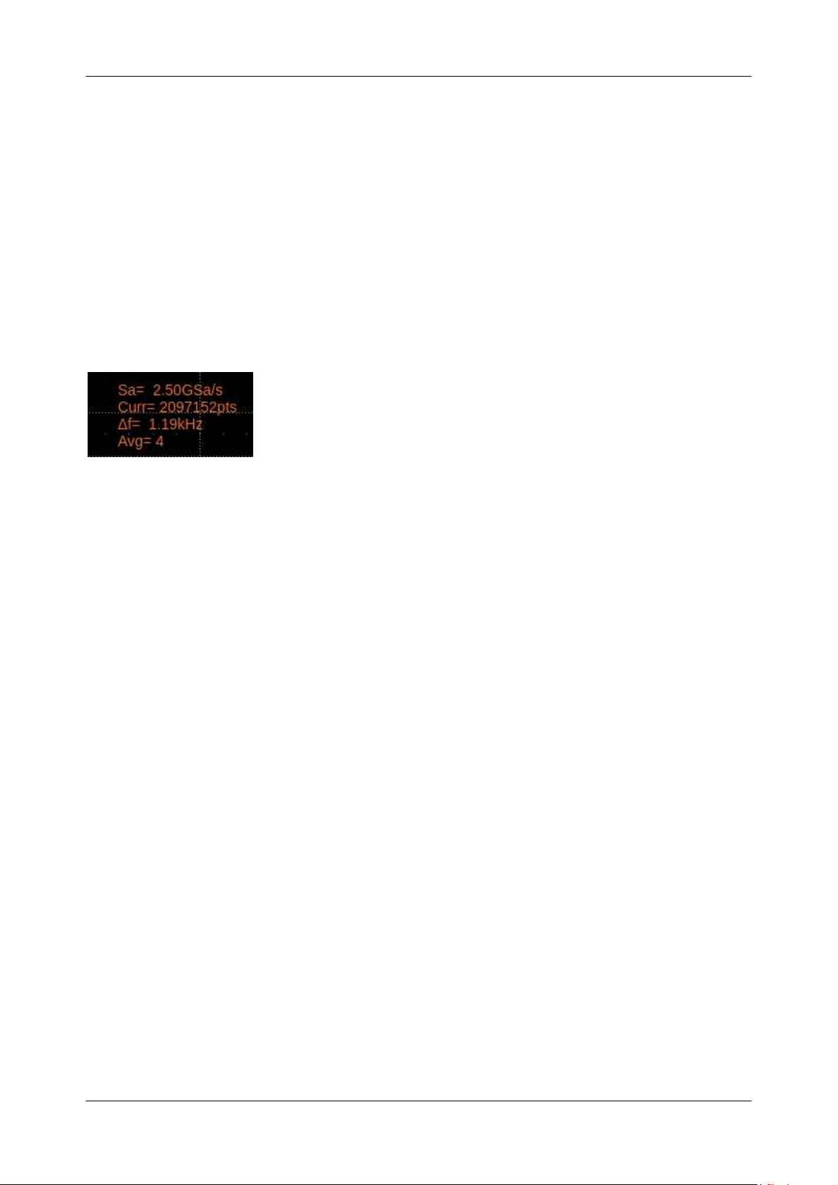
SDS6000L User Manual
int. s i g l e n t . c o m 1 9 1
A. Time-domain waveform display area
B. Spectrum (FFT) waveform display area
C. FFT parameter display area
D. Dialog box
Parameter Display Area
The FFT parameters are displayed in the upper right of the spectrum waveform display area:
FFT sample rate (Sa):
FFT operation results present the first Nyquist zone (DC ~ Sa/2) of the
frequency spectrum. Be aware that the FFT sample rate may be inconsistent with the sample rate
in the time domain. Assuming the max points value is set to 2 Mpts:
✓ When the number of points in the time domain, N, is less than 2 Mpts, the FFT takes the
number which is an integer power of 2 closest to N. In this case, FFT sample rate = sample
rate in the time domain.
✓ When N is greater than 2 Mpts, FFT first decimates N by D and then takes the first 2 Mpts
for the calculation. In this case, FFT sample rate = sample rate in time domain/D.
For example, in the case of sample rate in the time domain is 5 GSa/s and the number of
samples is 5 Mpts, the FFT first decimates the samples by 2, to 2.5 Mpts, and then takes the
first 2 Mpts to calculate the spectrum. In this example, FFT sample rate = 5 GSa/s ÷ 2 = 2.5
GSa/s.
FFT points (Curr):
The current FFT points, which is an integer power of 2. The SDS6000L
supports up to 8 M points (8388608, to be exact).
Frequency interval (
△
f):
The frequency interval between two adjacent points in the FFT
sequence, which is proportional to the frequency resolution.
Average count of FFT (Avg):
Displayed only when the FFT mode is set to "Average", indicating
the completed average count.
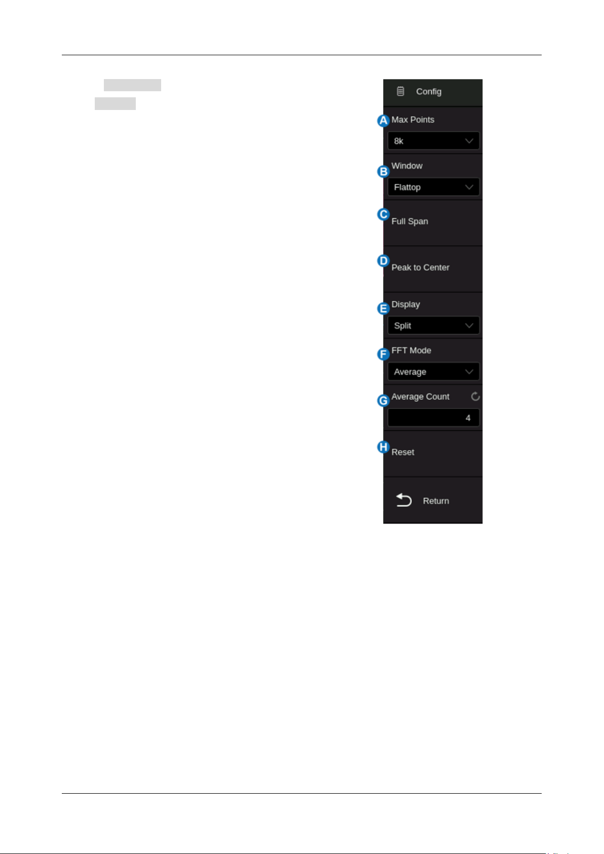
SDS6000L User Manual
1 9 2 i n t . s i g l e n t . c o m
Select Operation as FFT in the math dialog box and
click Config to recall the configuration dialog box:
A. Set the maximum points (2
n
, n = 10 ~ 23)
B. Set the window type (Rectangle, Blackman,
Hanning, Hamming, and Flattop)
C. Automatically set the horizontal axis to fall
span
(
0~f
s
/2
)
D. Automatically set the center frequency to the
maximum frequency component in the
previous frame
E. Select the display mode (Split, Full Screen,
and Exclusive)
F. Select the FFT mode (Normal, Average, and
Max-Hold)
G. Set the average count in average mode
H. Reset average
Windows
Spectral leakage in FFTs can be considerably decreased when a window is used. SDS6000L provides
five windows that have different characteristics and apply to different scenarios.
For example, for a two-tone signal with a very close frequency interval, it is suitable to use a Rectangle
window with the best frequency resolution. For the case where the accuracy of amplitude measurement
is critical, it is recommended to select the Flattop window with the best amplitude resolution.
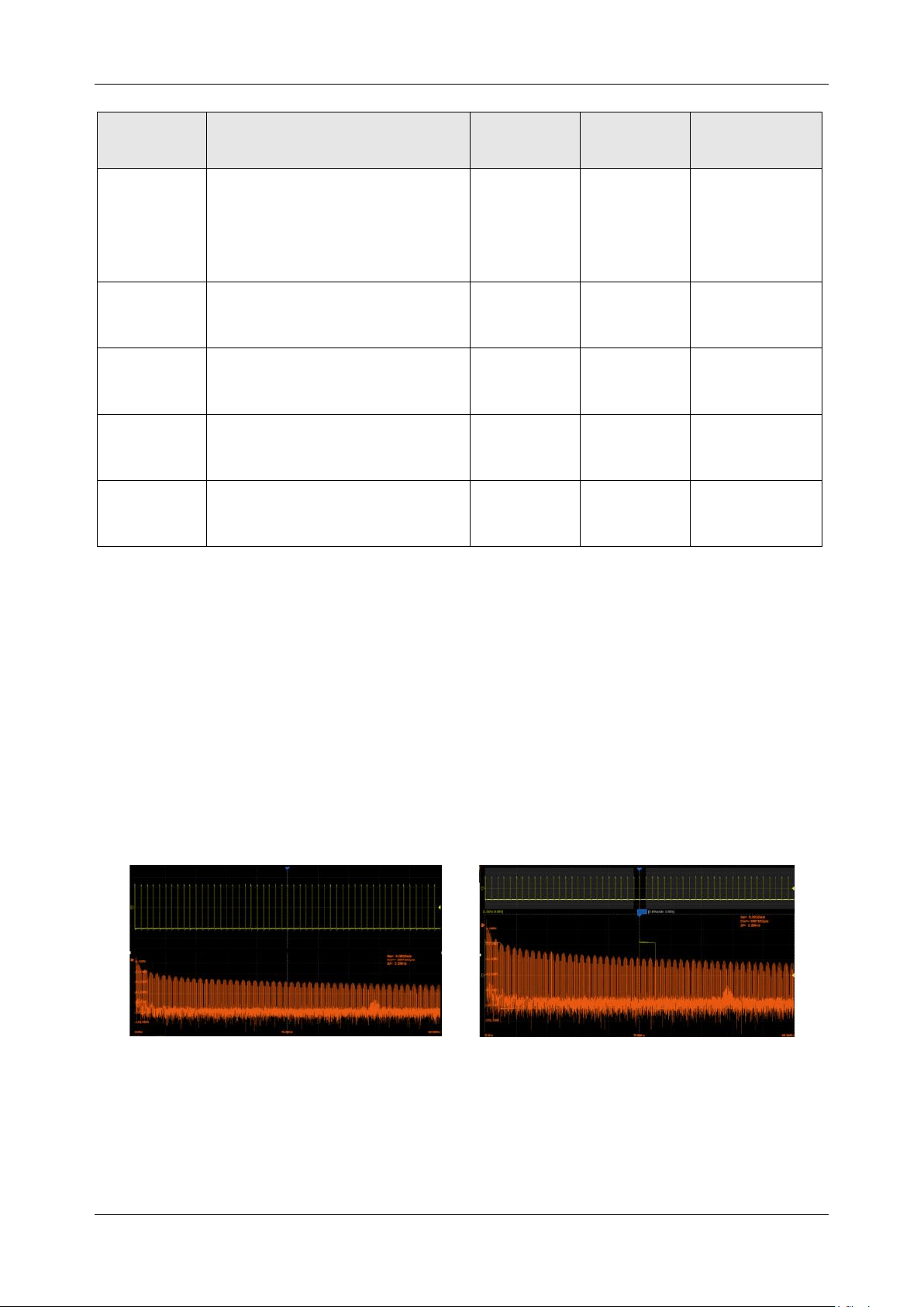
SDS6000L User Manual
int. s i g l e n t . c o m 1 9 3
Window
Characteristics
Main lobe
width
Side lobe
suppression
Maximum
amplitude error
Rectangle
The best frequency resolution
The worst amplitude resolution
It is equivalent to the case of
no window
4π/N
-13 dB
3.9 dB
Hanning
Better frequency resolution
Poor amplitude resolution
8π/N
-32 dB
1.4 dB
Hamming
Better frequency resolution
Poor amplitude resolution
8π/N
-43 dB
1.8 dB
Blackman
Poor frequency resolution
Better amplitude resolution
12π/N
-58 dB
1.1 dB
Flattop
The worst frequency resolution
The best amplitude resolution
23π/N
-93 dB
< 0.1dB
Display Mode
Split:
Time-domain waveform and frequency-domain waveforms are displayed separately. The
time-domain waveform is on the upper half screen, while the frequency-domain waveform is
located within the lower half of the display. In Split mode, if Zoom is enabled, the zoomed waveform
and the frequency domain waveform are displayed on the lower half screen together.
Full Screen:
Time-domain waveform and frequency-domain waveform are displayed together.
Exclusive:
Only the frequency-domain waveform is displayed.
Split Mode, Zoom off
Split Mode, Zoom on
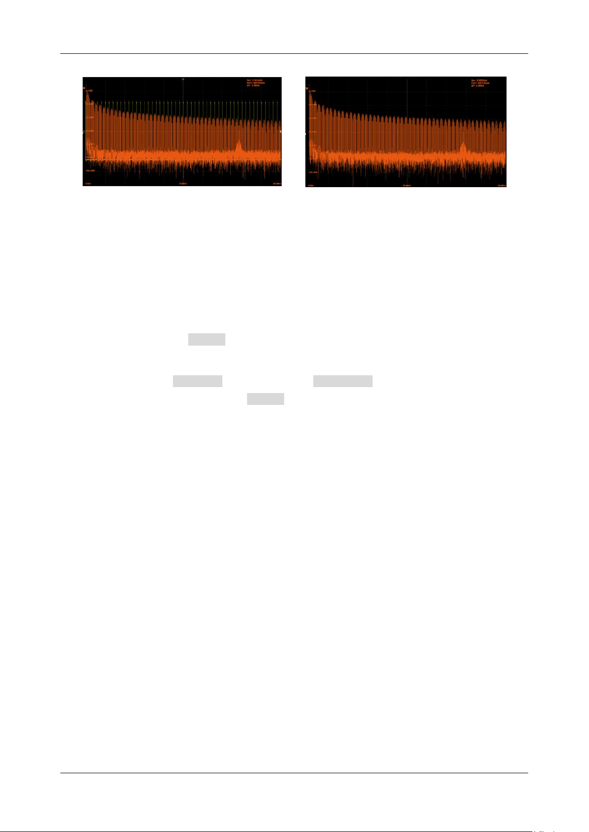
SDS6000L User Manual
1 9 4 i n t . s i g l e n t . c o m
Full-Screen Mode
Exclusive Mode
FFT Mode
Normal:
Displays the FFT result of each frame directly.
Max-Hold:
Holds the maximum value in the historic frame on the display until cleared. This mode
is suitable for detecting discontinuous waves, such as sporadic pulse signals, or frequency
hopping signals. Click Reset in the dialog box to clear the max-hold waveform.
Average:
Reduces the effect of the superimposed random noise on the signal. After the FFT mode
is set as Average, Average will appear under FFT Mode . The average count can be set
here, ranging from 4 to 1024. Click Reset in the dialog box to restart the average counter.
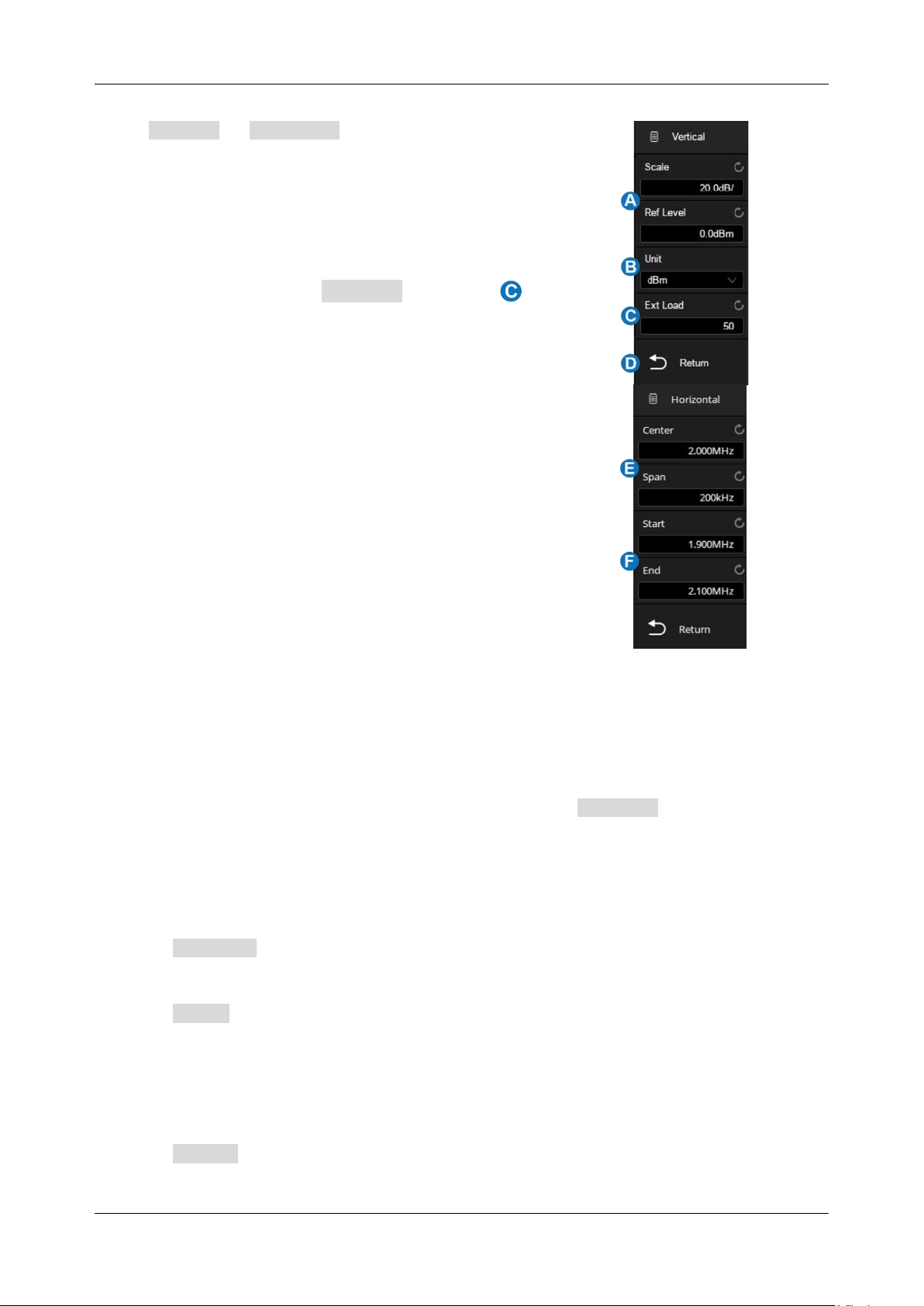
SDS6000L User Manual
int. s i g l e n t . c o m 1 9 5
Click Vertical or Horizontal in the math dialog box to
recall the FFT vertical or horizontal settings dialog box:
A. Set the vertical scale and reference level
B. Set the unit (dBVrms, Vrms, and dBm). When the unit
is dBm, the oscilloscope will automatically calculate the
dBm value based on the Ext Load value set in
area
C. Set the external load, which is used to calculate the
correct dBm result
D. Return to the previous menu
E. Set the center-span frequencies
F. Set the start-end frequencies
Unit
The unit of the vertical axis can be set to dBm, dBVrms, or Vrms. dBVrms and Vrms respectively using
either logarithmic or linear scaling. dBVrms is recommended to show larger dynamic ranges. dBm is a
power unit, the correct result can be obtained only if the value of Ext Load is set to be consistent
with the load impedance of the actual measured signal.
Vertical Control
Click Ref Level to set the reference level of the FFT waveform by the mouse wheel or the virtual
keypad.
Click Scale to set the vertical scale of the FFT waveform by the mouse wheel or the virtual
keypad. The reference point for vertical scale scaling is the reference level.
Horizontal Control
Click Center to set the center frequency by the mouse wheel or the virtual keypad.
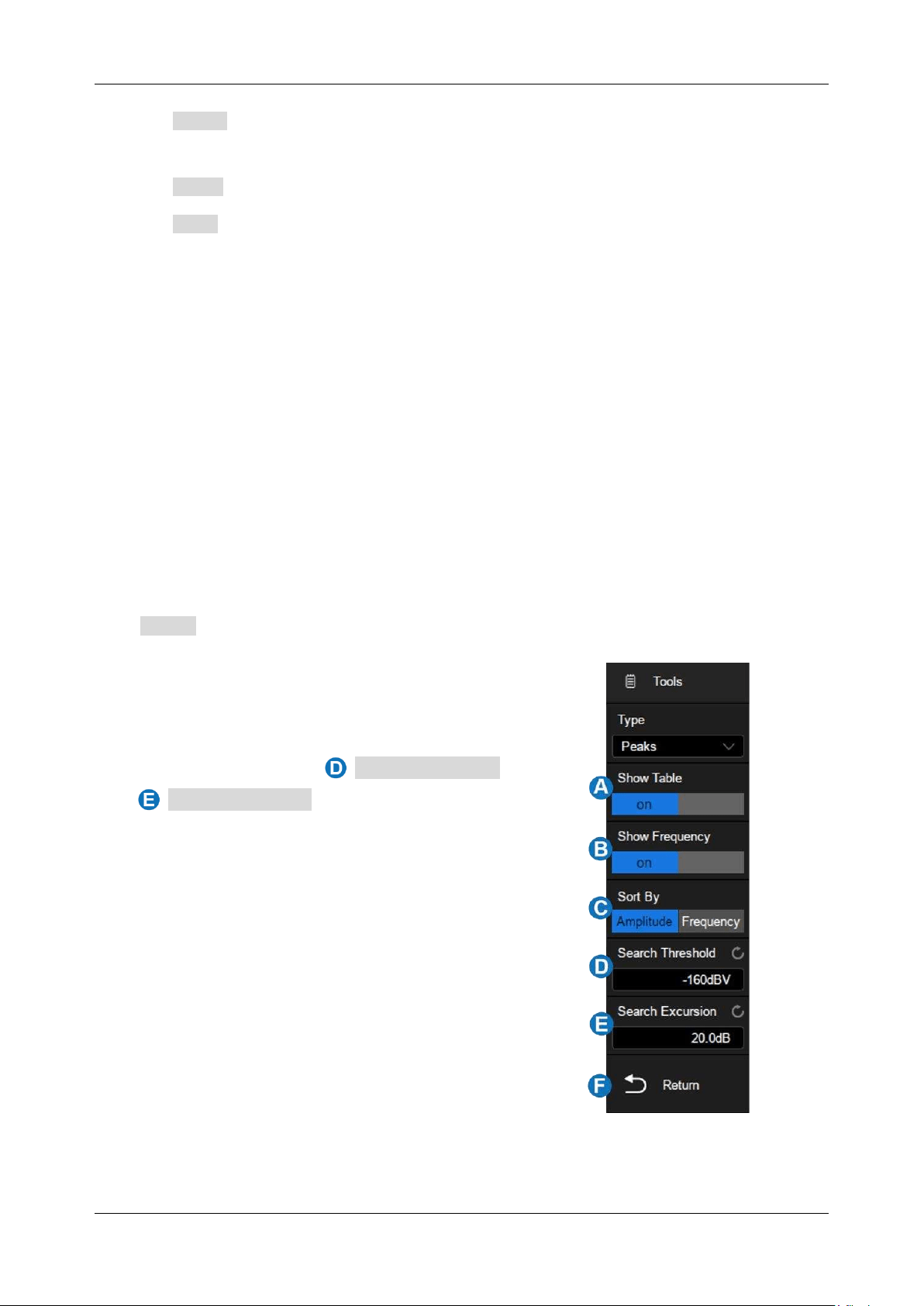
SDS6000L User Manual
1 9 6 i n t . s i g l e n t . c o m
Click Span to set the frequency span with the center frequency as the center by the mouse
wheel or the virtual keypad.
Click Start to set the start frequency by the mouse wheel or the virtual keypad.
Click End to set the end frequency by the mouse wheel or the virtual keypad.
The relationship between Center, Span, Start, and End is:
Center = (Start + End)/2
Span = End – Start
FFT Tools
The SDS6000L provides two tools for the FFT waveform: Peaks and Markers. The peaks tool can
automatically search the qualified peak points and mark them on the FFT waveform. Up to 10 peaks
are supported. Based on the peak tool, the markers tool can automatically search the qualified
harmonics, and users can control the position of each marker. Up to 8 markers are supported.
Click Tools in the math dialog box to recall the FFT tools dialog box:
When the FFT tool peaks is selected, the dialog box is as
follows:
A. Turn on or off the table. Turn on the table, the peaks
searched with the limit of Search Threshold and
Search Excursion will be displayed in a table
B. Turn on or off the display of peak frequency in the table
C. Sort peaks by amplitude or frequency
D. Set the search threshold. Only peaks larger than the
limit are shown
E. Set the difference between the peak value and the
minimum amplitude on both sides. The difference
should be greater than the search excursion
F. Return to the previous menu
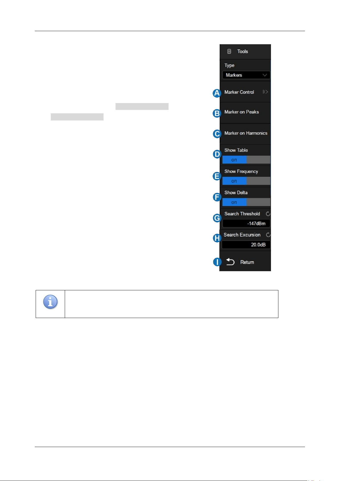
SDS6000L User Manual
int. s i g l e n t . c o m 1 9 7
When the FFT tool markers is selected, the dialog box is as
follows:
A. Control markers. Click to control the display and position
of each marker
B. Marker on peaks. It will automatically mark the peak that
meets the conditions of Search Threshold and
Search Excursion
C. Marker on harmonics. It will automatically mark each
harmonic of the FFT waveform
D. Turn on or off the table
E. Turn on or off the frequency display
F. Turn on or off the delta display
G. Set the search threshold. Only peaks larger than the
peak limit can be judged as peaks
H. Set the difference between the peak value and the
minimum amplitude on both sides. The difference should
be greater than the search excursion, which can be
determined as the peak
I. Return to the previous menu
Note:
The FFT dialog box is longer than the display. Slide the dialog box area
up and down by dragging to the view non-displayed areas.
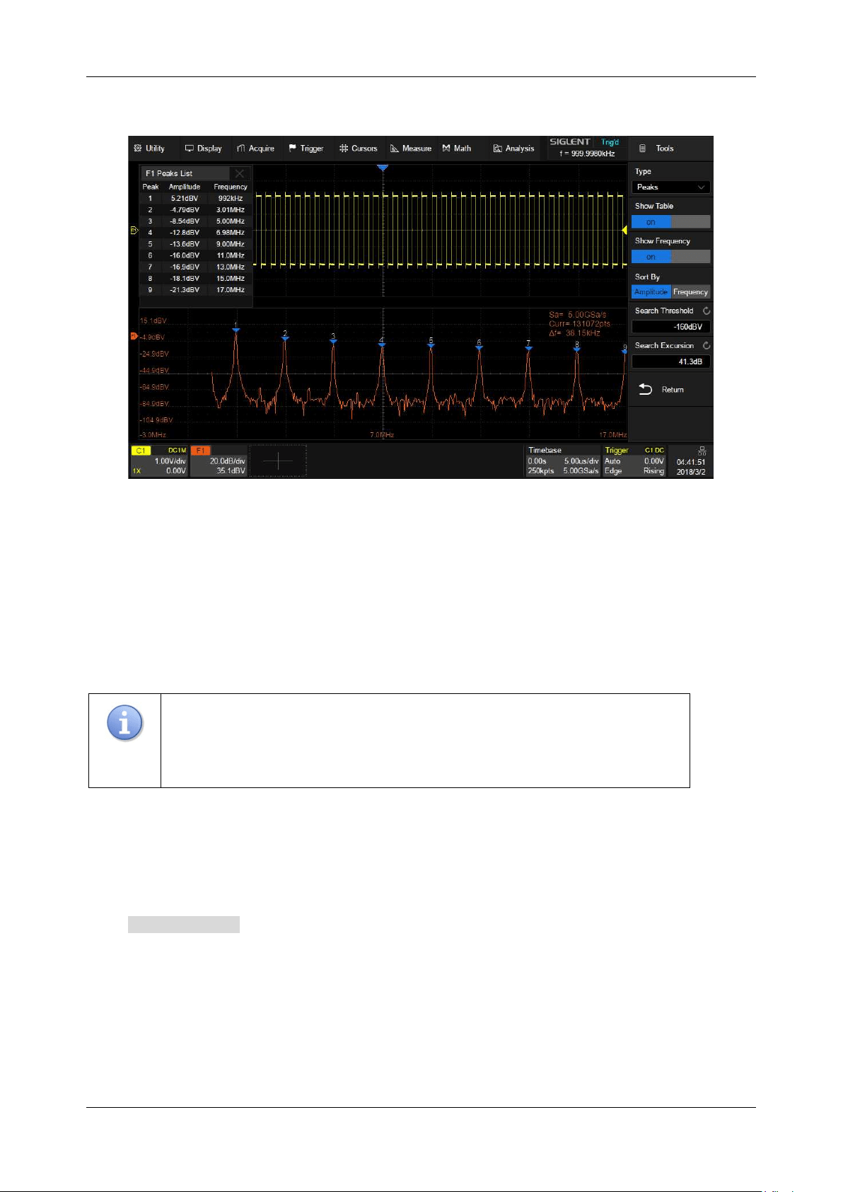
SDS6000L User Manual
1 9 8 i n t . s i g l e n t . c o m
The following screenshot shows the peaks of the FFT waveform:
Measure the FFT waveform
Turn on the cursor function, and then specify the source as "Fx". X1 and X2 cursors can be used to
measure the frequency value at the cursor position.
Only the “maximum” parameter of the FFT is supported in automatic measurement.
Note:
DC components in the signal may show a large amplitude near 0 Hz. If
your application does not require measurement of the DC component, it is
recommended to set the coupling mode of the source channel to "AC".
17.6 Formula Editor
Click Formula Editor in the operation setting page to recall the editor:
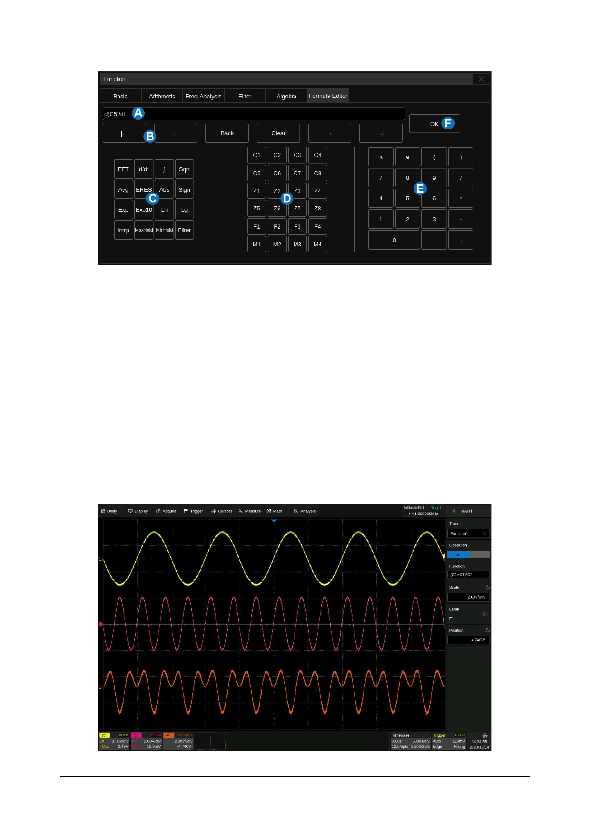
SDS6000L User Manual
int. s i g l e n t . c o m 1 9 9
A. Formula display text box
B. Text box operation area, which can clear and modify the entered formula
C. Special operators
D. Operation source. Cx represents analog trace, Zx represents zoomed trace, Fx represents math
trace and Mx represents memory trace
E. The Keyboard area contains the basic arithmetic operators addition (+), subtraction (-),
multiplication (*), division (/)
F. Confirm button. After the formula is input, press the button to apply it
The following is an example of F1 = (C1 + C1) * C2 through the formula editor
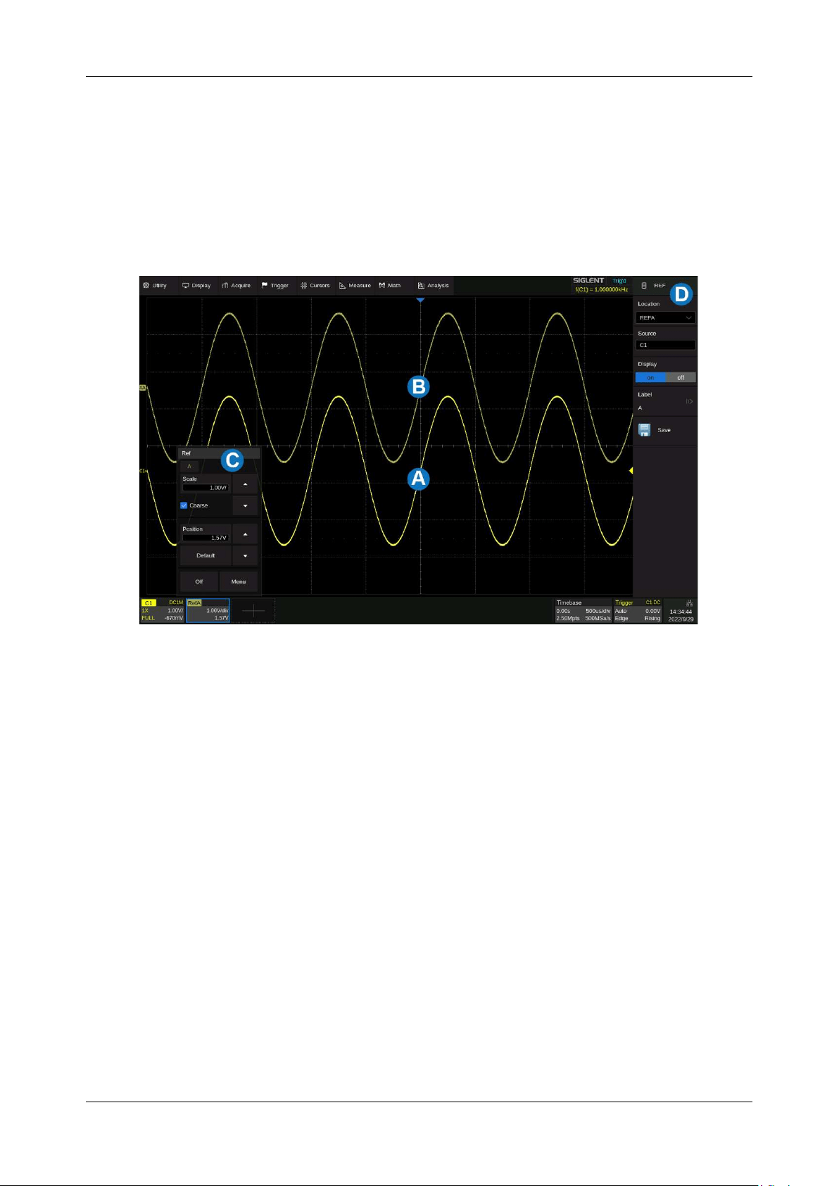
SDS6000L User Manual
2 0 0 i n t . s i g l e n t . c o m
18 Reference
Data from analog channels or math can be saved to the reference locations (REFA~H) in the built-in
nonvolatile memory. The saved reference waveform can be recalled to be compared with the current
waveform.
A. Channel waveform
B. Reference waveform
C. Reference descriptor box
D. The reference dialog box, hidden in this figure
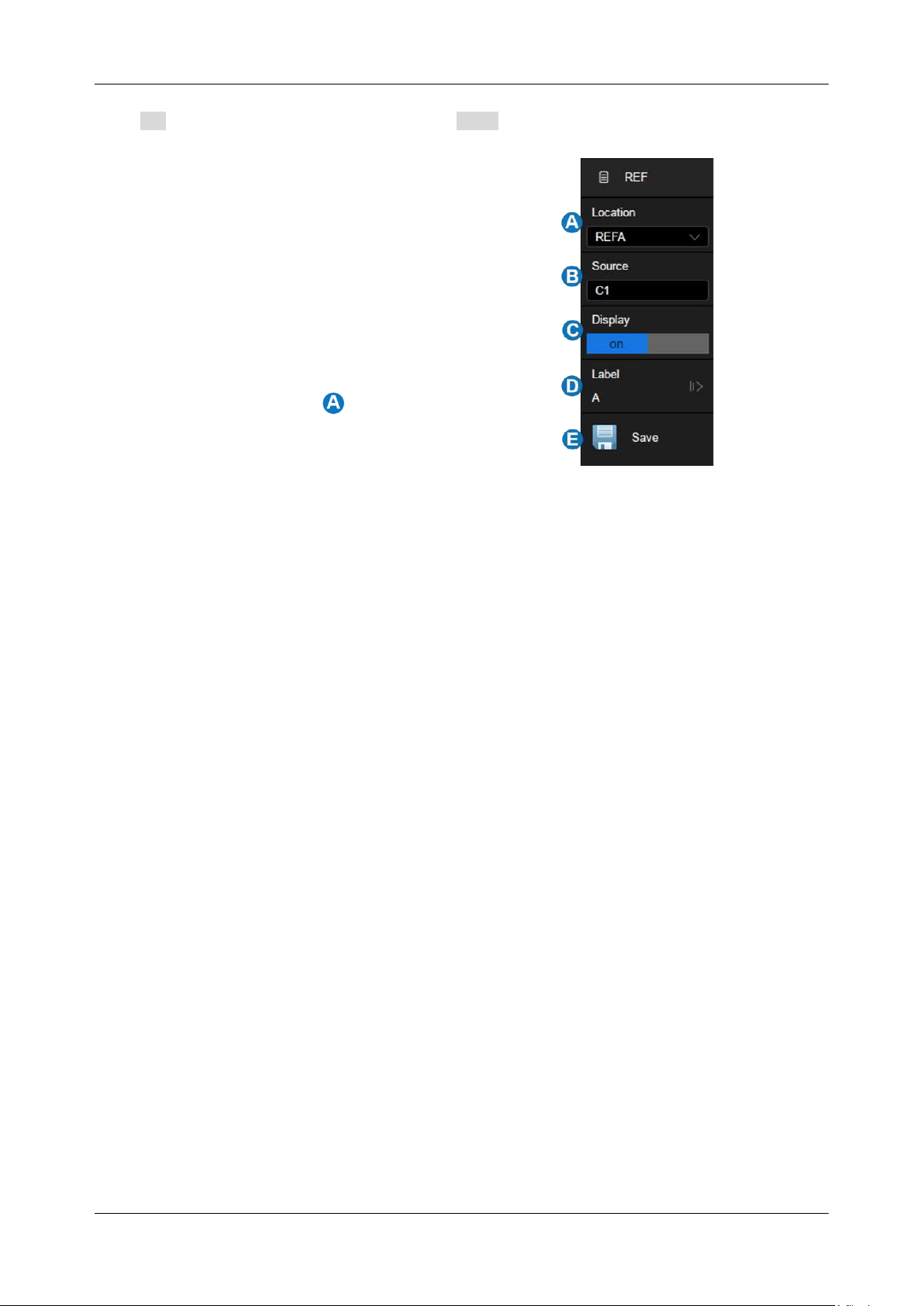
SDS6000L User Manual
int. s i g l e n t . c o m 2 0 1
Click + in the descriptor box region and select Ref to recall the ref dialog box.
A. Select the location of the reference
(REFA~REFH)
B. Select the source (C1~C8 and F1~F4)
C. Enable/disable the Display of the
reference waveform
D. Set the label text of the reference trace.
E. Save the specified waveform in/to the
specified location in
Adjust the Reference Waveform
Refer to "Vertical Setup" for adjusting the reference waveform.
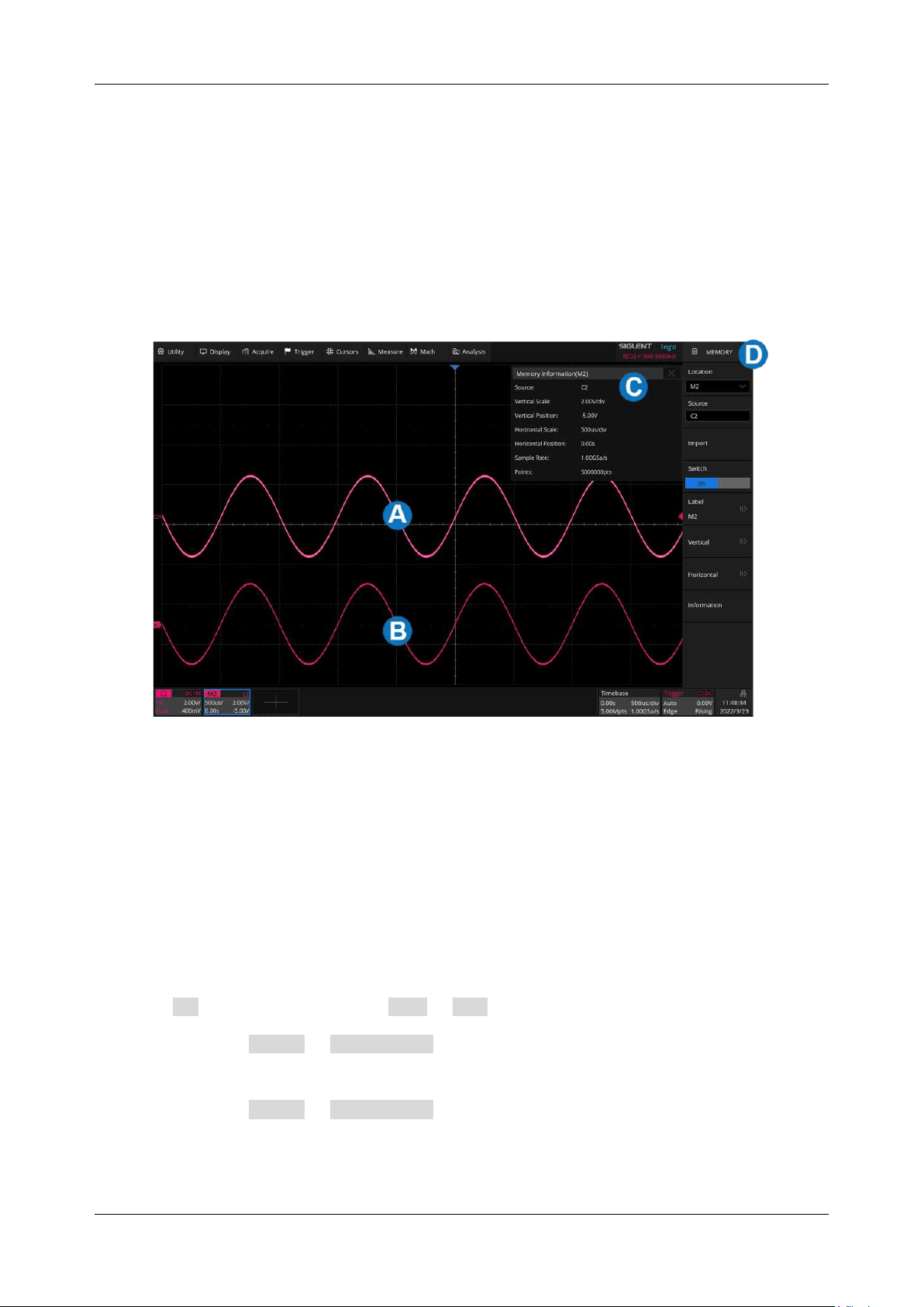
SDS6000L User Manual
2 0 2 i n t . s i g l e n t . c o m
19 Memory
Analog channels (Cx), zoom (Zx), math (Fx), memory waveforms (Mx), and waveforms in files can be
imported to available memory waveforms (M1/M2/M3/M4) and displayed on the screen for comparison
with the current waveforms. Differing from reference traces which are displayed data, the memory
traces are in the format of raw data, which can be used as the source of Math and Decoding functions
and can provide more accurate measurements than a reference waveform.
A. Channel waveform
B. Memory waveform
C. Memory information
D. The Memory dialog box
There are multiple ways to import waveforms to memory. To enter the memory dialog box:
Click + at the bottom and select M1 ~ M4 .
Click the menu Utility > Save/Recall to open the Save/Recall dialog box, select Mode as
"Save”, and Type as "To Memory".
Click the menu Utility > Save/Recall to open the Save/Recall dialog box, select Mode as
"Recall", Type as "Waveform", and then import the file to memory.
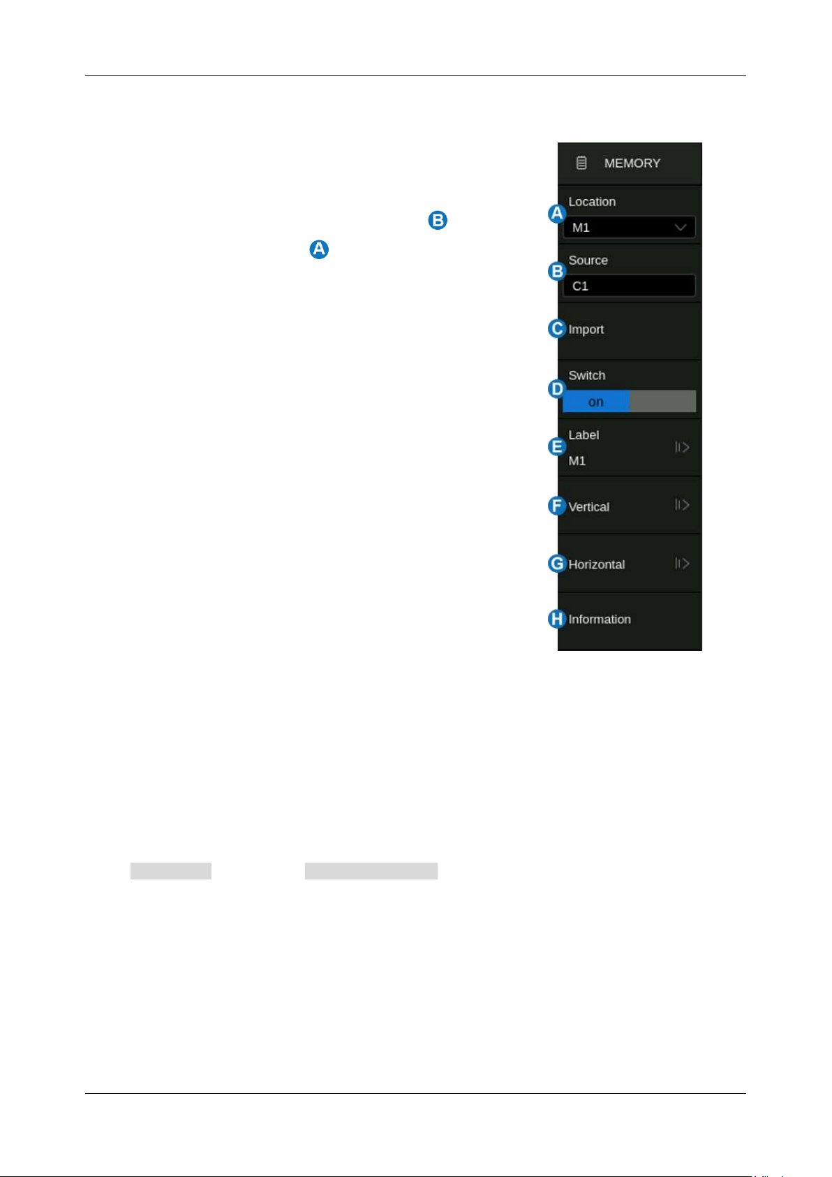
SDS6000L User Manual
int. s i g l e n t . c o m 2 0 3
Details of the dialog box are as below.
A. Select the location of the memory (M1 ~ M4)
B. Select the source (Cx / Zx / Fx / Mx / File)
C. Import the trace of the selected source in to the
memory location set in
D. Turn on or off the Memory
E. Set the label text of the memory trace
F. Set the vertical parameters of the memory trace
G. Set the horizontal parameters of the memory trace
H. Display the memory information, including source, vertical
and horizontal parameters, sampling rate, and length
Adjust the Memory Waveform
There are a couple of ways to adjust the memory waveform:
Adjust the parameters in the descriptor box of Mx at the bottom of the display
Adjust the parameters in the Memory dialog.
In the Horizontal menu, when Sync with Window option is enabled, the horizontal parameters of
the memory trace and analog traces are adjusted synchronously, otherwise, they are adjusted
separately.
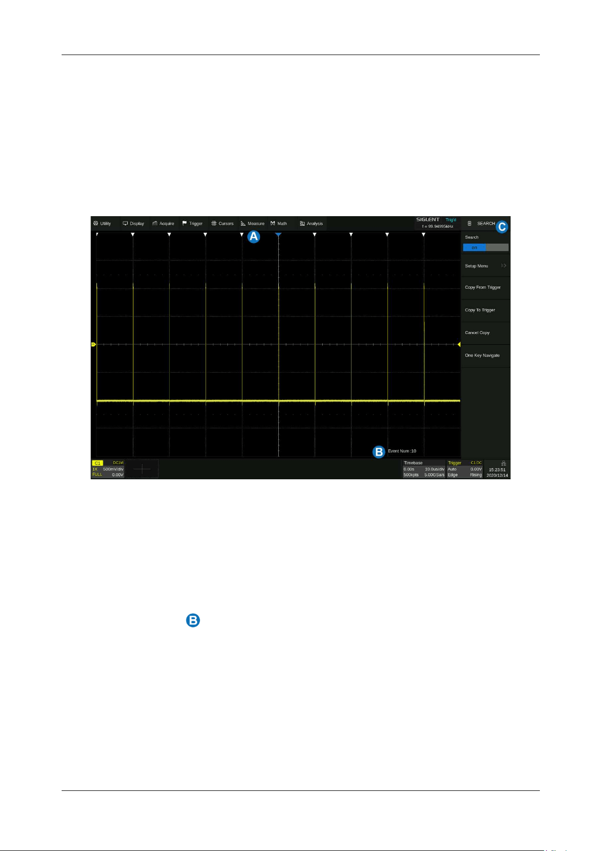
SDS6000L User Manual
2 0 4 i n t . s i g l e n t . c o m
20 Search
The SDS6000L can search for the specified events in a frame. The location of the events is displayed
with white triangle indicators. In YT mode or Roll mode with the acquisition stopped, up to 1250 events
are supported. In Roll mode with the acquisition running, the number of search events is unlimited. The
waveform can be zoomed in when the search function is enabled.
A. Search event indicator, marking the time point of an event
B. Total number of events marked on the display
C. The search dialog box, hidden in this example
In the stop state, the area shows the index of the current event/total number of events. The current
event is the one in the center of the display.
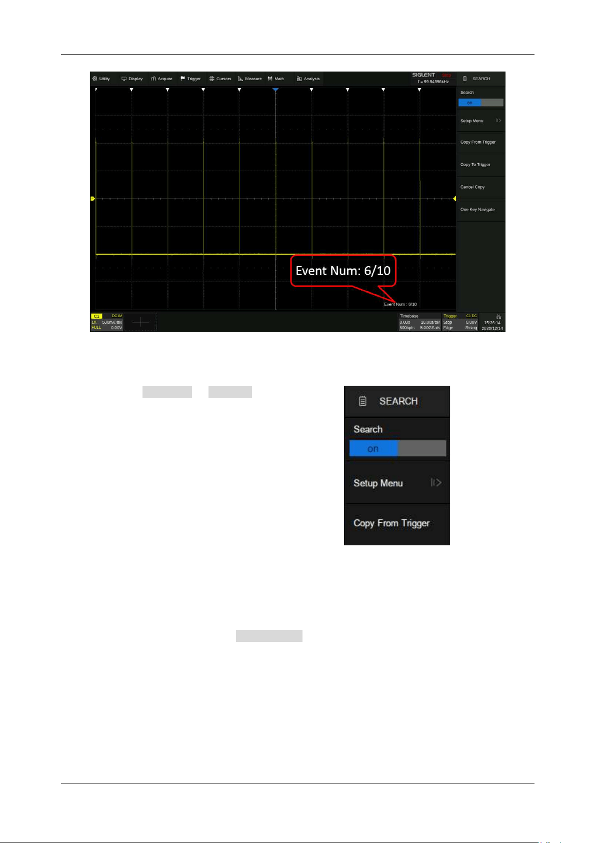
SDS6000L User Manual
int. s i g l e n t . c o m 2 0 5
Click the menu Analysis > Search to recall the
search dialog box and turn it on.
Setup Menu
Select and set the search type in the Setup Menu . The SDS6000L provides five search conditions:
Edge, Slope, Pulse, Interval, and Runt.
SDS6000L User Manual
2 0 6 i n t . s i g l e n t . c o m
Search Type
Setup Description
Edge
Slope: Rising, Falling, or Either
Slope
Slope: Rising, Falling
Limit Range setting is available
Pulse
Polarity: Positive, Negative
Limit Range setting is available
Interval
Slope: Rising, Falling
Limit Range setting is available
Runt
Polarity: Positive, Negative
Limit Range setting is available
Search setup is similar to the corresponding trigger type. See the sections “Edge Trigger”, “Slope
Trigger”, ”Pulse Trigger”, ”Interval Trigger” and ”Runt Trigger” for details.
Copy
The SDS6000L supports replication between search settings and trigger settings.
Copy from Trigger:
Synchronize the current trigger settings to the search settings.
Copy to Trigger:
Synchronize the current search settings to the trigger settings.
Cancel Copy:
Cancel the last synchronization and restore the settings before it.
Note:
When copying from the trigger, if the trigger type is not supported by
search, the operation is invalid.
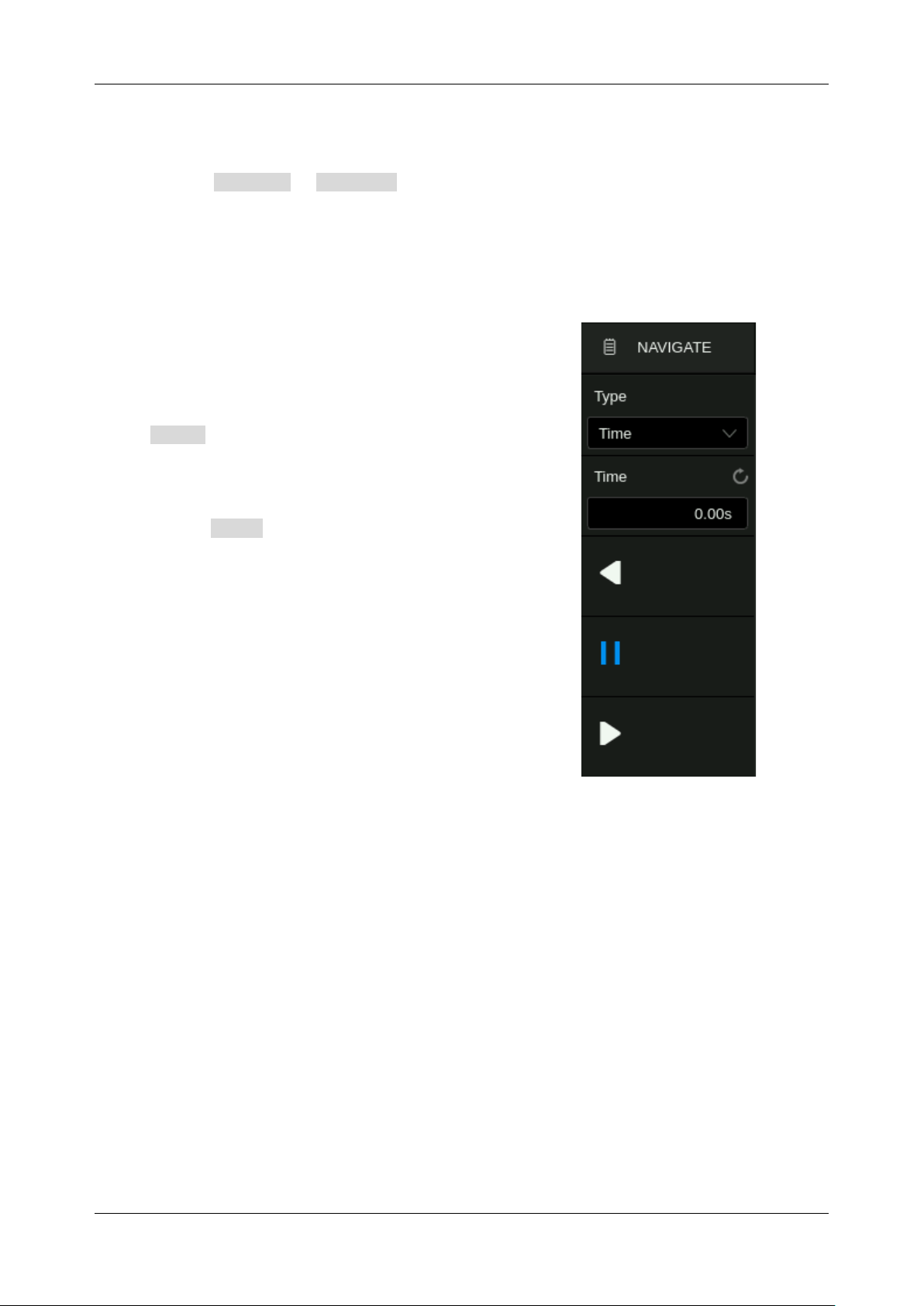
SDS6000L User Manual
int. s i g l e n t . c o m 2 0 7
21 Navigate
Click the menu Analysis > Navigate to recall the navigate dialog box. The SDS6000L provides
three navigate types: Search Event, Time, and History Frame.
Navigate by Time
The oscilloscope automatically adjusts the trigger delay
according to the direction set by the user.
Click Type in the navigate dialog box to select the
navigate type as “Time”. There are two ways to navigate
by time:
Click the Time area to set the time value by the
mouse wheel or the virtual keypad.
Click the navigation buttons
◀
, ||, or
▶
on the menu to
play backward, stop, or play forward the waveform.
Click the
◀
or
▶
buttons multiple times to speed up the
playing. Three replay speed levels are supported:
Low, Medium , and High Speed.
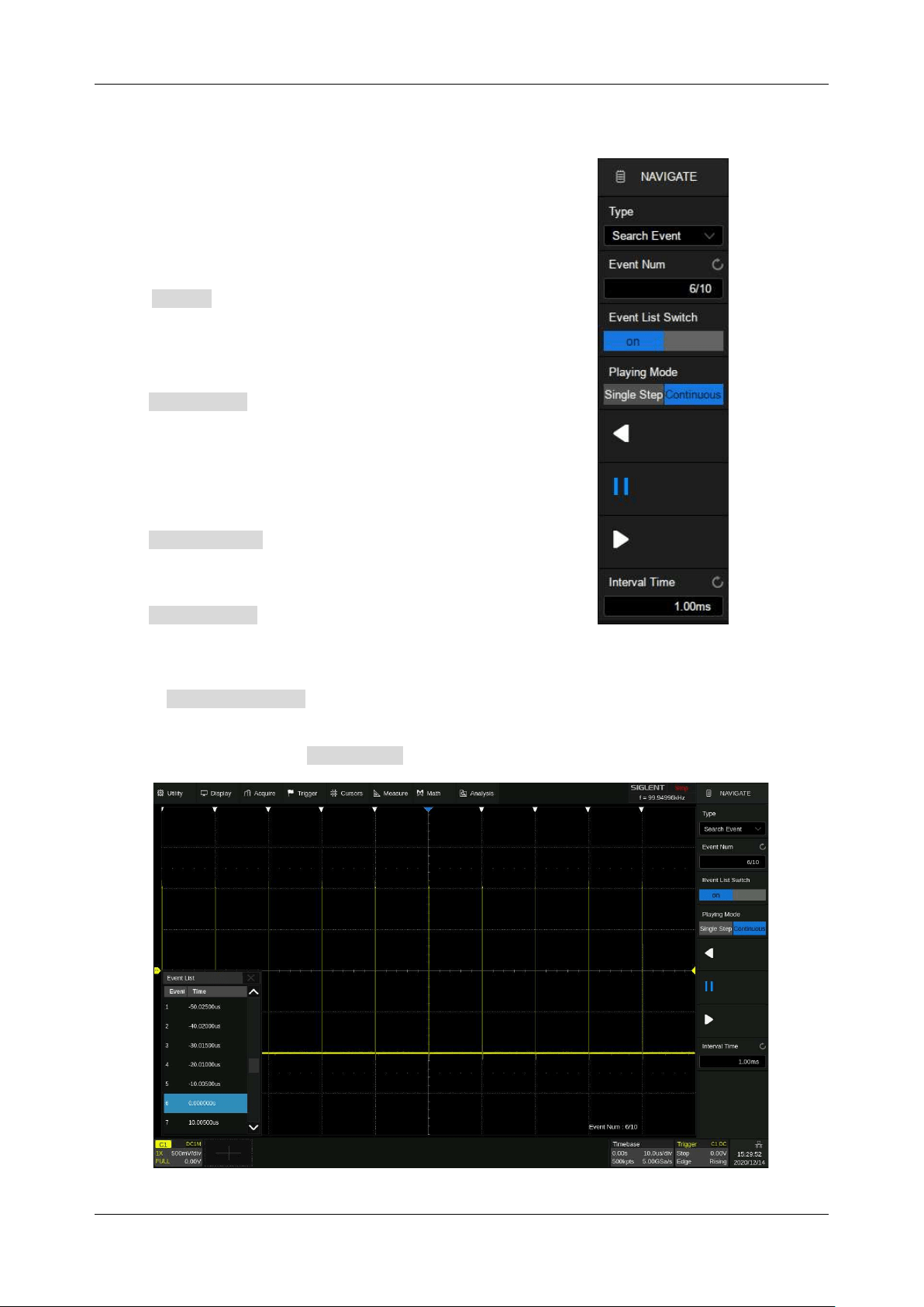
SDS6000L User Manual
2 0 8 i n t . s i g l e n t . c o m
Navigate by Search Event
When the Search function is turned on and the acquisition is
stopped, Navigate is usable to find search events (see the
chapter "Search" for the search function).
Click Type in the navigate dialog box to select the
navigate type as “Search Event”.
Click Event Num to set the event number by the mouse
wheel or the virtual keypad. Click the navigation buttons
◀
or
▶
on the front panel to go to the previous or next search event.
Click Playing Mode to set the search event playing mode.
Click Interval Time to set the playing interval by the mouse
wheel or the virtual keypad.
Click the Event List Switch area to turn the list on or off. The list contains time labels for each event.
Clicking a row in the list automatically jumps to the corresponding event. This operation is equivalent
to specifying an event in the Event Num area.
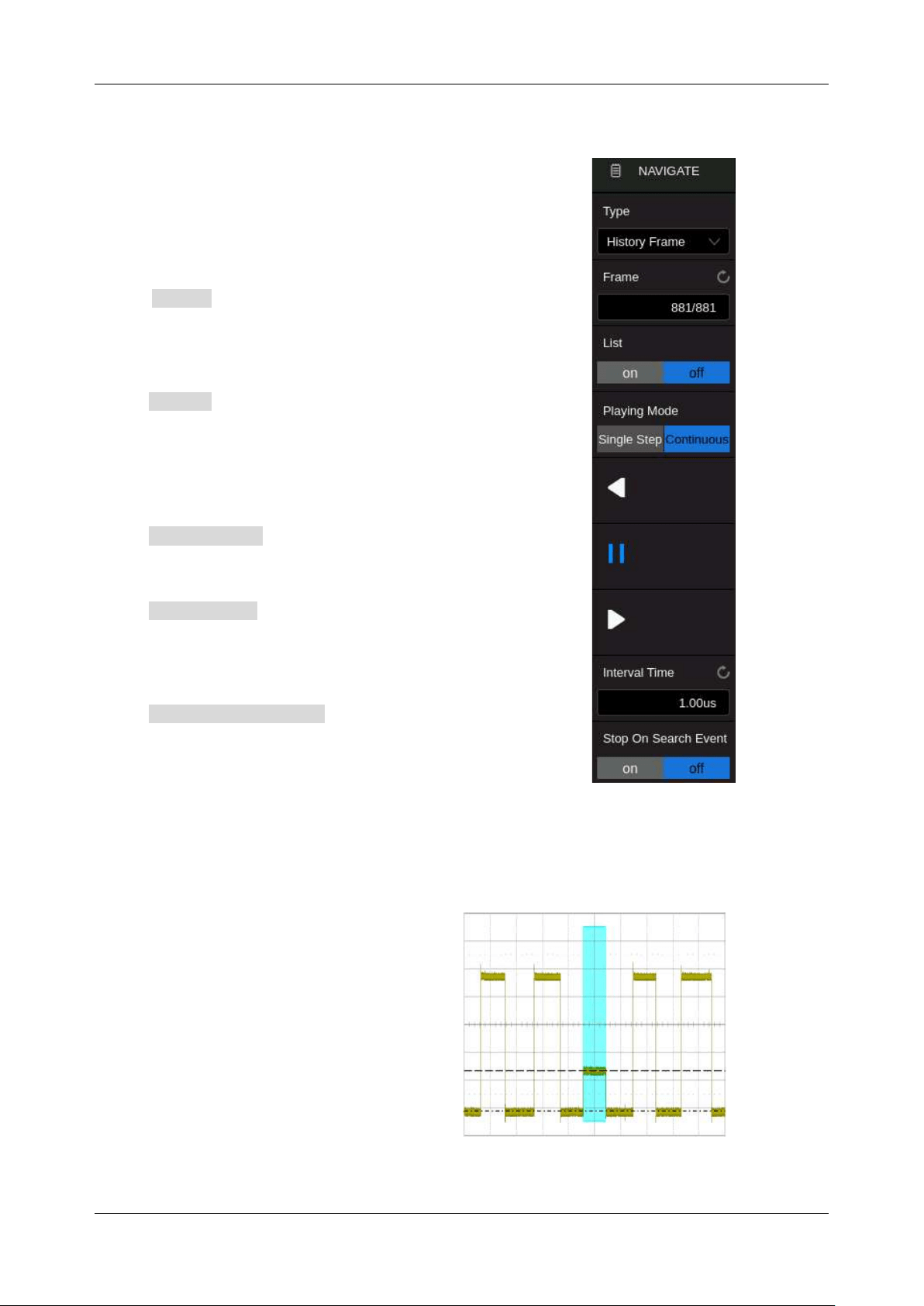
SDS6000L User Manual
int. s i g l e n t . c o m 2 0 9
Navigate by History Frame
When the history function is turned on, Navigate can be used
to play history frames (see the chapter "History" for details of
the history function).
Click Type in the navigate dialog box to select the
navigate type as “History Frame”.
Click Frame to set the frame number by the mouse wheel
or the virtual keypad. Click the navigation buttons
◀
, ||, or
▶
on
the menu to play backward, stop, or play forward.
Click Playing Mode to set the search event playing mode.
Click Interval Time to set the playing interval by the mouse
wheel or the virtual keypad.
Click Stop On Search Event to set the stop play condition:
stop when the event is searched. This setting is only valid
when the search function is on.
The following is an example of an occasional runt signal to demonstrate how to quickly locate and find
events of interest by using the combination of Search and Navigate:
The input signal is a 5 V periodic square
wave, in which every 200 ms there is a runt
pulse with a height of 1/3 of the normal
amplitude:
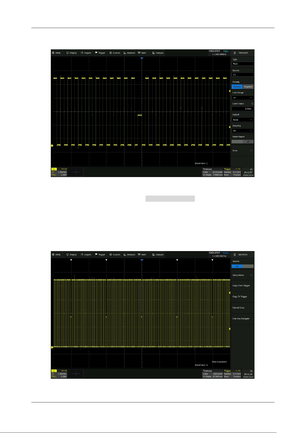
SDS6000L User Manual
2 1 0 i n t . s i g l e n t . c o m
First, set the trigger type to Runt to trigger on the runt pulse. See the section “Runt Trigger” for details.
Then turn on the Search function and operate Copy from Trigger in the search dialog box so that
the oscilloscope searches for the dwarf pulses according to the same setting as the trigger.
Set the horizontal scale to 100 ms/div, then 5 markers with ~200 ms interval are shown on the display,
indicating that a total of 5 dwarf pulses were found in the full screen of 1 second time range:
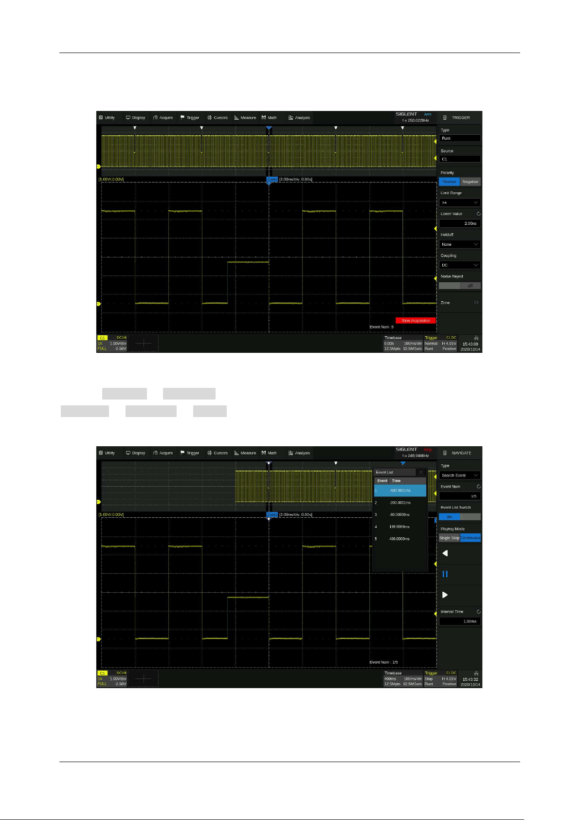
SDS6000L User Manual
int. s i g l e n t . c o m 2 11
Turn on the Zoom function to observe the full view of the frame and the detail of the third dwarf pulse
at the same time:
Perform Acquire > Run/Stop to stop the acquisition, and then follow the steps
Analysis > Navigate > Type to select “Search Event”. The following figure shows the first
dwarf pulse. In this example, the list is enabled and the time labels of each event are shown in the list.
SDS6000L User Manual
2 1 2 i n t . s i g l e n t . c o m
22 Mask Test
22.1 Overview
Users can create masks and define the rule used to evaluate Pass/Fail operations. An event violating
the rule is defined as a failure and a pulse can be generated from the "
Aux Out
" port on the back panel.
This is very useful to find and quantify anomalies in production tests or similar batch measurements.
When Pass/Fail is enabled, the signal output from the
Aux Out
is automatically switched to Pass/Fail
pulse.
A. Mask area in green. Any dot violating the rule is highlighted in red, instead of the normal
waveform color.
B. Pass/Fail information display area, including the count of the passed frames, failed frames,
total frames, and the fail rate.
C. Dialog box
SDS6000L User Manual
int. s i g l e n t . c o m 2 1 3
Perform Analysis > Mask Test to open the Mask Test dialog box:
A. Turn on/off the test
B. Select the source
(
C1~C8
)
C. Select the rule
(
All In, All Out, Any In, and Any Out
)
D. Set the mask
E. Change the state of the Pass/Fail operation. Turning
off the operation when the test is in progress will stop
the test immediately, and the counters in the
information display area will stop. Turning the test
back on will re-start the test and clear the counters.
F. Turn on/off the information display
G. Turn on/off “Stop on Fail”. When it is "on", the
oscilloscope stops the acquisition once it detects a
failure
H. Turn on/off “Failure to History”. When it is "on", the
failure frame will be stored internally and can be
viewed through the history function
I. Turn on/off “Capture on Fail”. When it is "on", the
failure waveform is detected, and the screenshot with
the failure frame will be stored in the external U disk.
J. Turn on/off the sound prompt when a failure occurs.
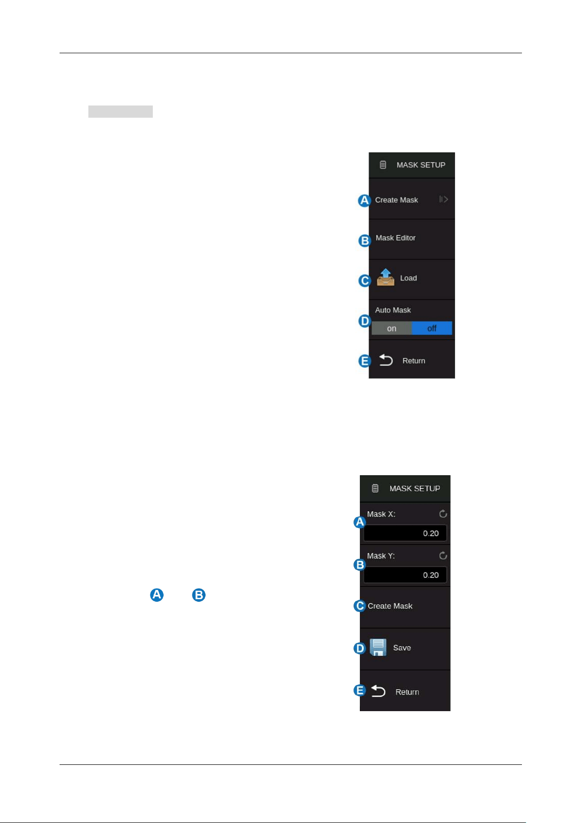
SDS6000L User Manual
2 1 4 i n t . s i g l e n t . c o m
22.2 Mask Setup
Click Mask Setup in the Mask Test dialog box to set the mask. There are two methods to create a
mask, one is by setting horizontal and vertical values, and the other is by drawing a polygon mask.
A. Create a mask automatically according to
the waveform
B. Create a custom mask using the Mask
Editor tool
C. Load the mask
D. When “Auto Mask” is On, the mask grows
or shrinks in proportion to the horizontal or
vertical setting values. As they change, the
mask adjusts to fit the new scaling values
E. Return to the previous menu
22.2.1 Create Mask
The mask can be created based on an existing waveform trace.
A. Set the spacing of the mask to the trace
horizontal. The units are parts of the
horizontal division setting.
B. Set the spacing of the mask to the trace
vertical. The units are parts of the vertical
division setting. Create the mask based on
settings in and
C. Save the mask
D. Return to the previous menu
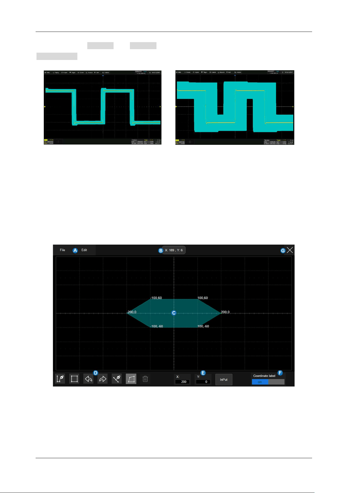
SDS6000L User Manual
int. s i g l e n t . c o m 2 1 5
Set the values for Mask X and Mask Y (in divisions of the display graticule), and then perform
Create Mask to generate the mask. The horizontal and vertical adjustment range is 0.08~4.00 div.
X = 0.2 div, Y = 0.2 div
X = 1 div, Y = 1 div
Saving and recalling mask files (*.msk) is similar to the operation of setup files, see the chapter
"Save/Recall" for details.
22.2.2 Mask Editor
The Mask Editor is a built-in tool that provides an approach to create custom masks. Below is its layout:
A. Menu bar
B. Coordinate the latest selected point on the display
C. Mask edit area, which is equivalent to the grid area. In this example, a hexagon has been
created as a part of the mask
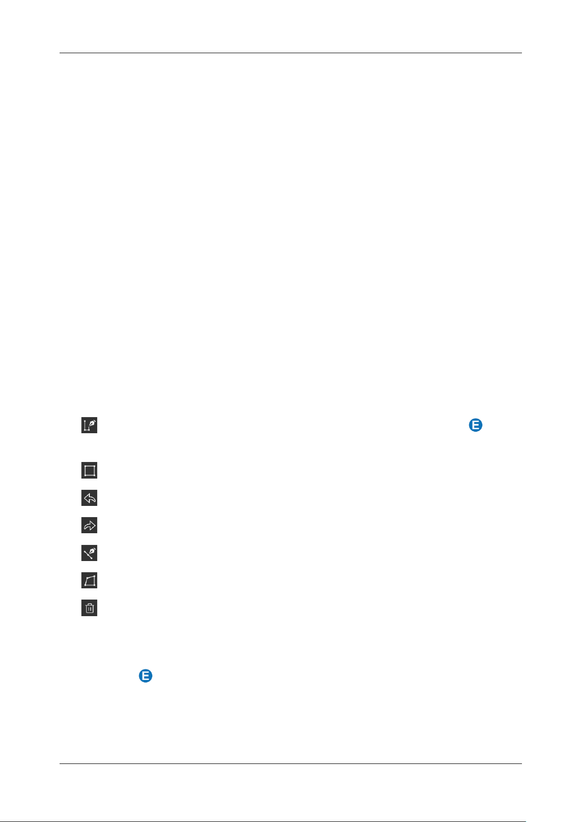
SDS6000L User Manual
2 1 6 i n t . s i g l e n t . c o m
D. Toolbar
E. Coordinate edit area. Set the X ordinate and Y ordinate by the virtual keypad and then click
the “Input” button the perform the ordinate update
F. Display or hide the coordinates of the polygon vertices on the display
G. Exit the tool
Menu bar
There are 2 menus on the menu bar. The File menu includes ordinary file operations such as:
New:
Create a new mask file
Open:
Open an existing mask file
Save:
Save the current mask file
Exit:
Exit the Mask Editor tool
The contents of the Edit menu are equivalent to the Toolbar.
Toolbar
Draw:
Creates vertices of a polygon by clicking the display or entering values in
coordinate edit area
Create Polygon:
Creates a polygon based on the drawn vertices by the operation Draw
Undo
Redo
Insert Point:
Inserts a vertex on a selected side
Edit Polygon:
Edits a polygon. Vertices, sides, and the polygon are all editable object
Delete Polygon:
Deletes selected polygon
To edit a vertex, side, or polygon object, first select it, and then move it by mouse or by entering the
desired value in coordinate edit area. For a side, the value is for its middle point. For a polygon,
the ordinate is for its geometric center.
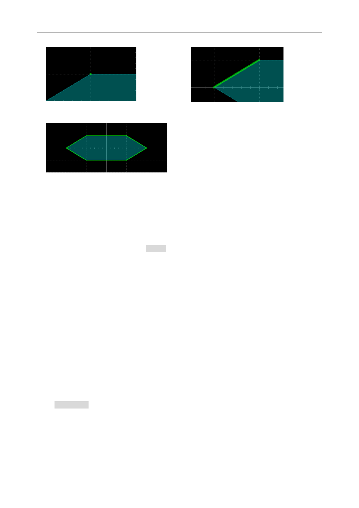
SDS6000L User Manual
int. s i g l e n t . c o m 2 1 7
Select a vertex (point)
Select a side (line segment)
Select a polygon
22.3 Pass/Fail Rule
The Pass / Fail rule is specified at the Type region in the Mask Test dialog box.
All In:
All data points must be inside the mask to pass the test. Even a single point outside
the mask will cause a failure.
All Out:
All data points must be outside the mask to pass the test. Even a single point inside
the mask will cause a failure.
Any In:
Any data point inside the mask will be recognized as a pass. All data points outside
the mask will cause a failure.
Any Out:
Any data point outside the mask will be recognized as a pass. All data points inside
the mask will cause a failure.
22.4 Operation
Click Operation to start / stop the test. Stopping a test in progress and restarting the test will clear
the count of the passing frames, failed frames, total frames, and the fail rate.
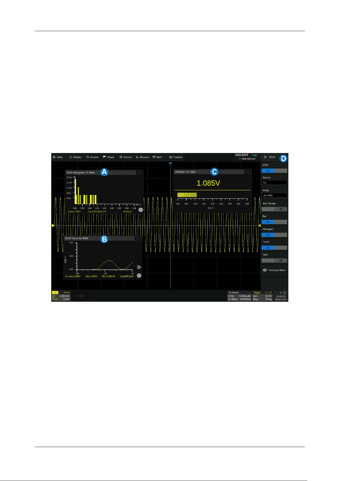
SDS6000L User Manual
2 1 8 i n t . s i g l e n t . c o m
23 DVM
23.1 Overview
The DVM (Digital Voltage Meter) function can be used to measure parameters such as DC and AC
amplitudes. The SDS6000L measures the specified parameter of the input signal and can display it in
various formats, including Bar, Histogram, and Trend. DVM is asynchronous to the acquisition system
of the oscilloscope. Sources of DVM and Measurement can be different, and DVM can work well even
if the acquisition of the oscilloscope is stopped.
A. Histogram display area
B. Trend display area
C. Bar display area
D. DVM dialog box
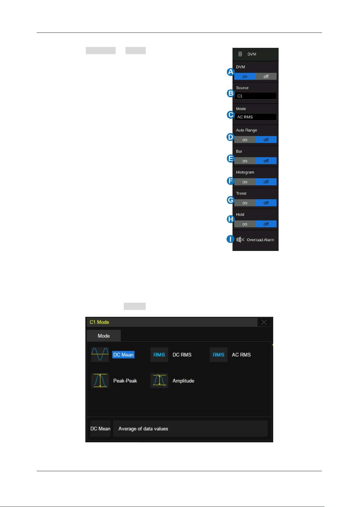
SDS6000L User Manual
int. s i g l e n t . c o m 2 1 9
Click the menu Analysis > DVM to open the
DVM dialog box:
A. Turn on or off the DVM
B. Select the source (C1~C8)
C. Select the Mode: DC Mean, DC RMS, AC
RMS, Peak-Peak, and Amplitude
D. Turn on or off the Auto Range
E. Turn on or off the bar diagram
F. Turn on or off the histogram diagram
G. Turn on or off the trend plot
H. Turn on or off Hold. DVM stops
acquisition in Hold mode
I. Turn on the overload alarm, an alarm will
sound when the signal is out of range
23.2 Mode
DVM provides 5 modes. Click mode in the DVM dialog box to open the mode selection window:
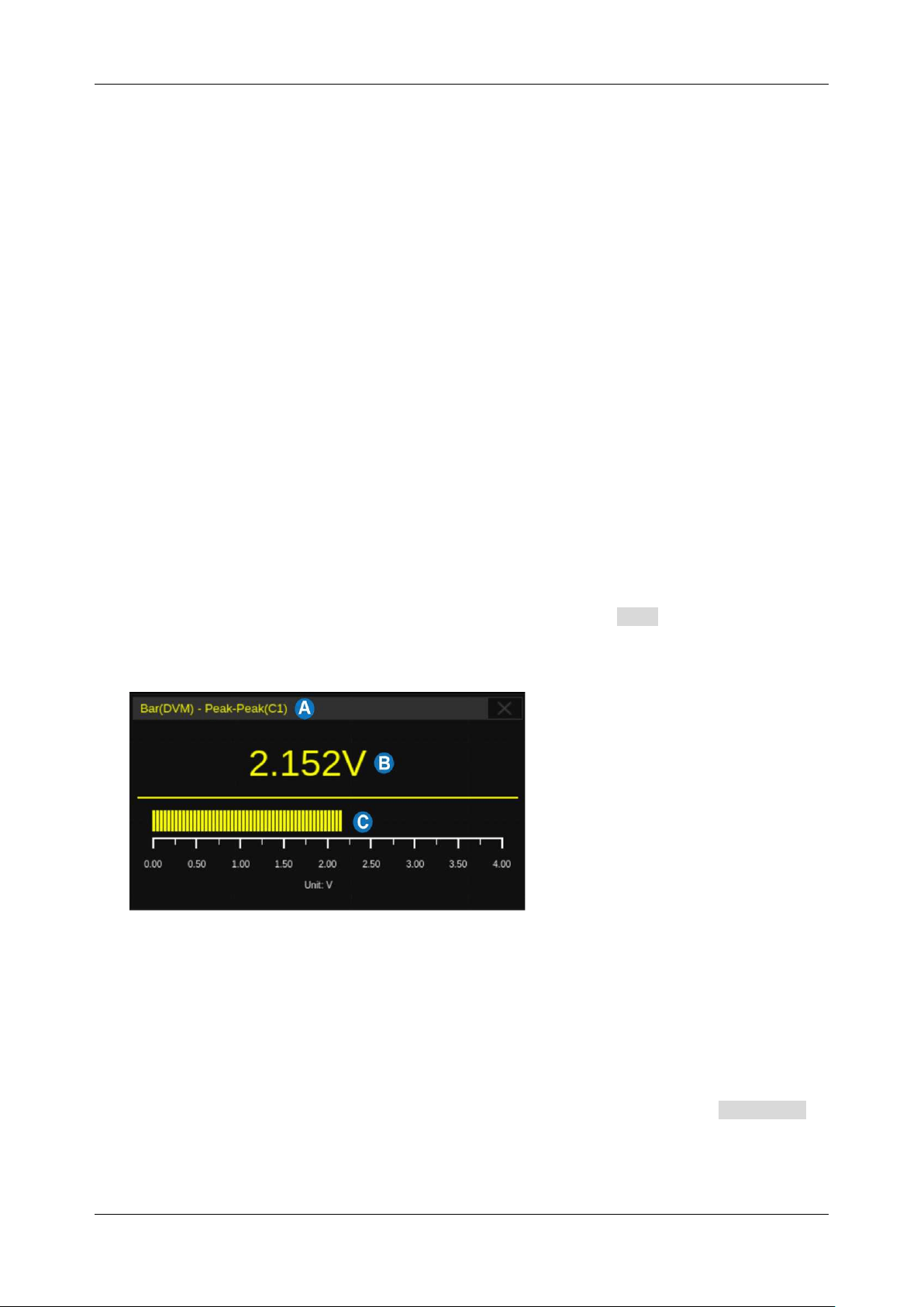
SDS6000L User Manual
2 2 0 i n t . s i g l e n t . c o m
DC Mean:
Average of the data
DC RMS:
Root mean square of the data at DC coupling
AC RMS:
Root mean square of the data at AC coupling
Peak-Peak:
Difference between maximum and minimum data value
Amplitude:
Difference between top and base in a bimodal waveform. If not bimodal, the difference
between max and min.
23.3 Diagrams
After selecting the mode, users can click the screen to open the state diagrams: bar, histogram, and
trend. The color of the data in the diagrams is consistent with the color of the source.
Bar
The bar diagram accurately displays the current measured value. Click Bar in the DVM dialog box
to display it.
A. Mode
B. Current value
C. Bar corresponding to the current value
Histogram
A histogram visually indicates the probability distribution of the measured values. Click histogram in
the DVM dialog box to display it.
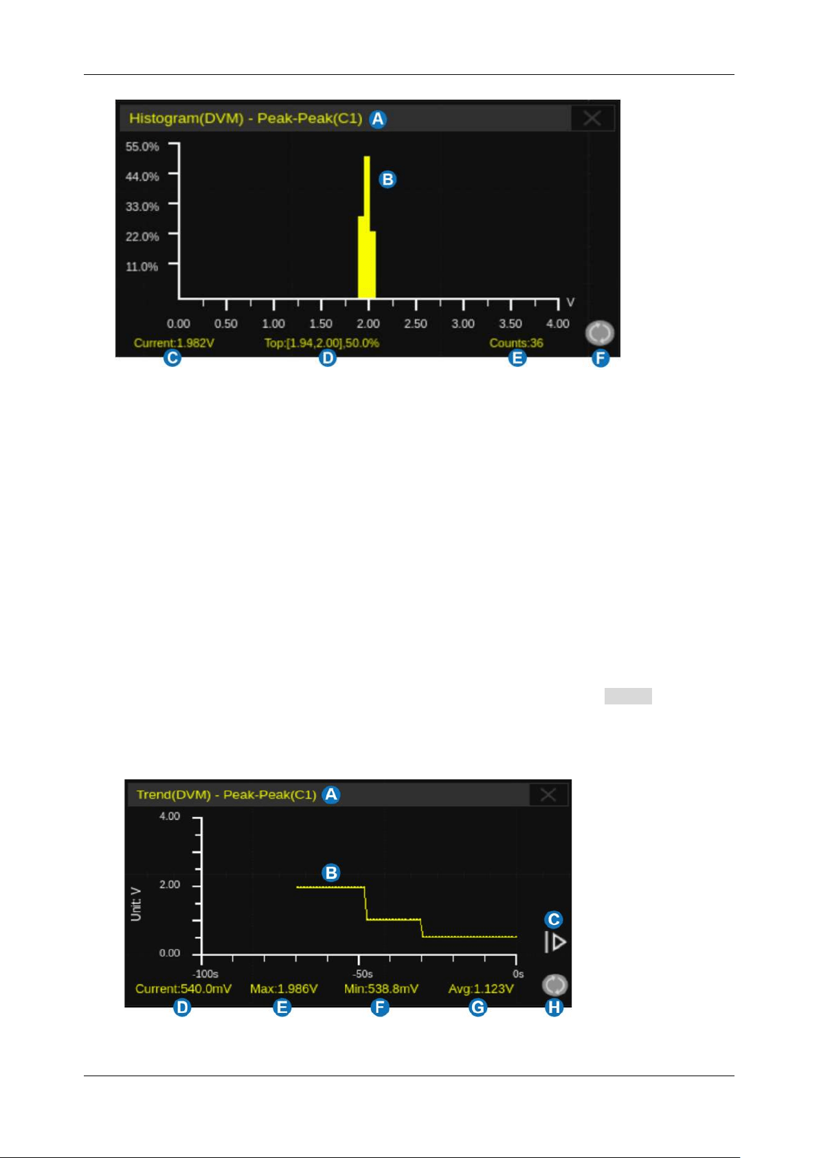
SDS6000L User Manual
int. s i g l e n t . c o m 2 2 1
A. Mode
B. Histogram display area
C. Current value
D. The bin includes the maximum value and probability with which values fall into it
E. Statistics counts
F. Reset statistics
Trend
The trend diagram indicates the trend of the measured values over time. Click trend in the DVM
dialog box to display it.
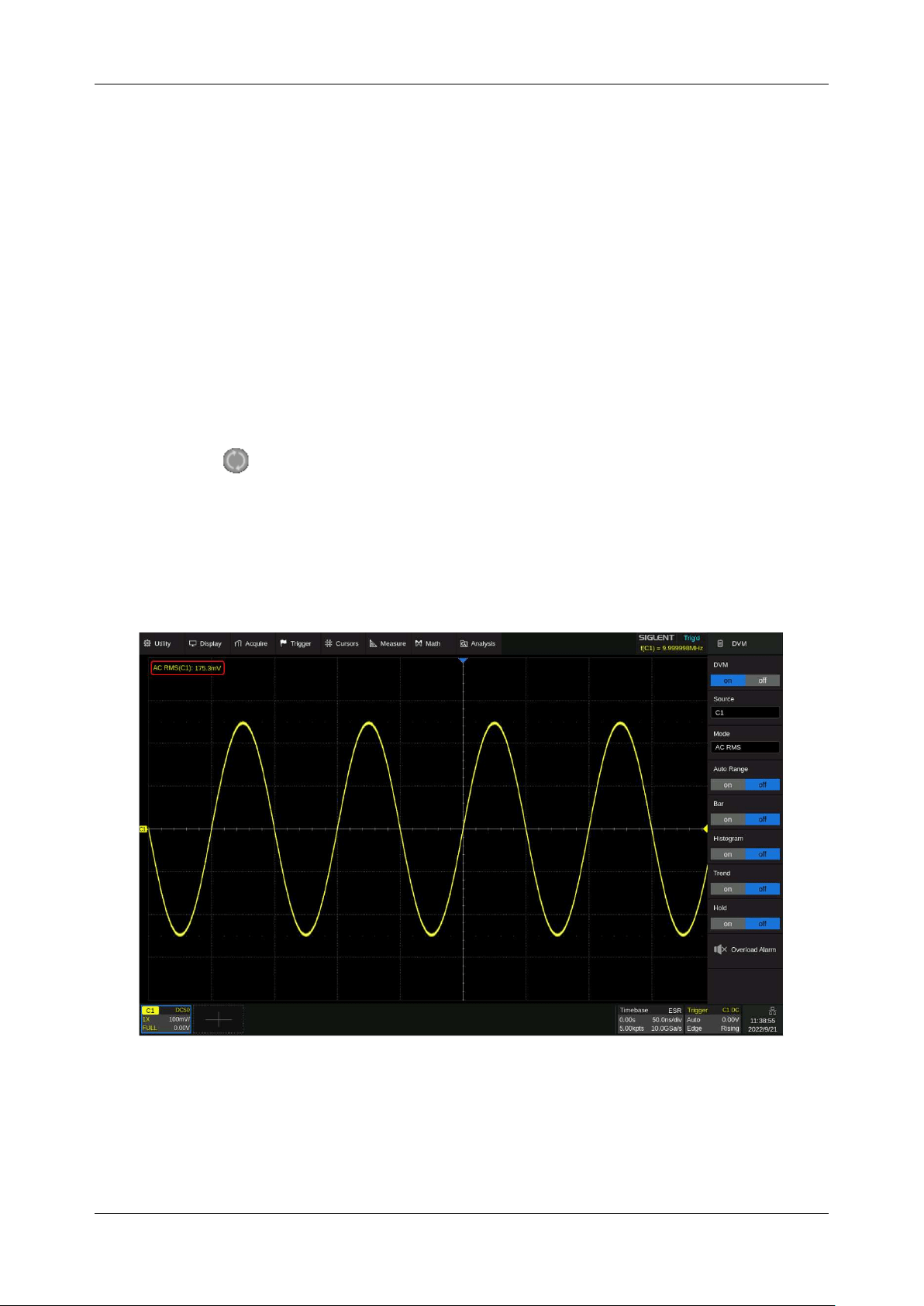
SDS6000L User Manual
2 2 2 i n t . s i g l e n t . c o m
A. Mode
B. Trend display area
C. Extend the range of time. Click it to expand the time range.
D. Current value
E. Maximum value
F. Minimum value
G. Average value
H. Reset statistics
Click the symbol in the histogram and trend display areas to restart statistics.
When all the 3 diagrams are closed, there is a simple information bar on the top-left of the waveform
display area to show the current value of the DVM:
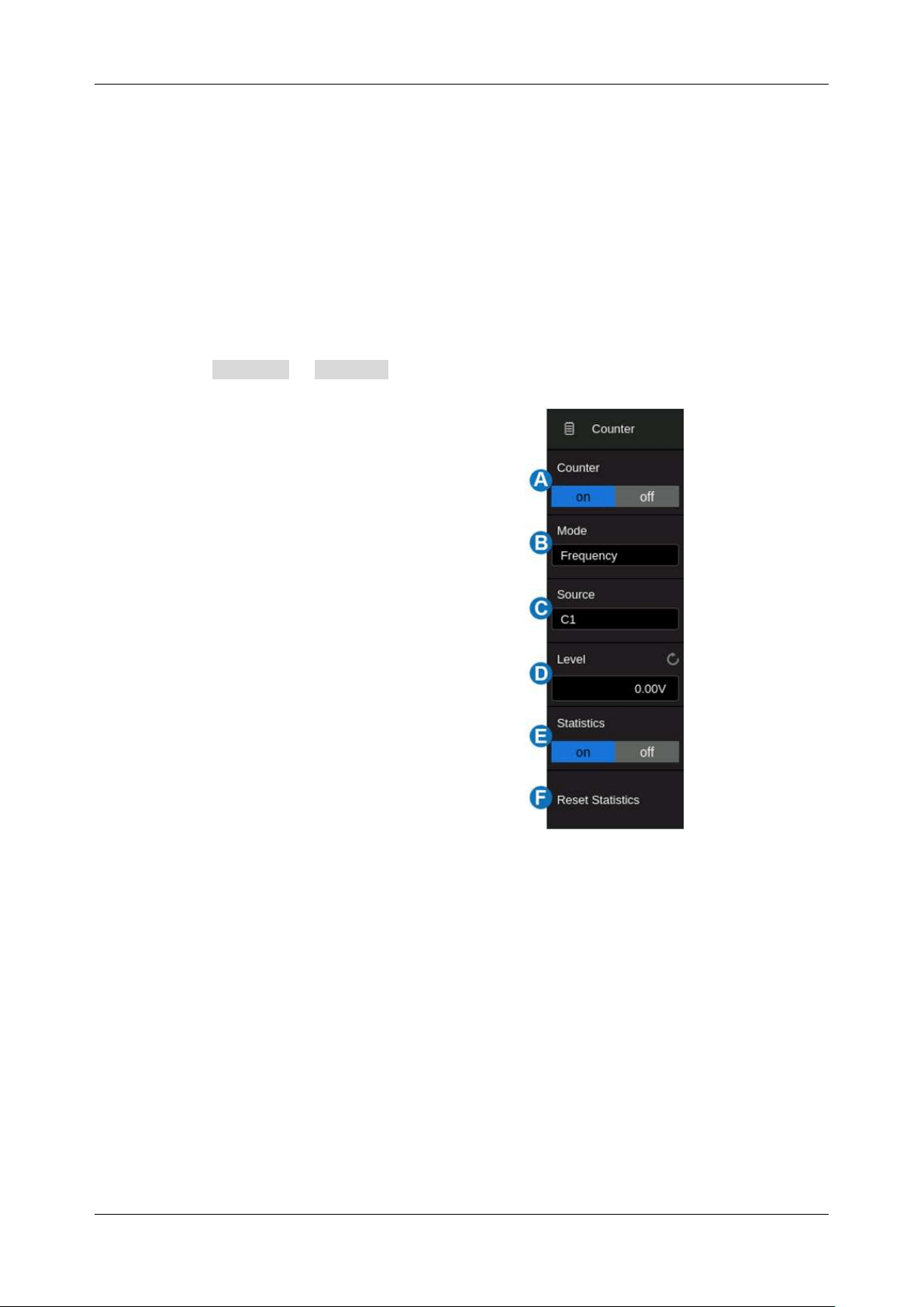
SDS6000L User Manual
int. s i g l e n t . c o m 2 2 3
24 Counter
24.1 Overview
The counter is used to measure the frequency and period of a signal or count the events happening
within it. The counter is asynchronous to the acquisition system of the oscilloscope. It can work well
even if the acquisition of the oscilloscope is stopped.
Click the menu Analysis > Counter to open the counter dialog box:
A. Turn on or off Counter
B. Select the mode: frequency,
period, and totalizer
C. Select the source (C1~C8)
D. Set the level of the counter
E. Turn on or off statistics
F. Clear and restart the statistics.
Mode
See the section “Mode” for details.
Statistics
When statistics are enabled, the counter will increment the data and display the statistics results on
the screen.

SDS6000L User Manual
2 2 4 i n t . s i g l e n t . c o m
Value
– The latest count
Mean
– The average of all historical counts
Min
– The minimum of all historical counts
Max
– The maximum of all historical counts
Stdev
– The standard deviation of all historical counts, used to judge the distribution of historical count
parameters
Count
– Number of counts obtained
Level
– Counter level
Click Reset Statistics in the measure dialog box to clear and restart statistics.
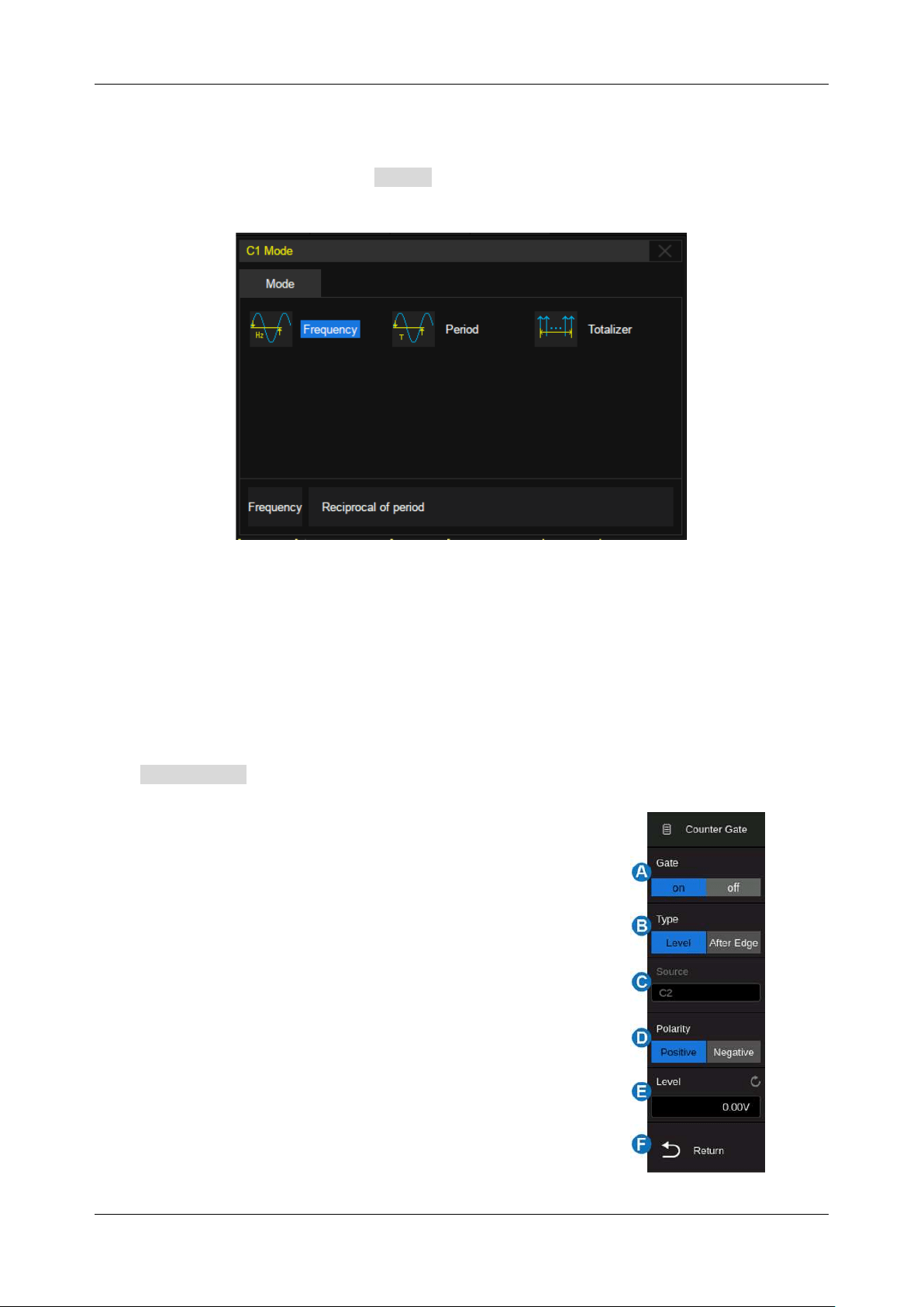
SDS6000L User Manual
int. s i g l e n t . c o m 2 2 5
24.2 Mode
The counter provides 3 modes. Click mode in the counter dialog box to open the mode selection
window:
Frequency:
Average frequency over a set period
Period:
The reciprocal of the average frequency over a set period
Totalizer:
Cumulative count
When the mode is set to totalizer, the edge of the counting source needs to be set. When the counting
gate is turned on, the counter can count only when the gate-source meets the specified conditions.
Click Gate Setting to recall the gate setting dialog box:
A. Turn on or off the gate
B. Select the gate type: Level or After Edge
C. Gate source display area. C1 and C2 are gate sources of
each other, C3 and C4 are gate sources of each other, C5
and C6 are gate sources of each other, C7 and C8 are gate
sources of each other
D. When the gate type is level, set the polarity (Positive or
Negative) of the gate source. When the gate type is edge,
set the slope (Rising or Falling edge) of the gate source.
E. Set the gate level
F. Return to the previous menu
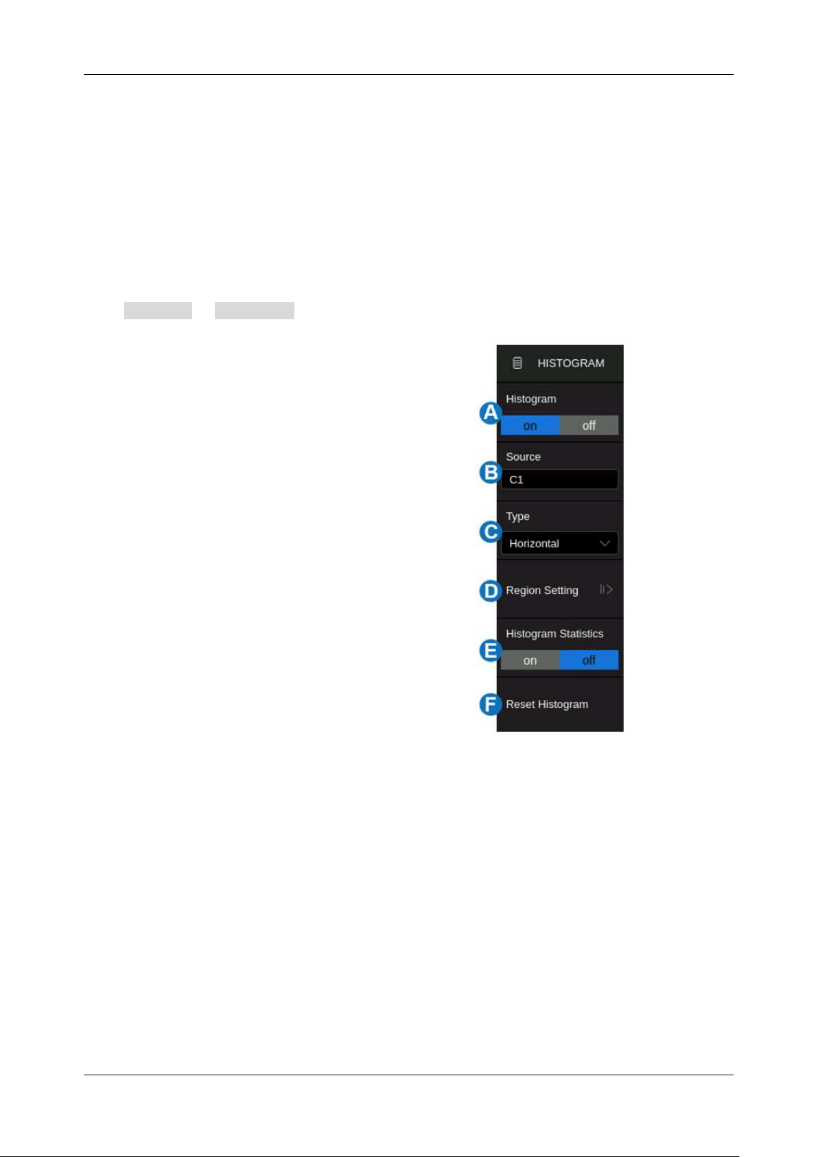
SDS6000L User Manual
2 2 6 i n t . s i g l e n t . c o m
25 Histogram
25.1 Overview
The SDS6000L supports waveform histograms for observing probability distributions of the waveform
in the specified region. The statistics can be performed in both horizontal and vertical directions. The
histogram continues to update as long as the acquisition is active.
Click Analysis > Histogram to recall the Histogram dialog box:
A. Turn on or off the histogram
B. Select the source of the histogram:
C1~C8. When Zoom is turned on, the
source selection is automatically
switched to Z1-Z8
C. Set the type of histogram: Horizontal,
Vertical or Both
D. Set the region of the histogram. The
setting range is within the waveform
area.
E. Turn on or off histogram statistics
F. Clear and restart the histogram
statistics.
Type
Horizontal – Displays the histogram in the horizontal direction. The oscilloscope counts waveform
data falling into every horizontal (time) bin defined by the histogram region and shows the
histogram at the bottom of the waveform area.
Vertical – Displays histogram in the vertical direction. The oscilloscope counts waveform data
falling into every vertical (amplitude) bin defined by the histogram region and shows the histogram
at the left of the waveform area.
Both – Displays both horizontal and vertical histograms
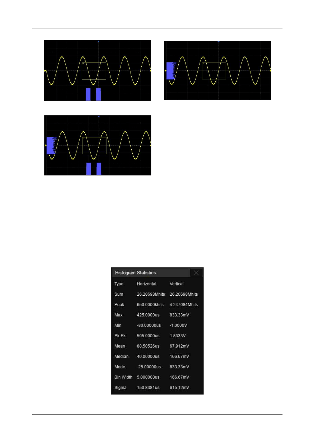
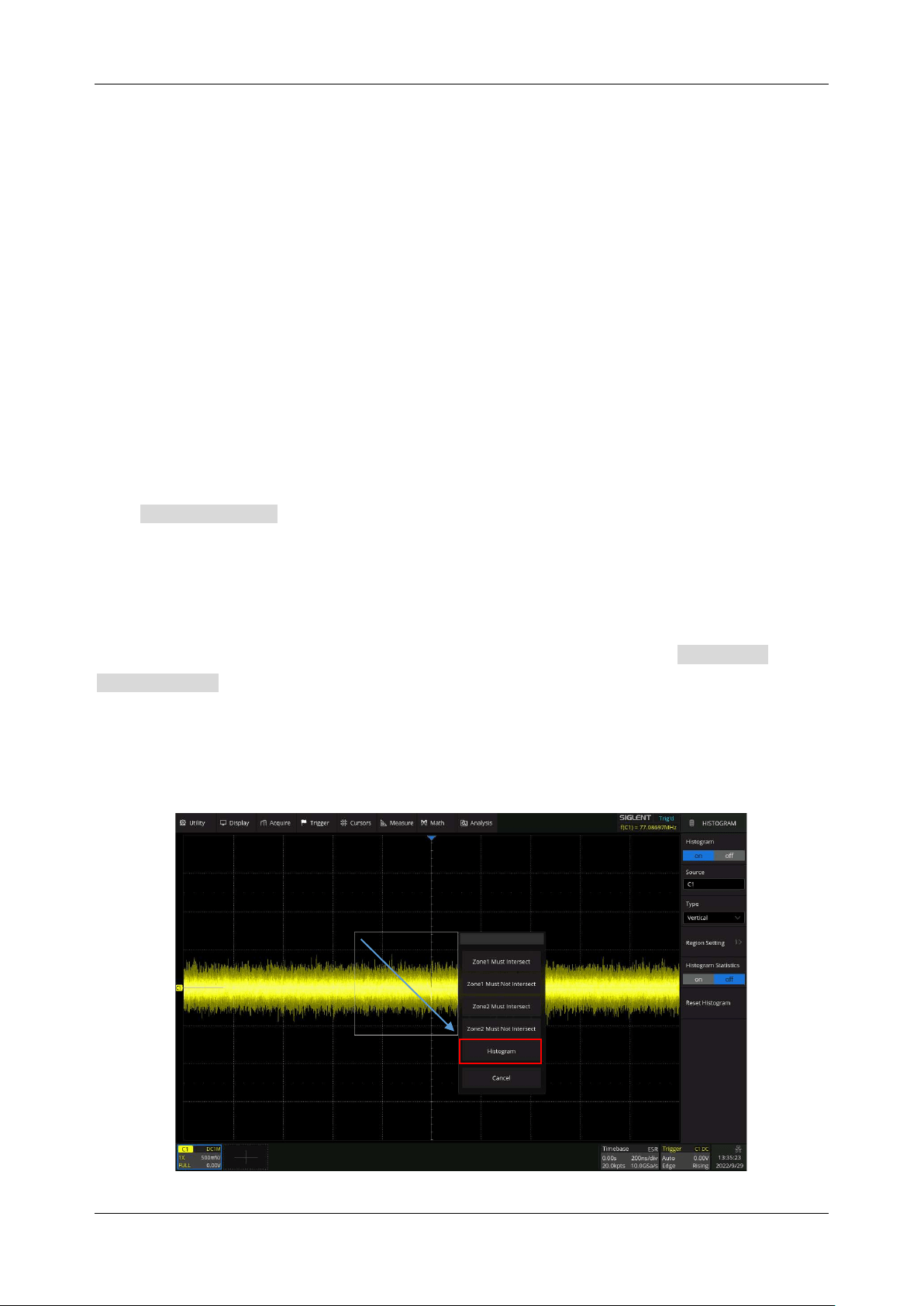
SDS6000L User Manual
2 2 8 i n t . s i g l e n t . c o m
Sum
– Total samples falling in the histogram region
Peak
– Samples in the highest bin
Max
– Maximum value of the samples
Min
– Minimum value of the samples
Pk-Pk
– Maximum - Minimum
Mean
– Mathematical expectation (or average) value of the samples
Median
– The value separating the higher half from the lower half of the histogram
Mode
– The value that appears most often
Bin Width
– The width of each bin
Sigma
– Standard deviation of the samples
Click Reset Histogram in the histogram dialog box to clear and restart the statistics.
25.2 Region Setting
Histogram region can be created and moved directly by the mouse or by setting Histogram >
Region Setting in the dialog box. The border color of the histogram region is consistent with the color
of the specified source.
By the mouse
Click any position of the waveform area and draw a rectangular box, as follow:
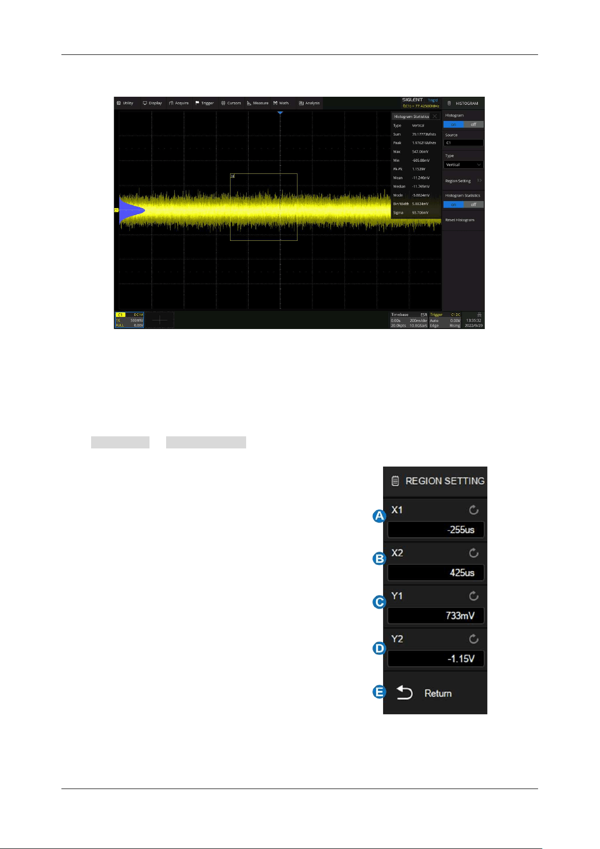
SDS6000L User Manual
int. s i g l e n t . c o m 2 2 9
A menu pops up at the end of the drawing action. Select "Histogram" in the menu:
After the region is created, it can be moved by dragging action.
Dialog Box
Click Histogram > Region Setting to recall the dialog box.
A. Set the left border of the histogram region
B. Set the right border of the histogram region
C. Set the top border of the histogram region
D. Set the bottom border of the histogram region
E. Return to the previous menu
Click the area above to set the value by the mouse wheel
or the virtual keypad.
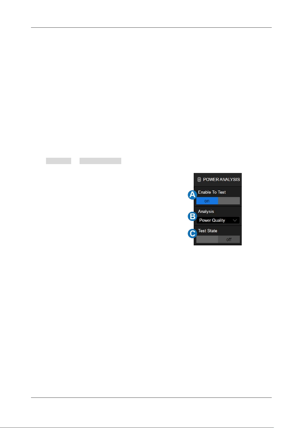
SDS6000L User Manual
2 3 0 i n t . s i g l e n t . c o m
26 Power Analysis
26.1 Overview
The SDS6000L supports a power analysis function. Power analysis can help users quickly and easily
analyze and debug switching power supply design. It automatically calculates Power Quality, Current
Harmonics, Inrush Current, Switching Loss, Slew Rate, Modulation, Turn On/Turn Off, Transient
Response, PSRR, Power Efficiency, Output Ripple, etc. Full use of the Power analysis requires a
differential voltage probe like the SIGLENT DPB series, a current probe like the SIGLENT CP series,
the SIGLENT DF2001A deskew fixture, and the power analysis activation license (part number
SDS6000L-PA). Install the software option part number SDS6000L-PA to permanently enable the
power analysis function.
Click Analysis > Power Analysis to recall the power analysis dialog box:
A. Enable/Disable the test
B. Select the analysis item (Power Quality,
Current Harmonics, Inrush Current, Switching
Loss, Slew Rate, Modulation, Turn On/Turn
Off, Transient Response, PSRR, Power
Efficiency, Output Ripple, etc.)
C. Turn on/off the state of the analysis item
26.2 Power Quality
The specific measurement parameters of power quality analysis include active power, apparent power,
reactive power, power factor, power phase angle, voltage effective value, current effective value,
voltage crest factor, and current crest factor of power input of a switching power supply.
Type
Power
-- Includes all the items to describe energy flow in a system: Active power, reactive power,
apparent power, power factor, and power phase angle.

SDS6000L User Manual
int. s i g l e n t . c o m 2 3 1
P: Active Power =
S: Apparent Power = Vrms * Irms
Q: Reactive Power =
Power Phase Angle: Phase difference between voltage and current
Power Factor, which is the ratio of active power and apparent power.
Voltage Crest
-- Voltage parameters of the power input include voltage crest, voltage effective value,
and voltage crest factor.
Vrms =
V_Crest = Vpeak / Vrms
Current Crest
-- Current parameters of the power input include current crest, current effective value,
and current crest factor.
Irms =
I_Crest = Ipeak / Irms
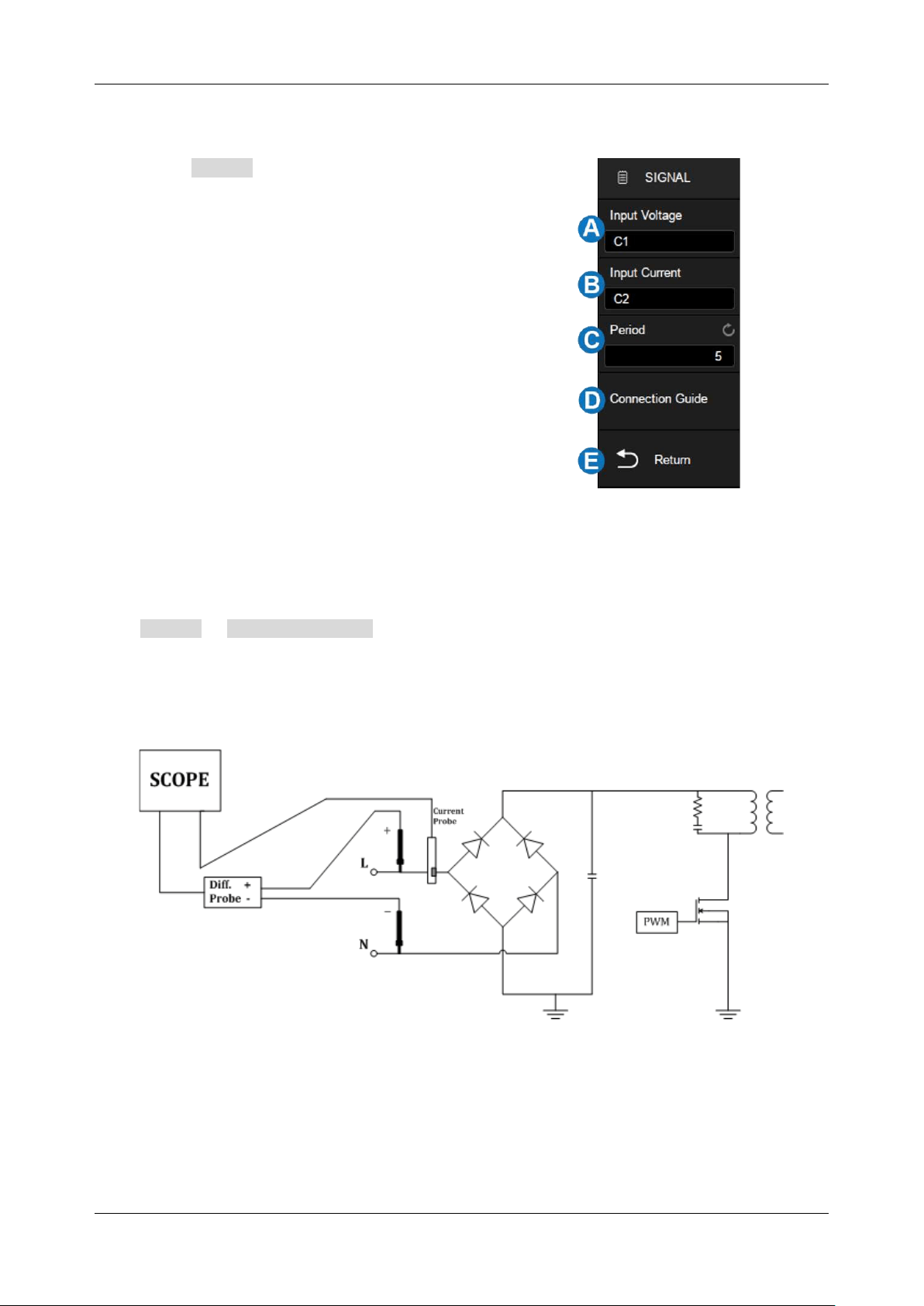
SDS6000L User Manual
2 3 2 i n t . s i g l e n t . c o m
Signal Settings
Click Signal to recall signal settings dialog box:
A. Set the input voltage source
B. Set the input current source
C. Set the periods displayed
D. View the connection guide
E. Return to the previous menu
Connection Guide
Click Signal > Connection Guide to recall the connection guide of power quality, as shown in the
figure below. Please follow the instructions in this figure for correct connections. Click the icon on the
top right of the guide to close.
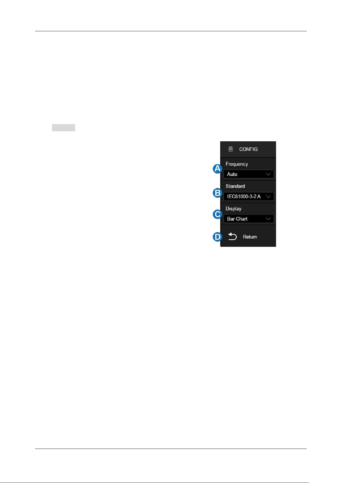
SDS6000L User Manual
int. s i g l e n t . c o m 2 3 3
26.3 Current Harmonics
Current harmonics are used to analyze the input current harmonics. An FFT of the selected channel is
performed to get the harmonic components. The signal settings and connection guide are the same as
the power quality test.
Configuration
Click Config to recall the configuration dialog box:
A. Set the frequency of the line (Auto, 50 Hz,
60 Hz, or 400 Hz)
B. Set the standard type (IEC61000-3-2 A,
IEC61000-3-2 B, IEC61000-3-2 C or
IEC61000-3-2 D)
C. Set the display type (Off, Bar Chart, or Table)
D. Return to the previous menu
Standard
IEC 61000-3-2 is an international standard that limits mains voltage distortion by prescribing the
maximum value for harmonic currents from the second harmonic up to and including the 40th harmonic
current. There are 4 different classes in the EN 61000-3-2 that have different limit values:
Class A: Balanced 3-phase equipment, household appliances excluding equipment identified as
class D, tools, excluding portable tools, dimmers for incandescent lamps, audio equipment, and
all other equipment, except that stated in one of the following classes.
Class B: Portable tools, arc welding equipment which is not professional equipment
Class C: Lighting equipment.
Class D: PC, PC monitors, radio, or TV receivers. Input power P ≤ 600 W.I
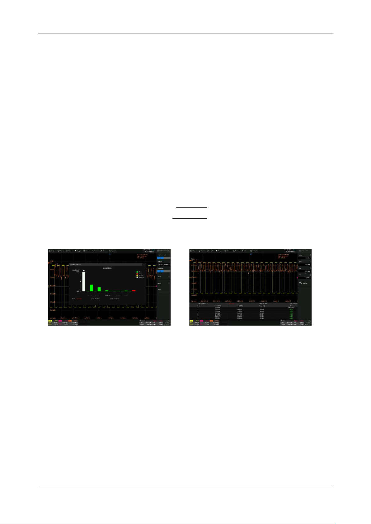
SDS6000L User Manual
2 3 4 i n t . s i g l e n t . c o m
Parameter Description
For the first 40 harmonics, the following values are displayed:
Measured Value (RMS)
-- The measured value displayed in the unit specified by the harmonic unit
parameter
Limit Value (RMS)
-- Limits specified by the selected standard
Margin (%)
--The margin specified by selected standard parameters. The margin value is (standard
value - measured value) / standard value * 100%
Pass/Fail State
-- Determine whether the measured value is passed or failed according to the selected
standard. The rows in the table or the bars in the bar chart are rendered in different colors based on
the pass / fail state. When the value is greater than 85% of the limit but less than 100% of the limit, it
is defined as a critical state.
Total Harmonic Distortion
(
THD
)
=
,
where X
n
is the nth harmonic, and X
1
is
the basic component.
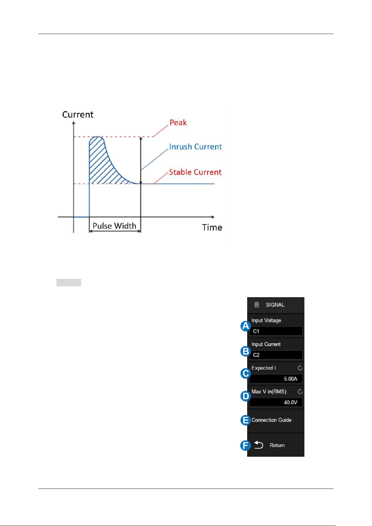
SDS6000L User Manual
int. s i g l e n t . c o m 2 3 5
26.4 Inrush Current
A large current far greater than the stable current may flow through at the moment of switching on a
power supply. The large current is called the inrush current. The current waveform when switching on
is shown in the figure below:
Signal Settings
Click Signal to recall signal settings dialog box:
A. Set the input voltage source
B. Set the input current source
C. Set the expected current value, the range is 100 mA
~ 500 A. The oscilloscope will set the trigger level to
an expected current/20 and the vertical scale of the
current channel to an expected current/3.
D. Set the maximum effective input voltage (Vrms), the
range is 1 V ~ 1 kV. The oscilloscope will set the
vertical scale of the voltage channel to maximum
input voltage/6
E. View the connection guide
F. Return to the previous menu

SDS6000L User Manual
2 3 6 i n t . s i g l e n t . c o m
26.5 Switching Loss
Switch loss analysis can be used to calculate the power dissipated in the switching period.
Deskew Calibration
A relatively small skew can cause a large measurement error of switching loss, especially during the
on phase when the voltage is close to zero and the non-on phase when the current is close to zero.
This is a typical oscilloscope dynamic range limitation when trying to measure weak voltage and (or)
current in the presence of relatively large switching voltage and (or) current.
To correct the skew between the oscilloscope channels or probes, the deskew procedure should be
performed once initially, and re-run when any part of the hardware setup changes (for example, a
different probe, different oscilloscope channel, etc.) or when the ambient temperature changes. The
deskew procedures by using the DF2001A deskew fixture are as follows:
A. Demagnetize and zero-adjust the current probe
B. Set up connections to the DF2001A deskew fixture
Small Loop
Large Loop
Available current
probes
CP4050 (1 MHz,50 Arms)
CP4070A (300 kHz,70 Arms)
CP5030 (50 MHz,30 Arms)
CP5030 (100 MHz,30 Arms)
CP5150 (12 MHz,150 Arms)
CP5500 (5 MHz,500 Arms)
High-voltage
differential probe
sense points
J7: signal terminal
J6: earth terminal
J3: signal terminal
J4: earth terminal
a) Connect D+ and D- of the high-voltage differential probe to J7 and J6
b) Connect the current probe to the loop with the direction of the arrow indicating the direction
of the current flow
c) Make sure the switch S1 on the deskew fixture is set to the appropriate side of the fixture
(either “small loop” or “large loop”)
d) Connect the deskew fixture to a USB port on your oscilloscope or a PC using a USB cable.
The USB port supplies power to the deskew fixture
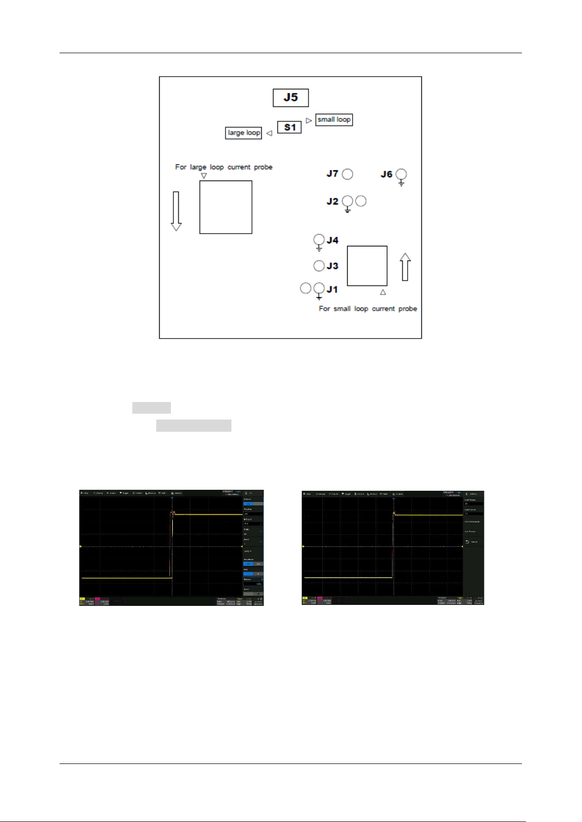
SDS6000L User Manual
int. s i g l e n t . c o m 2 3 7
C. Connect the voltage and current probes to the oscilloscope input channel
D. Click Signal to enter the signal setting menu. Select the corresponding input channel, and
then click Auto Deskew to perform the calibration. When the process completes, a
message will pop up indicating whether the deskew operation was successful or not.
Before deskew calibration
After deskew calibration
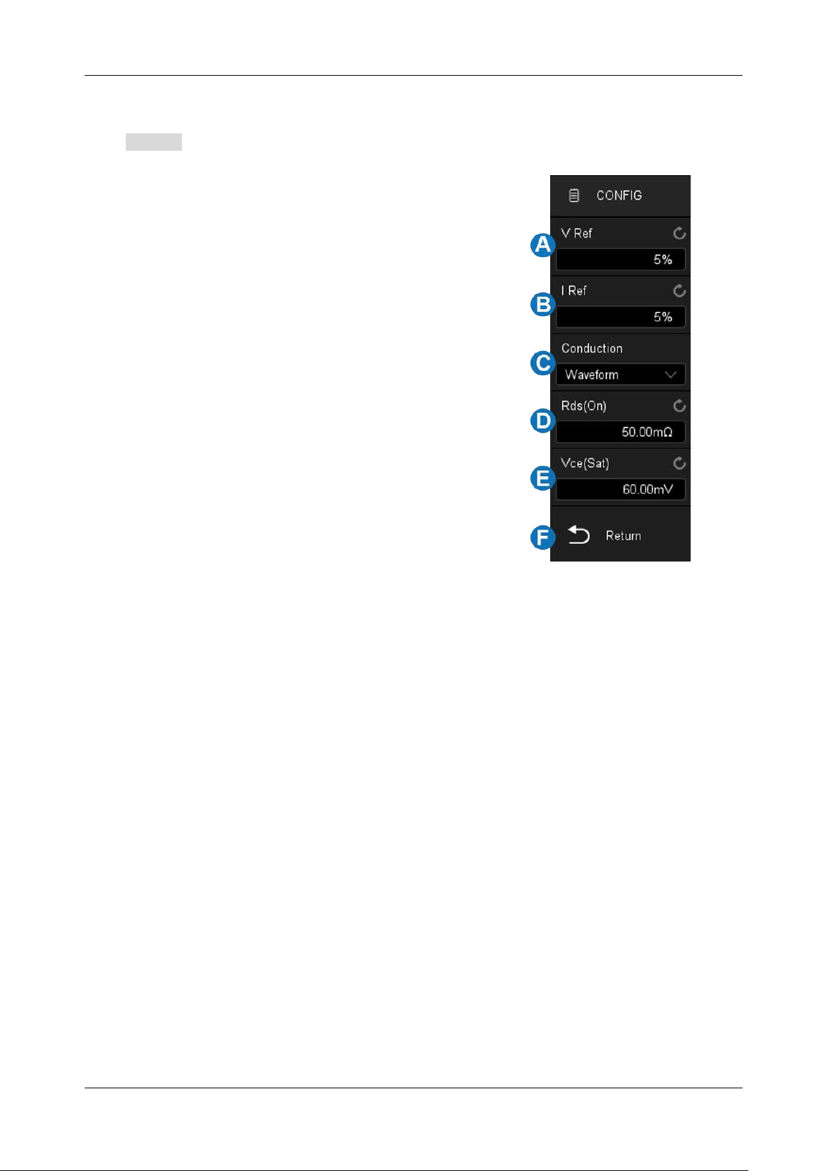
SDS6000L User Manual
2 3 8 i n t . s i g l e n t . c o m
Configuration
Click Config to recall the configuration dialog box:
A. Set the voltage reference, i.e. the switch level at the
edge of the input switch. This value is a percentage of
the maximum switching voltage. Adjusting the value
to ignore background noise. This value is used to
determine the threshold hysteresis of the switch edge
B. Set the current reference, i.e. the switch level at the
beginning of the input switch edge. This value is the
percentage of the maximum switching current. This
value can be adjusted to ignore background noise or
invalid offset that is difficult to eliminate in the current
probe. This value is used to determine the threshold
hysteresis of the switch edge
C. Set the conduction type (Waveform, Rds(on) or
Vce(sat))
D. Set Rds(on) resistance
E. Set Vce voltage
F. Return to the previous menu
Conduction Type
Waveform
-- The power waveform uses the original data, and the calculation formula is P = V * I, E =
P * T.
Rds (on)
-- In the on area (where the voltage level is lower than the voltage reference (adjustable)),
the power calculation formula is P = I
2
* Rds (on). In the off area (where the current level is lower than
the current reference (adjustable)), the power calculation formula is P = 0 watt.
Vce (sat)
-- In the on area (where the voltage level is lower than the voltage reference (adjustable)),
the power calculation formula is P = Vce (sat) * I. In the off area (where the current level is lower than
the current reference (adjustable)), the power calculation formula is P = 0 watt.
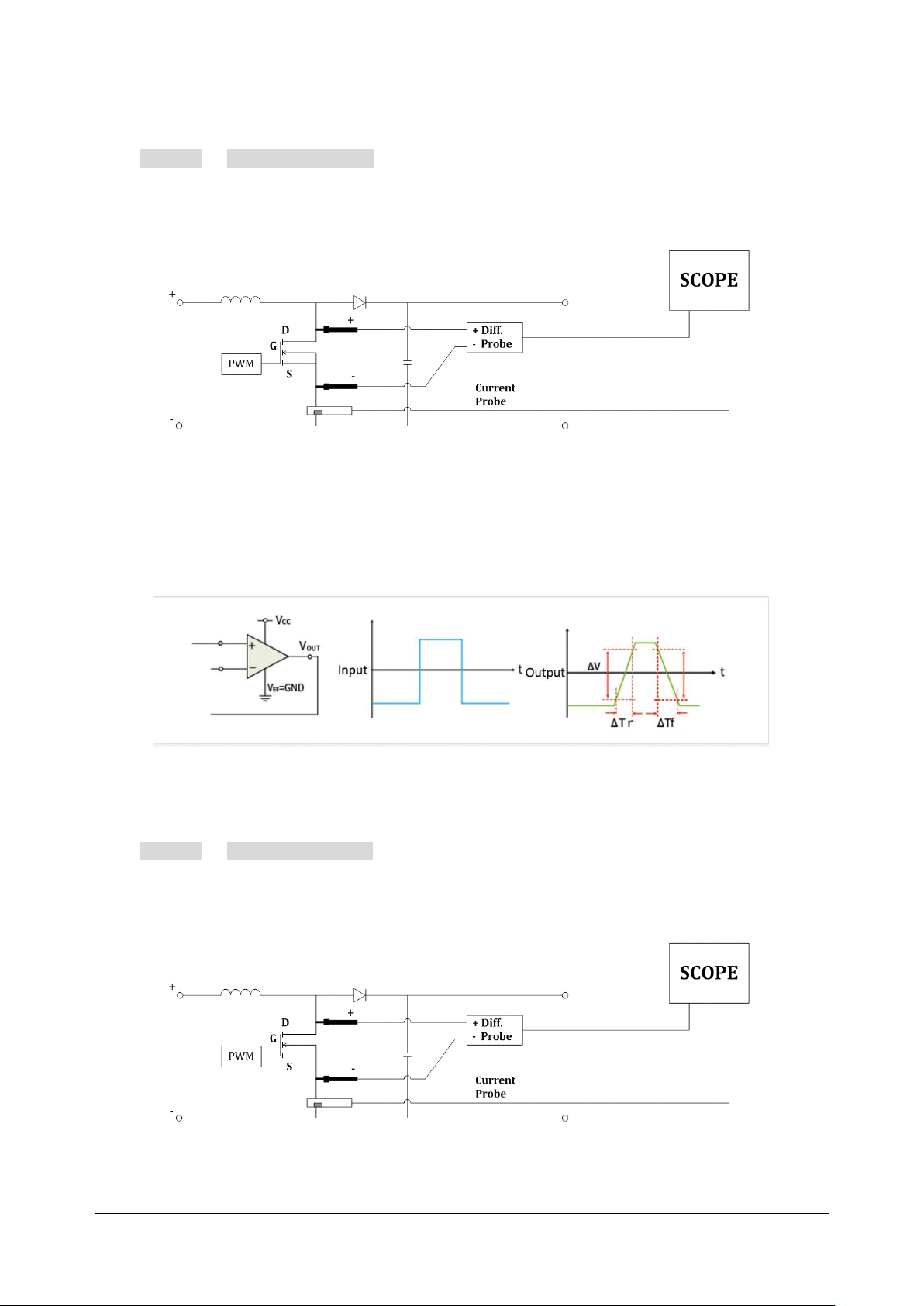
SDS6000L User Manual
int. s i g l e n t . c o m 2 3 9
Connection Guide
Click Signal > Connection Guide to recall the connection guide of switching loss, as shown in
the figure below. Please follow the instructions in this figure for connection. Click the icon on the top
right of the guide to close.
26.6 Slew Rate
The slew rate measures the change rate of voltage or current during switching.
Connection Guide
Click Signal > Connection Guide to recall the connection guide of the slew rate, as shown in the
figure below. Please follow the instructions in this figure for connection. Click the icon on the top right
of the guide to close.
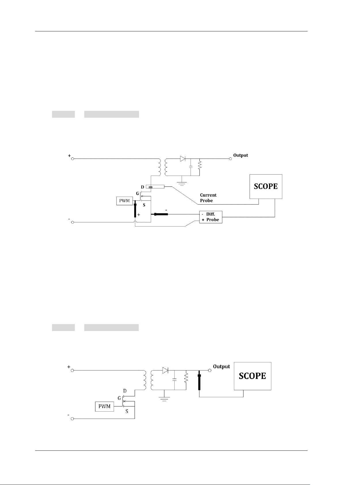
SDS6000L User Manual
2 4 0 i n t . s i g l e n t . c o m
26.7 Modulation
Modulation analysis measures the control pulse signal of the switching device (MOSFET) and observes
the pulse width, duty, period, frequency, and other trends of the control pulse signal in response to
different events.
Connection Guide
Click Signal > Connection Guide to recall the connection guide of modulation, as shown in the
figure below. Please follow the instructions in this figure for connection. Click the icon on the top right
of the guide to close.
26.8 Output Ripple
Power supply ripple is an important parameter to evaluate DC power supply, which represents the
quality of output DC voltage. Ripple analysis can measure the current value, average value, minimum
value, maximum value, standard deviation, and count of the power supply output ripple.
Connection Guide
Click Signal > Connection Guide to recall the connection guide of output ripple, as shown in the
figure below. Please follow the instructions in this figure for connection. Click the icon on the top right
of the guide to close.
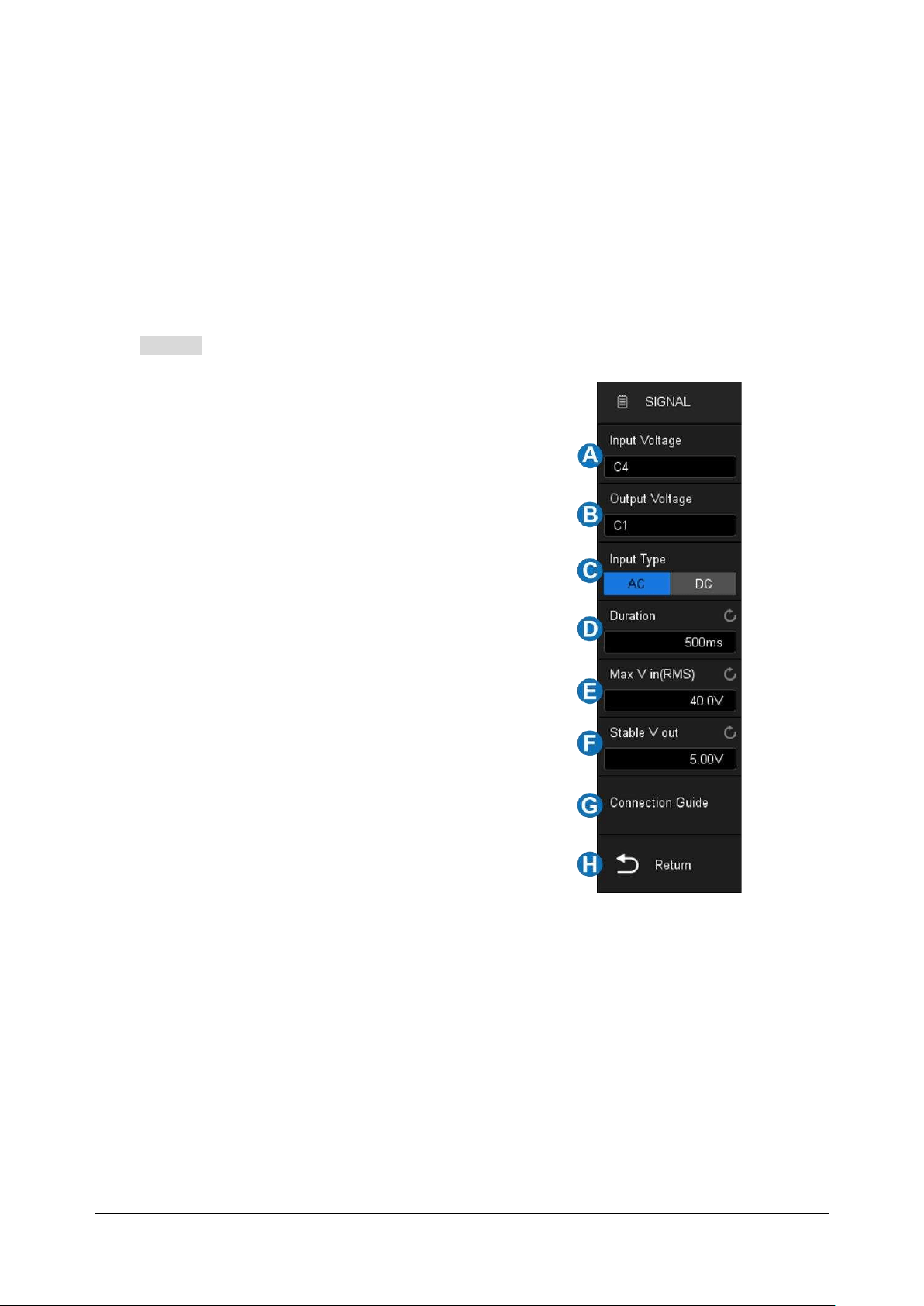
SDS6000L User Manual
int. s i g l e n t . c o m 2 4 1
26.9 Turn On/Turn Off
Turn-on analysis determines the time taken for the power supply to reach 90% of its steady-state output.
Turn-off analysis determines the time taken for the power supply to fall to 10% of its maximum output
voltage.
Signal Settings
Click Signal to recall signal settings dialog box:
A. Set the input voltage source
B. Set the output voltage source
C. Set the input type (AC or DC)
D. Set the duration, the range is 5 ns ~ 20 s. The
oscilloscope will set the timebase according to
the value (duration / 10)
E. Set the maximum effective input voltage Vrms,
the range is 1 V ~ 1 kV. The oscilloscope will
set the vertical scale of the voltage channel to
maximum input voltage / 7 and the trigger level
to maximum input voltage / 10.
F. Set the stable output voltage value, the range is
-30 V ~ 30 V. The oscilloscope will set the
vertical scale of the output voltage channel to
stable output voltage / 6
G. View the connection guide
H. Return to the previous menu
Testing Conditions
Turn On
-- Determines the time taken for the power to reach a certain percentage of its steady-state
output. The turn on time is between T2 and T1, where:
T1 = When the input voltage first rises to a certain percentage (usually 10%) of its maximum amplitude
T2 = When the output DC voltage rises to a certain percentage (usually 90%) of its maximum amplitude
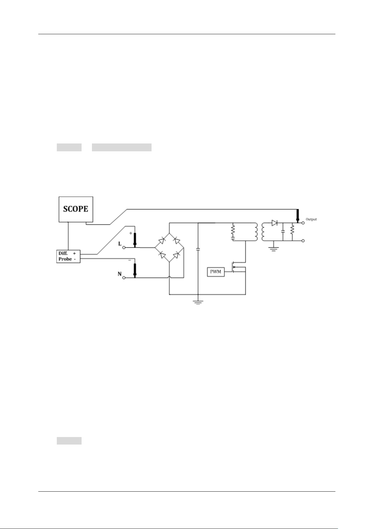
SDS6000L User Manual
2 4 2 i n t . s i g l e n t . c o m
Turn Off
-- Determines the time it has taken for the power supply to be turned off to fall to a certain
percentage of its maximum output voltage. The turn off time is between T2 and T1, where:
T1 = When the input voltage finally falls to a certain percentage (usually 10%) of its maximum amplitude
T2 = When the output DC voltage finally falls to a certain percentage (usually 10%) of its maximum
amplitude
Connection Guide
Click Signal > Connection Guide to recall the connection guide of turn on/turn off, as shown in
the figure below. Please follow the instructions in this figure for connection. Click the icon on the top
right of the guide to close.
26.10 Transient Response
Transient response analysis can determine the response speed of the output voltage of the power
supply to the change of the output load. This time starts from the first time that the output voltage exits
the stable band and ends at the last time that the output voltage enters the stable band.
Signal Settings
Click Signal to recall signal settings dialog box:
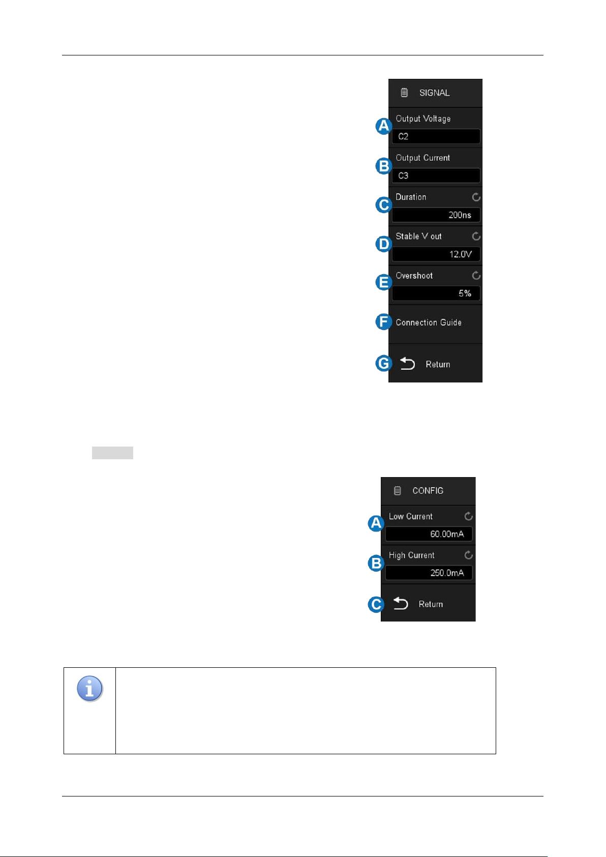
SDS6000L User Manual
int. s i g l e n t . c o m 2 4 3
A. Set the output voltage source
B. Set the output current source
C. Set the duration. The oscilloscope will set the
appropriate time base according to the
duration
D. Set the stable output voltage, i.e. the expected
output DC voltage of the power supply in a
stable state
E. Set the overshoot percentage of output
voltage, which can be used to determine the
stable band value of transient response and
adjust the vertical scale of the oscilloscope
F. View the connection guide
G. Return to the previous menu
Configuration
Click Config to recall the configuration dialog box:
A. Set the input low current value. This is the
expected low current value before or after
the load change
B. Set the input high current value. This is the
expected high current value before or after
the load change
C. Return to the previous menu
Note:
The low and high current values are used to calculate the trigger level
and adjust the oscilloscope vertical scale. After the load changes, the current
value changes from low to high (or from high to low), and the oscilloscope
triggers and performs to measure the transient response stability time.
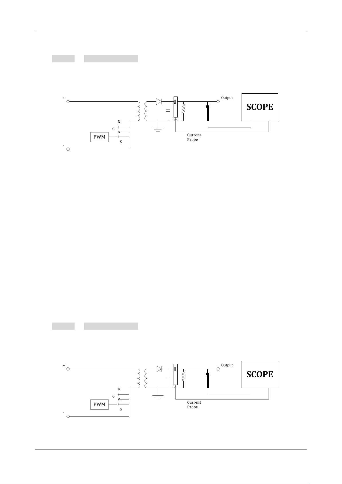
SDS6000L User Manual
2 4 4 i n t . s i g l e n t . c o m
Connection Guide
Click Signal > Connection Guide to recall the connection guide of transient response, as shown
in the figure below. Please follow the instructions in this figure for connection. Click the icon on the top
right of the guide to close.
26.11 PSRR
The power supply rejection ratio (PSRR) test is used to determine how the regulator suppresses ripple
noise in different frequency ranges. The oscilloscope controls the arbitrary waveform/function
generator to output a sweep signal, which is used to introduce ripple into the DC voltage transmitted
to the voltage regulator. Measure the AC RMS ratio of input to output, and plot the relationship between
the ratio and frequency. The background noise of the oscilloscope is higher than that of the network
analyzer, and the sensitivity is lower than that of the network analyzer, so the PSRR measured by the
oscilloscope is difficult to exceed -60 dB. The PSRR test is generally acceptable for sampling the
overall PSRR behavior of the power supply under test.
The configuration of PSRR is the same as that of the Bode plot, see the chapter "Bode Plot" for details.
Connection Guide
Click Signal > Connection Guide to recall the connection guide of PSRR, as shown in the figure
below. Please follow the instructions in this figure for connection. Click the icon on the top right of the
guide to close.
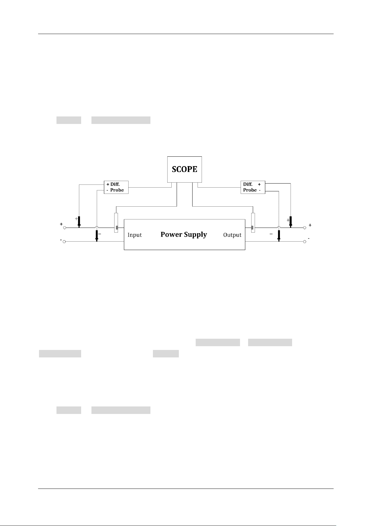
SDS6000L User Manual
int. s i g l e n t . c o m 2 4 5
26.12 Power Efficiency
Power efficiency analysis can test the overall efficiency of the power supply by measuring the output
power and input power.
Connection Guide
Click Signal > Connection Guide to recall the connection guide of power efficiency, as shown in
the figure below. Please follow the instructions in this figure for connection. Click the icon on the top
right of the guide to close.
26.13 SOA
The safe operating area (SOA) of MOSFETs defines the voltage, current, and power consumption
conditions over which the device can be expected to operate without self-damage. The oscilloscope
can automatically generate the SOA according to the Voltage Limit , Current Limit , and
Power Limit parameters set in the Config menu, and judge if the stress on the MOSFET is
beyond the SOA or not. This helps designers quickly find a problem or latent risk in the circuit.
Connection Guide
Click Signal > Connection Guide to recall the connection guide of power efficiency, as shown in
the figure below. Please follow the instructions in this figure for connection. Click the icon on the top
right of the guide to close.
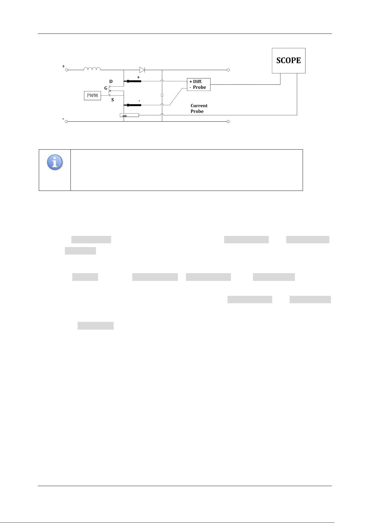
SDS6000L User Manual
2 4 6 i n t . s i g l e n t . c o m
Note:
Perform a Deskew operation between the voltage and current input
channels before the test. See the section “Switching Loss” for more details
on deskewing.
The test steps are as followed:
1. In the Input Setup menu, assign the correct channels to Input Voltage and Input Current .
Set Duration as the expected observed duration, then the oscilloscope will automatically set
the timebase according to it.
2. In the Config menu set Voltage Limit , Current Limit , and Power Limit parameters
according to the datasheet of the MOSFET device under test, then the oscilloscope will
automatically generate the SOA and the vertical scale of the Input Voltage and Input Current
channels according to them.
3. Turn on Test State . The oscilloscope will begin to acquire the voltage and current waveforms,
and display the SOA measurement, showing if the measured stresses are in the SOA or not.
4. Users can adjust horizontal, vertical, and trigger settings during the test for the best observation.
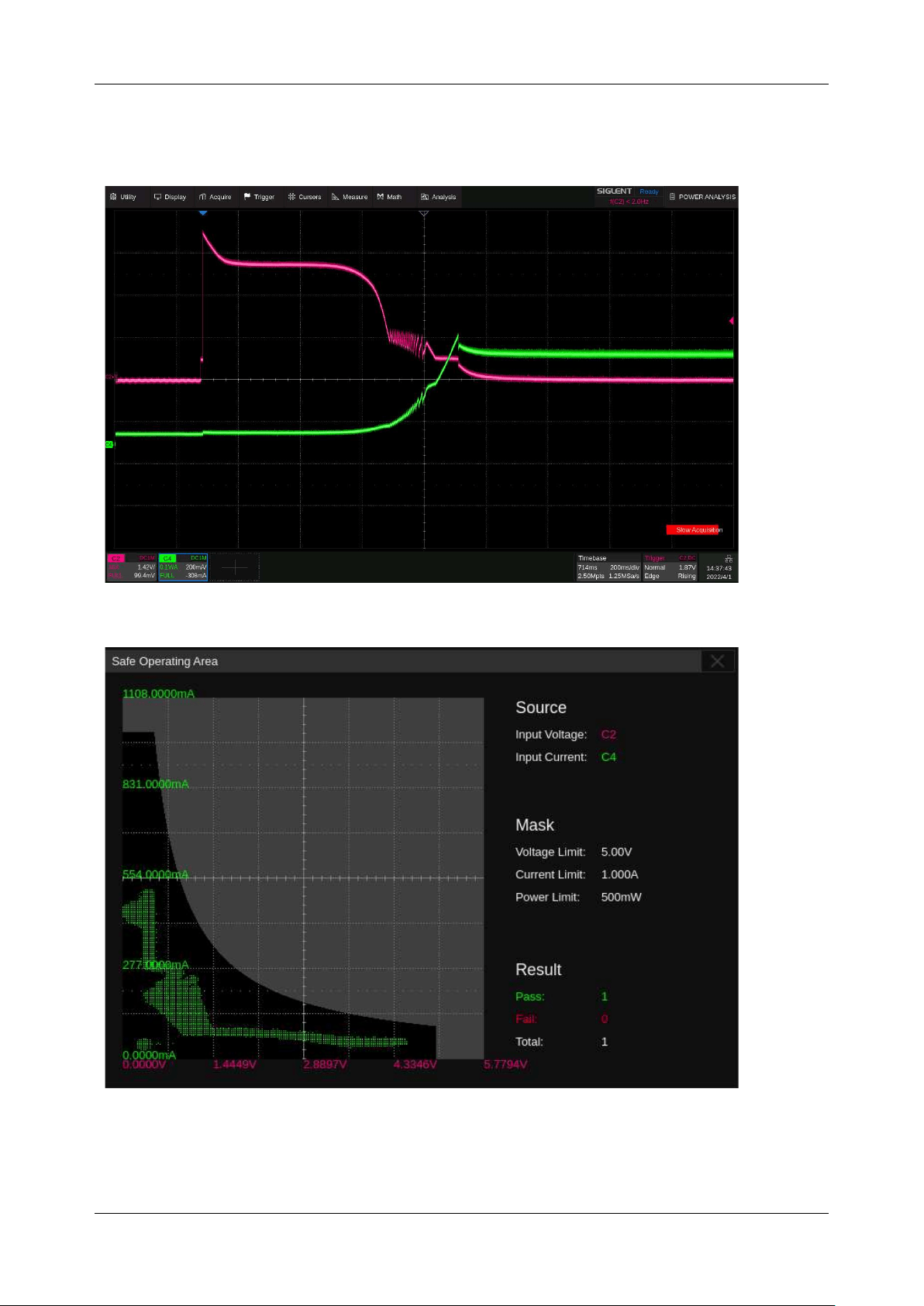
SDS6000L User Manual
int. s i g l e n t . c o m 2 4 7
Below is an example of testing the power-up stresses on a MOSFET and judging if the stresses are
safe for the MOSFET using the SOA:
Voltage and current waveforms on the MOSFET at power-up
SOA, in which the mask is created according to the voltage limit, current limit, and power
limit. The result shows “Pass” because all the stresses are within the mask.
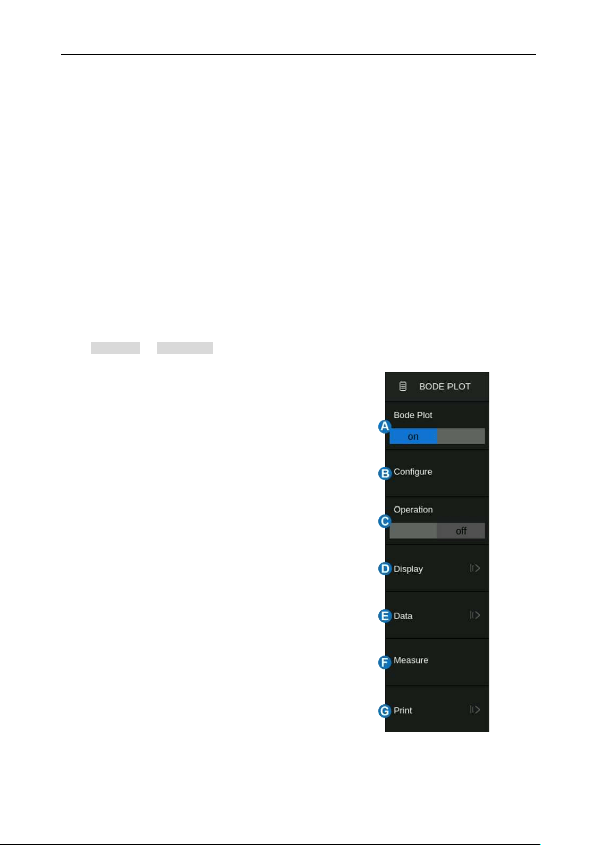
SDS6000L User Manual
2 4 8 i n t . s i g l e n t . c o m
27 Bode Plot
27.1 Overview
The SDS6000L supports an automatic Bode plot function. This function provides a frequency response
curve of the device-under-test as well as the interface for output sweep parameter control and data
display settings. At this time, either the built-in waveform generator or one of the SIGLENT SDG series
arbitrary function generators are supported. During the sweep, the oscilloscope configures the
generator output frequency and amplitude and then compares the input signal to the output of the DUT.
Gain (G) and phase (P) are measured at each frequency and plotted on the frequency response Bode
plot. When the loop response analysis is complete, you can move the markers on the chart to see the
gain and phase values measured at each frequency point. You can also adjust the scale and offset
settings for the amplitude and phase plots.
Click Analysis > Bode Plot to recall the Bode plot dialog box:
A. Turn on/off the Bode plot
B. Configure the Bode plot (DUT, AWG connection,
sweep parameters)
C. Turn on/off the operation
D. Set display parameters, including coordinate axis,
trace visibility, and cursors
E. Data list. Open the data list of the Bode plot to
view the curve data, save the data results to a
U-disk or recall it from a U-disk
F. Set the measurement parameters. Parameter
measurement of the scanning curve includes
upper cut-off frequency (UF), lower cut-off
frequency (LF), bandwidth (BW), gain margin
(GM), and phase margin (PM)
G. Quickly print the specified Bode Plot waveform
area to the storage.
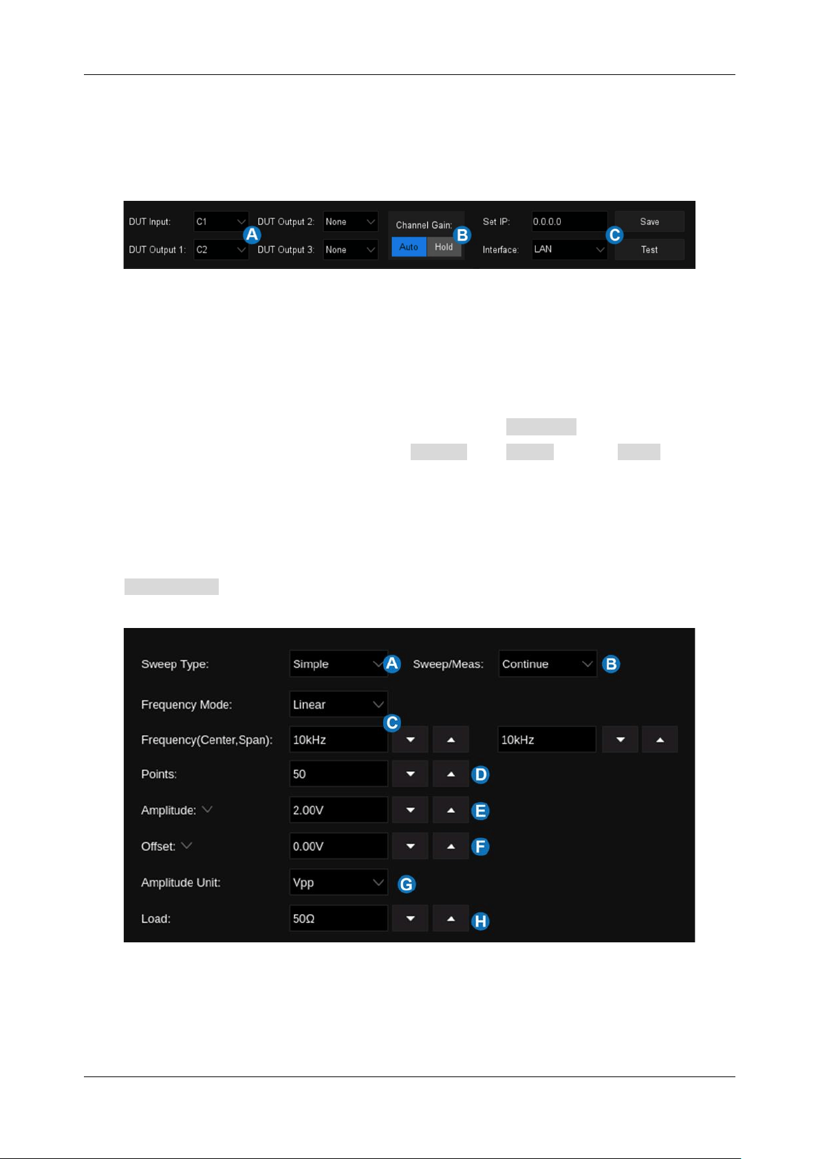
SDS6000L User Manual
int. s i g l e n t . c o m 2 4 9
27.2 Configuration
27.2.1 Connection
A. DUT input and output channels
B. Channel gain. When it is set to Auto, the oscilloscope will automatically adapt the vertical
scale according to the signal amplitude; when it is set to Hold, it will always keep the vertical
scale before the test operation
C. Arbitrary waveform generator connection settings. Click Interface to select the connection
type. When selecting LAN, it needs to Set IP and Save it. Click Test to confirm
whether the arbitrary waveform generator is connected correctly.
27.2.2 Sweep
Click Sweep Type to select the sweep type. There are two types: Simple and Variable level.
A. Set the sweep type
B. Set the sweep as Continue or Single
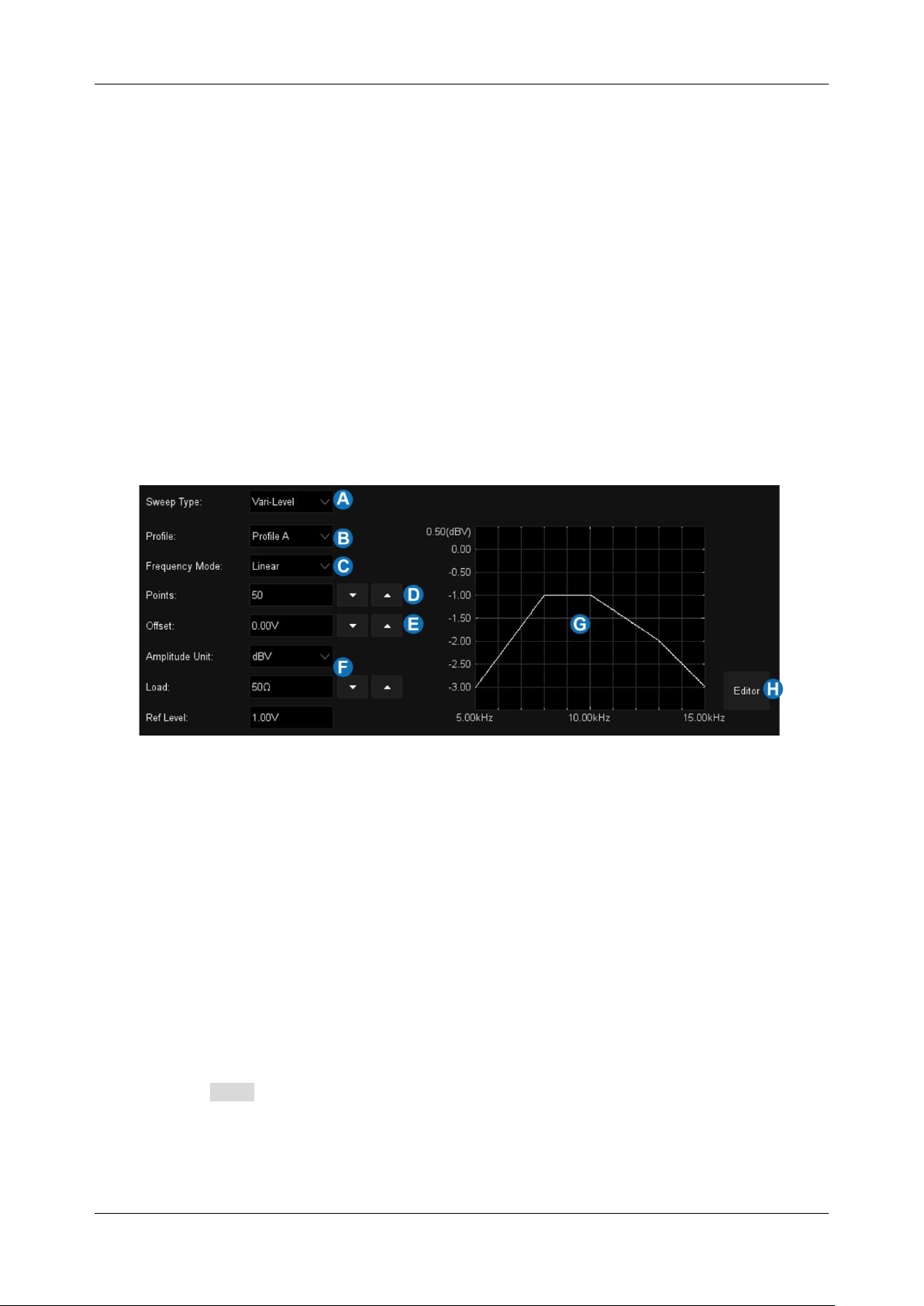
SDS6000L User Manual
2 5 0 i n t . s i g l e n t . c o m
C. Set the sweep frequency. The frequency mode can be linear or decade. When it is set to
linear, the corresponding center frequency and span frequency need to be set; when it is set
to a decade, the corresponding start frequency and stop frequency need to be set
D. Set the number of sweep points. The larger the number of points, the higher the sweep
resolution
E. Set the amplitude of the sweep signal
F. Set the offset of the sweep signal
G. Set the signal amplitude unit. When it is set to dB, the reference level and load need to be
set
H. Set the load
A. Set the sweep type to Vari-Level
B. Select a profile. Up to 4 profiles can be edited
C. Set the frequency mode
D. Set the number of sweep points
E. Set the offset of the sweep signal
F. Set the signal amplitude unit. When it is set to dB, the reference level and load need to be
set
G. Variable level signal display area
H. Click Edit to turn on the profile editor
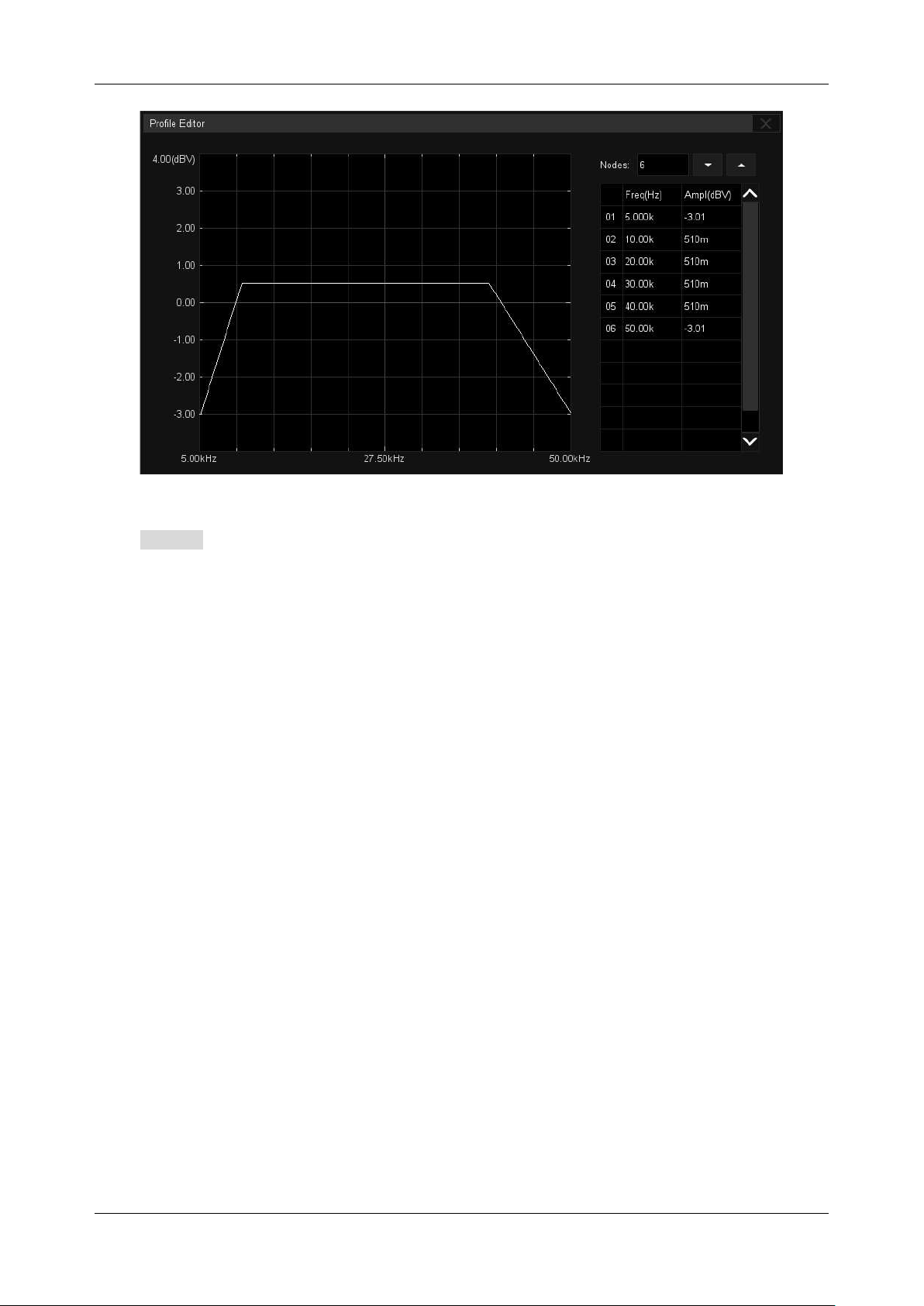
SDS6000L User Manual
int. s i g l e n t . c o m 2 5 1
Click Nodes to set the signal node number through the mouse wheel, or click ▲ to increase the
nodes and ▼ to decrease.
Click the cell in the table area to set the frequency and amplitude of the corresponding node. Click to
activate the cell, adjust the value through the mouse wheel, or click the cell again to call up the virtual
keypad for setting.
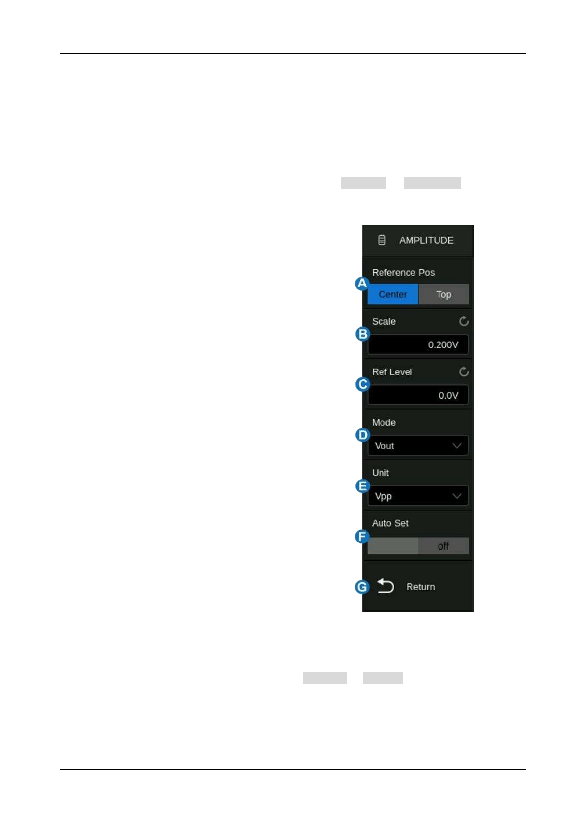
SDS6000L User Manual
2 5 2 i n t . s i g l e n t . c o m
27.3 Display
Bode plot display settings include amplitude, phase, cursors, and trace visibility.
Amplitude
Set the amplitude coordinate axis of the Bode plot. Click Display > Amplitude to recall the
amplitude setting dialog box:
A. Set the reference position to the center or top
B. Set the scale of the amplitude coordinate axis
C. Set the reference level, the max value of the
amplitude coordinate axis
D. Set the amplitude mode. Set to Vout to display
the amplitude value of the output signal; set to
Vout/Vin to display the amplitude ratio of the
output signal to the input signal
E. When the mode is Vout, it needs to set the
unit (Vpp, Vrms, dBV, dBu, dBm, or Arbitrary
dB); when the mode is Vout/Vin, it needs to
set the amplitude axis type (Linear or
Logarithmic).
F. Auto-Set. According to the output signal
amplitude curve, the oscilloscope
automatically sets the scale and reference
level
G. Return to the previous menu
Phase
Set the phase coordinate axis of the Bode plot. Click Display > Phase to recall the phase setting
dialog box:
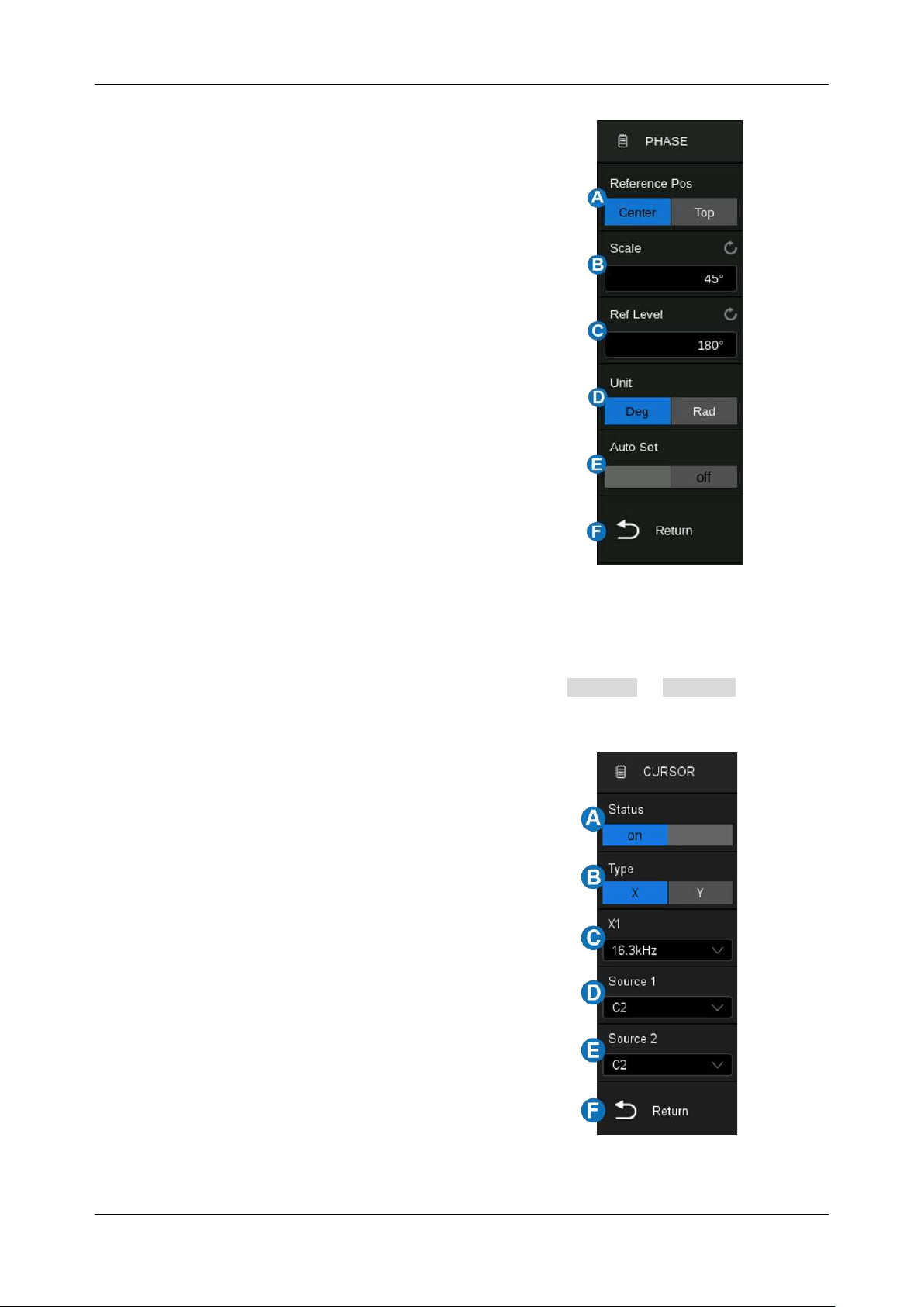
SDS6000L User Manual
int. s i g l e n t . c o m 2 5 3
A. Set the reference position to the center or top
B. Set the scale of the phase coordinate axis
C. Set the reference level, the max value of the
phase coordinate axis
D. Set the phase unit (Degree or Rad)
E. Auto-Set. According to the output signal phase
curve, the oscilloscope automatically sets the
scale and reference level
F. Return to the previous menu
Cursors
SDS6000L can use the cursor to measure the Bode plot curve. The cursor of the Bode plot is similar
to the ordinary cursor, see the chapter "Cursors" for details. Click Display > Cursors to recall the
cursor setting dialog box.
A. Turn on/off the cursors of the Bode plot
B. Set the cursors type (X or Y)
C. Specify the cursor and set the position
D. Set the source 1
E. Set the source 2
F. Return to the previous menu
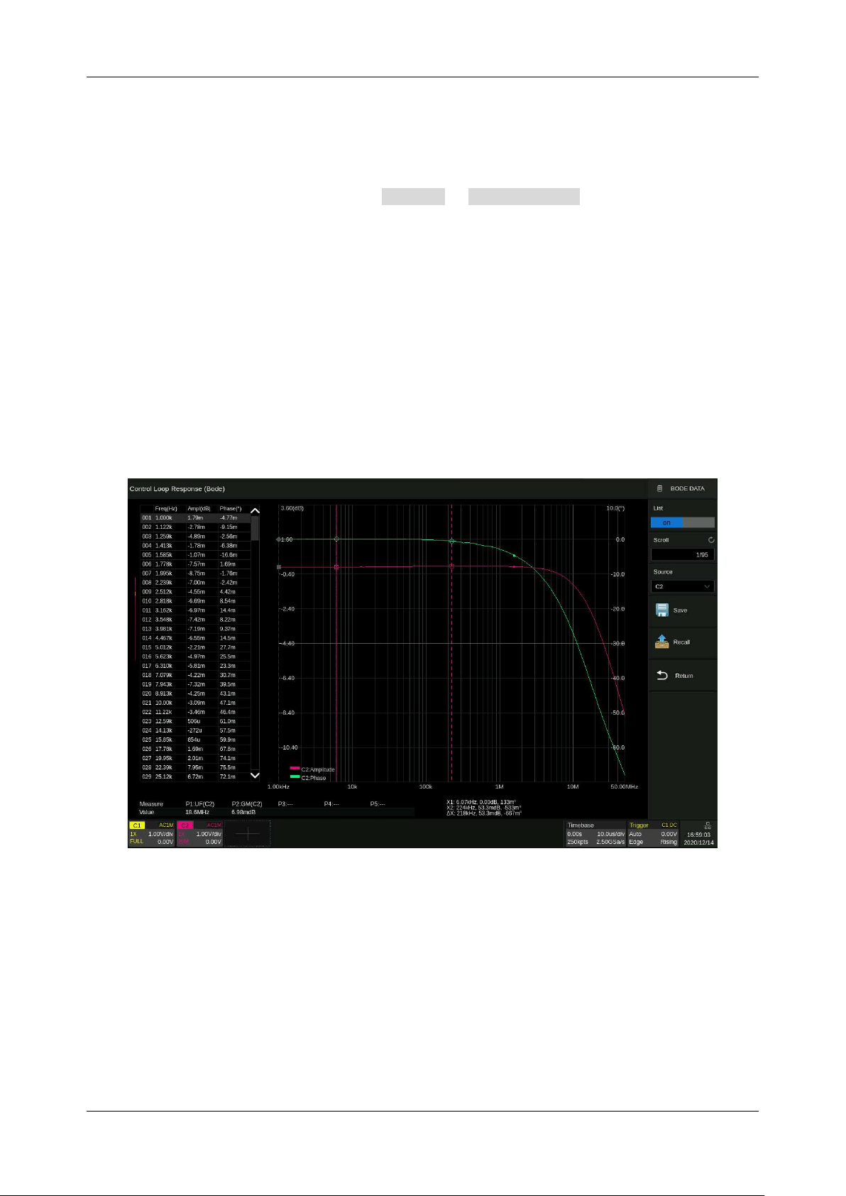
SDS6000L User Manual
2 5 4 i n t . s i g l e n t . c o m
Trace Visibility
When multiple output signals are connected, the Bode plot interface will display the amplitude and
phase curves of all output signals at the same time. Users can turn on/off other scanning curves to
observe the details of specific curves. Click Display > Trace Visibility to recall the setting dialog
box.
27.4 Data Analysis
With the data list, cursor measurement, and automatic measurement functions, the Bode plot curve
can be analyzed in detail. The data list provides the raw values for each point. The cursors can be
used to flexibly measure the change of each position of the curve. The automatic measurement function
can be used to measure the five parameters of the Bode plot curve: upper cut-off frequency (UF), lower
cut-off frequency (LF), bandwidth (BW), gain margin (GM), and phase margin (PM).
A. Data list display area
B. Cursors
C. Data point location line
D. Cursor information display area
E. Measurement parameters display area
F. Bode plot dialog box
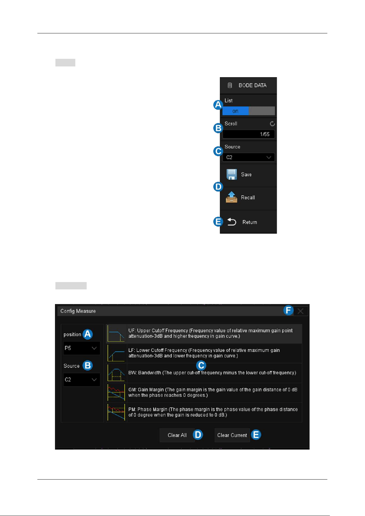
SDS6000L User Manual
int. s i g l e n t . c o m 2 5 5
Data List
Click Data to recall the data setting dialog box:
A. Turn on/off the data list
B. Set the selected row in the list. Adjust
the mouse wheel to set, or directly
click the list display area to select a
specific line.
C. Set the data source
D. Save/Recall the data. Saving and
recalling the Bode plot data (*.csv) is
similar to the operation of setup files,
see the chapter "Save/Recall" for
details
E. Return to the previous menu
Measure
Click Measure to recall the measure setting dialog box:

SDS6000L User Manual
2 5 6 i n t . s i g l e n t . c o m
A. Set the position of measurement items, and support 5 measurement items at most
B. Set the measurement source
C. Measurement parameter area. Click each parameter area to activate the measurement
parameter. In the figure above, "UF" is activated.
D. Clear all measurements
E. Clear the current measurement
F. Close the measurement configuration window
For example, to add UF measurements for C2 and GM measurements for C3, follow the steps below:
Measure > Position > Source > UF
Measure > Position > Source > GM
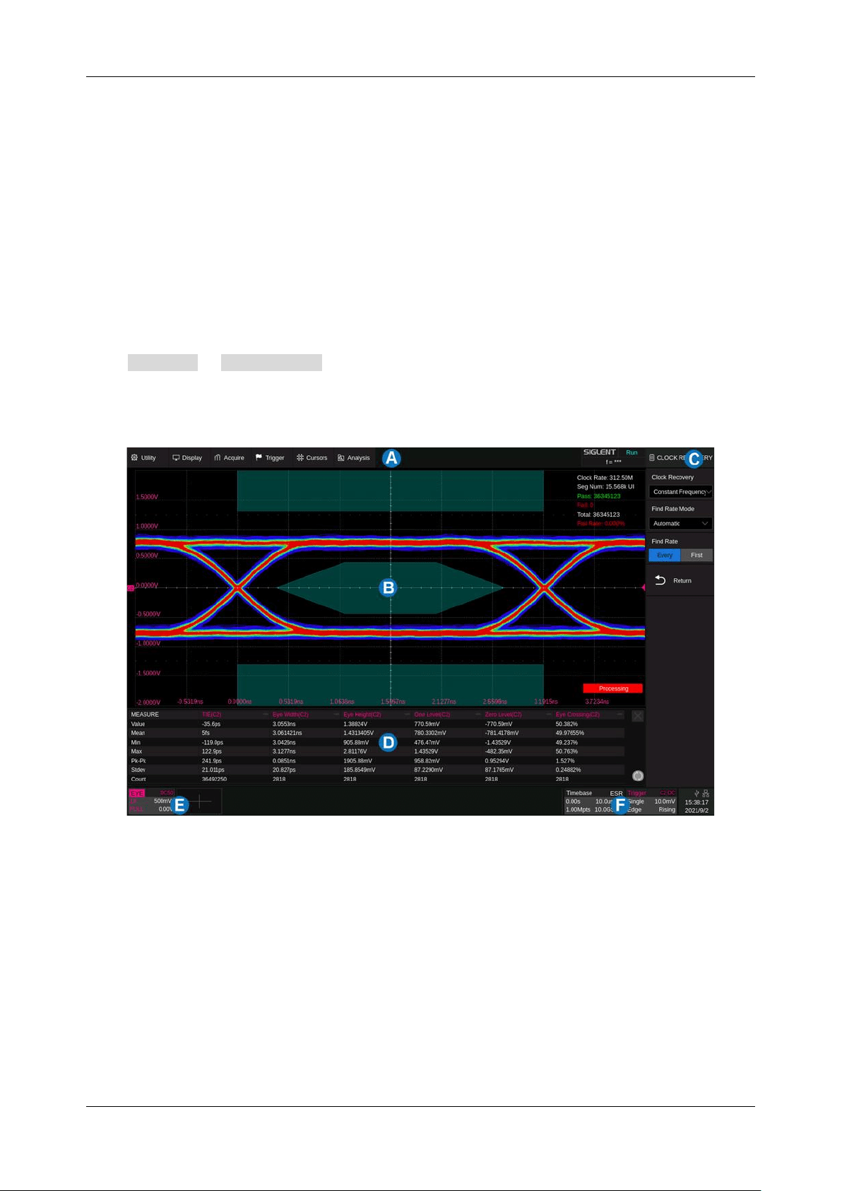
SDS6000L User Manual
int. s i g l e n t . c o m 2 5 7
28 Eye Diagram
28.1 Overview
An eye diagram is an oscilloscope display in which a high-speed digital signal is repetitively sampled
and applied to the vertical input, while the data rate is used to trigger the horizontal sweep. It is called
an Eye because the pattern looks like a series of eyes between a pair of rails. The combined effects of
channel and dispersion can be evaluated from the Eye opening width and height.
Click Analysis > Eye Diagram to recall the diagram analysis dialog box, this process may take
several seconds. The user interface is similar to normal mode.
A. Menu Bar
B. Grid Area
C. Dialog Box
D. Measurement parameters display area
E. Eye diagram descriptor box, click to recall the eye diagram dialog box
F. Timebase and Trigger descriptor box
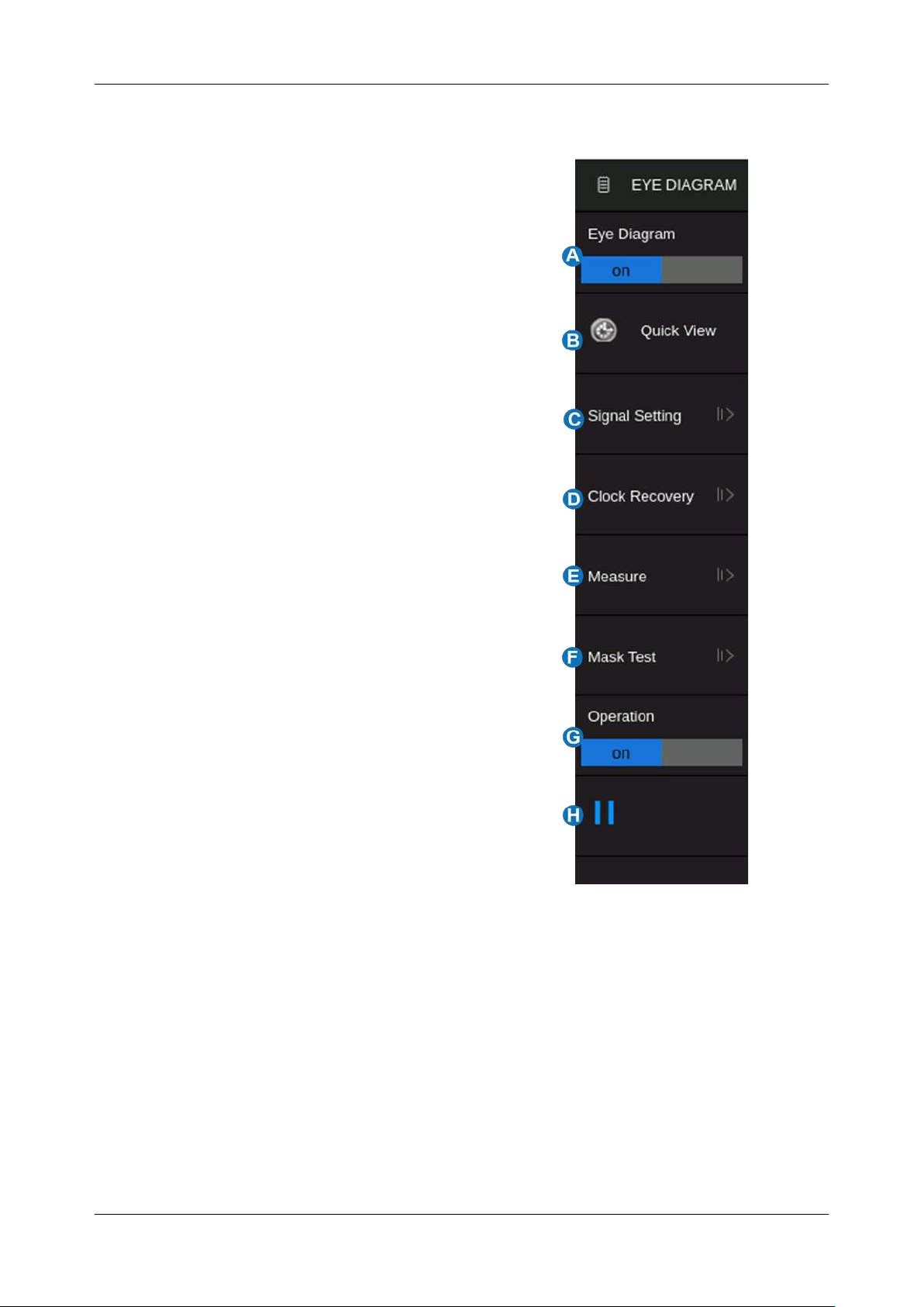
SDS6000L User Manual
2 5 8 i n t . s i g l e n t . c o m
Eye Diagram Dialog Box:
A. Turn on/off the eye diagram
B. Quick view. The oscilloscope will automatically
adjust its vertical/horizontal scale and trigger
level after the corresponding channel source is
set and the quick view option is active
C. The signal setting, including source selection
and level adjustment
D. Clock recovery options, including Constant
Frequency and PLL
E. Measure, similar to Measure in normal mode
F. Mask test
G. Turn on / off the operation. It is allowed to
enter the Y-T mode without exiting the eye
diagram if run off the operation.
H. Run / Stop eye diagram when the operation is
active.
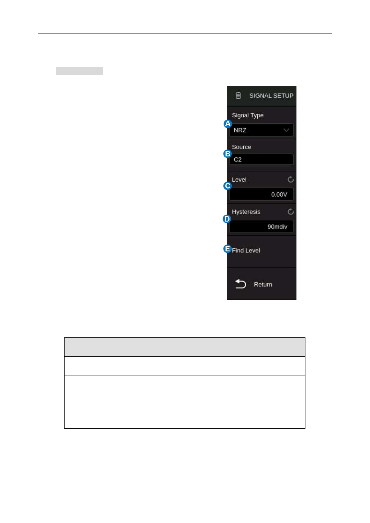
SDS6000L User Manual
int. s i g l e n t . c o m 2 5 9
28.2 Signal Setting
Click Signal Setting to open the signal setup dialog box.
A. Signal Type: NRZ, 100Base-TX
B. The source can be C1~C8.
C. Set the trigger level manually
D. The hysteresis of the trigger level has a unit
of division in the vertical direction. A Larger
hysteresis range comes with better noise
tolerance but reduced sensitivity. A larger
hysteresis range requires a higher signal
amplitude.
E. The find level indicates that the oscilloscope
will automatically seek and set the trigger
level at the intersection of the rising and
falling edges of the eye diagram.
Table 28.1 Description of Signal Type
Signal Type
Description
NRZ
General NRZ (non-return-to-zero) code
100Base-TX
MLT-3 (Multi-Level Transmit) code that uses three voltage
levels. When Signal Type = 100Base-TX, there are two
available levels (upper level for the upper eyes, and lower
level for the lower eyes);
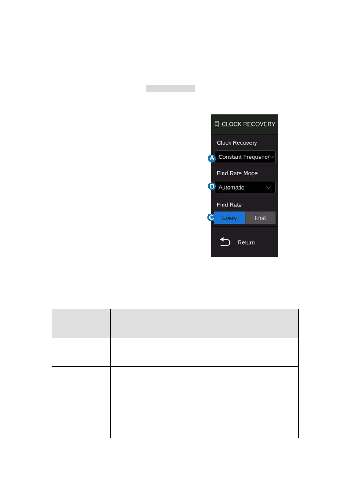
SDS6000L User Manual
2 6 0 i n t . s i g l e n t . c o m
28.3 Clock Recovery
Clock recovery is a feature that provides an ideal clock for comparison to actual signal edges. It is the
key step in constructing an eye. The eye diagram can be constructed only when the reference clock is
recovered from the data correctly. Click Clock Recovery in the eye diagram menu to open the dialog
box.
A. Set the clock recovery method, Constant
Frequency, or PLL. See Table 28.2 for
details.
B. Choose the mode of finding rate between
Manual and Automatic.
C. Choose the find rate between Every and
First. The oscilloscope will perform a
clock recovery for each acquisition in the
“Every” mode and at each new frame, the
eye diagram will replace the clock rate
with the one from the previous frame. In
the “First” mode, the oscilloscope uses
the clock recovered from the first frame
for all the frames
Table 28.2 Description of Clock Recovery Method
Clock Recovery
Method
Description
Constant
Frequency
The clock is assumed to be a constant frequency and recovered
through the linear fitting based on the least-squares method.
Phase-Locked
Loop
The value of each reference clock edge will be calculated by the
PLL software based on the sampled signal. Using this method, the
low-frequency components in the jitter can be removed because of
the tracking capacity of the PLL. This method supports First Order
Golden PLL and its loop bandwidth can be configured by changing
the damping factor.
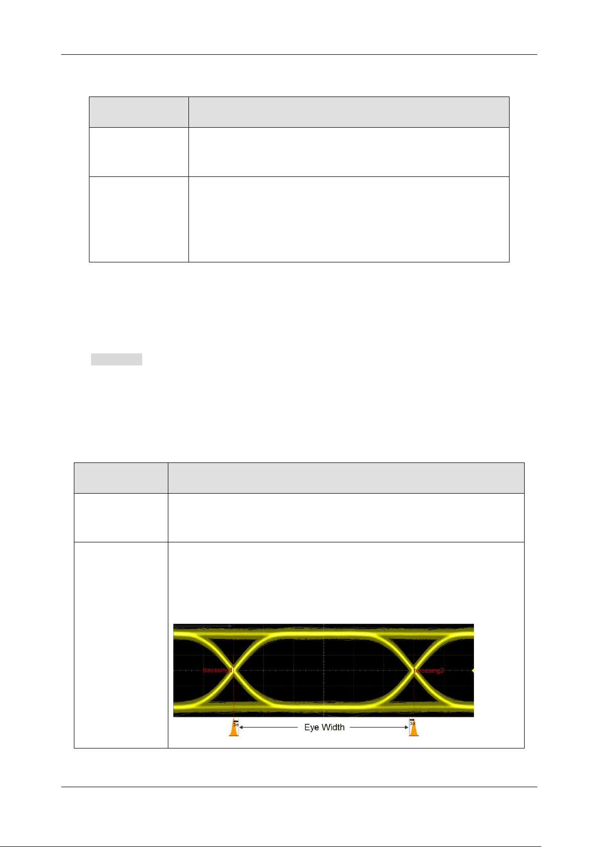
SDS6000L User Manual
int. s i g l e n t . c o m 2 6 1
Table 28.3 Description of Clock Data Rate
Date Rate
Description
Automatic
The clock is recovered using the signal edge database only. It is
the recommended method in most cases.
Manual
The oscilloscope will perform clock recovery under the expected
Data Rate as your input. Suitable for the situations in which the
oscilloscope cannot recover the clock accurately when the signal-
to-noise ratio is poor.
28.4 Measurement
Click Measure under the eye diagram menu to open the measurement setting dialog.
The measurement under the eye diagram mode is similar to measurements in normal mode. Refer to
Chapter “Measurement” to see the operating instructions.
Table 28.4 Description of Eye Diagram Parameters
Parameters
Description
Time Interval
Error
TIE is the difference between the edges in a data signal and the edges in
an ideal data signal
Eye Width
The horizontal opening of an eye diagram. Estimated based on the
distribution of the eye diagram crossing point in the horizontal direction.
( ) ( )
crossin g2 crossin g 2 crossin g1 crossin g1
EyeWidth= t -3 - t +3
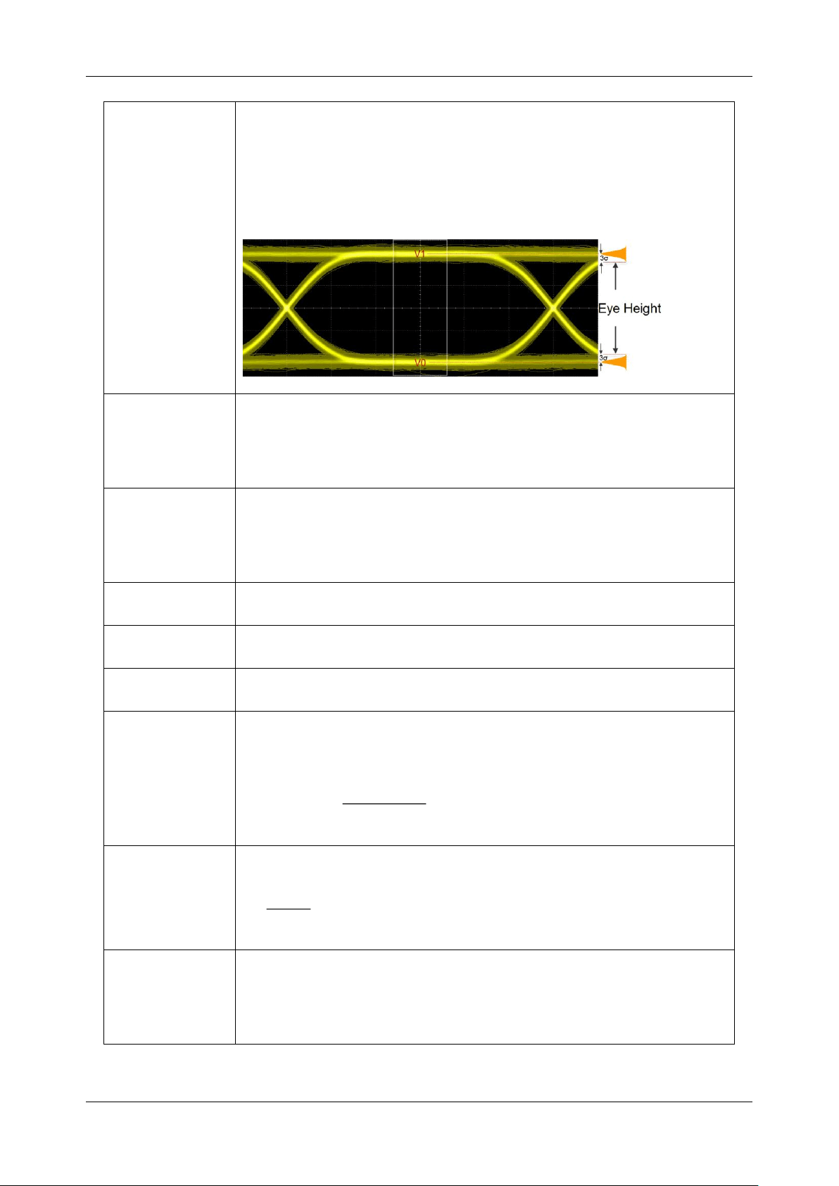
SDS6000L User Manual
2 6 2 i n t . s i g l e n t . c o m
Eye Height
The vertical opening of an eye diagram. Estimated based on the vertical
distribution of the measured high-voltage and measured low-voltage in the
40% to 60% UI interval.
( ) ( )
1 1 0 0
EyeHeight= V -3 - V +3
1-level
The high voltage corresponds to 1-level in the diagram. The one level is
calculated as the mean value of the top histogram distribution in the middle
20 percent of the eye period
0-level
The low voltage corresponds to the 0-level in the diagram. The zero level
comes from the histogram mean value of the data captured inside the
middle 20 percent of the eye period
Eye Amplitude
The eye amplitude describes the voltage between 1-level and 0-level
Rise Time
The duration of rising time from 20% to 80%
Fall Time
The duration of falling time from 80% to 20%
Eye Crossing
The measure of the amplitude of the crossing point relative to the one and
zero level
Crossin g 0
10
VV
Crossing(%)=
VV
−
−
Signal-to-Noise
Ratio
The ratio of the desired signal level to the level of background noise.
10
10
VV
Q=
−
+
Average Power
The average value of the whole data stream. A higher percentage of 1-
level comes with a higher average power. The figure comes to 50% of eye
amplitude when the 1-level and 0-level account for the same probability

SDS6000L User Manual
int. s i g l e n t . c o m 2 6 3
28.5 Mask Test
Click the Mask Test under the eye diagram menu to start the mask test configuration. Its principle
and operation process are the same as the mask test in normal mode. Refer to “Mask Test” to see the
details.
28.6 Other Operation
Some operations are supported under both the eye diagram analysis and normal mode. Part of the
compatible operations are listed in the following table. For details of their operations, please refer to
their respective sections.
Table 28.5 Operations that be supported under the eye diagram
Operation
Note
Vertical Control
The vertical scale (volts/div) and vertical position can be
adjusted.
Horizontal
Control and
Sampling
The horizontal scale (time/div) and trigger delay can be
adjusted. Memory depth will adjust according to the time
base under the highest sampling rate.
Trigger Control
The trigger setting is supported. Keeping the default edge
trigger mode and trigger level to ensure the oscilloscope can
trigger correctly will be recommended.
Display
The color temperature, waveform intensity, and grid are
supported to adjust.
Cursors
Both vertical and horizontal cursors can be added and
adjusted.
System
System-related settings, I/O settings, etc.
SDS6000L User Manual
2 6 4 i n t . s i g l e n t . c o m
29 Jitter Analysis
29.1 Overview
Jitter — The time deviation from the ideal timing of a data-bit event — is one of the most important
topics in high-speed digital data signals. The Jitter analysis application featured in this device can
measure kinds of jitter features. Besides, the various jitter components can be decomposed based on
TIE data and analyzed in time and frequency domains.
Click Analysis > Jitter to recall the jitter analysis dialog box, this process may cost several
seconds. Its user interface is similar to the UI in an eye diagram or normal mode.
A. Menu Bar
B. The grid area displays the waveform in normal or eye diagram modes.
C. Dialog Box
D. Measurement parameter display area
E. Clock or data rate information area
F. Timebase and Trigger descriptor box
SDS6000L User Manual
int. s i g l e n t . c o m 2 6 5
Jitter Analysis Dialog Box
A. Turn on/off the Jitter Analysis
B. Set the display mode, including Waveform
and Eye diagram
C. The signal setting, including source and
trigger level
D. Quick view. After setting the channel
source and performing a quick view, the
oscilloscope will automatically adjust the
vertical/horizontal scale and trigger level,
the frequently-used measurement types
will be recalled as well
E. Clock recovery options, including Constant
Frequency and PLL
F. Jitter decomposition setting
G. Set the measurement
29.2 Signal Configuration
Click Signal to set the channel source and trigger level. The setting is similar to Eye Diagram. Refer
to the “Signal Setting” section in the "Eye Diagram" chapter for details.
The type of measured signal can be pre-set to be data or clock in the jitter analysis, then the
oscilloscope will execute corresponding optimization processing for the signal type, which is different
from Eye Diagram.
SDS6000L User Manual
2 6 6 i n t . s i g l e n t . c o m
29.3 Clock Recovery
The setting of clock recovery is the same as Eye Diagram. Refer to the section "Clock Recovery" in
the "Eye Diagram" chapter.
29.4 Jitter Decomposition
Jitter typically consists of various jitter components that are caused by different jitter sources. For an
analytical approach, a jitter model is frequently used, which splits jitter into two major categories of
random and deterministic jitter.
Figure 29.1 Jitter decomposition tree
The benefits of jitter decomposition
:
1. Jitter performance plays a crucial role in the bit error rate of a high-speed digital
communication system. Through a limited sample, the jitter measurement value can be used
to estimate the TJ at any bit error rate if the RJ estimation is correct.
2. Jitter decomposition is a key tool to accurately derive each type of jitter as well as total jitter
in a system and identify the root causes of jitter quickly.
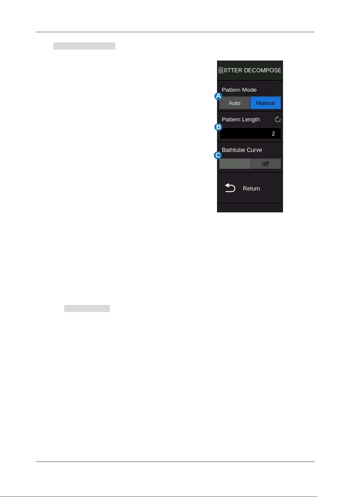
SDS6000L User Manual
int. s i g l e n t . c o m 2 6 7
Click Jitter Decomposition to enter the jitter decomposition configuration menu.
A. Set the pattern mode between Auto and
Manual. In the Manual mode, the pattern
length in bits, which represents the repetition
period of the data sequence, can be set as
user input. In the Auto mode, the pattern
length is automatically detected
B. Pattern length. When Pattern Mode = Auto,
this area is read-only. The pattern length is a
necessary parameter to calculate DCD and
DDJ
C. Enable/Disable the Bathtub plot. The "bottom"
of the bathtub expresses the degree of the
eye opening under the target bit error rate.
The result of jitter decomposition will be shown in the measured area. Users can add the jitter
components interested, including measurement values, histogram, track, and spectrogram.
29.5 Jitter Measure
Click the Jitter Measure in the Jitter analysis menu to recall the jitter measurement settings. The
operation method of adding jitter measurement parameters is the same as that of the measure closed
jitter function. Refer to the “Measurement” for details.
Statistics for each measurement item are automatically enabled when the measurement is activated.
Following are the descriptions of some jitter parameters.

SDS6000L User Manual
2 6 8 i n t . s i g l e n t . c o m
Table 29.1 Descriptions of jitter parameters
Parameter
Description
Jitter Basics
Period
The time between the crossing points of two consecutive like-polarity
edges. For clock data only.
Frequency
Reciprocal of the period. For clock data only.
+Width
Time difference between the middle of a rising edge to the middle of
the next falling edge of the pulse.
-Width
Time difference between the middle of a falling edge to the middle of
the next rising edge of the pulse.
+Duty
Positive Duty Cycle. The ratio of positive width to period. For clock
data only.
-Duty
Negative Duty Cycle. The ratio of negative width to period. For clock
data only.
CCJ
The difference between two continuous periods. For clock data only.
+Width@C2C
Difference between the positive pulse width of two continuous
cycles. For clock data only.
-Width@C2C
Difference between the negative pulse width of two continuous
cycles. For clock data only.
+Duty@C2C
Difference between the positive duty cycle of two adjacent cycles.
For clock data only.
-Duty@C2C
Difference between the negative duty cycle of two adjacent cycles.
For clock data only.
Decomposition
TIE
Time Interval Error (TIE) is the time difference between the signal
edge and the reference clock.

SDS6000L User Manual
int. s i g l e n t . c o m 2 6 9
RJ
Random jitter (RJ) also called Gaussian jitter, is unpredictable
electronic timing noise. RJ is caused by thermal noise in an electrical
circuit or due to the central limit theorem. Random jitter is unbounded
and commonly specified by the standard deviation σ. Due to its
irregular nature, random jitter (RJ) is uncorrelated to any other signal
and unpredictable in timing behavior.
DJ
Deterministic jitter, the observed peak-to-peak value will not grow
over time, has a bounded distribution.
DCD
Duty cycle distortion (DCD) is the difference between mean TIE for
rising edges and mean TIE for falling edges. Asymmetrical rise-time
vs. fall-time and non-optimal choice of decision threshold will cause
DCD.
DDJ
Data-dependent jitter (DDJ) has several discrete line distributions,
mainly caused by ISI, the physical/electrical effect. There will be
different zero-crossing positions, due to transmission line effects like
reflections and the step response of the system.
PJ
Periodic jitter (PJ) is mainly caused by periodic signal interference on
the board, including power supply ripple, clock crosstalk, etc.
Periodic interference can directly cause phase modulation of the
observed signal.
TJ@BER
Total jitter (TJ) is computed with a required bit error rate (BER) for
the system:
The value of
changes according to different bit error rates. A
common BER used in communication standards such as Ethernet is
10−12,
Part of the measurements can be displayed in frequency domains. Click the Spectrum in the dialog
of jitter measure to enter the frequency domain setting.
The vertical and horizontal parameters can be adjusted for better observation.

SDS6000L User Manual
2 7 0 i n t . s i g l e n t . c o m
29.6 Other Operation
Some operations are supported under both the jitter analysis and normal mode. The compatible
operations are similar to the eye diagram, take Table 28.5 as a reference.
29.7 System Effect on Jitter Measure
The system's influence on the jitter measurement must be taken into consideration. It is important to
evaluate the degree of error introduced in the jitter measurement according to the specifications of the
measurement system itself. The methods applied to the measuring process also play an important role
in the jitter measurement.
The system error formula of oscilloscope jitter measurement is as follows:
2
2
Sample Clock
Noise
err Jitter
Slew rate
=+
Sample clock jitter and noise in the formula are possible from the oscilloscope itself. Besides, the slew
rate of the signal under test also is related to the system error according to the formula. The slew rate
is inversely proportional to the error when the noise value does not change. This indicates that we
should use signals with edges as fast as possible during jitter testing, and keep the signal at full scale
of the oscilloscope by adjusting the vertical scale.
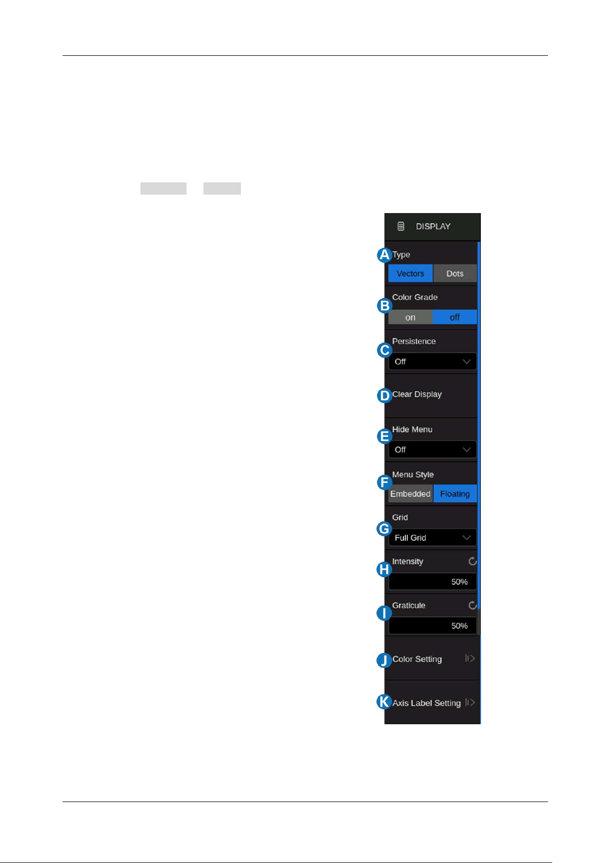
SDS6000L User Manual
int. s i g l e n t . c o m 2 7 1
30 Display
Display settings include display type of waveform, color, persistence, grid type, trace brightness,
graticule brightness, etc.
Click the menu Display > Menu to recall the display dialog box.
A. Switch the waveform display type to Vectors
(line display) or Dots
B. Turn on or off the color grade
C. Set persistence
D. Clear display. The operation clears all
waveforms displaying on the screen and
clears persist
E. Set menu auto-hide time
F. Set the menu style to Embedded or Floating.
When set to Embedded, the grid area will be
compressed horizontally to display the
complete waveform when the dialog box is
displayed. When set to Floating, it will
directly cover part of the grid area when the
dialog box is displayed
G. Select the grid type (Full Grid, Light Grid,
and No Grid)
H. Set the trace intensity (0~100%)
I. Set the graticule brightness (0~100%)
J. Customize the colors of waveforms
K. Display the axis labels
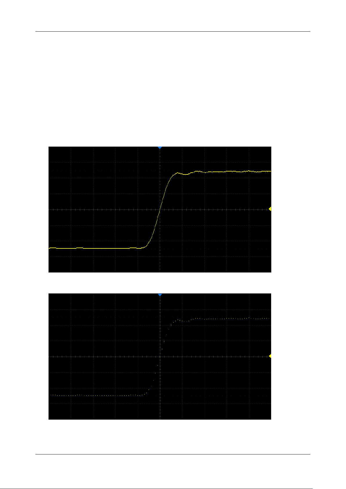
SDS6000L User Manual
2 7 2 i n t . s i g l e n t . c o m
Display Type
There is no difference between the vector and dot display types when the number of samples of a
frame is greater than 1250. When the sample number is below 1250, there are some differences.
Vectors:
The samples are connected by lines (i.e. interpolated) and displayed. The interpolation
methods include linear interpolation and sin(x)/x interpolation. See the section of "Acquisition
Setup" for details of interpolation.
Dots:
Displays the raw samples directly.
Vector Display
Dot Display
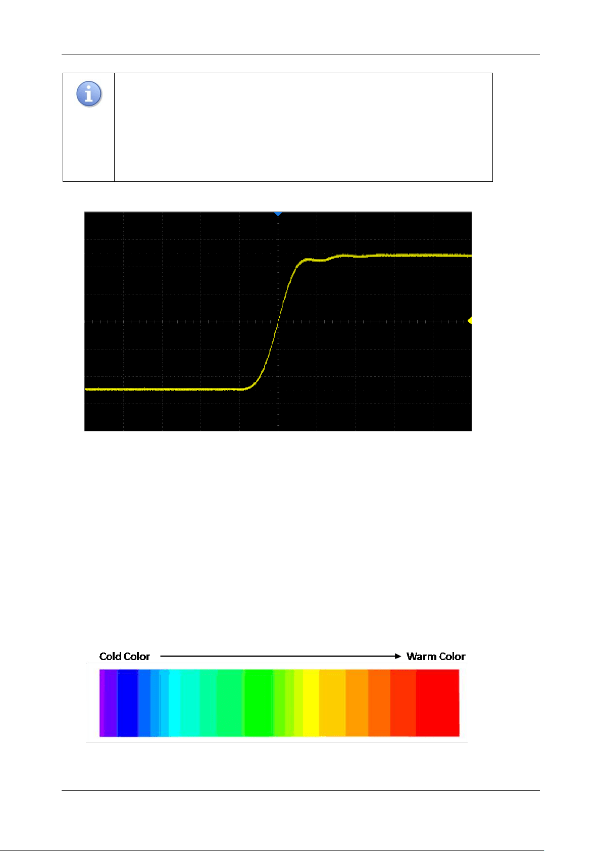
SDS6000L User Manual
int. s i g l e n t . c o m 2 7 3
Note:
In the Run state, due to the high waveform update rate of the
oscilloscope, the waveform displayed is the superposition of multiple
frames. Therefore, what is seen using the dots display is not the discrete
sampling points, but the display effect similar to equivalent sampling. Stop
the acquisition to view the original samples of each frame separately.
Dots display in Run state
Color Grade
Color grade uses color temperature to map the probability of the waveforms. The greater the probability
that the waveform appears in a pixel, the warmer the color of the pixel. The smaller probability, the
colder the color temperature of that pixel.
The picture below shows the change of color from cold to warm.
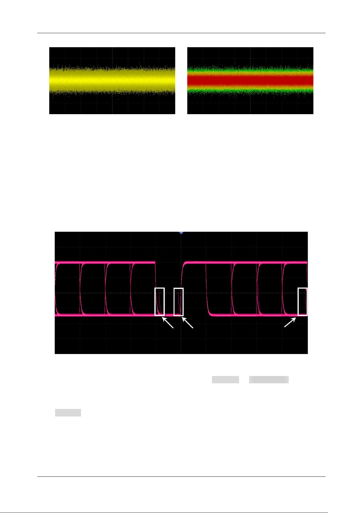
SDS6000L User Manual
2 7 4 i n t . s i g l e n t . c o m
Color grade On
Color grade Off
Set Persist
With persistence, the oscilloscope updates the display with new acquisitions but does not erase the
results of previous acquisitions in the specified period. All previous acquisitions are displayed with
reduced intensity. New acquisitions are shown in their normal color with normal intensity. In
combination with SDS6000L's high waveform update rate and persist function, in some cases
anomalies in the waveform can be found in a short time without complex trigger settings to improve
test efficiency. Below is an example to display glitches in a data sequence with infinite persistence.
When the display dialog box and persist are off, performing Display > Persistence can turn on
persist.
Click Persist in the display dialog box to set the persistence time.
Off:
Turn off persist.
Variable persist time (100ms, 200ms, 500ms, 1s, 5s, 10s, 30s):
Choose different persist
times. The oscilloscope updates with the newly acquired waveform display. Acquired
waveforms will be cleared after the corresponding time has expired.
SDS6000L User Manual
int. s i g l e n t . c o m 2 7 5
Infinite:
Select “Infinite”, previous acquisitions will never be erased until a Clear Display
operation is performed.
Set Grid
Full Grid:
Display 8*10 grid
Light Grid:
Display 2*2 grid
No Grid:
Display without grid
Full Grid
Light Grid
SDS6000L User Manual
2 7 6 i n t . s i g l e n t . c o m
No Grid
Color Setting
The color setting supports user-defined trace colors. Click the color rectangle box to set in the pop-up
palette page. Click the Default area to restore the default color for all channels.
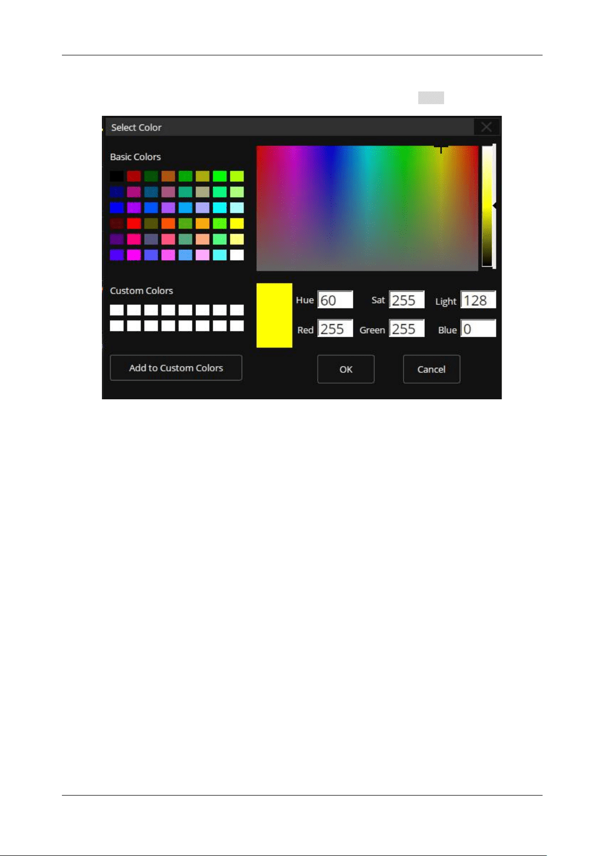
SDS6000L User Manual
int. s i g l e n t . c o m 2 7 7
Select a color directly on the palette and preview its hue, saturation, light, and RGB values or directly
modify the color parameters to customize the color. After the change, click OK to confirm.
Axis Label Setting
Turn on the axis label, the horizontal axis label will be displayed at the bottom of the grid, and the
vertical axis label will be displayed at the left of the grid. There are two display modes of the axis labels:
moving and fixed.
Moving mode:
When moving the waveform, the position of the axes moves with the waveform,
while the coordinates remain fixed.
Fixed mode:
The position of the axes remains fixed, while the coordinates update as the
waveform is moving.
SDS6000L User Manual
2 7 8 i n t . s i g l e n t . c o m
Moving mode
Fixed mode
SDS6000L User Manual
int. s i g l e n t . c o m 2 7 9
31 Waveform Generator
31.1 Overview
The SDS6000L supports waveform/function generation by incorporating a built-in Waveform Generator
accessory combined with the software activation using option SDS6000L-FG.
The AWG functions include:
6 basic waveforms: Sine, Square, Ramp, Pulse, Noise, and DC
45 built-in arbitrary waveforms
Output frequency up to 25 MHz
-3 V ~ +3 V output amplitude range
Refer to the datasheet for the detailed specifications of the AWG.
SDS6000L-FG Option
For the installation of the SDS6000L-FG option, please refer to the section "Install Option".
Click the menu Utility > AWG Menu to recall the AWG dialog box.
A. Turn on/off the output of AWG
B. Select the waveform type (Sine, Square,
Ramp, Pulse, Noise, DC, and Arb)
C. Set the frequency
D. Set the amplitude
E. Set the offset
F. Other AWG settings: Output load,
overvoltage protection, and so on.
G. AWG system information and firmware
upgrade
SDS6000L User Manual
2 8 0 i n t . s i g l e n t . c o m
31.2 Wave Type
The AWG function provides six standard waveforms and multiple arbitrary waveforms. The standard
waveforms are Sine, Square, Ramp, Pulse, Noise, and DC.
The following table shows all waveform types and corresponding parameters.
Wave Type
Parameters
Sine
Frequency, Amplitude, Offset
Square
Frequency, Amplitude, Offset, Duty
Ramp
Frequency, Amplitude, Offset, Symmetry
Pulse
Frequency, Amplitude, Offset, Duty
DC
Offset
Noise
Stdev, Mean
Arb
Frequency, Amplitude, Offset, Arb Type
The Arbitrary waveforms consist of two types: built-in waveforms and stored waveforms. Click
Arb Type in the AWG dialog box, and select the arbitrary in the pop-up window:
SDS6000L User Manual
int. s i g l e n t . c o m 2 8 1
There are 6 tabs in the window. Under each tab, a catalog of waveforms is listed. Built-in waveforms
are stored in Common, Math, Engine, Window, and Trigo. Stored waveforms are located in the Stored
menu.
Users can edit arbitrary waveforms using SIGLENT EasyWaveX PC software, send the stored
waveforms to the instrument through the remote interface, or import the stored waveforms through a
U disk.
31.3 Other Setting
Click Setting in the AWG dialog box to
recall the "Other Setting" dialog box:
A. Select the output load
B. Turn on/off the OVP (Over Voltage
Protection)
C. Do zero adjust
D. Set to default
E. Return to the previous menu
Output Load
The selected output load value must match the load impedance. Otherwise, the amplitude and offset
of the output waveform of AWG will be incorrect.
OVP
When OVP is enabled, the output will be turned off automatically once the protection condition is met.
The protection condition is when the absolute value on the output port is higher than 4 V ± 0.5 V. At
the same time, a warning message is displayed.
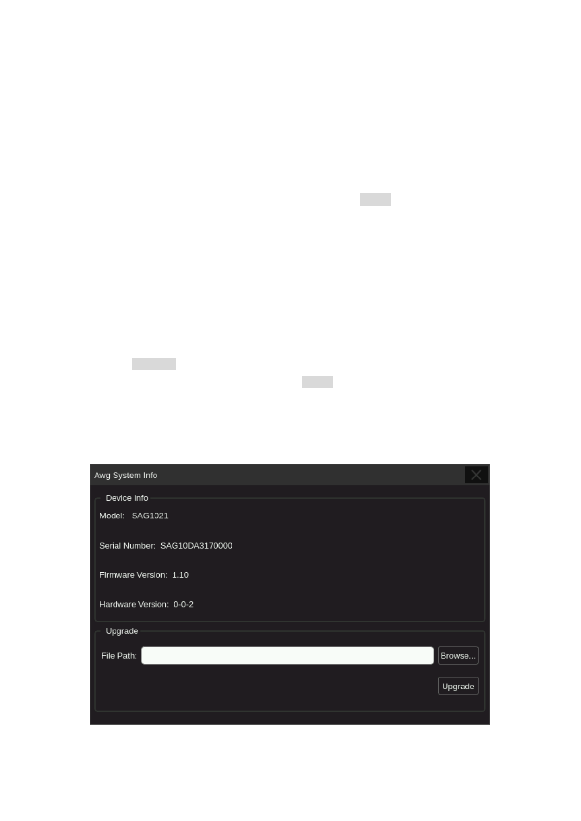
SDS6000L User Manual
2 8 2 i n t . s i g l e n t . c o m
Zero Adjust
The output zero error of the AWG can be calibrated by using auto mode or manual mode. The object
of the Zero Adjust is: when AWG outputs a 0 V DC signal, the measured mean value of the
corresponding channel is within ± 1mV.
Auto Steps
: In this mode, the adjustment can only be performed with C1 of the oscilloscope.
Connect the output of AWG to C1 of the oscilloscope, click Auto , and the AWG will start to
automatically adjust. The scope will display “Zero adjust completed!” when the adjustment is done.
Manual Steps
: The AWG can be manually calibrated through any channel on the oscilloscope.
Take C2 as an example:
1. Connect the output of AWG to C2, open C2, set it to DC coupling, turn on the bandwidth limit,
and set the probe attenuation to 1X.
2. Set the vertical scale of C2 to a small scale such as 1 mV/div. Turn on the measure and set
the parameter to the Mean of C2.
3. Click Manual and roll the mouse wheel to adjust the compensation value, until the mean
value of C2 is within ± 1 mV, and then click Save .
31.4 System
SDS6000L User Manual
int. s i g l e n t . c o m 2 8 3
Device Info
– Includes Model, Serial Number, Firmware Version, and Hardware Version of the AWG
module.
Upgrade
The firmware here refers to the firmware of the built-in AWG module. The SDS6000L supports firmware
and configuration file upgrades for the AWG via a U disk. Follow the steps below:
1. Copy the upgrade file (*.ADS) to the U disk.
2. Insert the U disk into one of the USB host ports of the oscilloscope.
3. Click Browse… to select the path of the upgrade file. See the chapter "Save/Recall" for
the detailed operation.
4. Click Upgrade to start the upgrade progress. A progress bar shows the percentage
finished.
5. After the upgrade, reboot the oscilloscope.
6. Enter the System dialog box again to check if the upgraded hardware version number is
consistent with the target version.
Warning:
Don't cut off the power during the upgrade !

SDS6000L User Manual
2 8 4 i n t . s i g l e n t . c o m
32 Save/Recall
The SDS6000L supports saving setups, reference waveforms, screenshots, and waveform data files
to internal storage, external USB storage devices (e.g. U disk), or network storage. Saved setups and
reference waveforms can be recalled as needed.
For details on network storage, refer to the section “Network Mapping”.
32.1 Save Type
The SDS6000L supports save types: Setup, Reference, Image (*.bmp/*.jpg/*.png), Waveform Data
(binary/CSV/MATLAB), and FileConverter Tool. It also supports saving the current setup as the default
setting. Here are brief descriptions of save types:
Setup
The default save type of the oscilloscope. The setup is saved with the *.xml file extension.
Reference
The reference waveform data are saved with the *.ref file extension. The saved file contains the
reference waveform data and its setup information such as the vertical scale, vertical position, and
timebase.
BMP
Saves the screenshot in *.bmp format.
JPG
Saves the screenshot in *.jpg format.
PNG
Saves the screenshot in *.png format.

SDS6000L User Manual
int. s i g l e n t . c o m 2 8 5
Binary Data
Saves the waveform data in binary (*.bin) format.
CSV Data
Saves the waveform data in ".csv" format. After selecting this type, you can click the ParaSwitch to
determine whether to include the scope configuration parameter information (horizontal timebase,
vertical scale, etc.) or not. Click the Save All Channel to save all displayed waveforms on the screen
or select the Source to save. The available sources include C1 ~ C8 and F1 ~ F4.
Matlab Data
Saves the waveform data in *.mat or *.dat format which can be imported by Matlab directly. The
available sources include C1 ~ C8 and F1 ~ F4 (except for FFT).
To Default Key
The oscilloscope provides two options for the default setting. When the Default Type is set to “Factory”,
the factory default setting will be recalled by performing Acquire > Default ; When the Default
Type is set to “Current”, the last setting saved by the “To Default Key” operation will be recalled.
FileConverter
The mini tool is used to convert stored binary files to CSV format for viewing with a spreadsheet
program. This is ideal when collecting large datasets. For a waveform frame with deep memory such
as 250 Mpts, saving directly as a CSV file will take a long time and will occupy a large amount of
memory on a USB storage device. It’s recommended to save the data as a binary file and then convert
it to a CSV file on a computer.
To Memory
This is used to save the specified source to a memory trace (M1~M4). Refer to the chapter "Memory"
for details.

SDS6000L User Manual
2 8 6 i n t . s i g l e n t . c o m
The following table shows the relationship between the save types and save/recall operations.
Type
Save to External
Recall
Setup
√
√
Reference
√
√
BMP
√
×
JPG
√
×
PNG
√
×
Binary Data
√
×
CSV Data
√
×
Matlab Data
√
×
FileConverter
√
×
Memory
√
×
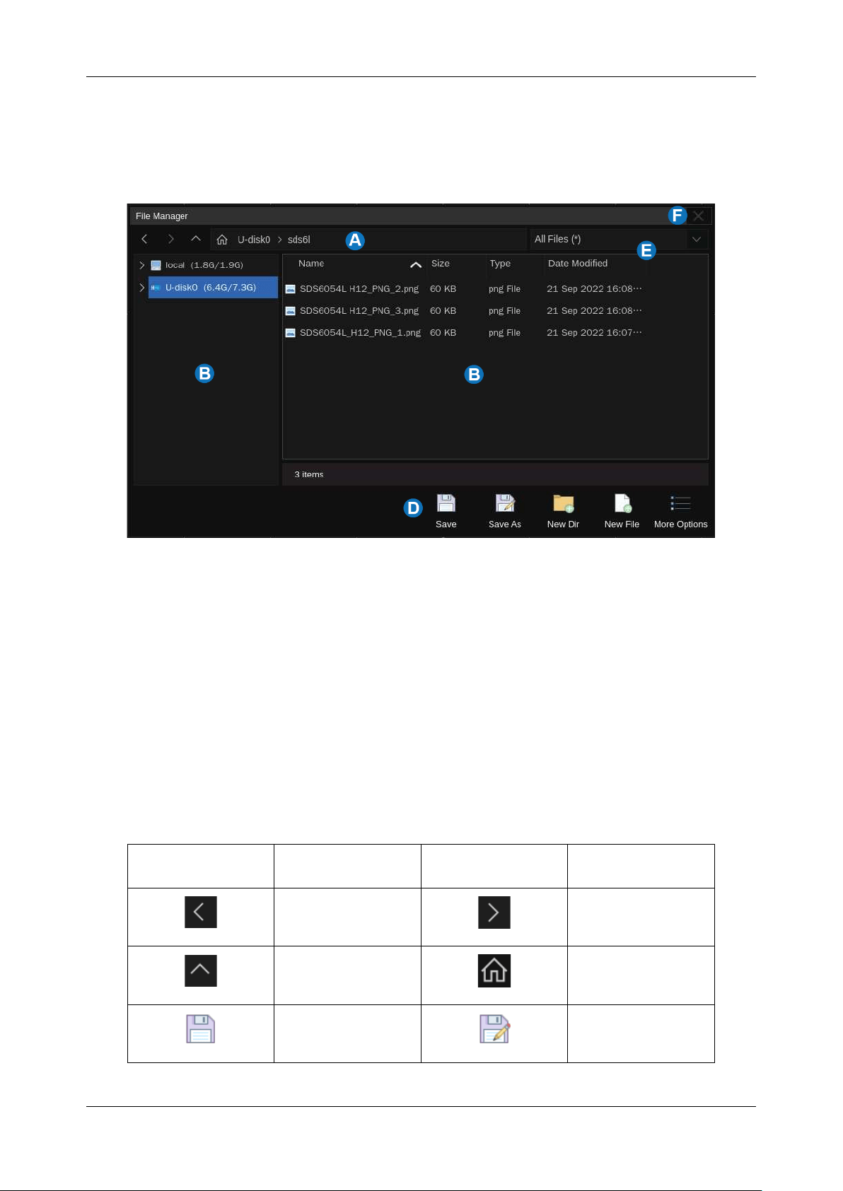
SDS6000L User Manual
int. s i g l e n t . c o m 2 8 7
32.2 File Manager
The SDS6000L's file manager has a similar style and operation to the Windows© operating systems.
A. Address bar
B. Navigation panel
C. File list
D. Toolbar
E. File type
F. Close the file manager
Table 32.1 Description of icons in the file manager
Icon
Description
Icon
Description
Back
Forward
Up level
Root directory
Save
Save as
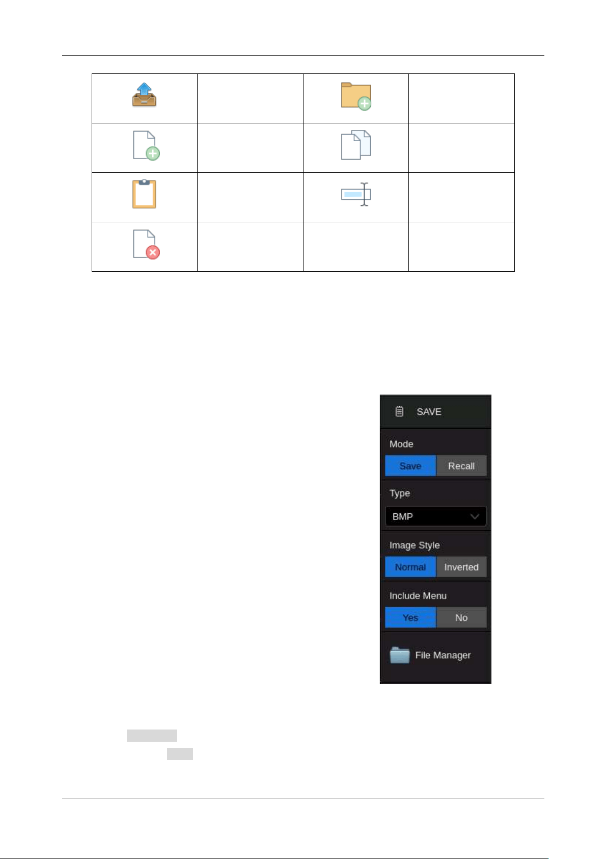
SDS6000L User Manual
2 8 8 i n t . s i g l e n t . c o m
Recall
New directory
New file
Copy
Paste
Rename
Delete
32.3 Save and Recall Instances
Save the screenshot to the path “Udisk0\sds6l\” in the format of BMP
First, Insert the U disk.
Secondly, set the parameters of the Save operation:
Select Mode as "Save"
Select Type as "BMP"
Select the Image Style. "Normal" saves
images with the same color of the display;
"Inverted" saves images with a white
background color to save ink during printing
Select to include the menu in the Print Area
or not. "No" only saves the grid area and
descriptor boxes; "Yes" saves the whole
display
Click File Manager to open the file manager
Third, select the “\Udisk0\sds6l\” directory in the file manager;
Fourth, click Save As , click the pop-up text box to recall the virtual keyboard and input the file
name, and then click OK :
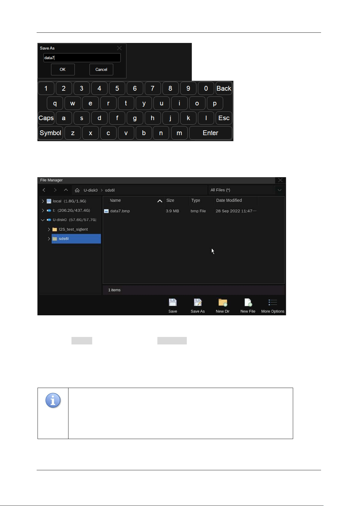
SDS6000L User Manual
int. s i g l e n t . c o m 2 8 9
Once saved, the new BMP file is visible in the file manager:
In step 4, if Save is selected instead of Save As , the system saves the file as the default file
name SDS6xxxL_BMP_n.bmp, where n is an integer incrementing from 1. The default save path is
\SIGLENT\.
Note:
When a file is saved successfully, a message will pop up to inform that
it has been saved, and the filename of the next file to be saved is shown as
well. The default naming strategy is to add an incremental number at the end
of the first saved filename.
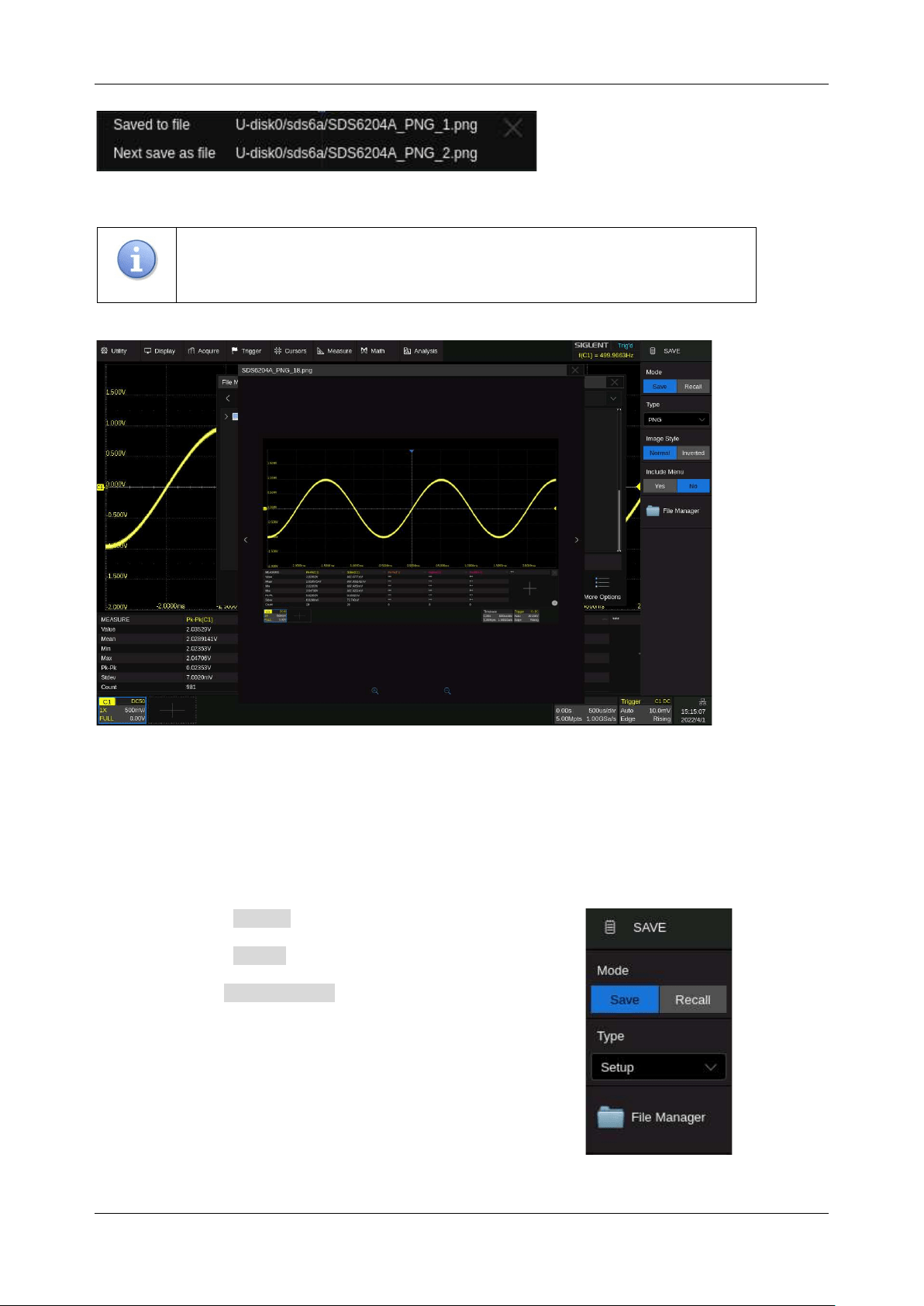
SDS6000L User Manual
2 9 0 i n t . s i g l e n t . c o m
Note:
A saved picture can be browsed on the oscilloscope by opening it in the
File Manager.
Recall the setup file " Track.xml" stored in path “Udisk0\sds6l\”
First, insert the U disk with the file " Track.xml" stored folder “\sds6l\”.
Second, set the parameters of the Recall operation:
Select Mode as "Recall"
Select Type as "Setup"
Click File Manager to open the file manager
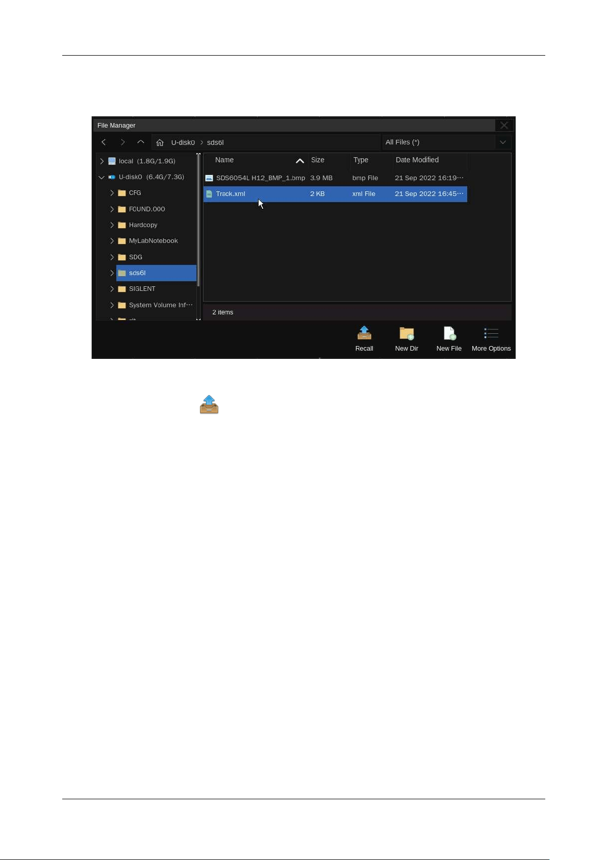
SDS6000L User Manual
int. s i g l e n t . c o m 2 9 1
Third, select the “ \Udisk0\sds6l\ ” directory in the file manager, and then select the setup file
"Track.xml"
Fourth, click the Recall icon and wait for the oscilloscope to finish recalling the setup.
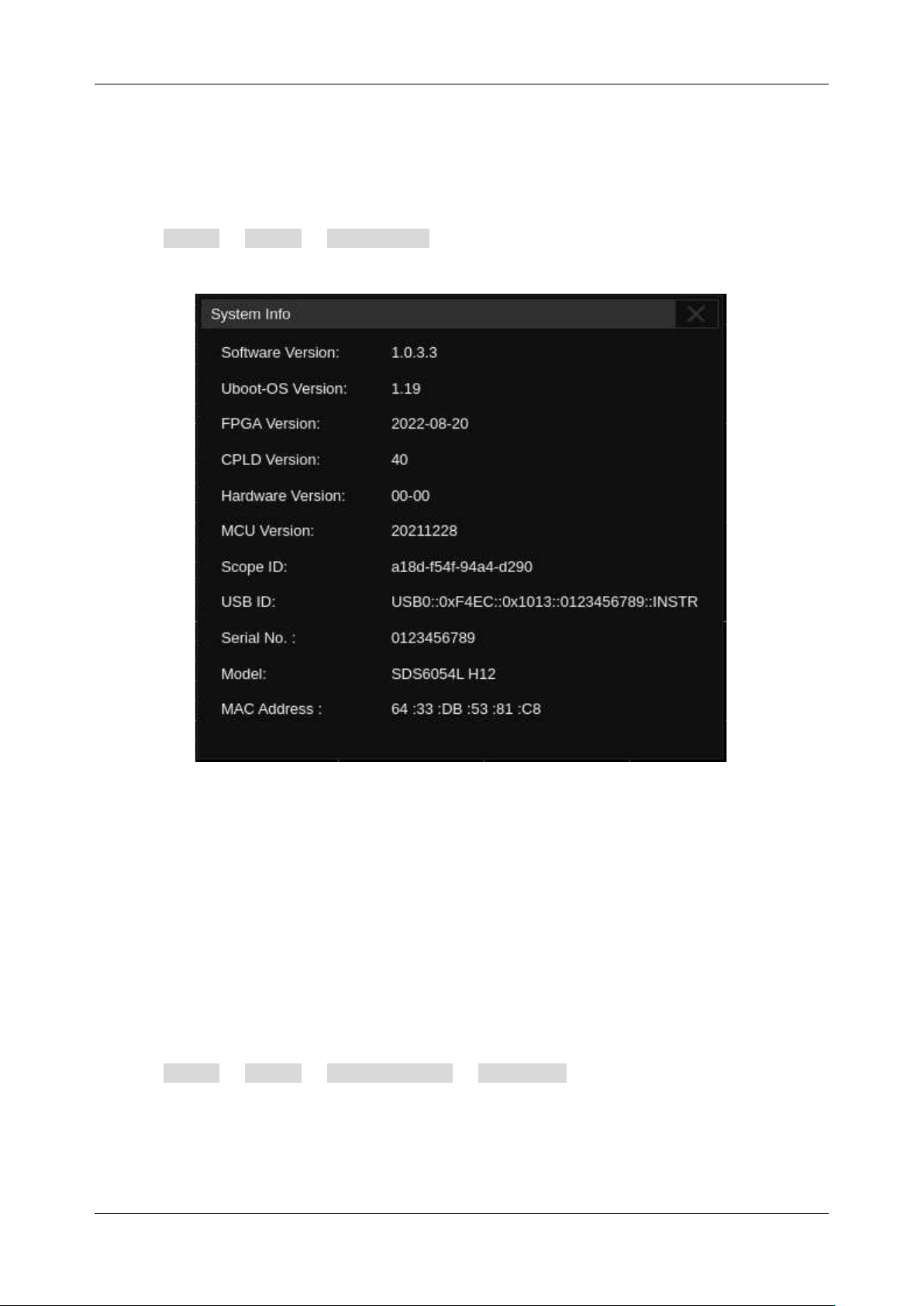
SDS6000L User Manual
2 9 2 i n t . s i g l e n t . c o m
33 Utility
33.1 System Information
Operate Utility > Menu
> System Info to check the system status. System information
includes the contents shown below.
33.2 System Setting
33.2.1 Language
The SDS6000L supports multiple languages, including Simplified Chinese, Traditional Chinese,
English, French, Japanese, German, Spanish, Russian, Italian, Portuguese, and so on.
Operate Utility > Menu > System Setting > Language , and select the language in the
list.

SDS6000L User Manual
int. s i g l e n t . c o m 2 9 3
33.2.2 Screen Saver
The screen saver will be activated if the oscilloscope has not been operated for a period. At this time
the output of the display is cut off to save power consumption.
Operate Utility > Menu > System Setting > Screen Saver to specify the period before the
screen saver activates, or select "Off" to disable the screen saver.
Any action from the mouse, web control, or front panel can trigger to exit the screen saver.
33.2.3 Sound
Follow the steps Utility > Menu > System Setting > Beeper to enable or disable the
audible buzzer.
33.2.4 Auto Power-on
Operate Utility > Menu > System Setting > Auto Power On to set. See the chapter
“Mechanical Dimension” for details.
33.2.5 Date/Time
The SDS6000L has an RTC clock, which helps to record absolute time information for screenshots,
history frames, and so on.
Operate Utility > Menu > System Setting > Date/Time to open the Date/Time dialog box:
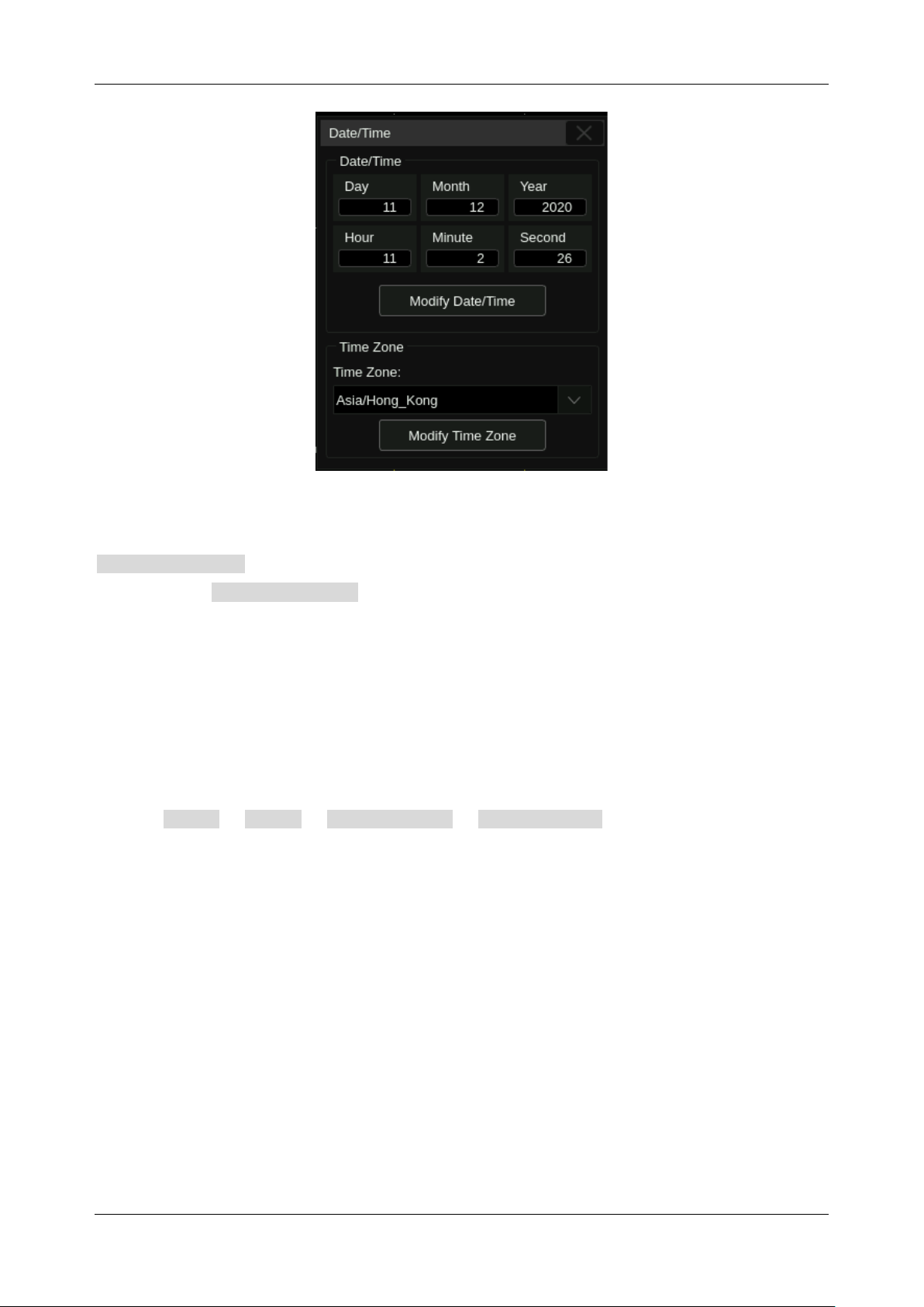
SDS6000L User Manual
2 9 4 i n t . s i g l e n t . c o m
Click the text box of Hour, Minute, Second, Day, Month, and Year to edit these fields. Click the
Modify Date/ Time button to perform the change. Click the text box of Time Zone to select the time
zone. Click the Modify Time Zone button to perform the change.
33.2.6 Reference Position Setting
The reference position is used to set the strategy of scaling on the horizontal and vertical axes,
adapting to different requirements.
Operate Utility > Menu > System Setting > Reference Pos to open the dialog box, and
choose the strategy for the offset value change in the vertical (or horizontal) direction when the
vertical (or horizontal) scale is changed.
Horizontal Ref
Fixed Delay:
When the time base is changed, the horizontal delay value remains fixed. As
the horizontal timebase scale is changed, the waveform expands/contracts around the
center of the display
Fixed Position:
When the time base is changed, the horizontal delay remains fixed to the
grid position on the display. As the horizontal time base scale is changed, the waveform
expands/contracts around the position of the horizontal display.
SDS6000L User Manual
int. s i g l e n t . c o m 2 9 5
Vertical Ref
Fixed Offset:
When the vertical scale is changed, the vertical offset remains fixed. As the
vertical scale is changed, the waveform expands/contracts around the main X-axis of the
display
Fixed Position:
When the vertical scale is changed, the vertical offset remains fixed to the
grid position on the display. As the vertical scale is changed, the waveform expands/contracts
around the position of the vertical ground position on the display.
Take Horizontal Ref as an example to demonstrate the scaling effect of different settings:
Timebase = 10 ns/div, Horizontal Delay = -20 ns = - 2 div
SDS6000L User Manual
2 9 6 i n t . s i g l e n t . c o m
Fixed position, timebase is changed to 5 ns/div, the grid number of delay (-2div) remains
fixed, while the horizontal delay changes to -10 ns
Fixed delay, timebase is changed to 5 ns/div, the horizontal delay value remains fixed,
while the grid number of delay changes to -4div
SDS6000L User Manual
int. s i g l e n t . c o m 2 9 7
33.2.7 Tips
When a file is saved successfully, a message will pop up to inform the user that the image has been
saved. The Message box status can be set as shown below:
Operate Utility > Menu > System Setting > Tips to open the tips dialog box:
Hold:
The message box will remain at the
top of the waveform display area.
Fade:
The message box will disappear
automatically after the set time, and the
time range is: 0.1~9.9s.
None:
The message box will not pop up.
33.3 I/O Setting
33.3.1 LAN
Operate the following steps to set the LAN port:
Perform
Utility
> I/O > LAN Config to open the LAN Config dialog box.
SDS6000L User Manual
2 9 8 i n t . s i g l e n t . c o m
A. Check Automatic to enable dynamic IP. In
this case, the oscilloscope must be connected
to the local area network with a DHCP server.
Contact your network administrator to confirm
the relevant information.
B. When is not checked, the oscilloscope
uses static IP. Set the static IP address,
subnet mask, and gateway separately.
C. If your network provides Dynamic DNS, you
can enable Automatic (DNS) to let the
oscilloscope register its hostname and use the
DNS server for name resolution.
D. When is not checked, set the DNS IP
address manually.
E. When accessing more than two SIGLENT
instruments through the web browser, it is
necessary to set a different VNC port number
for each instrument. The range is from 5900 to
5999.
33.3.2 Clock Source
The clock source of the device can be set to "Internal" or "External". When the clock source is set to
"external", the device receives the 10 MHz clock from the "10 MHz In" port on the rear panel and uses
it as a reference to generate the sampling clock of the system. Both “internal" and "external" clock
sources can be output from the 10 MHz Out port for synchronizing other instruments.
When the clock source is set to "External", an icon indicating an external clock will appear in the lower
right corner of the display:
The clock source is external.
The clock source is external, but no valid external clock is detected.
SDS6000L User Manual
int. s i g l e n t . c o m 2 9 9
33.4 Install Options
The SDS6000L provides a few options to enhance its functionality. Contact your local
SIGLENT
sales
representative or
SIGLENT
technical support to get the corresponding option key. Perform the
following steps to install the option:
Utility > Menu > Software Options
A. Option information display area. When the option is not activated, the license type is displayed as
"Temporary" and can be tried up to 30 times.
B. Select the option to install.
C. The option key input area, click the text box, and enter the key by the virtual keyboard.
D. Clear the characters in the key input area.
E. After entering the option key, click Install to perform the installation.
F. Use the U-disk to automatically install the option, the license must be stored in the root directory
of the U-disk.
SDS6000L User Manual
3 0 0 i n t . s i g l e n t . c o m
33.5 Maintenance
33.5.1 Upgrade
The firmware is upgradeable through an external USB memory device/U disk. Make sure the U disk
contains the correct upgrade file (*.ads) and is connected to the oscilloscope before performing the
upgrade.
Operate Utility > Menu > Maintenance > Upgrade to recall the upgrade dialog box:
Click Browse to open the file manager, select the correct upgrade file and click the Recall icon .
SDS6000L User Manual
int. s i g l e n t . c o m 3 0 1
Click Upgrade in the upgrade dialog box to start the upgrade. The oscilloscope first copies the
upgrade file (*.ads) to the local memory and parses it. If the parse succeeds, it will show the following
dialog. Users can choose Cancel to cancel the upgrade or Reboot to restart the oscilloscope
immediately and continue the upgrade. Otherwise, the oscilloscope will restart automatically to finish
the upgrade.
After the reboot, check if the version number is in the "Information System".
Warning:
Do not turn off the power during upgrading. Otherwise, the
oscilloscope may not boot up!
33.5.2 Self-Calibration
The self-calibration program can quickly calibrate the oscilloscope to reach the best working state and
the most precise measurement. It is recommended to perform a self-calibration if the change of ambient
temperature is more than 5
℃
.
Note:
Make sure the oscilloscope has been warmed up or operated for more
than 30 minutes before the self-calibration.
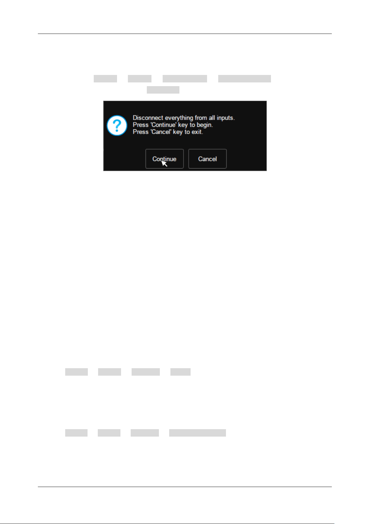
SDS6000L User Manual
3 0 2 i n t . s i g l e n t . c o m
Please do the self-calibration as follows:
1. Disconnect everything from all inputs.
2. Operate Utility > Menu > Maintenance > Self Calibration , and the following
dialog box appears. Select Continue to start the self-cal program.
3. The oscilloscope will not respond to any operation until the self-cal is finished. After the self-
cal is completed, click the screen to exit.
33.5.3 Developer Options
This function is used for internal development by
SIGLENT
.
33.6 Service
33.6.1 Web
The SDS6000L includes a web server function, you can access and control the oscilloscope using a
web browser. See the section "Web Browser" for details about remote control.
Perform Utility > Menu > Service > Web to set the password to control the instrument.
The password length is limited to 20 bytes.
33.6.2 Network Mapping
Perform Utility > Menu > Service > Network Mapping to open the network mapping dialog
box:
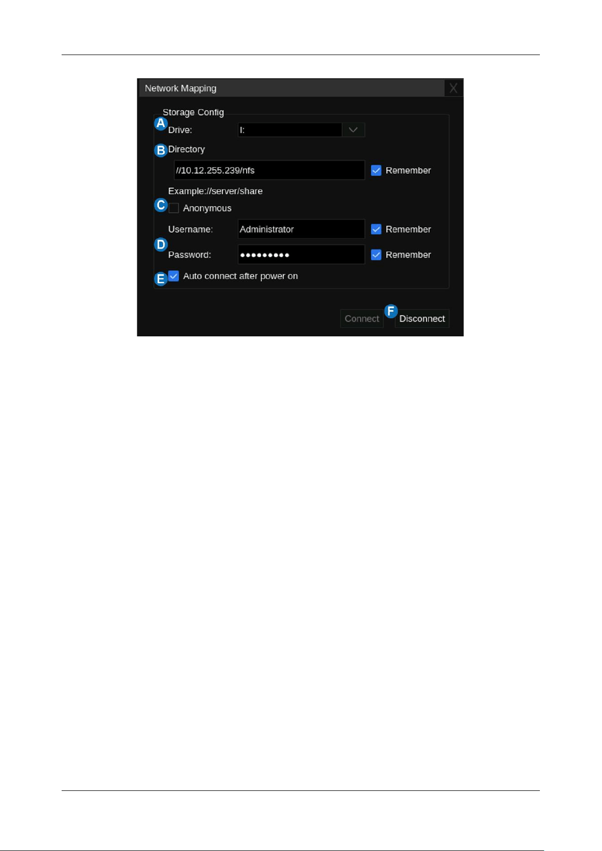
SDS6000L User Manual
int. s i g l e n t . c o m 3 0 3
A. Network mapped drive letter. The default is I:
B. Input the network storage directory in the text box. Check “Remember” to
remember it.
C. Check
“
Anonymous
”
to access the network directory in guest mode (Username:
Guest, no password). This needs the server to permit anonymous access.
D. Username and password. Check “Remember” to save them.
E. Check to automatically connect to the network directory at every power on.
F. Connect or disconnect to the network directory manually.
33.6.3 Emulation
When the “Emulation” option is set to “Tektronix”, the SCPI command set of the instrument is changed
to be compatible with Tek. This setting can help the user switch from a Tek scope with minimum
changes to the existing code.
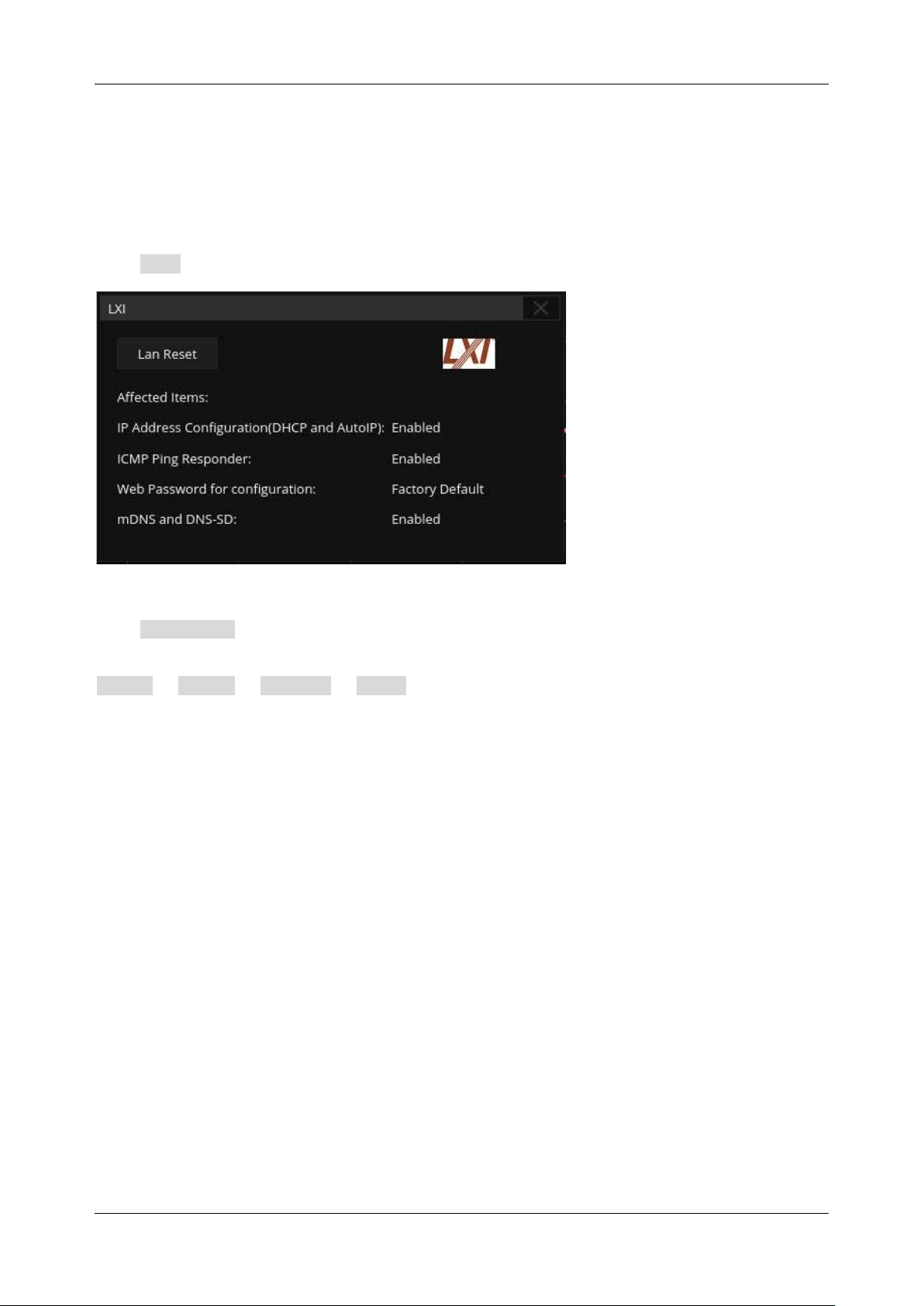
SDS6000L User Manual
3 0 4 i n t . s i g l e n t . c o m
33.6.4 LXI
This oscilloscope complies with LXI version 1.5, defined in LXI device specification 2016, which can
be used to quickly build automated test systems.
Click LXI to recall the LXI status box as below:
Click LAN Reset to restore the LAN defaults to your oscilloscope. It will enable automatic IP,
ICMP Ping responder, and Multicast DNS, and reset the webserver password which is set in
Utility > Menu > Service > Web .
After setting the LAN, the LXI welcome page can be loaded through the browser, refer to the section
“LAN” and “Web Browser” for details. When starting instrument identification in the web server, the
LXI image in the upper right corner will flash continuously.
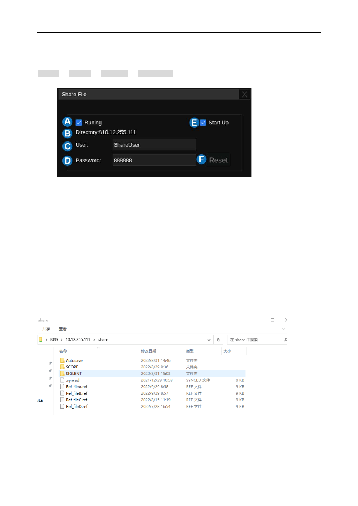
SDS6000L User Manual
int. s i g l e n t . c o m 3 0 5
33.6.5 Share File
After setting the shared file, you can access the internal files of the device through Windows. Perform
Utility > Menu > Service > Share File to open the share file dialog box:
A. Set the working status of the share file.
B. The share directory IP address (same as the device IP address)
C. Username. The default is ShareUser and cannot be changed.
D. Password. It can only be modified when sharing is stopped.
E. Check to automatically start up the share file at every power on.
F. Check to reset share file.
After running the service, enter the shared file of the access device under Windows:
SDS6000L User Manual
3 0 6 i n t . s i g l e n t . c o m
34 Troubleshooting
The commonly encountered failures and their solutions are listed below. When you encounter those
problems, please solve them using the corresponding steps. If the problem remains, please contact
SIGLENT
as soon as possible.
1. The screen is still dark (no display) after power on:
1) Check whether the power is correctly connected.
2) Check whether the power switch is on.
3) Check whether the fuse is burned out. If the fuse needs to be changed, please contact
SIGLENT
timely and return the instrument to the factory for replacement by the
maintenance personnel authorized by
SIGLENT
.
4) Restart the instrument after finishing the above inspections.
5) If it still does not work correctly, please contact
SIGLENT
.
Note:
It takes up to 1 minute from power on to display an image on an
external monitor.
2. The signal is sampled but no waveform of the signal is displayed:
1) Check whether the probe is correctly connected to the signal connecting wire.
2) Check whether the signal connecting wire is correctly connected to the BNC (namely
channel connector).
3) Check whether the probe is correctly connected to the item to be tested.
4) Check whether there are signals generated from the item to be tested.
5) Resample the signal.
3. The tested voltage amplitude is greater or lower than the actual value (Note that this problem
usually occurs when the probe is used):
1) Check whether the attenuation coefficient of the channel complies with the attenuation
ratio of the physical probe.
2) Disconnect the oscilloscope from the external signal and do a self-cal.

SDS6000L User Manual
int. s i g l e n t . c o m 3 0 7
4. There is a waveform display but not stable:
1) Check the trigger signal source: check whether the source item at the trigger panel
complies with the signal channel used.
2) Check whether it is a "false wave”: when the signal frequency is very large (more than
half of the sample rate), it is easy to appear as a "false wave". At this point, a small
timebase should be set to make the sample rate more than 2 times the signal frequency.
3) Check the trigger type: general signals should use the “Edge” trigger and video signals
should use the “Video” trigger. Only when the proper trigger type is used, can the
waveform be displayed stably.
4) Change the trigger holdoff setting.
5. No display after performing Acquire > Run :
Check whether the mode at the trigger panel (TRIGGER) is on “Normal” or “Single” and whether
the trigger level exceeds the waveform range. If yes, set the trigger level to the middle or set the
mode to “Auto”.
6. The USB storage device cannot be recognized:
1) Check whether the USB storage device can work normally.
2) Make sure the USB interface can work normally.
3) Make sure that the USB storage device being used is a flash storage type. This
oscilloscope does not support hardware storage type.
4) Make sure that the U disk system format is FAT32.
5) Restart the instrument and then insert the USB storage device to check it.
6) If the USB storage device still cannot be used normally, please contact
SIGLENT
.

About SIGLENT
SIGLENT is an international high-tech company, concentrating on R&D, sales,
production and services of electronic test & measurement instruments.
SIGLENT first began developing digital oscilloscopes independently in 2002.
After more than a decade of continuous development, SIGLENT has extended
its product line to include digital oscilloscopes, isolated handheld
oscilloscopes, function/arbitrary waveform generators, RF/MW signal
generators, spectrum analyzers, vector network analyzers, digital multimeters,
DC power supplies, electronic loads and other general purpose test
instrumentation. Since its first oscilloscope was launched in 2005, SIGLENT
has become the fastest growing manufacturer of digital oscilloscopes. We
firmly believe that today SIGLENT is the best value in electronic test &
measurement.
Headquarters:
SIGLENT Technologies Co., Ltd
Add: Bldg No.4 & No.5, Antongda Industrial
Zone, 3rd Liuxian Road, Bao'an District,
Shenzhen, 518101, China
Tel: + 86 755 3688 7876
Fax: + 86 755 3359 1582
Email: sales@siglent.com
Website: int.siglent.com
North America:
SIGLENT Technologies America, Inc
6557 Cochran Rd Solon, Ohio 44139
Tel: 440-398-5800
Toll Free: 877-515-5551
Fax: 440-399-1211
Email: info@siglentna.com
Website: www.siglentna.com
Europe:
SIGLENT Technologies Germany GmbH
Add: Staetzlinger Str. 70
86165 Augsburg, Germany
Tel: +49(0)-821-666 0 111 0
Fax: +49(0)-821-666 0 111 22
Email: info-eu@siglent.com
Website: www.siglenteu.com
Follow us on
Facebook: SiglentTech