Bang & Olufsen BEOGRAM 4000C A Classic. Reborn. User Manual

Beogram 4000c

Technical Sound Guide

Bang & Olufsen A/S

This manual is for information purposes only and is not legally binding.

May 23, 2022

Contents
History 4
1 The mechanical phonograph . . . . . . . . . . . . . . . . . . . . . . . . . . . . . . . . . . . . . . . . . . . . . . . . . 4
2 Magnets and Coils . . . . . . . . . . . . . . . . . . . . . . . . . . . . . . . . . . . . . . . . . . . . . . . . . . . . . . . 4
The physics 5
1 Amplitude vs. Velocity . . . . . . . . . . . . . . . . . . . . . . . . . . . . . . . . . . . . . . . . . . . . . . . . . . . . 5
2 Surface noise . . . . . . . . . . . . . . . . . . . . . . . . . . . . . . . . . . . . . . . . . . . . . . . . . . . . . . . . . . 5
3 Mono to Stereo . . . . . . . . . . . . . . . . . . . . . . . . . . . . . . . . . . . . . . . . . . . . . . . . . . . . . . . . 6
The cartridge , stylus, and tonearm 8
1 MMC: Micro Moving Cross . . . . . . . . . . . . . . . . . . . . . . . . . . . . . . . . . . . . . . . . . . . . . . . . . . . 8
2 Signal Levels . . . . . . . . . . . . . . . . . . . . . . . . . . . . . . . . . . . . . . . . . . . . . . . . . . . . . . . . . . 9
3 Tip shape . . . . . . . . . . . . . . . . . . . . . . . . . . . . . . . . . . . . . . . . . . . . . . . . . . . . . . . . . . . . 11
4 Bonded vs. Nude . . . . . . . . . . . . . . . . . . . . . . . . . . . . . . . . . . . . . . . . . . . . . . . . . . . . . . . 13
5 Tracking force . . . . . . . . . . . . . . . . . . . . . . . . . . . . . . . . . . . . . . . . . . . . . . . . . . . . . . . . . 14
6 Eﬀective Tip Mass . . . . . . . . . . . . . . . . . . . . . . . . . . . . . . . . . . . . . . . . . . . . . . . . . . . . . . . 14
7 Compliance . . . . . . . . . . . . . . . . . . . . . . . . . . . . . . . . . . . . . . . . . . . . . . . . . . . . . . . . . . 14
8 Soundsmith SMMC20CL . . . . . . . . . . . . . . . . . . . . . . . . . . . . . . . . . . . . . . . . . . . . . . . . . . . 15
9 Tangential Tracking . . . . . . . . . . . . . . . . . . . . . . . . . . . . . . . . . . . . . . . . . . . . . . . . . . . . . . 15
Audio Speciﬁcat ions 17
0.1 Magnitude Response . . . . . . . . . . . . . . . . . . . . . . . . . . . . . . . . . . . . . . . . . . . . . . . . . . . 17
0.2 Rumble . . . . . . . . . . . . . . . . . . . . . . . . . . . . . . . . . . . . . . . . . . . . . . . . . . . . . . . . . . . 17
0.3 Rotational speed . . . . . . . . . . . . . . . . . . . . . . . . . . . . . . . . . . . . . . . . . . . . . . . . . . . . . . 17
0.3.1 Accuracy . . . . . . . . . . . . . . . . . . . . . . . . . . . . . . . . . . . . . . . . . . . . . . . . . . . . . 17
0.3.2 Stability . . . . . . . . . . . . . . . . . . . . . . . . . . . . . . . . . . . . . . . . . . . . . . . . . . . . . 17
0.3.3 Measurement and Weighting . . . . . . . . . . . . . . . . . . . . . . . . . . . . . . . . . . . . . . . . . . 18
0.3.4 Expressing the result . . . . . . . . . . . . . . . . . . . . . . . . . . . . . . . . . . . . . . . . . . . . . . 19
Reading the measurement datasheet 20
1 Measurements from Vinyl . . . . . . . . . . . . . . . . . . . . . . . . . . . . . . . . . . . . . . . . . . . . . . . . . . . 20
1.1 Magnitude Response . . . . . . . . . . . . . . . . . . . . . . . . . . . . . . . . . . . . . . . . . . . . . . . . . . . 20
1.2 Channel Matching . . . . . . . . . . . . . . . . . . . . . . . . . . . . . . . . . . . . . . . . . . . . . . . . . . . . 21
1.3 Crosstalk . . . . . . . . . . . . . . . . . . . . . . . . . . . . . . . . . . . . . . . . . . . . . . . . . . . . . . . . . . 21
1.4 Rumble . . . . . . . . . . . . . . . . . . . . . . . . . . . . . . . . . . . . . . . . . . . . . . . . . . . . . . . . . . . 21
1.5 Wow and Flutter . . . . . . . . . . . . . . . . . . . . . . . . . . . . . . . . . . . . . . . . . . . . . . . . . . . . . . 21
1.6 Frequency Drift . . . . . . . . . . . . . . . . . . . . . . . . . . . . . . . . . . . . . . . . . . . . . . . . . . . . . . 22
2 RIAA Preampliﬁer . . . . . . . . . . . . . . . . . . . . . . . . . . . . . . . . . . . . . . . . . . . . . . . . . . . . . . . 22
2.1 Magnitude Response Deviation . . . . . . . . . . . . . . . . . . . . . . . . . . . . . . . . . . . . . . . . . . . . . 22
2.2 Channel Matching . . . . . . . . . . . . . . . . . . . . . . . . . . . . . . . . . . . . . . . . . . . . . . . . . . . . 22
Beogram 40 0 0 c Speciﬁcations 24
Further Reading 25
2

History

1.1 The mechanical

phonograph

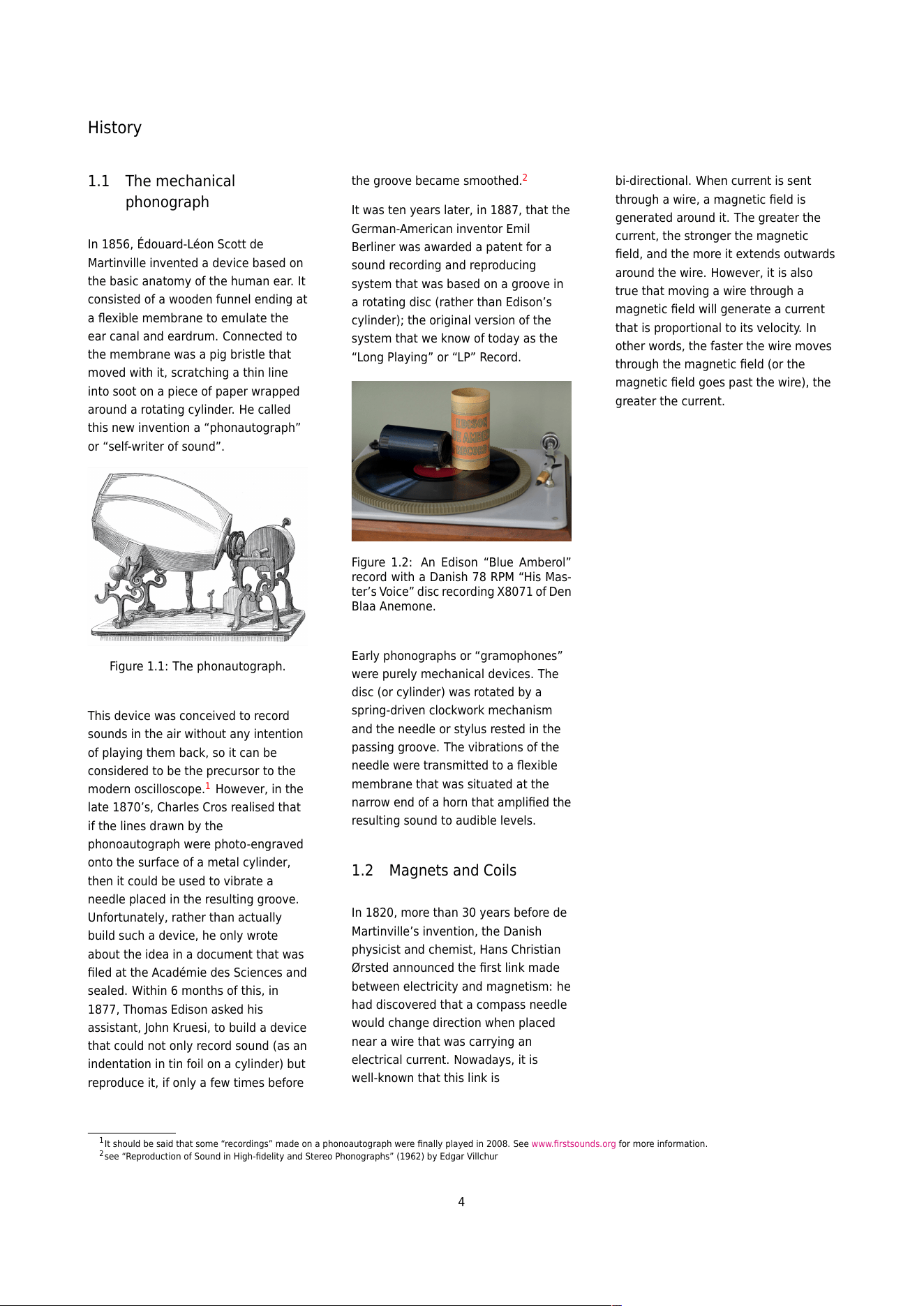
In 1856, Édouard-Léon Scott de

Martinville invented a device based on

the basic anatomy of the human ear. It

consisted of a wooden funnel ending at

a ﬂexible membrane to emulate the

ear canal and eardrum. Connected to

the membrane was a pig bristle that

moved with it, scratching a thin line

into soot on a piece of paper wrapped

around a rotating cylinder. He called

this new invention a “phonautograph”

or “self-writer of sound”.

Figure 1.1: The phonautograph.

This device was conceived to record

sounds in the air without any intention

of playing them back, so it can be

considered to be the precursor to the

modern oscilloscope.

However, in the

late 1870’s, Charles Cros realised that

if the lines drawn by the

phonoautograph were photo-engraved

onto the surface of a metal cylinder,

then it could be used to vibrate a

needle placed in the resulting groove.

Unfortunately, rather than actually

build such a device, he only wrote

about the idea in a document that was

ﬁled at the Académie des Sciences and

sealed. Within 6 months of this, in

1877, Thomas Edison asked his

assistant, John Kruesi, to build a device

that could not only record sound (as an

indentation in tin foil on a cylinder) but

reproduce it, if only a few times before

the groove became smoothed.

It was ten years later, in 1887, that the

German-American inventor Emil

Berliner was awarded a patent for a

sound recording and reproducing

system that was based on a groove in

a rotating disc (rather than Edison’s

cylinder); the original version of the

system that we know of today as the

“Lon g Playing” or “LP” Record.

Figure 1.2: An Edison “Blue Ambe rol”

record with a Danish 78 RPM “His Mas-

ter’s Voice” disc recording X8071 of Den

Blaa Anemone.

Early phonographs or “gramophones”

were purely mechanical devices. The

disc (or cylinder) was rotated by a

spring-driven clockwork mechanism

and the needle or stylus rested in the

passing groove. The vibratio ns of the

needle were transmitted to a ﬂexible

membrane that was situated at the

narrow end of a horn that ampliﬁed the

resulting sound to audible levels.

1.2 Magnets and Coils

In 1820, more than 30 years before de

Martinville’s invention, the Danish

physicist and chemist, Hans Christian

Ørsted announced the ﬁrst link made

between electricity and magnetism: he

had discovered that a compass needle

would change direction when placed

near a wire that was carrying an

electrical current. Nowadays, it is

well-known that this link is

bi-directional. When cu rrent is sent

through a wire, a magnetic ﬁeld is

generated around it. The greater the

current, the stronger the magnetic

ﬁeld, and the more it extends outwards

around the wire. However, it is also

true that moving a wire through a

magnetic ﬁeld will generate a current

that is proportional to its velocity. In

other words, the faster the wire moves

through the magnetic ﬁeld (or the

magnetic ﬁeld goes past the wire), the

greater the current.

It should be said that some “recordings” made on a phonoautograph were ﬁnally played in 2008. See www.ﬁrstsounds.org for more information.

see “Reproduction of Sound in High-ﬁdelity and Stereo Phonographs” (1962) by Edgar Villchur

The physics

2.1 Amplitude vs. Velocity

It is this second interaction that is at

the heart of almost every modern

turntable. As the stylus (or “needle”

)

is pulled through the grove in the vinyl

surface, it moves from side-to-side at a

varying speed called the modulation

velocity or just the velocity. An

example of this wavy groove can be

seen in the photo in Figure 2.1. Inside

the housing of most cartridges are

small magnets and coils of wire, either

of which is being moved by the stylus

as it vibrates. That movement

generates an electrical current that is

analogous to the shape of the groove:

the higher the velocity of the stylus,

the higher the electrical signal from

the cartridge.

Figure 2.1 : The groove in a late-1980’s

pop tune on a 33 1/3 RPM stereo LP. The

white dots in the groove are dirt that

should be removed before playing the

disc.

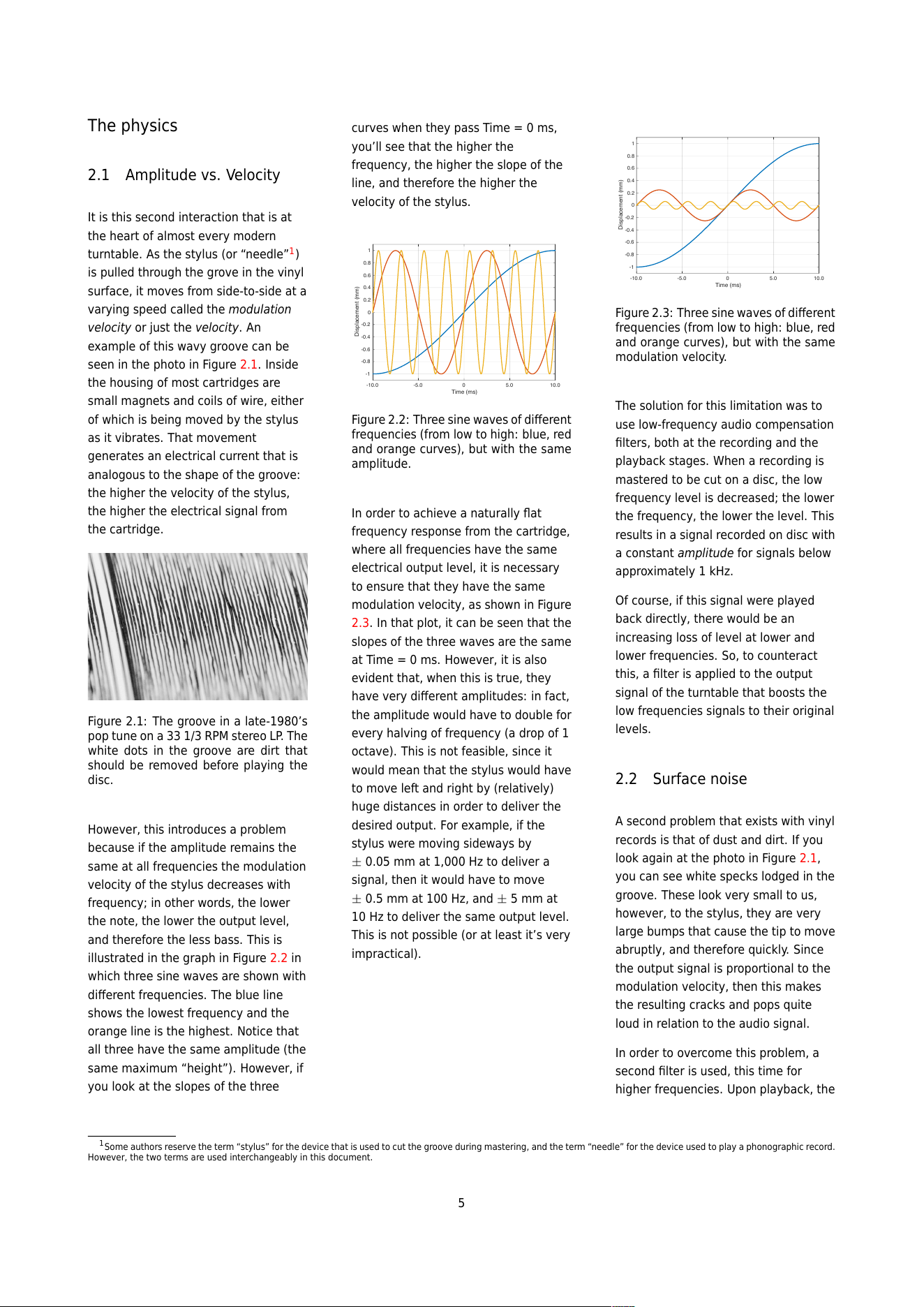
However, this introduces a problem

because if the amplitude remains the

same at all frequencies the modulation

velocity of the stylus decreases with

frequency; in other words, the lower

the note, the lower the output level,

and therefore the less bass. This is

illustrated in the graph in Figure 2.2 in

which three sine waves are shown with

diﬀerent frequencies. The blue line

shows the lowest frequency and the

orange line is the highest. Notice that

all three have the same amplitude (the

same maximum “height”). However, if

you look at the slopes of the three

curves when they pass Time = 0 ms,

you’ll see that the higher the

frequency, the higher the slope of the

line, and therefore the higher the

velocity of the stylus.

-10.0 -5.0 0 5.0 10.0

Time (ms)

-1

-0.8

-0.6

-0.4

-0.2

0.2

0.4

0.6

0.8

Displacement (mm)

Figure 2.2: Three sine waves of diﬀerent

frequencies (from low to high: blue, red

and orange curves), but with the same

amplitude.

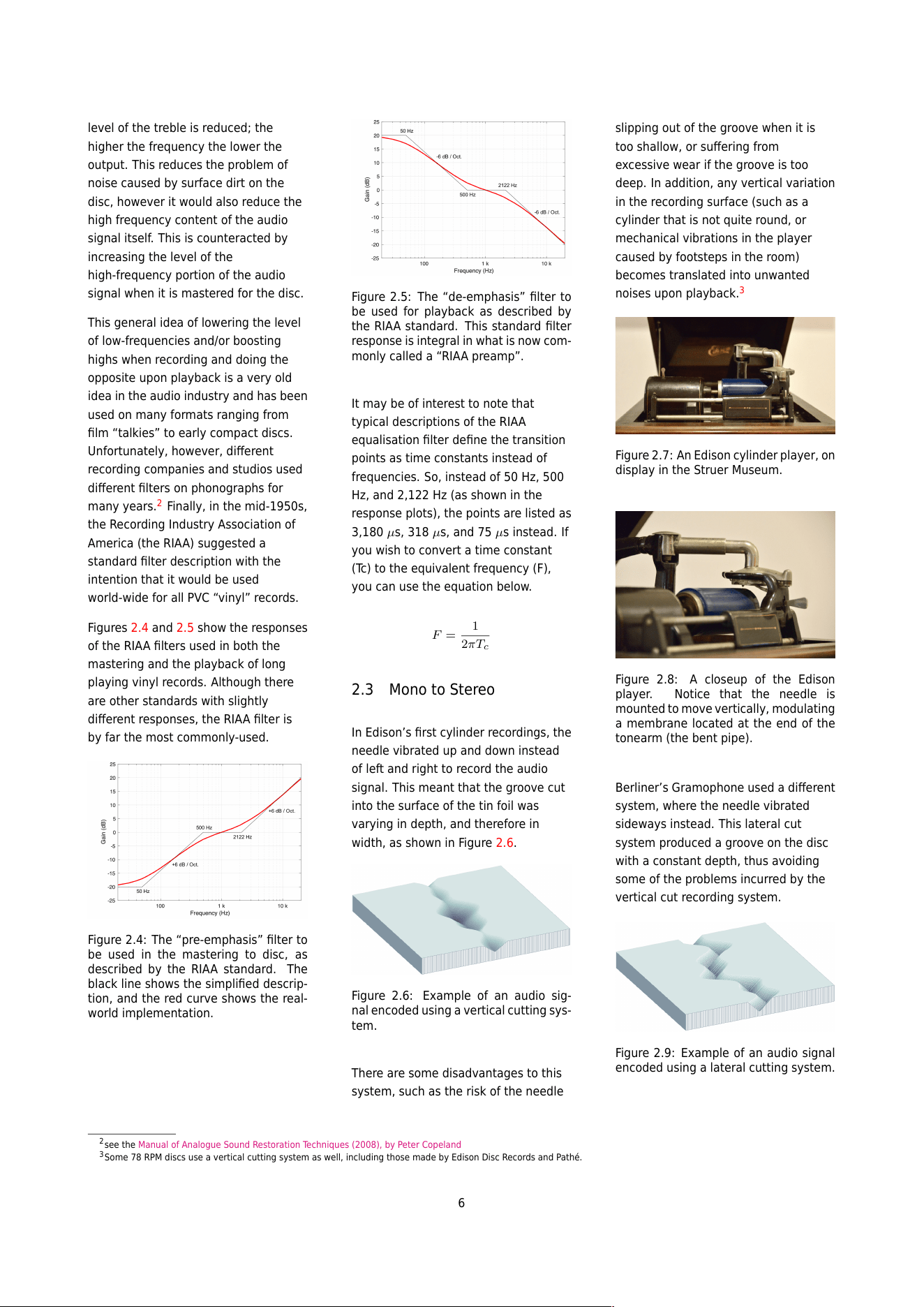
In order to achieve a naturally ﬂat

frequency response from the cartridge,

where all frequencies have the same

electrical output level, it is necessary

to ensure that they have the same

modulation velocity, as shown in Figure

2.3. In that p lot, it can be seen that the

slopes of the three waves are the same

at Time = 0 ms. However, it is also

evident that, when this is true, they

have very diﬀerent amplitudes: in fact,

the amplit ude would have to double for

every halving of frequency (a drop of 1

octave). This is not feasible, since it

would mean that the stylus would have

to move left and right by (relatively)

huge distances in order to deliver the

desired output. For example, if the

stylus were moving sideways by

± 0.05 mm at 1,000 Hz to deliver a

signal, then it would have to move

± 0.5 mm at 100 Hz, and ± 5 mm at

10 Hz to deliver the same output level.

This is not possible (or at least it’s very

impractical).

-10.0 -5.0 0 5.0 10.0

Time (ms)

-1

-0.8

-0.6

-0.4

-0.2

0.2

0.4

0.6

0.8

Displacement (mm)

Figure 2.3: Three sine waves of diﬀerent

frequencies (from low to high: blue, red

and orange curves), but with the same

modulation velocity.

The solution for this limitation was to

use low-frequency audio compensation

ﬁlters, both at the recording and the

playback stages. When a recording is

mastered to be cut on a disc, the low

frequency level is decreased; the lower

the frequency, the lower the level. This

results in a signal recorded on disc with

a constant amplitude for signals below

approximately 1 kHz.

Of course, if this signal were played

back directly, there would be an

increasing loss of level at lower and

lower frequencies. So, to counteract

this, a ﬁlter is applied to the output

signal of the turntable that boosts the

low frequencies signals to their original

levels.

2.2 Surface noise

A second problem that exists with vinyl

records is that of dust and dirt. If you

look again at the photo in Figure 2.1,

you can see white specks lodged in the

groove. These look very sm all to us,

however, to the stylus, they are very

large bumps that cause the tip to move

abruptly, and therefore quickly. Since

the output signal is proportional to the

modulation velocity, then this makes

the resulting cracks and pops quite

loud in relation to the audio signal.

In order to overcome this problem, a

second ﬁlter is used, this time for

higher frequencies. Upon playback, the

Some authors reserve the term “stylus” for the device that is used to cut the groove during mastering, and the term “needle” for the device used to play a phonographic record.

However, the two terms are used interchangeably in this document.

level of the treble is reduced; the

higher the frequency the lower the

output. This reduces the problem of

noise caused by surface dirt on the

disc, however it would also reduce the

high frequency content of the audio

signal itself. This is counteracted by

increasing the level of the

high-frequency portion of the audio

signal when it is mastered for the disc.

This general idea of lowering the level

of low-frequencies and/or boosting

highs when recording and doing the

opposite upon playback is a very old

idea in t he audio industry and has been

used on many formats ranging from

ﬁlm “talkies” to early compact discs.

Unfortunately, however, diﬀerent

recording companies and studios used

diﬀerent ﬁlters on phonographs for

many years.

Finally, in the mid-1950s,

the Recording Industry Association of

America (the RIAA) sugge s te d a

standard ﬁlter description with the

intention that it would be used

world-wide for all PVC “vinyl” records.

Figures 2.4 and 2.5 show the responses

of the RIAA ﬁlters use d in both the

mastering and the playback of long

playing vinyl records. Although there

are other standards with slightly

diﬀerent responses, the RIAA ﬁlter is

by far the most commonly-used.

Figure 2.4: The “pre-emphasis” ﬁlter to

be used in the mastering to disc, as

described by the RIAA standard. The

black line shows the simpliﬁed descrip-

tion, and the red curve shows the real-

world implementation.

Figure 2.5: The “de-emphasis” ﬁlter to

be used for playback as described by

the RIAA standard. This standard ﬁlter

response is integr al in what is now com-

monly called a “RIAA preamp”.

It may be of interest to note that

typical descriptions of the RIAA

equalisation ﬁlter deﬁne the transition

points as time constants instead of

frequencies. So, ins te ad of 50 Hz, 500

Hz, and 2,122 Hz (as shown in the

response plots), the points are listed as

3,180 µs, 318 µs, and 75 µs instead. If

you wish to convert a time constant

(Tc) to the equivalent frequency (F),

you can use the equation below.

F =

2πT

2.3 Mono to Stereo

In Edison’s ﬁrst cylinder recordings, the

needle vibrated up and down instead

of left and right to record the audio

signal. This meant that the groove cut

into the surface of the tin foil was

varying in depth, and therefore in

width, as shown in Figure 2.6.

Figure 2.6: Example of an audio sig-

nal encoded using a vertical cutting sys-

tem.

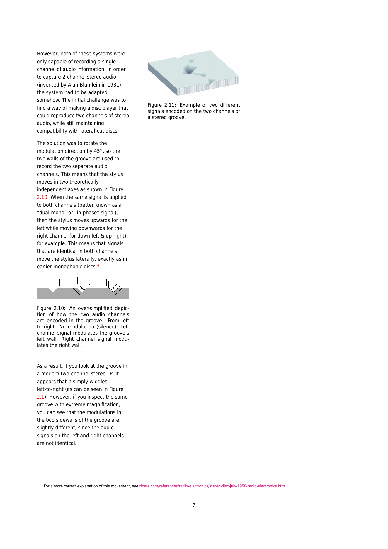
There are some disadvantages to this

system, such as the risk of the needle

slipping out of the groove when it is

too shallow, or suﬀering from

excessive wear if the groove is too

deep. In addition, any vertical variation

in the recording surface (such as a

cylinder that is not quite round, or

mechanical vibrations in the player

caused by footsteps in the room)

becomes translated into unwanted

noises upon playback.

Figure 2.7: An Edison cylinder player, on

display in the Struer Museum.

Figure 2.8: A closeup of the Edison

player. Notice that the needle is

mounted to move vertically, modulating

a me mb ran e located at the end of the

tonearm (the bent pipe).

Berliner’s Gram oph one used a diﬀerent

system, where the needle vibrated

sideways instead. This lateral cut

system produced a groove on the disc

with a constant depth, thus avoiding

some of the problems incurred by the

vertical cut recording system.

Figure 2.9: Example of an audio signal

encoded using a lateral cutting system.

see the Manual of Analogue Sound Restoration Techniques (2008), by Peter Copeland

Some 78 RPM discs use a vertical cutting system as well, including those made by Edison Disc Records a nd Pathé.

However, both of these systems were

only capable of recording a single

channel of audio information. In order

to capture 2-channel stereo audio

(invented by Alan Blumlein in 1931)

the system had to be adapted

somehow. The initial challenge was to

ﬁnd a way of making a disc player that

could reproduce two channels of stereo

audio, while still maintaining

compatibility with lateral-cut discs.

The solution was to rotate the

modulation direction by 45

◦

, so the

two walls of the groove are used to

record the two separate audio

channels. This means that the stylus

moves in two theoretically

independent axes as shown in Figure

2.10. When the same signal is applied

to both channels (better known as a

“dual-mono” or “in-phase” signal),

then the stylus moves upwards for the

left while moving downwards for the

right channel (or down-left & up-right),

for example. This means that signals

that are identical in both channels

move the stylus laterally, exactly as in

earlier monophonic discs.

Figure 2.10: An over-simpliﬁed depic-

tion of how the two audio channe ls

are encoded in the groove. From left

to right: No modulation (silence); Left

channel signal modulates the groove’s

left wall; Right channel signal modu-

lates the right wall.

As a result, if you look at the groove in

a modern two-channel stereo LP, it

appears that it simply wiggles

left-to-right (as can be seen in Figure

2.1). However, if you inspect the same

groove with extreme magniﬁcation,

you can see that the modulations in

the two sidewalls of the groove are

slightly diﬀerent, since the audio

signals on the left and right channels

are not identical.

Figure 2.11: Example of two diﬀerent

signals encode d on the two channe ls of

a stereo groove.

For a more correct explanation of this movement, s ee rfcafe.com/references/radio-electronics/stereo-disc-july-1958-radio-electronics.htm

The cartridge, stylus, and

tonearm

3.1 MMC: Micro Moving Cross

As mentioned above, when a wire is

moved through a magnetic ﬁeld, a

current is generated in it that is

proportional to the velocity of the

movement. In order to increase the

output, the wire can be wrapped into a

coil, eﬀectively lengthening the piece

of wire moving through the ﬁeld. Most

phono cartridges make use of this

behaviour by using the movement of

the stylus to either:

• move tiny magnets that are

placed near coils of wire (a

Moving Magnet or MM design )

• move tiny coils of wire that are

placed near very strong magnets

(a Moving Coil or MC design)

In either system, there is a relative

physical movement that is used to

generate the electrical signal from the

cartridge. There are advantages and

disadvantages associated with both of

these systems, however, they will not

be discussed here.

There is a third, less common design

called a Moving Iron (or

variable-reluctance

) system, which

can be thought of as a variant of the

Moving Magnet principle. In this

design, the magnet and the coils

remain stationary, and the stylus

moves a small piece of iron instead.

That iron is placed between the north

and south poles of the magnet so that,

when it moves, it modulates (or varies)

the magnetic ﬁeld. As the magnetic

ﬁeld modulates, it moves relative to

the coils, and an electrical signal is

generated. One of the ﬁrst examples of

this kind of pickup was the Weste rn

Electric 4A reproducer made in 1925.

Figure 3.1: Figures from Rørbaek Mad-

sen’s 196 3 patent for a Stereophonic

Transducer Cartridge.

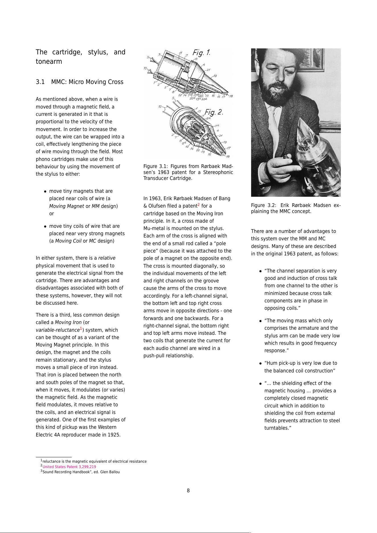
In 1963, Erik Rørbaek Madsen of Bang

& Olufsen ﬁled a patent

for a

cartridge based on the Moving Iron

principle. In it, a cross made of

Mu-metal is mounted on the stylus.

Each arm of the cross is aligned with

the end of a small rod called a “pole

piece” (because it was attached to the

pole of a magnet on the opposite end).

The cross is mounted diagonally, so

the individual movements of the left

and right channels on the groove

cause the arms of the cross to move

accordingly. For a left-channel signal,

the bottom left and top right cross

arms move in opposite directions - one

forwards and one backwards. For a

right-channel signal, the bottom right

and top left arms move instead. The

two coils that generate the current for

each audio channel are wired in a

push-pull relationship.

Figure 3.2: Erik Rørbaek Madsen ex-

plaining the MMC concept.

There are a number of advantages to

this system over the MM and MC

designs. Many of these are described

in the original 1963 patent, as follows:

• “The channel separation is very

good and induction of cross talk

from one channel to the other is

minimized because cross talk

components are in phase in

opposing coils.”

• “The moving mass which only

comprises the armature and the

stylus arm can be made very low

which results in good frequency

response.”

• “Hum pick-up is very low due to

the balanced coil construction”

• “... the shielding eﬀect of the

magnetic housing ... provides a

completely closed magnetic

circuit which in addition to

shielding the coil from external

ﬁelds prevents attraction to steel

turntables.”

reluctance is the magnetic equivalent of electrical resistance

United States Patent 3,299,219

Sound Recording Handbook”, ed. Glen Ballou

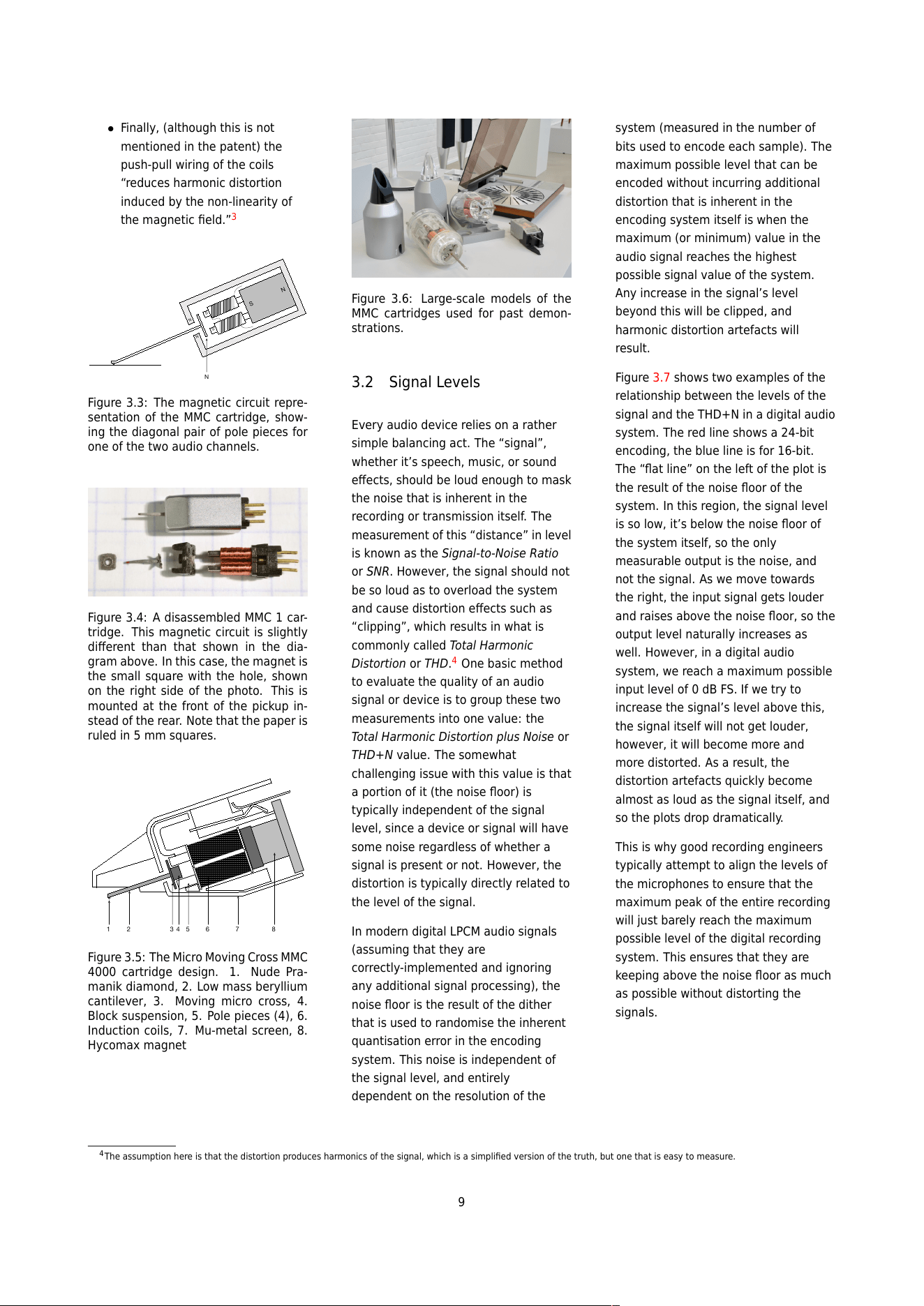
• Finally, (although this is not

mentioned in the patent) the

push-pull wiring of the coils

“reduces harmonic distortion

induced by the non-linearity of

the magnetic ﬁeld.”

Figure 3.3: The magnetic circuit repre-

sentation of the MMC cartridge, show-

ing the diagonal pair of pole pieces for

one of the two audio channels.

Figure 3.4: A disassembled MMC 1 car-

tridge. This magnetic circuit is slightly

diﬀerent than that shown in th e dia-

gram above. In this case, the magnet is

the small square with the hole, shown

on the right side of the photo. This is

mounted at the front of the pickup in-

stead of the rear. Note that the paper is

ruled in 5 mm squares.

1 2 3 4 5 6 7 8

Figure 3.5: The Micro Moving Cross MMC

4000 cartridge design. 1. Nude Pra-

manik diamond, 2. Low mass ber ylliu m

cantilever, 3. Moving micro cross, 4.

Block suspen sio n, 5. Pole pieces (4), 6.

Induction coils, 7. Mu-metal screen, 8.

Hycomax magnet

Figure 3.6: Large-scale models of the

MMC cartridges used for past demon-

strations.

3.2 Signal Levels

Every audio device relies on a rather

simple balancing act. The “signal”,

whether it’s speech, music, or sound

eﬀects, should be loud enough t o mask

the noise that is inherent in the

recording or transmission itself. The

measurement of this “distance” in level

is known as the Signal-to-Noise Ratio

or SNR. However, the signal should not

be so loud as to overload the system

and cause distortion eﬀects such as

“clipping”, which results in what is

commonly called Total Harmonic

Distortion or THD.

One basic method

to evaluate the quality of an audio

signal or device is to group these two

measurements into one value: the

Total Harmonic Distortion plus Noise or

THD+N value. The somewhat

challenging issue with this value is that

a portion of it (the noise ﬂoor) is

typically independent of the signal

level, since a device or signal will have

some noise regardless of whether a

signal is present or not. However, the

distortion is typically directly related to

the level of the signal.

In modern digital LPCM audio signals

(assuming that they are

correctly-implemented and ignorin g

any additional signal processing), the

noise ﬂoor is the result of the dither

that is used to randomise the inherent

quantisation error in the encoding

system. This noise is independent of

the signal level, and entirely

dependent on the resolution of the

system (measured in the number of

bits used to encode each sample). The

maximum possible level that can be

encoded without incurring additional

distortion that is inherent in the

encoding system itself is when the

maximum (or minimum) value in the

audio signal reaches the highest

possible signal value of the system.

Any increase in the signal’s level

beyond this will be clipped, and

harmonic distortion artefacts will

result.

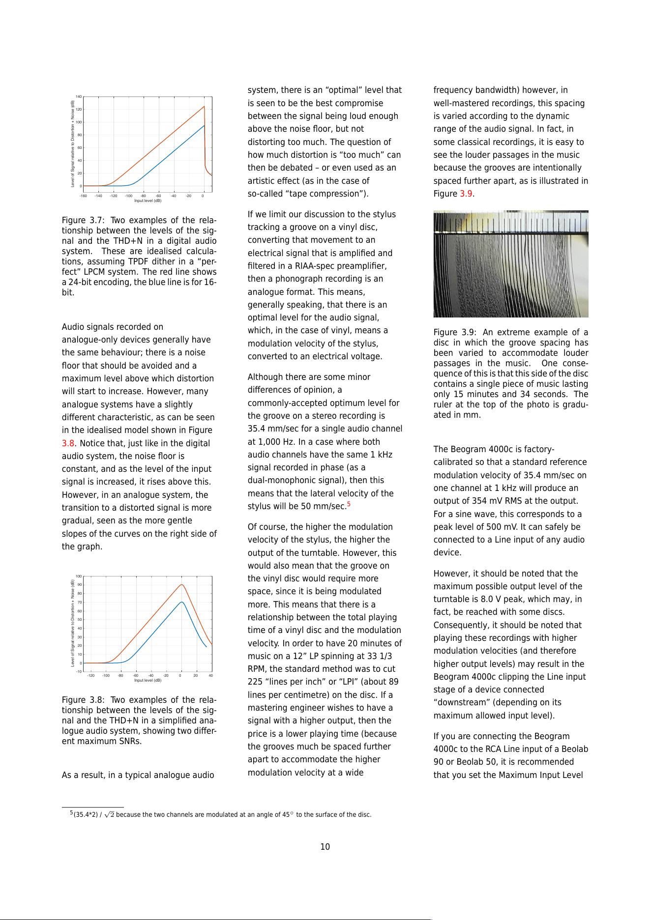
Figure 3.7 shows two examples of the

relationship between the levels of the

signal and the THD+N in a digita l audio

system. The red line shows a 24-bit

encoding, the blue line is for 16-bit.

The “ﬂat line” on the left of the plot is

the result of the noise ﬂoor of the

system. In this region, the signal level

is so low, it’s below the noise ﬂoor of

the system itself, so the only

measurable output is the noise, and

not the signal. As we move towards

the right, the input signal gets louder

and raises above the noise ﬂoor, so the

output level naturally increases as

well. However, in a digital audio

system, we reach a maximum possible

input level of 0 dB FS. If we try to

increase the signal’s level above this,

the signal itself will not get louder,

however, it will become more and

more distorted. As a result, the

distortion artefacts quickly become

almost as loud as the signal itself, and

so the plots drop dramatically.

This is why good recording engineers

typically attempt to align the levels of

the microphones to ensure that the

maximum peak of the entire recording

will just barely reach the maximum

possible level of the digital recording

system. This ensures that they are

keeping above the noise ﬂoor as much

as possible without distorting the

signals.

The assumption here is that the distortion produces harmonics of the signal, which is a simpliﬁed v er s ion o f t he truth, but one that is easy to measure.

-160 -140 -120 -100 -80 -60 -40 -20 0

Input level (dB)

100

120

140

Level of Signal relative to Distortion + Noise (dB)

Figure 3.7: Two examples of the rela-

tionship between the levels of the sig-

nal an d the THD+N in a digital audio

system. These are idealised calcula-

tions, as s um ing TPDF dither in a “per-

fect” LPCM system. The red line shows

a 24-bit encoding, the blue line is for 16-

bit.

Audio signals recorded on

analogue-only devices generally have

the same behaviour; there is a noise

ﬂoor that should be avoided and a

maximum level above which distortion

will start to increase. How e ve r, ma ny

analogue systems have a slightly

diﬀerent characteristic, as can be seen

in the idealised model shown in Figure

3.8. Notice that, just like in the digital

audio system, the noise ﬂoor is

constant, and as the level of the input

signal is increased, it rises above this.

However, in an analogue system, the

transition to a distorted signal is more

gradual, seen as the more gentle

slopes of the curves on the right side of

the graph.

-120 -100 -80 -60 -40 -20 0 20 40

Input level (dB)

-10

100

Level of Signal relative to Distortion + Noise (dB)

Figure 3.8: Two examples of the rela-

tionship between the levels of the sig-

nal and the THD+N in a simpliﬁed ana-

logue audio system, showing two diﬀer-

ent maximum SNRs.

As a result, in a typical analogue audio

system, there is an “optimal” level that

is seen to be the best compromise

between the signal being loud enough

above the noise ﬂoor, but not

distorting too much. The question of

how much distortion is “too much” can

then be debated – or even used as an

artistic eﬀect (as in the case of

so-called “tape compression”).

If we limit our discussion to the stylus

tracking a groove on a vinyl disc,

converting that movement to an

electrical signal that is ampliﬁed and

ﬁltered in a RIAA-spec preampliﬁer,

then a phonograph recording is an

analogue format. This means,

generally speaking, that there is an

optimal level for the audio signal,

which, in the case of vinyl, means a

modulation velocity of the stylus,

converted to an electrical voltage.

Although there are some minor

diﬀerences of opinion, a

commonly-accepted optimum level for

the groove on a stereo recording is

35.4 mm/sec for a single audio channel

at 1,000 Hz. In a case where both

audio channels have the same 1 kHz

signal recorded in phase (as a

dual-monophonic signal), then this

means that the lateral velocity of the

stylus will be 50 mm/sec.

Of course, the higher the modulation

velocity of the stylus, the higher the

output of the turntable. However, this

would also mean that the groove on

the vinyl disc would require more

space, since it is being modulated

more. This means that there is a

relationship between the total playing

time of a vinyl disc and the modulation

velocity. In order to have 20 minutes of

music on a 12” LP spinning at 33 1/3

RPM, the standard method was to cut

225 “lines per inch” or “LPI” (about 89

lines per centimetre) on the disc. If a

mastering engineer wishes to have a

signal with a higher output, then the

price is a lower playing time (because

the grooves much be spaced further

apart to accommodate the higher

modulation velocity at a wide

frequency bandwidth) however, in

well-mastered recordings, this spacing

is varied according to the dynamic

range of the audio signal. In fact, in

some classical recordings, it is easy to

see the louder passages in the music

because the grooves are intentionally

spaced further apart, as is illustrated in

Figure 3.9.

Figure 3.9: An extreme example of a

disc in which the groove spacing has

been varied to accommodate louder

passages in the mus ic . One conse-

quence of this is that this side of the disc

contains a single piece of music lasting

only 15 minutes and 34 seconds. The

ruler at the top of the photo is gradu-

ated in mm.

The Beogram 4000c is factory-

calibrated so that a standard reference

modulation velocity of 35.4 mm/sec on

one channel at 1 kHz will produce an

output of 354 mV RMS at the output.

For a sine wave, this corresponds to a

peak level of 500 mV. It can safely be

connected to a Line input of any audio

device.

However, it should be noted that the

maximum possible output level of the

turntable is 8.0 V peak, which may, in

fact, be reached with some discs.

Consequently, it should be noted that

playing these recordings with higher

modulation velocities (and therefore

higher output levels) may result in the

Beogram 4000c clipping the Line input

stage of a device connected

“downstream” (depending on its

maximum allowed input level).

If you are connecting the Beogram

4000c to the RCA Line input of a Be ola b

90 or Beolab 50, it is recommended

that you set the Maximum Input Level

(35.4*2) /

√

2 because the two channels are modulated at an angle of 45

◦

to the surface of the disc.

of that input on the loudspeaker to 4.0

V RMS (which corresponds to 5.7 V

peak) or 6.5 V RMS (9.2 V peak) using

its Input Setup menu. This will ensure

that you maintain adequate headroom

for playback.

A large part of the performance of a

turntable is dependent on the physical

contact between the surface of the

vinyl and the tip of the stylus. In

general terms, as we’ve already seen,

there is a groove with two walls that

vary in height, almost independently

and the tip of the stylus traces that

movement accordingly. However, it is

necessary to get down to the

microscopic level to consider this

behaviour in more detail.

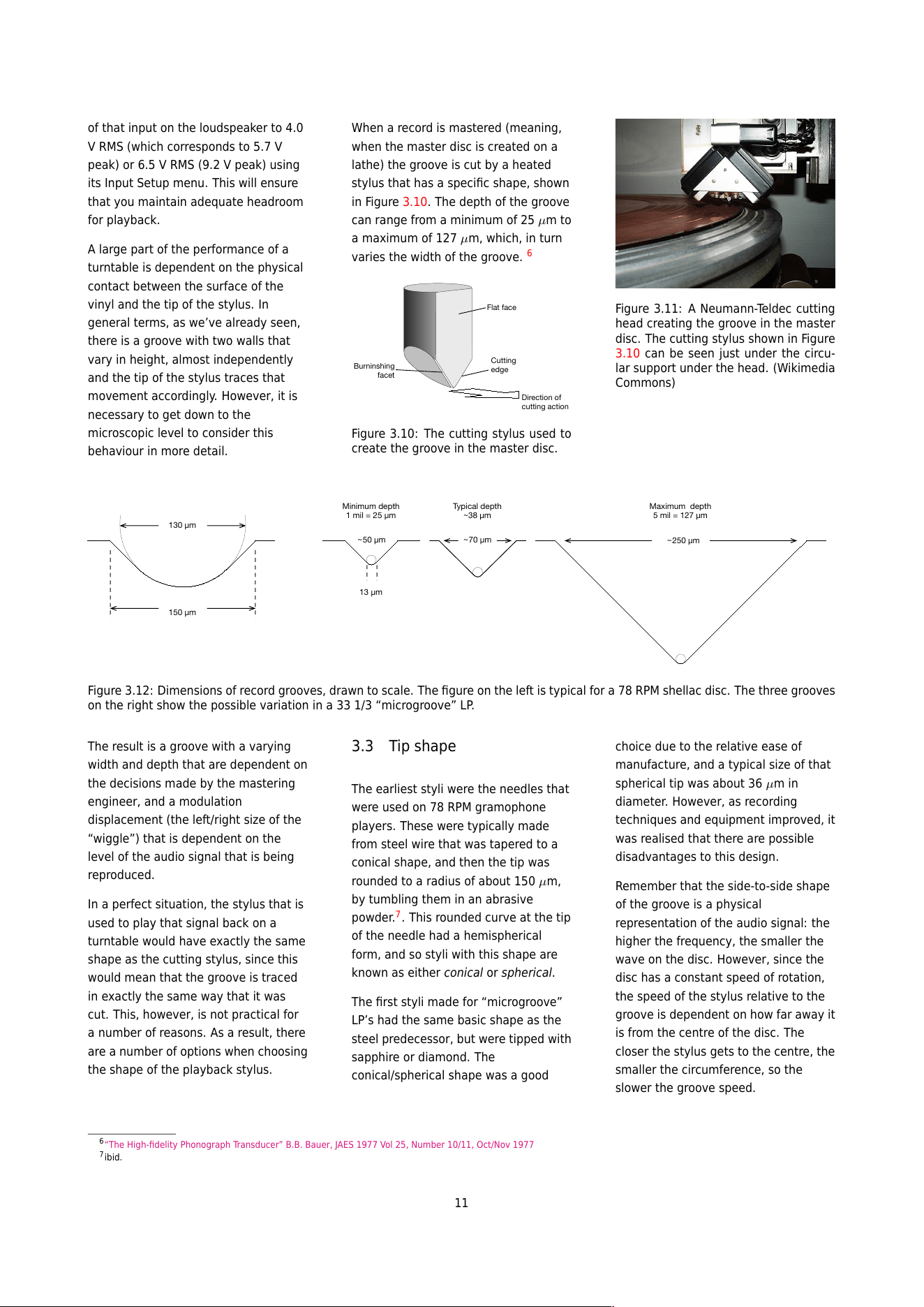
When a record is mastered (meaning,

when the master disc is created on a

lathe) the groove is cut by a heated

stylus that has a speciﬁc shape, shown

in Figure 3.10. The depth of the groove

can range from a minimum of 25 µm to

a maximum of 127 µm, which, in turn

varies the width of the groove.

Flat face

Burninshing!

facet

Cutting!

edge

Direction of!

cutting action

Figure 3.10: The cutting stylus used to

create the groove in the master disc.

Figure 3.11: A Neumann-Teldec cutting

head creating the groove in the master

disc. The cutting stylus shown in Figure

3.10 can be seen just under the circu-

lar support under the head. (Wikimedia

Commons)

150 µm

130 µm

13 µm

Minimum depth!

1 mil = 25 µm

Typical depth

~38 µm

Maximum depth!

5 mil = 127 µm

~ 70 µm

~ 250 µm

~ 50 µm

Figure 3.12: Dimensions of record grooves, dra wn to scale. The ﬁgure on the left is typical for a 78 RPM shellac disc. The three grooves

on the right show the possible variation in a 33 1/3 “microgroove” LP.

The result is a groove with a varying

width and depth that are dependent on

the decisions made by the mastering

engineer, and a modulation

displacement (the left/right size of the

“wiggle”) that is dependent on the

level of the audio signal that is being

reproduced.

In a perfect situation, the stylus that is

used to play that signal back on a

turntable would have exactly the same

shape as the cutting stylus, since this

would mean that the groove is traced

in exactly the same way that it was

cut. This, however, is not practical for

a number of reasons. As a result, there

are a number of options when choosing

the shape of the playback stylus.

3.3 Tip shape

The earliest styli were the needles that

were used on 78 RPM gramophone

players. These were typically made

from steel wire that was tapered to a

conical shape, and then the tip was

rounded to a radius of about 150 µm,

by tumbling them in an abrasive

powder.

. This rounded curve at the tip

of the needle had a hemispherical

form, and so styli with this shape are

known as either conical or spherical.

The ﬁrst styli made for “microgroove”

LP’s had the same basic shape as the

steel predecessor, but were tipped with

sapphire or diamond. The

conical/spherical shape was a good

choice due to the relative ease of

manufacture, and a typical size of that

spherical tip was about 36 µm in

diameter. However, as recording

techniques and e quip me nt improved, it

was realised that there are possible

disadvantages to this design.

Remember that the side-to-side shape

of the groove is a physical

representation of the audio signal: the

higher the frequency, the smaller the

wave on the disc. However, since the

disc has a constant speed of rotation,

the speed of the stylus relative to the

groove is dependent on how far away it

is from the centre of the disc. The

closer the stylus gets to the centre, the

smaller the circumference, so the

slower the groove speed.

“The High-ﬁdelity Phonograph Transducer” B. B. Bauer, JAES 1977 Vol 25, Number 10/11, Oct/Nov 1977

ibid.

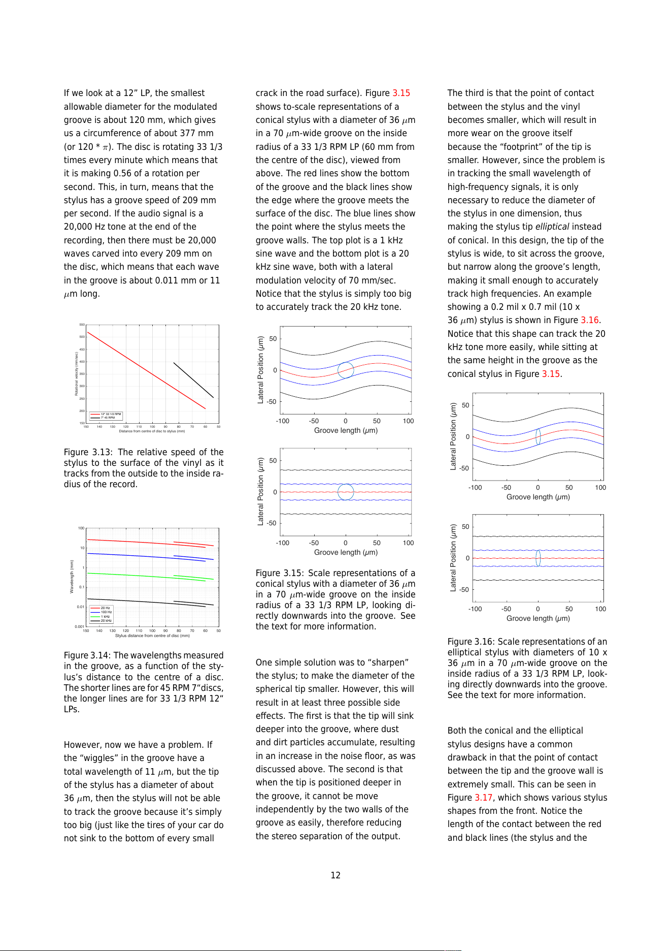
If we look at a 12” LP, the smallest

allowable diameter for the modulated

groove is about 120 mm, which gives

us a circumference of about 377 mm

(or 120 * π). The disc is rotating 33 1/3

times every minute which means that

it is making 0.56 of a rotation per

second. This, in turn, means that the

stylus has a groove speed of 209 mm

per second. If the audio signal is a

20,000 Hz tone at the end of the

recording, then there must be 20,000

waves carved into every 209 mm on

the disc, which means that each wave

in the groove is about 0.011 mm or 11

µm long.

5060708090100110120130140150

Distance from centre of disc to stylus (mm)

150

200

250

300

350

400

450

500

550

Rotational velocity (mm/sec)

12" 33 1/3 RPM

7" 45 RPM

Figure 3.13: The relative speed of the

stylus to the surfac e of the vinyl as it

tracks from the out s ide to the inside ra-

dius of the record.

5060708090100110120130140150

Stylus distance from centre of disc (mm)

0.001

0.01

0.1

100

Wavelength (mm)

20 Hz

100 Hz

1 kHz

20 kHz

Figure 3.14: The wavelengths me as ured

in the gro ove , as a function of the sty-

lus’s distance to the centre of a disc.

The shorter lines are for 45 RPM 7“discs,

the longer lines are for 33 1/3 RPM 12“

LPs.

However, now we have a problem. If

the “wiggles” in the groove have a

total wavelength of 11 µm, but the tip

of the stylus has a diameter of about

36 µm, then the stylus will not be able

to track the groove because it’s simply

too big (just like the tires of your car do

not sink to the bottom of every small

crack in the road surface). Figure 3.15

shows to-scale representations of a

conical stylus with a diameter of 36 µm

in a 70 µm-wide groove on the inside

radius of a 33 1/3 RPM LP (60 mm from

the centre of the disc), viewed from

above. The red lines show the bottom

of the groove and the black lines show

the edge where the groove meets the

surface of the disc. The blue lines show

the point where the stylus meets the

groove walls. The top plot is a 1 kHz

sine wave and the bottom plot is a 20

kHz sine wave, both with a lateral

modulation velocity of 70 mm/sec.

Notice that the stylus is simply too big

to accurately track the 20 kHz tone.

-100 -50 0 50 100

Groove length (µm)

-50

Lateral Position (µm)

-100 -50 0 50 100

Groove length (µm)

-50

Lateral Position (µm)

Figure 3.15: Scale representations of a

conical stylus with a diameter of 36 µm

in a 70 µm-wide groove on the inside

radius of a 33 1/3 RPM LP, looking di-

rectly downwards into the groove. See

the text for more information.

One simple solution was to “sharpen”

the stylus; to make the diameter of the

spherical tip smaller. However, this will

result in at least three possible side

eﬀects. The ﬁrst is that the tip will sink

deeper into the groove, where dust

and dirt particles accumulate, resulting

in an increase in the noise ﬂoor, as was

discussed above. The second is that

when the tip is positioned deeper in

the groove, it cannot be move

independently by the two walls of the

groove as easily, therefore reducing

the stereo separation of the output.

The third is that the point of contact

between the stylus and the vinyl

becomes smaller, which will result in

more wear on the groove itself

because the “footprint” of the tip is

smaller. However, since the problem is

in tracking the small wavelength of

high-frequency signals, it is only

necessary to reduce the diameter of

the stylus in one dimension, thus

making the stylus tip elliptical instead

of conical. In this design, the tip of the

stylus is wide, to sit across the groove,

but narrow along the groove’s length,

making it small enough to accurately

track high frequencies. An example

showing a 0.2 mil x 0.7 mil (10 x

36 µm) stylus is shown in Figure 3.16.

Notice that this shape can track the 20

kHz tone more easily, while sitting at

the same height in the groove as the

conical stylus in Figure 3.15.

-100 -50 0 50 100

Groove length (µm)

-50

Lateral Position (µm)

-100 -50 0 50 100

Groove length (µm)

-50

Lateral Position (µm)

Figure 3.16: Scale representations of an

elliptical stylus with diameters of 10 x

36 µm in a 70 µm-wide groove on the

inside radius of a 33 1/3 RPM L P, look-

ing directly downwards into the groove.

See the text for more information.

Both the conical and the elliptical

stylus designs have a common

drawback in that the point of contact

between the tip and the groove wall is

extremely small. This can be seen in

Figure 3.17, which shows various stylus

shapes from the front. Notice the

length of the contact between the red

and black lines (the stylus and the

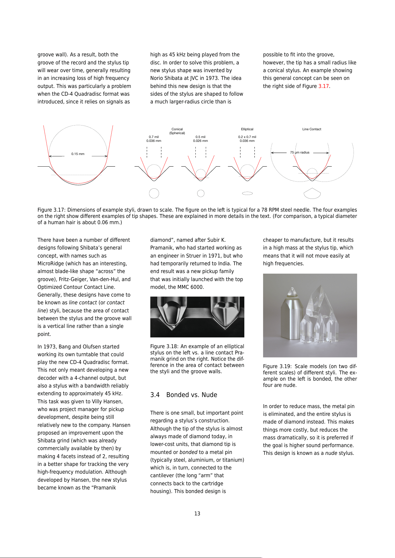
groove wall). As a result, both the

groove of the record and the stylus tip

will wear over time, generally resulting

in an increasing loss of high frequency

output. This was particularly a problem

when the CD-4 Quadradisc format was

introduced, since it relies on signals as

high as 45 kHz being played from the

disc. In order to solve this problem, a

new stylus shape was invented by

Norio Shibata at JVC in 1973. The idea

behind this new design is that the

sides of the stylus are shaped to follow

a much larger-radius circle than is

possible to ﬁt into the groove,

however, the tip has a small radius like

a conical stylus. An example showing

this general concept can be seen on

the right side of Figure 3.17.

0.036 mm

0.7 mil 0.5 mil

Conical!

(Spherical)

Elliptical!

0.2 x 0.7 mil

0.026 mm 0.036 mm

75 µm radius

0.15 mm

Line Contact!

Figure 3.17: Dimensions of example styli, drawn to scale. The ﬁgure on the left is typical for a 78 RPM s te el needle. The four examples

on the right show diﬀerent examples of tip shapes. These are explained in more details in the text. (For comparison, a typical diameter

of a human hair is about 0.06 mm.)

There have been a number of diﬀerent

designs following Shibata’s general

concept, with names such as

MicroRidge (which has an interesting,

almost blade-like shape “across” the

groove), Fritz-Geiger, Van-den-Hul, and

Optimized Contour Contact Line.

Generally, these designs have come to

be known as line contact (o r cont ac t

line) styli, because the area of contact

between the stylus and the groove wall

is a vertical line rather than a single

point.

In 1973, Bang and Olufsen started

working its own turntable that could

play the new CD-4 Quadradisc format.

This not only meant developing a new

decoder with a 4-channel output, but

also a stylus with a bandwidth reliably

extending to approximately 45 kHz.

This task was given to Villy Hansen,

who was project manager for pickup

development, despite being still

relatively new to the company. Hansen

proposed an improvement upon the

Shibata grind (which was already

commercially available by then) by

making 4 facets instead of 2, resulting

in a better shape for tracking the very

high-frequency modulation. Although

developed by Hansen, the new stylus

became known as the “Pramanik

diamond”, named after Subir K.

Pramanik, who had started working as

an engineer in Struer in 1971, but who

had temporarily returned to India. The

end result was a new pickup family

that was initially launched with the top

model, the MMC 6000.

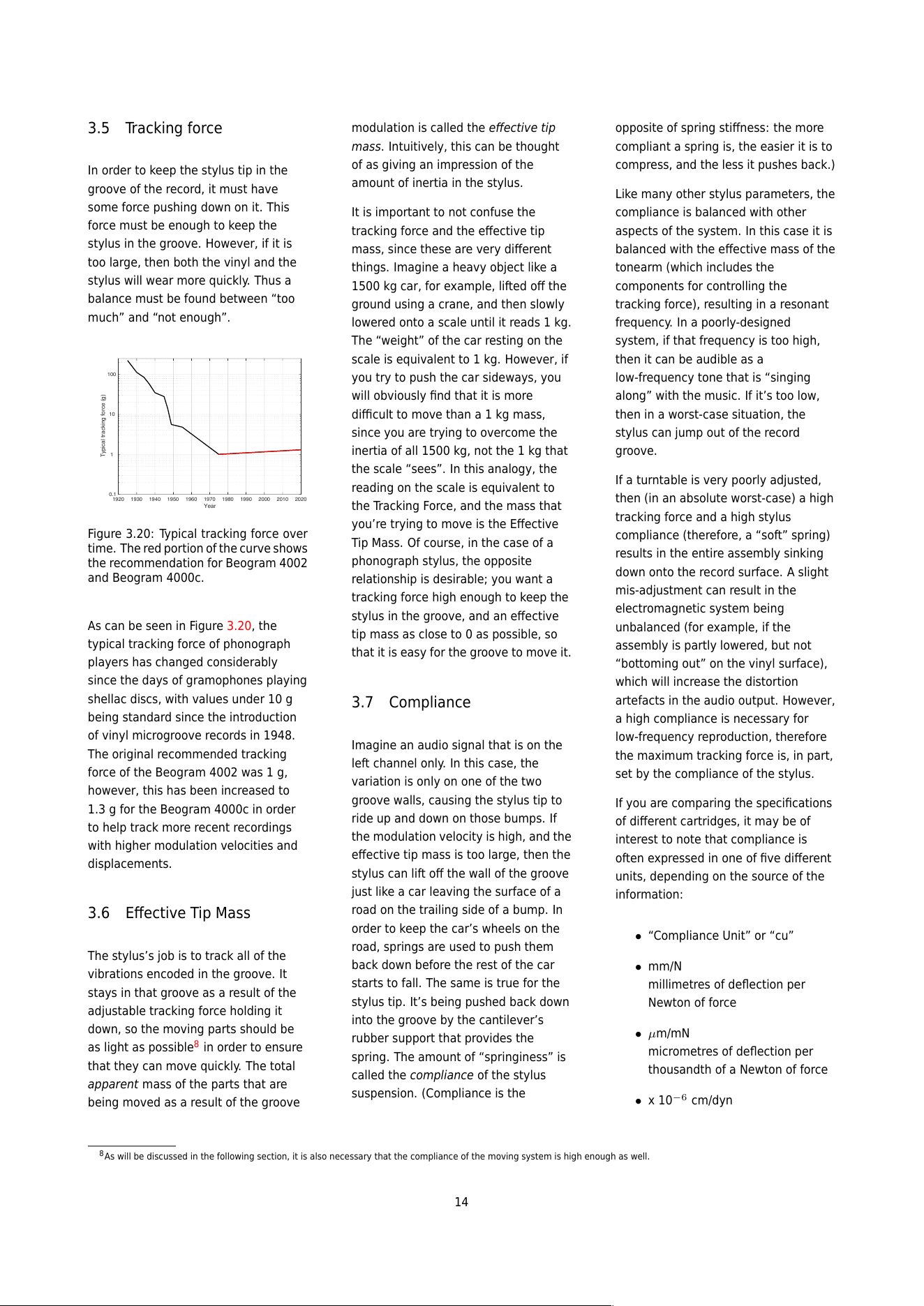
Figure 3.18: An example of an elliptical

stylus on the left vs. a line contact Pra-

manik grind on the right. Notice the dif-

ference in the area of contact between

the styli and the groove walls.

3.4 Bonded vs. Nude

There is one small, but important point

regarding a stylus’s construction.

Although the tip of the stylus is almost

always made of diamond today, in

lower-cost units, that diamond tip is

mounted or bonded to a metal pin

(typically steel, aluminium, or titanium)

which is, in turn, connected to the

cantilever (the long “arm” that

connects back to the cartridge

housing). This bonded design is

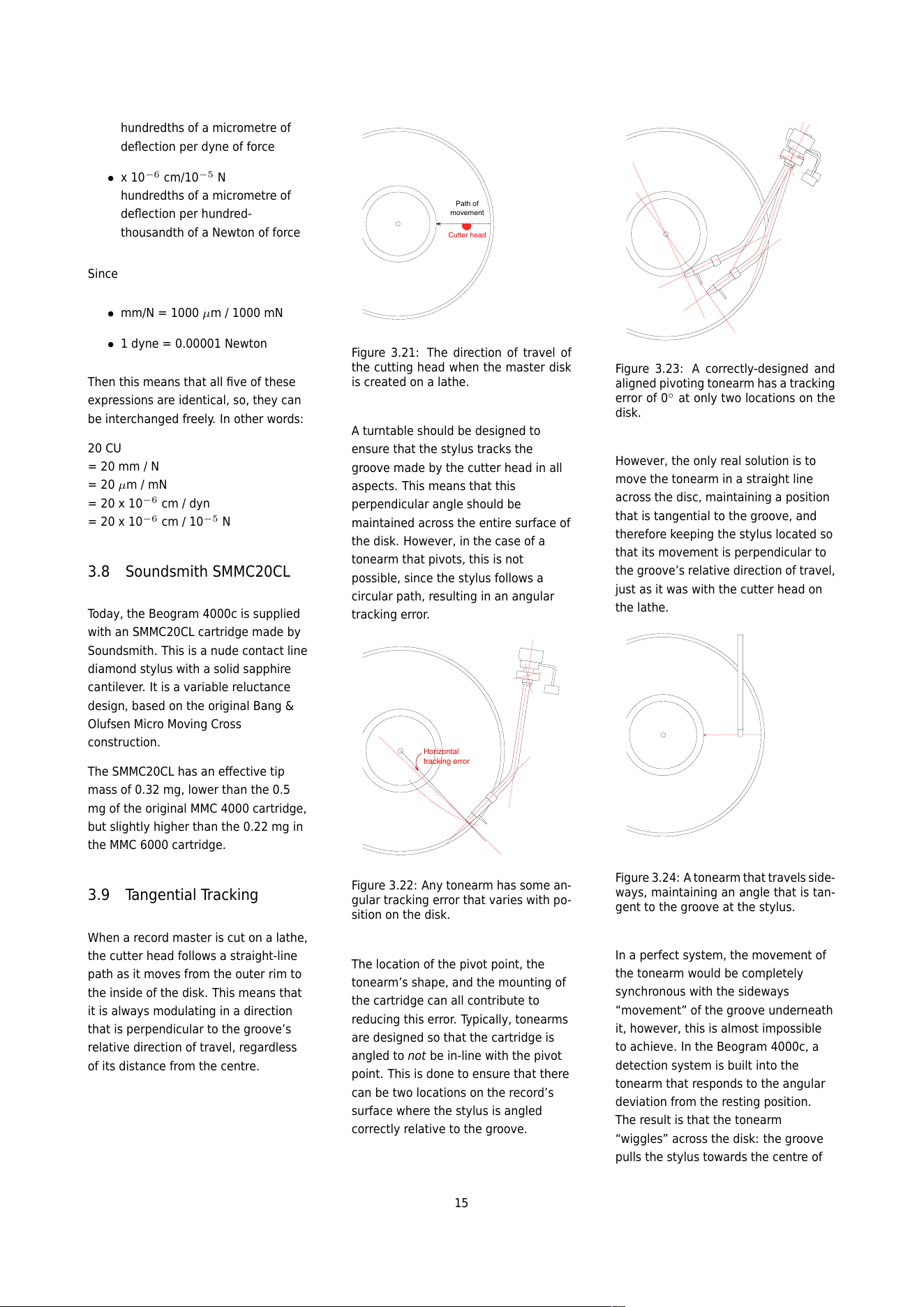
cheaper to manufacture, but it results

in a high mass at the stylus tip, which

means that it will not move easily at

high frequencies.

Figure 3.19: Scale models (on two dif-

ferent scales) of diﬀerent styli. The ex-

ample on the left is bonded, the other

four are nude.

In order to reduce mass, the metal pin

is eliminated, and the entire stylus is

made of diamond instead. This makes

things more costly, but reduces the

mass dramatically, so it is preferred if

the goal is higher sound performance.

This design is known as a nude stylus.

3.5 Tracking force

In order to keep the stylus tip in the

groove of the record, it must have

some force pushing down on it. This

force must be enough to keep the

stylus in the groove. Howev er , if it is

too large, then both the vinyl and the

stylus will wear more quickly. Thus a

balance must be found between “too

much” and “not enough”.

1920 1930 1940 1950 1960 1970 1980 1990 2000 2010 2020

Year

0.1

100

Typical tracking force (g)

Figure 3.20: Typical tracking force over

time. The red portion of the curve shows

the recommendation for Beogram 4002

and Beogram 4000c.

As can be seen in Figure 3.20, the

typical tracking force of phonograph

players has changed considerably

since the days of gramophones playing

shellac discs, with values under 10 g

being standard since the introduction

of vinyl microgroove records in 1948.

The original recommended tracking

force of the Beogram 4002 was 1 g,

however, this has been increased to

1.3 g for the Beogram 4000c in order

to help track more recent recordings

with higher modulation velocities and

displacements.

3.6 Eﬀective Tip Mass

The stylus’s job is to track all of the

vibrations encoded in the groove. It

stays in that groove as a result of the

adjustable tracking force holding it

down, so the moving parts should be

as light as possible

in order to ensure

that they can move quickly. The total

apparent mas s of the par ts th at are

being moved as a result of the groove

modulation is called the eﬀective tip

mass. Intuitively, this can be thought

of as giving an impression of the

amount of inertia in the stylus.

It is important to not confuse the

tracking force and the eﬀective tip

mass, since these are very diﬀerent

things. Imagine a heavy object like a

1500 kg car, for example, lifted oﬀ the

ground using a crane, and then slowly

lowered onto a scale until it reads 1 kg.

The “weight” of the car resting on the

scale is equivalent to 1 kg. However, if

you try to push the car sideways, you

will obviously ﬁnd that it is more

diﬃcult to move than a 1 kg mass,

since you are trying to overcome the

inertia of all 1500 kg, not the 1 kg that

the scale “sees”. In this analogy, the

reading on the scale is equivalent to

the Tracking Force, and the mass that

you’re trying to move is the Eﬀective

Tip Mass. Of course, in the case of a

phonograph stylus, the opposite

relationship is desirable; you want a

tracking force high enough to keep the

stylus in the groove, and an eﬀective

tip mass as close to 0 as possible, so

that it is easy for the groove to move it.

3.7 Compliance

Imagine an audio signal that is on the

left channel only. In this case, the

variation is only on one of the two

groove walls, causing the stylus tip to

ride up and down on those bumps. If

the modulation velocity is high, and the

eﬀective tip mass is too large, then the

stylus can lift oﬀ the wall of the groove

just like a car leaving the surface of a

road on the trailing side of a bump. In

order to keep the car’s wheels on the

road, springs are used to push them

back down before the rest of the car

starts to fall. The same is true for the

stylus tip. It’s being pushed back down

into the groove by the cantilever’s

rubber support that provides the

spring. The amount of “springiness” is

called the compliance of the stylus

suspension. (Compliance is the

opposite of spring stiﬀness: the more

compliant a spring is, the easier it is to

compress, and the less it pushes back.)

Like many other stylus parameters, the

compliance is balanced with other

aspects of the system. In this case it is

balanced w ith the eﬀective mass of the

tonearm (which includes the

components for controlling the

tracking force), resulting in a resonant

frequency. In a poorly-designed

system, if that frequency is too high,

then it can be audible as a

low-frequency tone that is “singing

along” with the music. If it’s too low,

then in a worst-case situation, the

stylus can jump out of the record

groove.

If a turntable is very poorly adjusted,

then (in an absolute worst-case) a high

tracking force and a high stylus

compliance (therefore, a “soft” spring)

results in the entire assembly sinking

down onto the record surface. A slight

mis-adjustment can result in the

electromagnetic system being

unbalanced (for example, if the

assembly is partly lowered, but not

“bottoming out” on the vinyl surface),

which will increase the distortion

artefacts in the audio output. However,

a high compliance is necessary for

low-frequency reproduction, therefore

the maximum tracking force is, in part,

set by the compliance of the stylus.

If you are comparing the speciﬁcations

of diﬀerent cartridges, it may be of

interest to note that compliance is

often expressed in one of ﬁve diﬀerent

units, depending on the source of the

information:

• “Compliance Unit” or “cu”

• mm/N

millimetres of deﬂection per

Newton of force

• µm/mN

micrometres of deﬂection per

thousandth of a Newton of force

• x 10

−6

cm/dyn

As will be discussed in the following section, it is also necessary that the compliance of the moving system is high enough as well.

hundredths of a micrometre of

deﬂection per dyne of force

• x 10

−6

cm/10

−5

hundredths of a micrometre of

deﬂection per hundred-

thousandth of a Newton of force

Since

• mm/N = 1000 µm / 1000 mN

• 1 dyne = 0.00001 Newton

Then this means that all ﬁve of these

expressions are identical, so, they can

be interchanged freely. In other words:

20 CU

= 20 mm / N

= 20 µm / mN

= 20 x 10

−6

cm / dyn

= 20 x 10

−6

cm / 10

−5

3.8 Soundsmith SMMC20CL

Today, the Beogram 4000c is supplied

with an SMMC20CL cartridge made by

Soundsmith. This is a nude contact line

diamond stylus with a solid sapphire

cantilever. It is a variable reluctance

design, based on the original Bang &

Olufsen Micro Moving Cross

construction.

The SMMC20CL has an eﬀective tip

mass of 0.32 mg, lower than the 0.5

mg of the original MMC 4000 cartridge,

but slightly higher than the 0.22 mg in

the MMC 6000 cartridge.

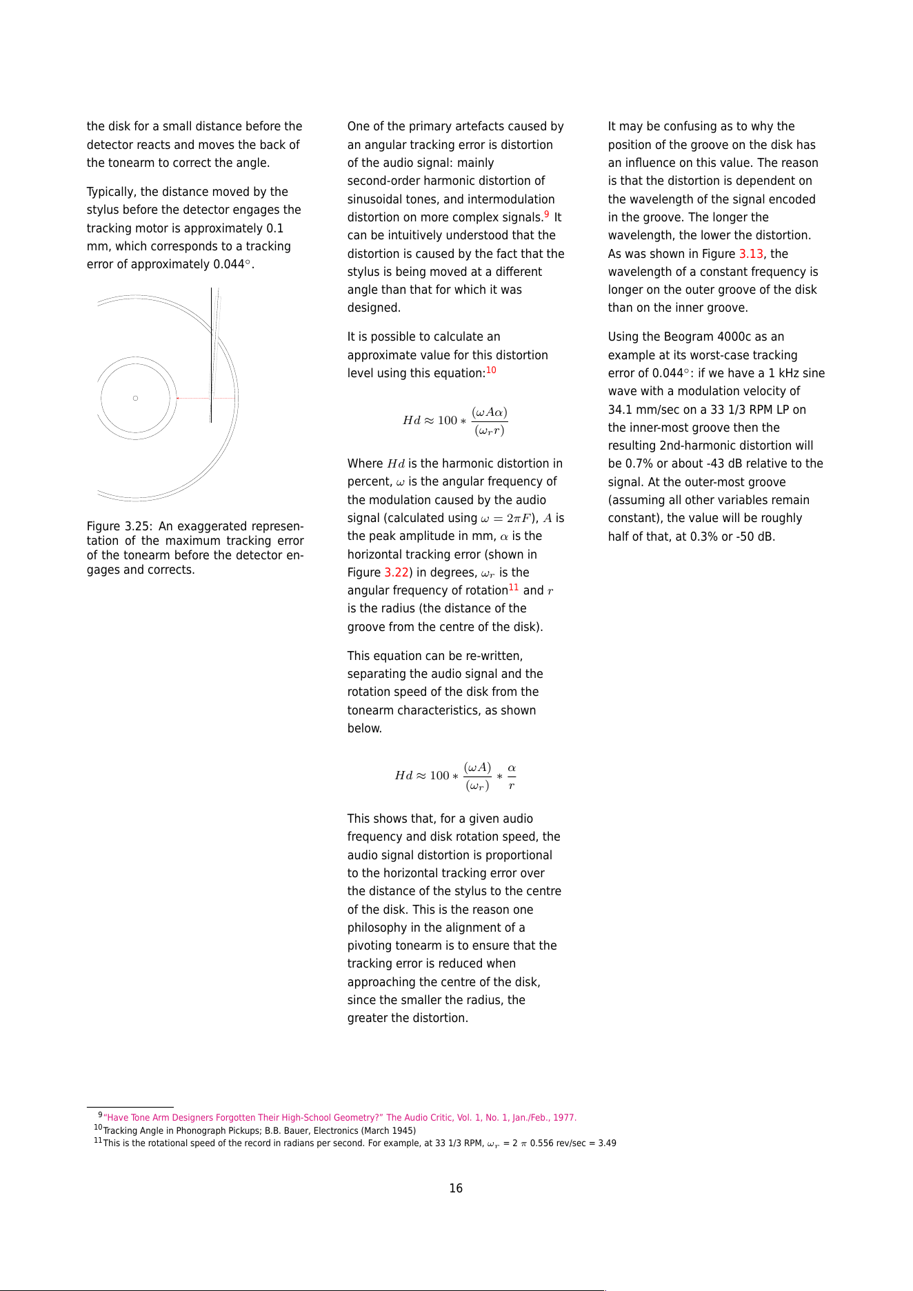
3.9 Tangential Tracking

When a record master is cut on a lathe,

the cutter head follows a straight-line

path as it moves from the outer rim to

the inside of the disk. This means that

it is always modulating in a direction

that is perpendicular to the groove’s

relative direction of travel, regardless

of its distance from the centre.

Cutter head

Path of

movement

Figure 3.21: The direction of travel of

the cutting head when the master disk

is created on a lathe.

A turntable should be designed to

ensure that the stylus tracks the

groove made by the cutter head in all

aspects. This means that this

perpendicular angle should be

maintained across the entire surface of

the disk. However, in the case of a

tonearm that pivots, this is not

possible, since the stylus follows a

circular path, resulting in an angular

tracking error.

Horizontal

tracking error

Figure 3.22: Any tonearm has some an-

gular tracking error that varies with po-

sition on the disk.

The location of the pivot point, the

tonearm’s shape, and the mounting of

the cartridge can all contribute to

reducing this error. Typically, tonearms

are designed so that the cartridge is

angled to not be in-line with the pivot

point. This is done to ensure that there

can be two locations on the record’s

surface where the stylus is angled

correctly relative to the groove.

Figure 3.23: A correctly-designed and

aligned pivoting tonearm has a tracking

error of 0

◦

at only two locations on the

disk.

However, the only real solution is to

move the tonearm in a straight line

across the disc, maintaining a position

that is tangential to the groove, and

therefore keeping the stylus located so

that its movement is perpendicular to

the groove’s relative direction of travel,

just as it was with the cutter head on

the lathe.

Figure 3.24: A tonearm that travels side-

ways, maintaining an angle that is tan-

gent to the groove at the stylus.

In a perfect system, the movement of

the tonearm would be completely

synchronous with the sideways

“movement” of the groove underneath

it, however, this is almost impossible

to achieve. In the Beogram 4000c, a

detection system is built into the

tonearm that responds to the angular

deviation from the resting position.

The result is that the tonearm

“wiggles” across the disk: the groove

pulls the stylus towards the centre of

the disk for a small distance before the

detector reacts and moves the back of

the tonearm to correct the angle.

Typically, the dist anc e mov ed by the

stylus before the detector engages the

tracking motor is approximate ly 0.1

mm, which corresponds to a tracking

error of approximate ly 0.04 4

◦

Figure 3.25: An exaggerated represen-

tation of the maximum tracking error

of the tonearm before the detector en-

gages and corrects.

One of the primary artefacts caused by

an angular tracking error is distortion

of the audio signal: mainly

second-order harmonic distortion of

sinusoidal tones, and intermodulation

distortion on more complex signals.

can be intuitively understood that the

distortion is c au se d by the fact that the

stylus is being moved at a diﬀerent

angle than that for which it was

designed.

It is possible to calculate an

approximate value for this distort ion

level using this equation:

Hd ≈ 100 ∗

(ωAα)

(ω

Where Hd is the harmonic distortion in

percent, ω is the angular frequency of

the modulation caused by the audio

signal (calculated using ω = 2πF ), A is

the peak amplitude in mm, α is the

horizontal tracking error (shown in

Figure 3.22) in degrees, ω

is the

angular frequency of rotation

and r

is the radius (the distance of the

groove from the centre of the disk).

This equation can be re-written,

separating the audio signal and the

rotation speed of the disk from the

tonearm characteristics, as shown

below.

Hd ≈ 100 ∗

(ωA)

(ω

)

∗

This shows that, for a given audio

frequency and disk rotation speed, the

audio signal distortion is proportional

to the horizontal tracking error over

the distance of the stylus to the centre

of the disk. This is the reason one

philosophy in the alignment of a

pivoting tonearm is to ensure that the

tracking error is reduced when

approaching the centre of the disk,

since the smaller the radius, the

greater the distortion.

It may be confusing as to why the

position of the groove on the disk has

an inﬂuence on this value. The reason

is that the distortion is dependent on

the wavelength of the signal encoded

in the groove. The longer the

wavelength, the lower the distortion.

As was shown in Figure 3.13, the

wavelength of a constant frequency is

longer on the outer groove of the disk

than on the inner groove.

Using the Beogram 4000c as an

example at its worst-case tracking

error of 0.044

◦

: if we have a 1 kHz sine

wave with a modulation velocity of

34.1 mm/sec on a 33 1/3 RPM LP on

the inner-most groove then the

resulting 2nd-harmonic distortion will

be 0.7% or about -43 dB relative to the

signal. At the outer-most groove

(assuming all other variables remain

constant), the value will be roughly

half of that, at 0.3% or -50 dB.

“Have Tone Arm Designers Forgotten Their High-School Geometry?” The Audio Critic, Vol. 1, No. 1, Jan./Feb., 1977.

Tracking Angle in Phonograph Pickups; B.B. Bauer, Electronics (March 1945)

This is the rotational speed of the record in radians per second. For example, at 33 1/3 RPM, ω

= 2 π 0.556 rev/sec = 3.49

Audio Speciﬁcations

4.0.1 Magnitude Response

The magnitude response

of any audio

device is a measure of how much its

output level deviates from the

expected level at diﬀerent frequencies.

In a turntable, this can be measured in

diﬀerent ways.

In the case of the Beogram 4000c, the

magnitude response is measured from

a standard test disc with a sine wave

sweep ranging from at least 20 Hz to at

least 20 kHz. The output level of this

signal is recorded at the output of the

device, and the level is analysed to

determine how much it diﬀers from the

expected output. Consequently, the

measurement includes all components

in the audio path from the stylus tip,

through the RIAA preampliﬁer, to the

line-level outputs.

4.0.2 Rumble

In theory, an audio playback device

only outputs the audio signal that is on

the recording without any extra

contributions. In practice, however,

every audio device adds signals to the

output for various reasons. As was

discussed above, in the speciﬁc case of

a turntable, the audio signal is initially

generated by very small movements of

the stylus in the record groove.

Therefore, in order for it to work at all,

the system must be sensitive to very

small movements in general. This

means that any additional movement

can (and probably will) be converted to

an audio signal that is added to the

recording.

This unwanted extraneous movement,

and therefore signal, is usually the

result of very low-frequency vibrations

that come from various sources. These

can include things like mechanical

vibrations of the entire turntable

transmitted through the table from the

ﬂoor, vibrations in the system caused

by the motor or imbalances in the

moving parts, warped discs which

cause a vertical movement of the

stylus, and so on. These low-frequency

signals are grouped together under the

heading of rumble.

A rumble measurement is performed

by playing a disc that has no signal on

it, and measuring the output signal’s

level. However, that output signal is

ﬁrst ﬁltered

to ensure that the level

detection is not inﬂuenced by

higher-frequency problems that may

exist.

If the standard being used for the

rumble measurement is the DIN 45 539

speciﬁcation, then the resulting value

is stated as the level diﬀerence

between the measured ﬁltered noise

and the standard output level,

equivalent to the output when playing

a 1 kHz tone with a lateral modulation

velocity of 70.7 mm/sec. In other

words, it states how much quieter the

rumble is than a relatively loud audio

signal.

4.0.3 Rotational speed

Every recording / playback system,

whether for audio or for video signals,

is based on the fundamental principle

that the recording and the playback

happen at the same rate. For example,

a ﬁlm that was recorded at 24 frames

(or photos) per second (FPS) must also

be played at 24 FPS to avoid objects

and persons moving too slowly or too

quickly. It’s also necessary that neither

the recording nor the playback speed

changes over time.

A phonographic LP is mastered with

the intention that it will be played back

at a rotational speed of 33 1/3 RPM

(Revolutions Per Minute) or 45 RPM,

depending on the disc. (These

correspond to 1 revolution either every

1.8 seconds or every 1 1/3 seconds

respectively.) We assume that the

rotational speed of the lathe that was

used to cut the master was both very

accurate and very stable. Although it is

the job of the turntable to duplicate

this ac cu ra cy and stability as closely as

possible, measurable errors occur for a

number of reasons, both mechanical

and electrical. When these errors are

measured using especially-created

audio signals like pure sine tones, the

results are ﬁltered and analyzed to

give an impression of how audible they

are when listening to music. However,

a problem arises in that a simple

speciﬁcation (such as a single number

for “Wow and Flutter”, for example)

can only be correctly interpreted with

the knowledge of how the value is

produced.

Accuracy

The ﬁrst issue is the simple one of

accuracy: is the turntable rotating the

disc at the correct average speed? In

the Beogram 4000c, this speed is

governed by a tachometer built into

the drive motor, that (like on almost all

turntables) can be adjusted by the user

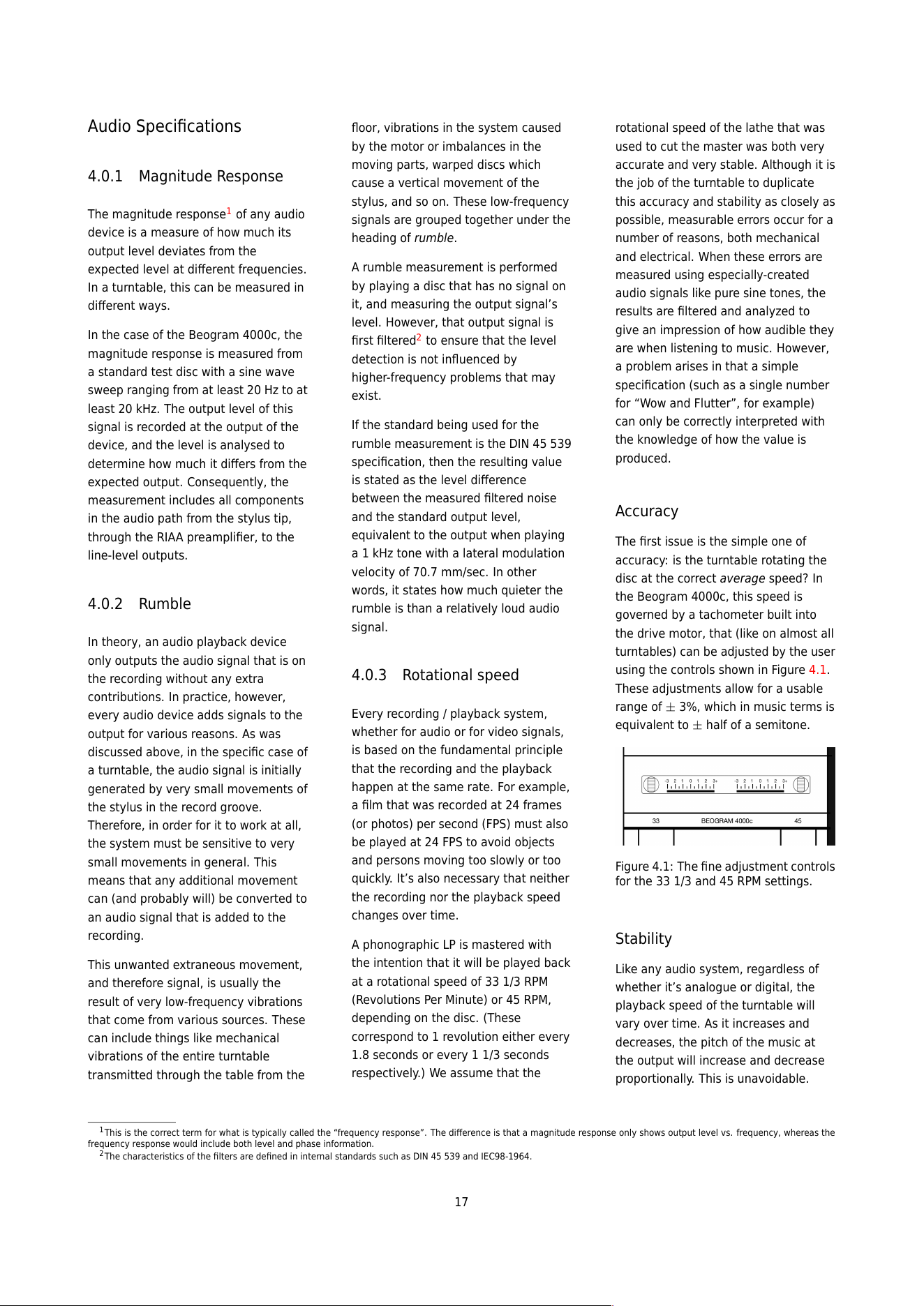
using the controls shown in Figure 4.1.

These adjustments allow for a usable

range of ± 3%, which in music terms is

equivalent to ± half of a semitone.

Figure 4.1: The ﬁne adjustment controls

for the 33 1/3 and 45 RPM settings.

Stability

Like any audio system, regardless of

whether it’s analogue or digital, the

playback speed of the turntable will

vary over time. As it increases and

decreases, the pitch of the music at

the output will increase and decrease

proportionally. This is unavoidable .

This is the correct term for what is typically called the “frequency response”. The diﬀerence is that a magnitude response only shows output level vs. frequency, whereas the

frequency response would include both level and p has e information.

The characteristics of the ﬁlters are deﬁned in internal standards such as D IN 45 539 and IEC98-1964.

Therefore, there are two questions that

result:

• How much does the speed

change?

• What is the rate and pattern of

the change?

In a turntable, the amount of the

change in the rotational speed is

directly proportional to the frequency

shift in the audio output. Therefore for

example, if the rotational speed

decreases by 1% (for example, from 33

1/3 RPM to exactly 33 RPM), the audio

output will drop in frequency by 1% (so

a 440 Hz tone will be played as a

440*0.99 = 435.6 Hz tone). Whether

this is audible is dependent on

diﬀerent factors including

• the rate of change to the new

speed

(a 1% change 4 times a second is

much easier to hear than a 1%

change lasting 1 hour)

• the listener’s abilities

(for example, a person with

“absolute pitch” may be able to

recognise the change)

• the audio signal

(It is easier to detect a frequency

shift of a single, long tone such

as a note on a piano or pipe

organ than it is of a short sound

like a strike of claves or a sound

with many enharmonic

frequencies such as a snare

drum.)

In an eﬀort to simplify the speciﬁcation

of stability in analogue playback

equipment such as turntables, four

diﬀerent classiﬁcations are used, each

corresponding to diﬀerent rates of

change. These are drift, wow, ﬂutter,

and scrape, the two most popular of

which are wow and ﬂutter, and are

typically grouped into one value to

represent them.

Drift

Frequency drift is the tendency of a

playback device’s speed to change

over time very slowly. Any variation

that happens slower than once every 2

seconds (in other words, with a

modulation frequency of less than 0.5

Hz) is considered to be drift. This is

typically caused by changes such as

temperature (as the playback device

heats up) or variations in the power

supply (due to changes in the mains

supply, which can vary with changing

loads throughout the day).

Wow

Wow is a modulation in the speed

ranging from once every 2 seconds to

6 times a second (0.5 Hz to 6 Hz). Note

that, for a turntable, the rotational

speed of the disc is within this range.

(At 33 1/3 RPM: 1 revolution every 1.8

seconds is equal to approximately

0.556 Hz.)

Flutter

Flutter describes a modulation in the

speed ranging from 6 to 100 times a

second (6 Hz to 100 Hz).

Scrape

Scrape or scrape ﬂutter describes

changes in the speed that are higher

than 100 Hz. This is typically only a

problem with analogue tape decks

(caused by the magnetic tape sticking

and slipping on component s in its path)

and is not often used when classifying

turntable performance.

Measurement and Weighting

The easiest accurate method to

measure the stability of the turntable’s

speed within the range of Wow and

Flutter is to follow one of the standard

methods (of which there are many, but

they are all similar

). A special

measurement disc containing a sine

tone, usually with a frequency of 3,150

Hz is played to a measurement device

which then does a frequency analysis

of the signal. In a perfect system, the

result would be a 3,150 Hz sine tone.

In practice, however, the frequency of

the tone varies over time, and it is this

variation that is measured and

analysed.

There is general agreement that we

are particularly sensitive to a

modulation in frequency of about 4 Hz

(4 cycles per second) applied to many

audio signals. As the modulation gets

slower or faster, we are less sensitive

to it, as was illustrated in the example

above: (a 1% change 4 times a second

is much easier to hear than a 1%

change lasting 1 hour).

So, for example, if the analysis of the

3,150 Hz tone shows that it varies by

±1% at a frequency of 4 Hz, then this

will have a bigger impact on the result

than if it varies by ±1% at a frequency

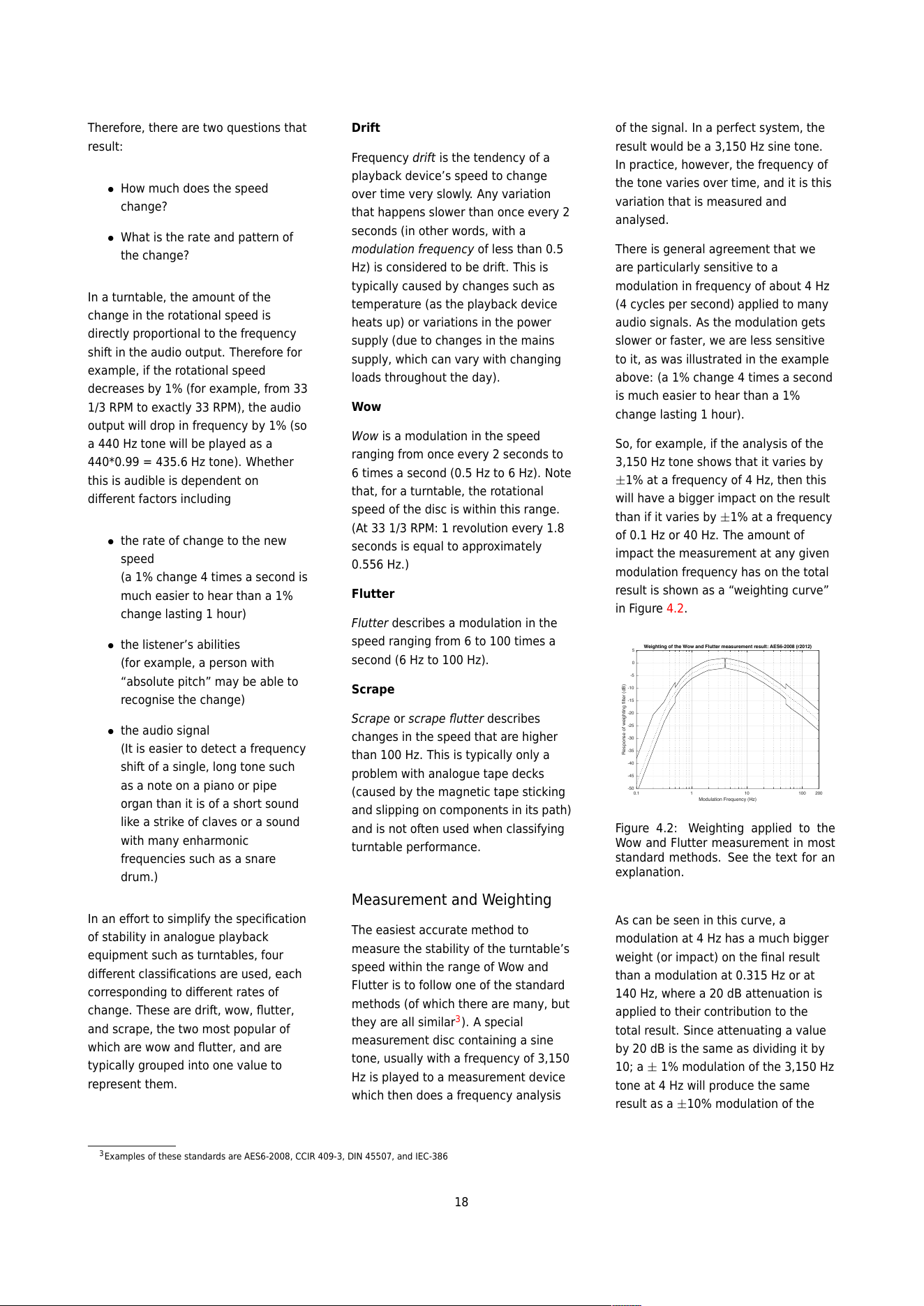
of 0.1 Hz or 40 Hz. The amount of

impact the measurement at any given

modulation frequency has on the total

result is shown as a “weighting curve”

in Figure 4.2.

0.1 1 10 100 200

Modulation Frequency (Hz)

-50

-45

-40

-35

-30

-25

-20

-15

-10

-5

Response of weighting filter (dB)

Weighting of the Wow and Flutter measurement result: AES6-2008 (r2012)

Figure 4.2: Weighting applied to the

Wow and Flutter measurement in most

standard methods. Se e the text for an

explanation.

As can be seen in this curve, a

modulation at 4 Hz has a much bigger

weight (or impact) on the ﬁnal result

than a modulation at 0.315 Hz or at

140 Hz, where a 20 dB attenuation is

applied to their contribution to the

total result. Since atten uat ing a value

by 20 dB is the same as dividing it by

10; a ± 1% modulation of the 3,150 Hz

tone at 4 Hz will produce the same

result as a ±10% modulation of the

Examples of these standards are AES6-2008, CCIR 409-3, DIN 45507, and IEC-386

3,150 Hz tone at 140 Hz, for example.

This shows just one example of why

comparing one Wow and Flutter

measurement value should be

interpreted very cautiously...

Expressing the result

When looking at a Wow and Flutter

speciﬁcation, one will see something

like <0.1%, <0.05% (DIN), or <0.1%

(AES6). Like any audio speciﬁcation, if

the details of the measurement type

are not included, then the value is

useless. For example, “W& F: <0. 1% ”

means nothing, since there is no way

to know which method was used to

arrive at this value.

If the standard is included in the

speciﬁcation (DIN or AES6, for

example), then it is still diﬃcult to

compare wow and ﬂutter values. This

is because, even when performing

identical measurements and applying

the same weighting curve shown in

Figure 4.2, there are diﬀerent methods

for arriving at the ﬁnal value. The value

that you see may be a peak value (the

maximum deviation from the average

speed), the peak-to-peak value (the

diﬀerence between the minimum and

the maximum speeds), the RMS (a

version of the average deviation from

the average speed), or something else.

The AES6-2008 standard, which is the

currently accepted method of

measuring and expressing the wow

and ﬂutter spe ciﬁ c atio n, uses a “2σ” or

“2-Sigma” method, which is a way of

looking at the peak deviation to give a

kind of “worst-case” scenario. In this

method, the 3,150 Hz tone is played

from a disc and captured for as long a

time as is possible or feasible. Firstly,

the average value of the actual

frequency of the output is found (in

theory, it’s ﬁxed at 3,150 H z, but this is

never true). Next, the short-term

variation of the actual frequency over

time is compared to the average, and

weighted using the ﬁlter shown in

Figure 4.2. The result shows the

instantaneous frequency variations

over the length of the captured signal,

relative to the average frequency

(however, the eﬀect of very slow and

very fast changes have been reduced

by the ﬁlter). Finally, the standard

deviation of the variation from the

average is calculated, and multiplied

by 2 (hence “2-Sigma”, or “two times

the standard deviation”), resulting in

the value that is shown as the

speciﬁcation. The reason two standard

deviations is chosen is that (in the

typical case where the deviation has a

Gaussian distribution) the actual Wow

& Flutter value should exceed this

value no more than 5% of the time.

The reason this method is preferred

today is that it uses a single number to

express not only the wow and ﬂutter,

but the probability of the device

reaching that value. For example, if a

device is stated to have a Wow and

Flutter of “1% (AES6)”, then the actual

deviation from the average speed will

be less than 1% for 95% of the time

you are listening to music. The

principal reason this method was not

used in the 1970s when the Beogram

4002 turntable was released is that it

requires statistical calculations applied

to a signal that was captured from the

output of the turntable, an option that

was not available 45 years ago. The

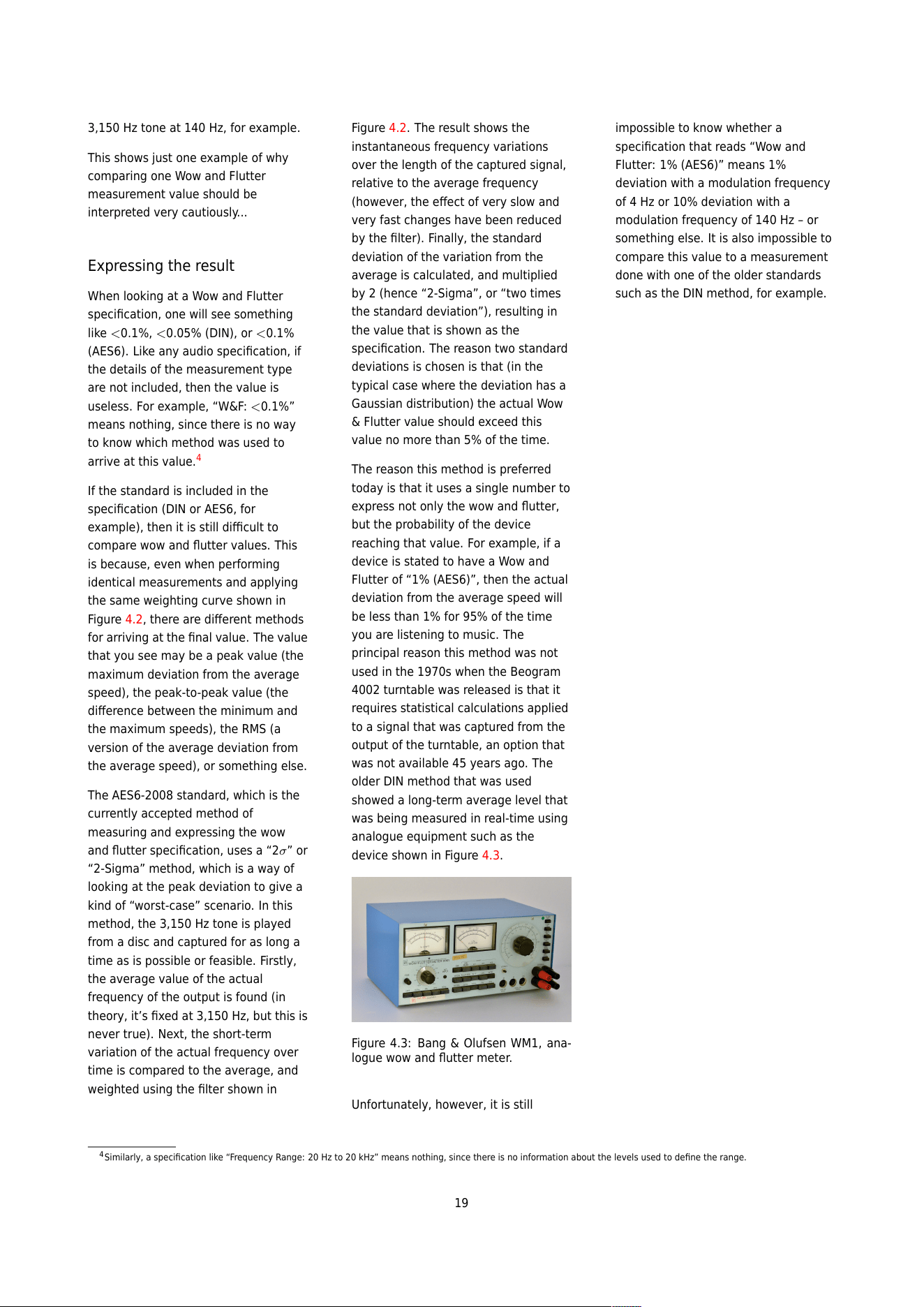
older DIN method that was used

showed a long-term average level that

was being measured in real-time using

analogue equipment such as the

device shown in Figure 4.3.

Figure 4.3: Bang & Olufsen WM1, ana-

logue wow and ﬂutter meter.

Unfortunately, however, it is still

impossible to know whether a

speciﬁcation that reads “Wow and

Flutter: 1% (AES6)” means 1%

deviation with a modulation frequency

of 4 Hz or 10% deviation with a

modulation frequency of 140 Hz – or

something else. It is also impossible to

compare this value to a measurement

done with one of the older standards

such as the DIN method, for example.

Similarly, a speciﬁcation like “Frequency Range: 20 Hz t o 20 k H z” means nothing, since there is no information abou t t he levels used to deﬁne the range.

Reading the measurement

datasheet

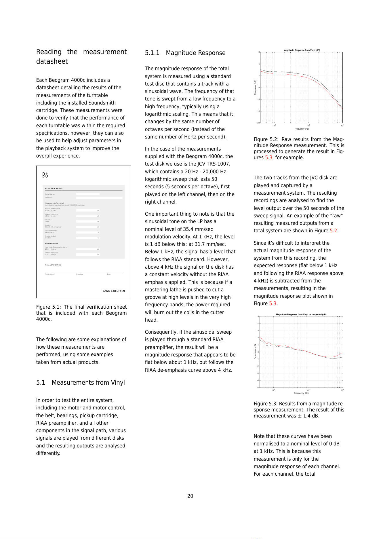
Each Beogram 4000c includes a

datasheet detailing the results of the

measurements of the turntable

including the installed Soundsmith

cartridge. These measurements were

done to verify that the performance of

each turntable was within the required

speciﬁcations, however, they can also

be used to help adjust parameters in

the playback system to improve the

overall experience.

FINAL VERIFICATION

Te st En g i ne e r

DateSignature

BEOGRAM 4000C

Serial Number

Te st Pl a c e

Measurements from Vinyl

Including the supplied Soundsmith SMMC20L cartridge

Magnitude Respon se

40 Hz - 10 kHz dB

Channel Matching

40 Hz - 10 kHz dB

Crosstalk

1 kHz dB

Rumble

DIN 45 539, Weighted dB

Wow and Flutter

AES6-2008 %

Frequency Drift

IEC 386 %

RIAA Preampliﬁer

Magnitude Respon se Deviati on

20 Hz - 20 kHz dB

Channel Matching

20 Hz - 20 kHz dB

Figure 5.1: The ﬁnal veriﬁcation s h ee t

that is included with each Beogram

4000c.

The following are some explanations of

how these measurements are

performed, using some examples

taken from actual products.

5.1 Measurements from Vinyl

In order to test the entire system,

including the motor and motor control,

the belt, bearings, pickup cartridge,

RIAA preampliﬁer, and all other

components in the signal path, various

signals are played from diﬀerent disks

and the resulting outputs are analysed

diﬀerently.

5.1.1 Magnitude Response

The magnitude response of the total

system is measured using a standard

test disc that contains a track with a

sinusoidal wave. The frequency of that

tone is swept from a low frequency to a

high frequency, typically using a

logarithmic scaling. This means that it

changes by the same number of

octaves per second (instead of the

same number of Hertz per second).

In the case of the measurements

supplied with the Beogram 4000c, the

test disk we use is the JCV TRS-1007,

which contains a 20 Hz - 20,000 Hz

logarithmic sweep that lasts 50

seconds (5 seconds per octave), ﬁrst

played on the left channel, then on the

right channel.

One important thing to note is that the

sinusoidal tone on the LP has a

nominal level of 35.4 mm/sec

modulation velocity. At 1 kHz, the level

is 1 dB below this: at 31.7 mm/sec.

Below 1 kHz, the signal has a level that

follows the RIAA standa rd. However,

above 4 kHz the signal on the disk has

a constant velocity without the RIAA

emphasis applied. This is because if a

mastering lathe is pushed to cut a

groove at high levels in the very high

frequency bands, the power required

will burn out the coils in the cutter

head.

Consequently, if the sinusoidal sweep

is played through a standard RIAA

preampliﬁer, the result will be a

magnitude response that appears to be

ﬂat below about 1 kHz, but follows the

RIAA de-emphas is cu rve ab ove 4 kH z.

Frequency (Hz)

-20

-15

-10

-5

Response (dB)

Magnitude Response from Vinyl (dB)

Figure 5.2: Raw results from the Mag-

nitude Response measurement. This is

processed to generate the result in Fig-

ures 5.3, for example.

The two tracks from the JVC disk are

played and captured by a

measurement system. The resulting

recordings are analysed to ﬁnd the

level output over the 50 seconds of the

sweep signal. An example of the “raw”

resulting measured outputs from a

total system are shown in Figure 5.2.

Since it’s diﬃcult to interpret the

actual magnitude response of the

system from this recording, the

expected response (ﬂat below 1 kHz

and following the RIAA response above

4 kHz) is subtracted from the

measurements, resulting in the

magnitude response plot shown in

Figure 5.3.

Frequency (Hz)

-5

-4

-3

-2

-1

Response (dB)

Magnitude Response from Vinyl rel. expected (dB)

Figure 5.3 : Results from a magnitude re-

sponse measurement. The result of this

measurement was ± 1.4 dB.

Note that these curves have been

normalised to a nominal level of 0 dB

at 1 kHz. This is because this

measurement is only for the

magnitude response of each channel.

For each channel, the total

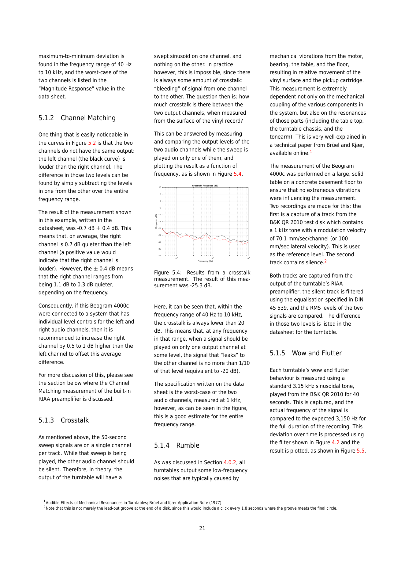
maximum-to-minimum deviation is

found in the frequency range of 40 Hz

to 10 kHz, and the worst-case of the

two channels is listed in the

“Magnitude Response” value in the

data sheet.

5.1.2 Channel Matching

One thing that is easily noticeable in

the curves in Figure 5.2 is that the two

channels do not have the same output:

the left channel (the black curve) is

louder than the right channel. The

diﬀerence in those two levels can be

found by simply subtracting the levels

in one from the other over the entire

frequency range.

The result of the measurement shown

in this example, written in the

datasheet, was -0.7 dB ± 0.4 dB. This

means that, on average, the right

channel is 0.7 dB quieter than the left

channel (a positive value would

indicate that the right channel is

louder). However, the ± 0.4 dB means

that the right channel ranges from

being 1.1 dB to 0.3 dB quieter,

depending on the frequency.

Consequently, if this Beogram 4000c

were connected to a system that has

individual level controls for the left and

right audio channels, then it is

recommended to increase the right

channel by 0.5 to 1 dB higher than the

left channel to oﬀset this average

diﬀerence.

For more discussion of this, please see

the section below where the Channel

Matching measurement of the built-in

RIAA preampliﬁer is discussed.

5.1.3 Crosstalk

As mentioned above, the 50-second

sweep signals are on a single channel

per track. While that sweep is being

played, the other audio channel should

be silent. Therefore, in theory, the

output of the turntable will have a

swept sinusoid on one channel, and

nothing on the other. In practice

however, this is impossible, since there

is always some amount of crosstalk:

“bleeding” of signal from one channel

to the other. The question then is: how

much crosstalk is there between the

two output channels, when measured

from the surface of the vinyl record?

This can be answered by measuring

and comparing the output levels of the

two audio channels while the sweep is

played on only one of them, and

plotting the result as a function of

frequency, as is shown in Figure 5.4.

Frequency (Hz)

-40

-35

-30

-25

-20

-15

-10

-5

Response (dB)

Crosstalk Response (dB)

Figure 5.4: Res ults from a crosst alk

measurement. The result of this mea-

surement was -25.3 dB.

Here, it can be seen that, within the

frequency range of 40 Hz to 10 kHz,

the crosstalk is always lower than 20

dB. This means that, at any frequency

in that range, when a signal should be

played on only one output channel at

some level, the signal that “leaks” to

the other channel is no more than 1/10

of that level (equivalent to -20 dB).

The speciﬁcation written on the data

sheet is the worst-case of the two

audio channels, measured at 1 kHz,

however, as can be seen in the ﬁgure,

this is a good estimate for the entire

frequency range.

5.1.4 Rumble

As was discussed in Section 4.0.2, all

turntables output some low-frequency

noises that are typically caused by

mechanical vibrations from the motor,

bearing, the table, and the ﬂoor,

resulting in relative movement of the

vinyl surface and the pickup cartridge.

This measurement is extremely

dependent not only on the mechanical

coupling of the various components in

the system, but also on the resonances

of those parts (including the table top,

the turntable chassis, and the

tonearm). This is very well-explained in

a technical paper from Brüel and Kjær,

available online.

The measurement of the Beogram

4000c was performed on a large, solid

table on a concrete basement ﬂoor to

ensure that no extraneous vibrations

were inﬂuencing the measurement.

Two recordings are made for this: the

ﬁrst is a capture of a track from the

B&K QR 2010 test disk which contains

a 1 kHz tone with a modulation velocity

of 70.1 mm/sec/channel (or 100

mm/sec lateral velocity). This is used

as the reference level. The second

track contains silence.

Both tracks are captured from the

output of the turntable’s RIAA

preampliﬁer, the silent track is ﬁltered

using the equalisation speciﬁed in DIN

45 539, and the RMS levels of the two

signals are compared. The diﬀerence

in those two levels is listed in the

datasheet for the turntable.

5.1.5 Wow and Flutter

Each turntable’s wow and ﬂutter

behaviour is measured using a

standard 3.15 kHz sinusoidal tone,

played from the B&K QR 2010 for 40

seconds. This is captured, and the

actual frequency of the signal is

compared to the expected 3,150 Hz for

the full duration of the recording. This

deviation over time is processed using

the ﬁlter shown in Figure 4.2 and the

result is plotted, as shown in Figure 5 .5 .

Audible Eﬀects of Mechanical Resonances in Turntables; Brüel and Kjær Application Note (1977)

Note that this is not merely the lead-out groove at the end of a disk, since this would include a click every 1.8 seconds where the groove meets the ﬁnal circle.

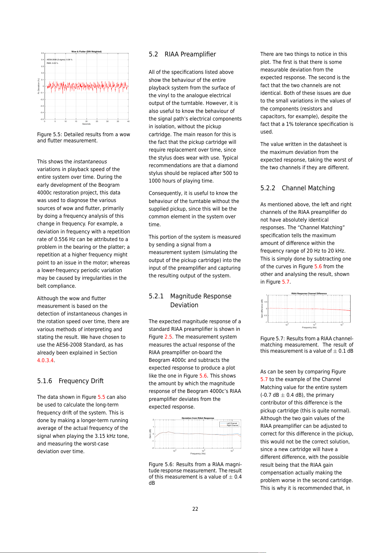
0 5 10 15 20 25 30 35 40

Seconds

-0.5

-0.4

-0.3

-0.2

-0.1

0.1

0.2

0.3

0.4

0.5

Fc Deviation (%)

Wow & Flutter (DIN Weighted)

AES6-2008 (2-sigma): 0.06 %

RMS: 0.03 %

Figure 5.5: Detailed results from a wow

and ﬂutter measurement.

This shows the instantaneous

variations in playback speed of the

entire system over time. During the

early development of the Beogram

4000c restoration project, this data

was used to diagnose the various

sources of wow and ﬂutter, primarily

by doing a frequency analysis of this

change in frequency. For example, a

deviation in frequency with a repetition

rate of 0.556 Hz can be attributed to a

problem in the bearing or the platter; a

repetition at a higher frequency might

point to an issue in the motor; whereas

a lower-frequency periodic variation

may be caused by irregularities in the

belt compliance.

Although the wow and ﬂutter

measurement is based on the

detection of instantaneous changes in

the rotation speed over time, there are

various methods of interpreting and

stating the result. We have chosen to

use the AES6-2008 Standard, as has

already been explained in Section

4.0.3.4.

5.1.6 Frequency Drift

The data shown in Figure 5.5 can also

be used to calculate the long-term

frequency drift of the system. This is

done by making a longer-term running

average of the actual frequency of the

signal when playing the 3.15 kHz tone,

and measuring the worst-case

deviation over time.

5.2 RIAA Preampliﬁer

All of the speciﬁcations listed above

show the behaviour of the entire

playback system from the surface of

the vinyl to the analogue electrical

output of the turntable. However, it is

also useful to know the behaviour of

the signal path’s electrical components

in isolation, without the pickup

cartridge. The main reason for this is

the fact that the pickup cartridge will

require replacement over time, since

the stylus does wear with use. Typical

recommendations are that a diamond

stylus should be replaced after 500 to

1000 hours of playing time.

Consequently, it is useful to know the

behaviour of the turntable without the

supplied pickup, since this will be the

common element in the system over

time.

This portion of the system is measured

by sending a signal from a

measurement system (simulating the

output of the pickup cartridge) into the

input of the preampliﬁer and capturing

the resulting output of the system.

5.2.1 Magnitude Response

Deviation

The expected magnitude response of a

standard RIAA preampliﬁer is shown in

Figure 2.5. The measurement system

measures the actual response of the

RIAA preampliﬁer on-board th e

Beogram 4000c and subtracts the

expected response to produce a plot

like the one in Figure 5.6. This shows

the amount by which the magnitude

response of the Beogram 4000c’s RIAA

preampliﬁer deviates from the

expected response.

Frequency (Hz)

-2

-1

Gain (dB)

Deviation from RIAA Response

Left Channel

Right Channel

Figure 5.6: Results from a RIAA magni-

tude response measurement. The result

of this measurement is a value of ± 0.4

There are two things to notice in this

plot. The ﬁrst is that there is some

measurable deviation from the

expected response. The second is the

fact that the two channels are not

identical. Both of these issues are due

to the small variations in the values of

the components (resistors and

capacitors, for example), despite the

fact that a 1% tolerance speciﬁcation is

used.

The value written in the datasheet is

the maximum deviation from the

expected response, taking the worst of

the two channels if they are diﬀerent.

5.2.2 Channel Matching

As mentioned above, the left and right

channels of the RIAA preampliﬁer do

not have absolutely identical

responses. The “Channel Matching”

speciﬁcation tells the maximum

amount of diﬀerence within the

frequency range of 20 Hz to 20 kHz.

This is simply done by subtracting one

of the curves in Figure 5.6 from the

other and analysing the result, shown

in Figure 5.7.

Frequency (Hz)

-1

-0.5

0.5

Gain difference (dB)

RIAA Response Channel Difference

Figure 5.7: Results from a RIAA channe l-

matching measurement. The result of

this measurement is a value of ± 0.1 dB

As can be seen by comparing Figure

5.7 to the example of the Channel

Matching value for the entire system

(-0.7 dB ± 0.4 dB), the primary

contributor of this diﬀerence is the

pickup cartridge (this is quite normal).

Although the two gain values of the

RIAA preampliﬁer can be adjusted to

correct for this diﬀerence in the pickup,

this would not be the correct solution,

since a new cartridge will have a

diﬀerent diﬀerence, with the possible

result being that the RIAA gain

compensation actually making the

problem worse in the second cartridge.

This is why it is recommended that, in

cases where you wish to correct for the

gain oﬀset, this should be done as a

“temporary” measure in the playback

system.

Attentive readers may notice some

small spikes in the plot in Figure 5.7.

These are merely artefacts of the

measurement system, revealed by the

subtraction of the two curves. They are

not reﬂective of actual diﬀerences in

the preampliﬁer’s responses.

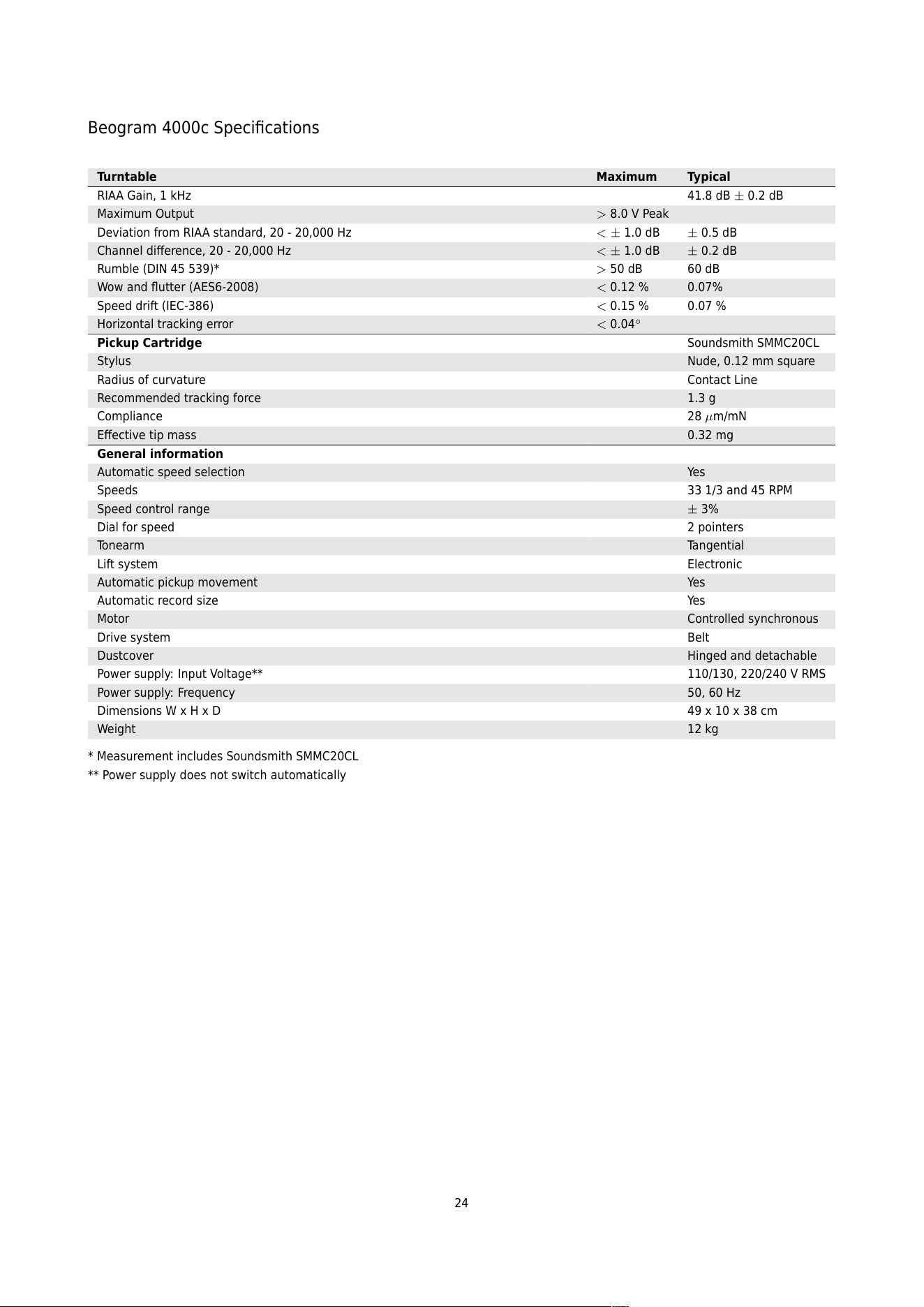
Beogram 4000c Speciﬁcations

Turntable Maximum Typical

RIAA Gain, 1 kHz 41.8 dB ± 0.2 dB

Maximum Output > 8.0 V Peak

Deviation from RIAA standard, 20 - 20,000 Hz < ± 1.0 dB ± 0.5 dB

Channel diﬀerence, 20 - 20,000 Hz < ± 1.0 dB ± 0.2 dB

Rumble (DIN 45 539)* > 50 dB 60 dB

Wow and ﬂutter (AES6-2008) < 0.12 % 0.07%

Speed drift (IEC-386) < 0.15 % 0.07 %

Horizontal tracking error < 0.04

◦

Pickup Cartridge Soundsmith SMMC20CL

Stylus Nude, 0.12 mm square

Radius of curvature Contact Line

Recommended tracking force 1.3 g

Compliance 28 µm/mN

Eﬀective tip mass 0.32 mg

General infor ma tio n

Automatic speed selection Yes

Speeds 33 1/3 and 45 RPM

Speed control range ± 3%

Dial for speed 2 pointers

Tonearm Tangential

Lift system Electronic

Automatic pickup movement Yes

Automatic record size Yes

Motor Controlled synchronous

Drive system Belt

Dustcover Hinged and detachable

Power supply: Input Voltage** 110/130, 220/240 V RMS

Power supply: Frequency 50, 60 Hz

Dimensions W x H x D 49 x 10 x 38 cm

Weight 12 kg

* Measurement includes Soundsmith SMMC20CL

** Power supply does not switch automatically

Bang & Olufsen BEOGRAM 4000C A Classic. Reborn.

Product's Documents

Technical Sound Guide

Specifications

Bang & Olufsen BEOGRAM Questions and Answers