10/25/02 © 2001, 2002 Texas Instruments
TI
TI
-
83 Plus /
TI-83 Plus Silver Edition
Graphing Calculator Guidebook
On/Off Graphing a function
Menus Modes
Using parentheses Lists
Tables Data and lists
Matrices Split screen
Inferential statistics Archiving/Unarchiving
Programming Menu maps
Sending and receiving Troubleshooting
Formulas Support and service
More Information
First Steps
Creating…
Beyond the Basics

TI-83 Plus © 2001, 2002 Texas Instruments
Important
Texas Instruments makes no warranty, either expressed or implied,
including but not limited to any implied warranties of merchantability and
fitness for a particular purpose, regarding any programs or book
materials and makes such materials available solely on an “as-is” basis.
In no event shall Texas Instruments be liable to anyone for special,
collateral, incidental, or consequential damages in connection with or
arising out of the purchase or use of these materials, and the sole and
exclusive liability of Texas Instruments, regardless of the form of action,
shall not exceed the purchase price of this equipment. Moreover, Texas
Instruments shall not be liable for any claim of any kind whatsoever
against the use of these materials by any other party.
Windows is a registered trademark of Microsoft Corporation.
Macintosh is a registered trademark of Apple Computer, Inc.

TI-83 Plus © 2001, 2002 Texas Instruments
US FCC Information Concerning Radio
Frequency Interference
This equipment has been tested and found to comply with the limits for a
Class B digital device, pursuant to Part 15 of the FCC rules. These limits
are designed to provide reasonable protection against harmful
interference in a residential installation. This equipment generates, uses,
and can radiate radio frequency energy and, if not installed and used in
accordance with the instructions, may cause harmful interference with
radio communications. However, there is no guarantee that interference
will not occur in a particular installation.
If this equipment does cause harmful interference to radio or television
reception, which can be determined by turning the equipment off and on,
you can try to correct the interference by one or more of the following
measures:
•
Reorient or relocate the receiving antenna.
•
Increase the separation between the equipment and receiver.
•
Connect the equipment into an outlet on a circuit different from that to
which the receiver is connected.
•
Consult the dealer or an experienced radio/television technician for
help.
Caution:
Any changes or modifications to this equipment not expressly
approved by Texas Instruments may void your authority to operate the
equipment.

TI-83 Plus Operating the TI-83 Plus Silver Edition 1
Chapter 1:
Operating the TI-83 Plus Silver Edition
Documentation Conventions
In the body of this guidebook, TI-83 Plus (in silver) refers to the
TI-83 Plus Silver Edition. Sometimes, as in Chapter 19, the full
name TI-83 Plus Silver Edition is used to distinguish it from the
TI-83 Plus.
All the instructions and examples in this guidebook also work for
the TI-83 Plus. All the functions of the TI-83 Plus Silver Edition and the
TI-83 Plus are the same. The two calculators differ only in available RAM
memory and Flash application ROM memory.

TI-83 Plus Operating the TI-83 Plus Silver Edition 2
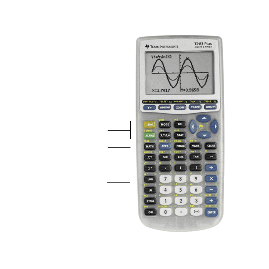
TI-83 Plus Keyboard
Generally, the keyboard is divided into these zones: graphing keys,
editing keys, advanced function keys, and scientific calculator keys.
Keyboard Zones
Graphing
— Graphing keys access the interactive graphing features.
Editing
— Editing keys allow you to edit expressions and values.
Advanced
— Advanced function keys display menus that access the
advanced functions.
Scientific
— Scientific calculator keys access the capabilities of a
standard scientific calculator.
TI-83 Plus Operating the TI-83 Plus Silver Edition 3
TI-83 Plus
Editing Keys
Advanced
Function Keys
Scientific
Calculator Keys
Graphing Keys
Colors may vary in actual product.

TI-83 Plus Operating the TI-83 Plus Silver Edition 4
Using the Color
.
Coded Keyboard
The keys on the TI-83 Plus are color-coded to help you easily locate the
key you need.
The light gray keys are the number keys. The blue keys along the right side
of the keyboard are the common math functions. The blue keys across the
top set up and display graphs. The blue
Œ
key provides access to
applications such as the Finance application.
The primary function of each key is printed on the keys. For example,
when you press
, the
MATH
menu is displayed.
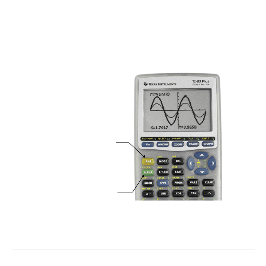
Using the
y
and
ƒ
Keys
The secondary function of each key is printed in yellow above the key.
When you press the yellow
y
key, the character, abbreviation, or word
printed in yellow above the other keys becomes active for the next
keystroke. For example, when you press
y
and then
, the
TEST
menu is displayed. This guidebook describes this keystroke combination
as
y
:
.
TI-83 Plus Operating the TI-83 Plus Silver Edition 5
The alpha function of each key is printed in green above the key. When
you press the green
ƒ
key, the alpha character printed in green
above the other keys becomes active for the next keystroke. For
example, when you press
ƒ
and then
, the letter
A
is entered.
This guidebook describes this keystroke combination as
ƒ
[
A
].
The
y
key
accesses the
second function
printed in yellow
above each ke
y
.
The
ƒ
key
accesses the alpha
function printed in
green above each
key.
TI-83 Plus Operating the TI-83 Plus Silver Edition 6
Turning On and Turning Off the TI-83 Plus
Turning On the Calculator
To turn on the TI-83 Plus, press
É
.
•
If you previously had turned off the
calculator by pressing
y
M
, the
TI-83 Plus displays the home screen as it
was when you last used it and clears any
error.
•
If Automatic Power Down™ (APD
é
) had previously turned off the
calculator, the TI-83 Plus will return exactly as you left it, including the
display, cursor, and any error.
•
If the TI-83 Plus is turned off and you connect it to another calculator
or personal computer, the TI-83 Plus will “wake up” when you
complete the connection.
•
If the TI-83 Plus is turned off and connected to another calculator or
personal computer, any communication activity will “wake up” the
TI-83 Plus.
To prolong the life of the batteries, APD turns off the TI-83 Plus
automatically after about five minutes without any activity.

TI-83 Plus Operating the TI-83 Plus Silver Edition 7
Turning Off the Calculator
To turn off the TI-83 Plus manually, press
y
M
.
•
All settings and memory contents are retained by Constant
Memory
TM
.
•
Any error condition is cleared.
Batteries
The TI-83 Plus uses four AAA alkaline batteries and has a user-
replaceable backup lithium battery (CR1616 or CR1620). To replace
batteries without losing any information stored in memory, follow the
steps in Appendix B.

TI-83 Plus Operating the TI-83 Plus Silver Edition 8
Setting the Display Contrast
Adjusting the Display Contrast
You can adjust the display contrast to suit your viewing angle and lighting
conditions. As you change the contrast setting, a number from
0
(lightest)
to
9
(darkest) in the top-right corner indicates the current level. You may
not be able to see the number if contrast is too light or too dark.
Note: The TI-83 Plus has 40 contrast settings, so each number
0
through
9
represents four settings.
The TI-83 Plus retains the contrast setting in memory when it is turned
off.
To adjust the contrast, follow these steps.
1. Press and release the
y
key.
2. Press and hold
†
or
}
, which are below and above the contrast
symbol (yellow, half-shaded circle).
•
†
lightens the screen.
•
}
darkens the screen.

TI-83 Plus Operating the TI-83 Plus Silver Edition 9
Note:
If you adjust the contrast setting to
0
, the display may become completely
blank. To restore the screen, press and release
y
, and then press and hold
}
until the display reappears.
When to Replace Batteries
When the batteries are low, a low-battery message is displayed when
you:
•
Turn on the calculator.
•
Download a new application.
•
Attempt to upgrade to new software.
To replace the batteries without losing any information in memory, follow
the steps in Appendix B.
Generally, the calculator will continue to operate for one or two weeks
after the low-battery message is first displayed. After this period, the
TI-83 Plus will turn off automatically and the unit will not operate.
Batteries must be replaced. All memory should be retained.
Note:
The operating period following the first low-battery message could be
longer than two weeks if you use the calculator infrequently.

TI-83 Plus Operating the TI-83 Plus Silver Edition 10
The Display
Types of Displays
The TI-83 Plus displays both text and graphs. Chapter 3 describes
graphs. Chapter 9 describes how the TI-83 Plus can display a
horizontally or vertically split screen to show graphs and text
simultaneously.
Home Screen
The home screen is the primary screen of the TI-83 Plus. On this screen,
enter instructions to execute and expressions to evaluate. The answers
are displayed on the same screen.
Displaying Entries and Answers
When text is displayed, the TI-83 Plus screen can display a maximum of
8 lines with a maximum of 16 characters per line. If all lines of the display
are full, text scrolls off the top of the display. If an expression on the
home screen, the
Y=
editor (Chapter 3), or the program editor
(Chapter 16) is longer than one line, it wraps to the beginning of the next
line. In numeric editors such as the window screen (Chapter 3), a long
expression scrolls to the right and left.
TI-83 Plus Operating the TI-83 Plus Silver Edition 11
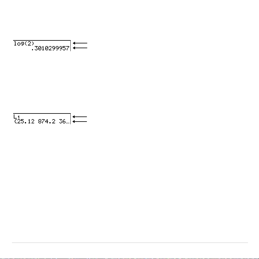
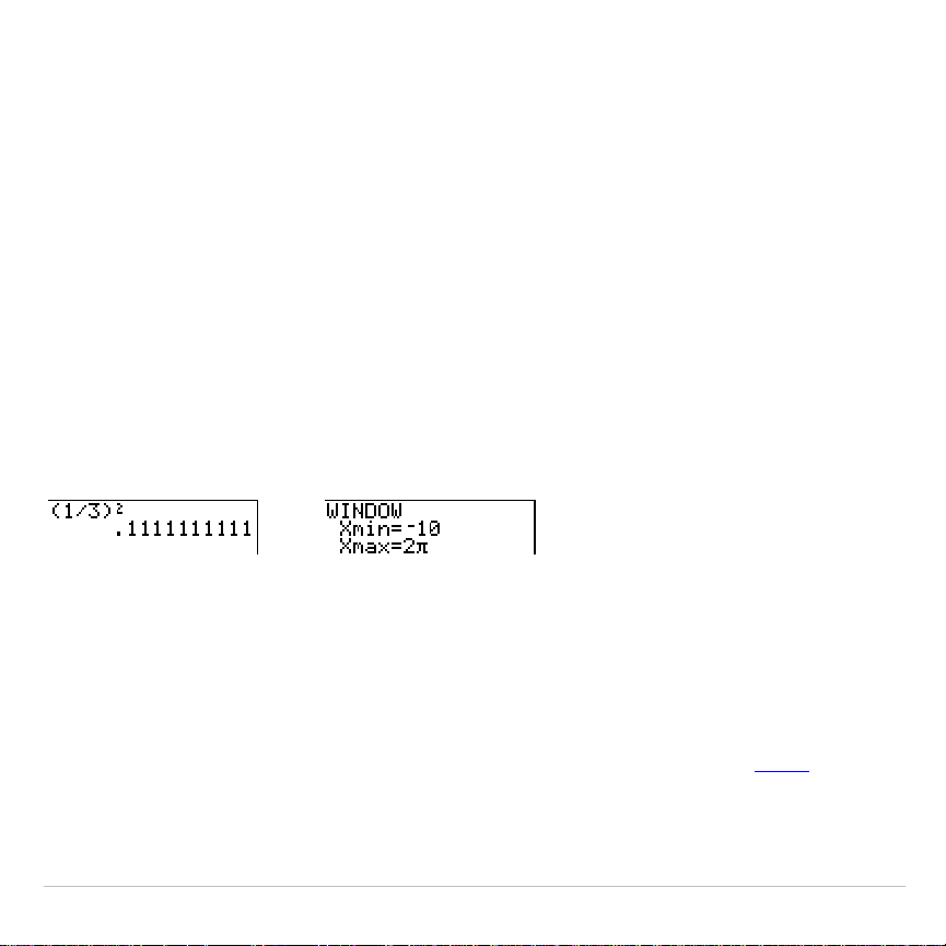
When an entry is executed on the home screen, the answer is displayed
on the right side of the next line.
Entry
Answer
The mode settings control the way the TI-83 Plus interprets expressions
and displays answers.
If an answer, such as a list or matrix, is too long to display entirely on
one line, an ellipsis (
...
) is displayed to the right or left. Press
~
and
|
to
display the answer.
Entry
Answer
Returning to the Home Screen
To return to the home screen from any other screen, press
y
5
.
Busy Indicator
When the TI-83 Plus is calculating or graphing, a vertical moving line is
displayed as a busy indicator in the top-right corner of the screen. When
you pause a graph or a program, the busy indicator becomes a vertical
moving dotted line.

TI-83 Plus Operating the TI-83 Plus Silver Edition 12
Display Cursors
In most cases, the appearance of the cursor indicates what will happen
when you press the next key or select the next menu item to be pasted
as a character.
Cursor Appearance Effect of Next Keystroke
Entry Solid rectangle
$
A character is entered at the cursor; any
existing character is overwritten
Insert Underline
__
A character is inserted in front of the cursor
location
Second Reverse arrow
Þ
A 2nd character (yellow on the keyboard) is
entered or a 2nd operation is executed
Alpha Reverse A
Ø
An alpha character (green on the keyboard)
is entered or
SOLVE
is executed
Full Checkerboard
rectangle
#
No entry; the maximum characters are
entered at a prompt or memory is full
If you press
ƒ
during an insertion, the cursor becomes an underlined
A
(
A
). If you press
y
during an insertion, the underlined cursor becomes
an underlined
#
(
#
).
Graphs and editors sometimes display additional cursors, which are
described in other chapters.
TI-83 Plus Operating the TI-83 Plus Silver Edition 13
Entering Expressions and Instructions
What Is an Expression?
An expression is a group of numbers, variables, functions and their
arguments, or a combination of these elements. An expression evaluates
to a single answer. On the TI-83 Plus, you enter an expression in the
same order as you would write it on paper. For example,
p
R
2
is an
expression.
You can use an expression on the home screen to calculate an answer.
In most places where a value is required, you can use an expression to
enter a value.
Entering an Expression
To create an expression, you enter numbers, variables, and functions
from the keyboard and menus. An expression is completed when you
press
Í
, regardless of the cursor location. The entire expression is
evaluated according to Equation Operating System (EOS
é
)
rules
, and
the answer is displayed.
TI-83 Plus Operating the TI-83 Plus Silver Edition 14
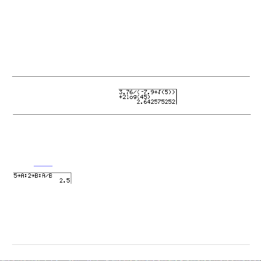
Most TI-83 Plus functions and operations are symbols comprising
several characters. You must enter the symbol from the keyboard or a
menu; do not spell it out. For example, to calculate the log of 45, you
must press
«
45
. Do not enter the letters
L
,
O
, and
G
. If you enter
LOG
,
the TI-83 Plus interprets the entry as implied multiplication of the
variables
L
,
O
, and
G
.
Calculate 3.76 ÷ (
L
7.9 +
‡
5) + 2 log 45.
3
Ë
76
¥
£
Ì
7
Ë
9
Ã
y
C
5
¤
¤
Ã
2
«
45
¤
Í
Multiple Entries on a Line
To enter two or more expressions or instructions on a line, separate
them with colons (
ƒ
[
:
]). All instructions are stored together in last
entry (
ENTRY
) .
Entering a Number in Scientific Notation
To enter a number in scientific notation, follow these steps.
TI-83 Plus Operating the TI-83 Plus Silver Edition 15
1. Enter the part of the number that precedes the exponent. This value
can be an expression.
2. Press
y
D
.
å
is pasted to the cursor location.
3. If the exponent is negative, press
Ì
, and then enter the exponent,
which can be one or two digits.
When you enter a number in scientific notation, the TI-83 Plus does not
automatically display answers in scientific or engineering notation. The
mode settings
and the size of the number determine the display format.
Functions
A function returns a value. For example,
÷
,
L
,
+
,
‡
(
, and
log(
are the
functions in the example on the previous page. In general, the first letter of
each function is lowercase on the TI-83 Plus. Most functions take at least
one argument, as indicated by an open parenthesis (
(
) following the
name. For example,
sin(
requires one argument,
sin(
value
)
.

TI-83 Plus Operating the TI-83 Plus Silver Edition 16
Instructions
An instruction initiates an action. For example,
ClrDraw
is an instruction
that clears any drawn elements from a graph. Instructions cannot be
used in expressions. In general, the first letter of each instruction name
is uppercase. Some instructions take more than one argument, as
indicated by an open parenthesis (
(
) at the end of the name. For
example,
Circle(
requires three arguments,
Circle(
X
,
Y
,
radius
)
.
Interrupting a Calculation
To interrupt a calculation or graph in progress, which is indicated by the
busy indicator, press
É
.
When you interrupt a calculation, a menu is displayed.
•
To return to the home screen, select
1:Quit
.
•
To go to the location of the interruption, select
2:Goto
.
When you interrupt a graph, a partial graph is displayed.
•
To return to the home screen, press
‘
or any nongraphing key.
•
To restart graphing, press a graphing key or select a graphing
instruction.

TI-83 Plus Operating the TI-83 Plus Silver Edition 17
TI-83 Plus Edit Keys
Keystrokes Result
~
or
|
Moves the cursor within an expression; these keys repeat.
}
or
†
Moves the cursor from line to line within an expression that
occupies more than one line; these keys repeat.
On the top line of an expression on the home screen,
}
moves
the cursor to the beginning of the expression.
On the bottom line of an expression on the home screen,
†
moves the cursor to the end of the expression.
y
|
Moves the cursor to the beginning of an expression.
y
~
Moves the cursor to the end of an expression.
Í
Evaluates an expression or executes an instruction.
‘
On a line with text on the home screen, clears the current line.
On a blank line on the home screen, clears everything on the
home screen.
In an editor, clears the expression or value where the cursor is
located; it does not store a zero.
{
Deletes a character at the cursor; this key repeats.
y
6
Changes the cursor to an underline (
__
); inserts characters in
front of the underline cursor; to end insertion, press
y
6
or
press
|
,
}
,
~
, or
†
.

TI-83 Plus Operating the TI-83 Plus Silver Edition 18
Keystrokes Result
y
Changes the cursor to
Þ
; the next keystroke performs a
2nd
operation (an operation in yellow above a key and to the left); to
cancel
2nd
, press
y
again.
ƒ
Changes the cursor to
Ø
; the next keystroke pastes an alpha
character (a character in green above a key and to the right) or
executes
SOLVE
(Chapters 10 and 11); to cancel
ƒ
, press
ƒ
or press
|
,
}
,
~
, or
†
.
y
7
Changes the cursor to
Ø
; sets alpha-lock; subsequent
keystrokes (on an alpha key) paste alpha characters; to cancel
alpha-lock, press
ƒ
. If you are prompted to enter a name
such as for a group or a program, alpha-lock is set automatically.
„
Pastes an
X
in
Func
mode, a
T
in
Par
mode, a
q
in
Pol
mode, or
an
n
in
Seq
mode with one keystroke.

TI-83 Plus Operating the TI-83 Plus Silver Edition 19
Setting Modes
Checking Mode Settings
Mode settings control how the TI-83 Plus displays and interprets
numbers and graphs. Mode settings are retained by the Constant
Memory feature when the TI-83 Plus is turned off. All numbers, including
elements of matrices and lists, are displayed according to the current
mode settings.
To display the mode settings, press
z
. The current settings are
highlighted. Defaults are highlighted below. The following pages describe
the mode settings in detail.
Normal Sci Eng
Numeric notation
Float 0123456789
Number of decimal places
Radian Degree
Unit of angle measure
Func Par Pol Seq
Type of graphing
Connected Dot
Whether to connect graph points
Sequential Simul
Whether to plot simultaneously
Real a+bi re^
q
i
Real, rectangular complex, or polar complex
Full Horiz G-T
Full screen, two split-screen modes

TI-83 Plus Operating the TI-83 Plus Silver Edition 20
Changing Mode Settings
To change mode settings, follow these steps.
1. Press
†
or
}
to move the cursor to the line of the setting that you
want to change.
2. Press
~
or
|
to move the cursor to the setting you want.
3. Press
Í
.
Setting a Mode from a Program
You can set a mode from a program by entering the name of the mode
as an instruction; for example,
Func
or
Float
. From a blank program
command line, select the mode setting from the mode screen; the
instruction is pasted to the cursor location.
Normal, Sci, Eng
Notation modes only affect the way an answer is displayed on the home
screen. Numeric answers can be displayed with up to 10 digits and a
two-digit exponent. You can enter a number in any format.

TI-83 Plus Operating the TI-83 Plus Silver Edition 21
Normal
notation mode is the usual way we express numbers, with digits
to the left and right of the decimal, as in
12345.67
.
Sci
(scientific) notation mode expresses numbers in two parts. The
significant digits display with one digit to the left of the decimal. The
appropriate power of 10 displays to the right of
E
, as in
1.234567E4
.
Eng
(engineering) notation mode is similar to scientific notation.
However, the number can have one, two, or three digits before the
decimal; and the power-of-10 exponent is a multiple of three, as in
12.34567E3
.
Note: If you select
Normal
notation, but the answer cannot display in 10 digits
(or the absolute value is less than .001), the TI-83 Plus expresses the answer in
scientific notation.
Float, 0123456789
Float
(floating) decimal mode displays up to 10 digits, plus the sign and
decimal.
0123456789
(fixed) decimal mode specifies the number of digits (
0
through
9
) to display to the right of the decimal. Place the cursor on the
desired number of decimal digits, and then press
Í
.
The decimal setting applies to
Normal
,
Sci
, and
Eng
notation modes.

TI-83 Plus Operating the TI-83 Plus Silver Edition 22
The decimal setting applies to these numbers:
•
An answer displayed on the home screen
•
Coordinates on a graph (Chapters 3, 4, 5, and 6)
•
The
Tangent(
DRAW
instruction equation of the line,
x
, and
dy/dx
values (Chapter 8)
•
Results of
CALCULATE
operations (Chapters 3, 4, 5, and 6)
•
The regression equation stored after the execution of a regression
model (Chapter 12)
Radian, Degree
Angle modes control how the TI-83 Plus interprets angle values in
trigonometric functions and polar/rectangular conversions.
Radian
mode interprets angle values as radians. Answers display in
radians.
Degree
mode interprets angle values as degrees. Answers display in
degrees.

TI-83 Plus Operating the TI-83 Plus Silver Edition 23
Func, Par, Pol, Seq
Graphing modes define the graphing parameters. Chapters 3, 4, 5, and 6
describe these modes in detail.
Func
(function) graphing mode plots functions, where
Y
is a function of
X
(Chapter 3).
Par
(parametric) graphing mode plots relations, where
X
and
Y
are
functions of
T
(Chapter 4).
Pol
(polar) graphing mode plots functions, where
r
is a function of
q
(Chapter 5).
Seq
(sequence) graphing mode plots sequences (Chapter 6).
Connected, Dot
Connected
plotting mode draws a line connecting each point calculated
for the selected functions.
Dot
plotting mode plots only the calculated points of the selected
functions.

TI-83 Plus Operating the TI-83 Plus Silver Edition 24
Sequential, Simul
Sequential
graphing-order mode evaluates and plots one function
completely before the next function is evaluated and plotted.
Simul
(simultaneous) graphing-order mode evaluates and plots all
selected functions for a single value of
X
and then evaluates and plots
them for the next value of
X
.
Note: Regardless of which graphing mode is selected, the TI-83 Plus will
sequentially graph all stat plots before it graphs any functions.
Real, a+b
i
, re^
q
i
Real
mode does not display complex results unless complex numbers
are entered as input.
Two complex modes display complex results.
•
a+b
i
(rectangular complex mode) displays complex numbers in the
form a+b
i
.
•
re^
q
i
(polar complex mode) displays complex numbers in the form
re^
q
i
.

TI-83 Plus Operating the TI-83 Plus Silver Edition 25
Full, Horiz, G
.
T
Full
screen mode uses the entire screen to display a graph or edit
screen.
Each split-screen mode displays two screens simultaneously.
•
Horiz
(horizontal) mode displays the current graph on the top half of
the screen; it displays the home screen or an editor on the bottom
half (Chapter 9).
•
G
.
T
(graph-table) mode displays the current graph on the left half of
the screen; it displays the table screen on the right half (Chapter 9).

TI-83 Plus Operating the TI-83 Plus Silver Edition 26
Using TI-83 Plus Variable Names
Variables and Defined Items
On the TI-83 Plus you can enter and use several types of data, including
real and complex numbers, matrices, lists, functions, stat plots, graph
databases, graph pictures, and strings.
The TI-83 Plus uses assigned names for variables and other items
saved in memory. For lists, you also can create your own five-character
names.
Variable Type Names
Real numbers
A
,
B
, ... ,
Z
Complex numbers
A
,
B
, ... ,
Z
Matrices
ã
A
ä
,
ã
B
ä
,
ã
C
ä
, ... ,
ã
J
ä
Lists
L1
,
L2
,
L3
,
L4
,
L5
,
L6
, and user-defined names
Functions
Y1
,
Y2
, . . . ,
Y9
,
Y0
Parametric equations
X1T
and
Y1T
, . . . ,
X6T
and
Y6T
Polar functions
r1
,
r2
,
r3
,
r4
,
r5
,
r6
Sequence functions
u
,
v
,
w
Stat plots
Plot1, Plot2, Plot3
Graph databases
GDB1
,
GDB2
, . . . ,
GDB9
,
GDB0

TI-83 Plus Operating the TI-83 Plus Silver Edition 27
Variable Type Names
Graph pictures
Pic1
,
Pic2
, ... ,
Pic9
,
Pic0
Strings
Str1
,
Str2
, ... ,
Str9
,
Str0
Apps Applications
AppVars Application variables
Groups Grouped variables
System variables
Xmin
,
Xmax
, and others
Notes about Variables
•
You can create as many list names as memory will allow
(Chapter 11).
•
Programs have user-defined names and share memory with
variables (Chapter 16).
•
From the home screen or from a program, you can store to matrices
(Chapter 10), lists (Chapter 11), strings (Chapter 15), system
variables such as
Xmax
(Chapter 1),
TblStart
(Chapter 7), and all
Y=
functions (Chapters 3, 4, 5, and 6).
•
From an editor, you can store to matrices, lists, and
Y=
functions
(Chapter 3).
•
From the home screen, a program, or an editor, you can store a
value to a matrix element or a list element.

TI-83 Plus Operating the TI-83 Plus Silver Edition 28
•
You can use
DRAW STO
menu items to store and recall graph
databases and pictures (Chapter 8).
•
Although most variables can be archived, system variables including
r, t, x, y, and
q
cannot be archived (Chapter 18)
•
Apps
are independent applications.which are stored in Flash ROM.
AppVars
is a variable holder used to store variables created by
independent applications. You cannot edit or change variables in
AppVars
unless you do so through the application which created
them.
TI-83 Plus Operating the TI-83 Plus Silver Edition 29
Storing Variable Values
Storing Values in a Variable
Values are stored to and recalled from memory using variable names.
When an expression containing the name of a variable is evaluated, the
value of the variable at that time is used.
To store a value to a variable from the home screen or a program using
the
¿
key, begin on a blank line and follow these steps.
1. Enter the value you want to store. The value can be an expression.
2. Press
¿
.
!
is copied to the cursor location.
3. Press
ƒ
and then the letter of the variable to which you want to
store the value.
4. Press
Í
. If you entered an expression, it is evaluated. The value
is stored to the variable.
TI-83 Plus Operating the TI-83 Plus Silver Edition 30
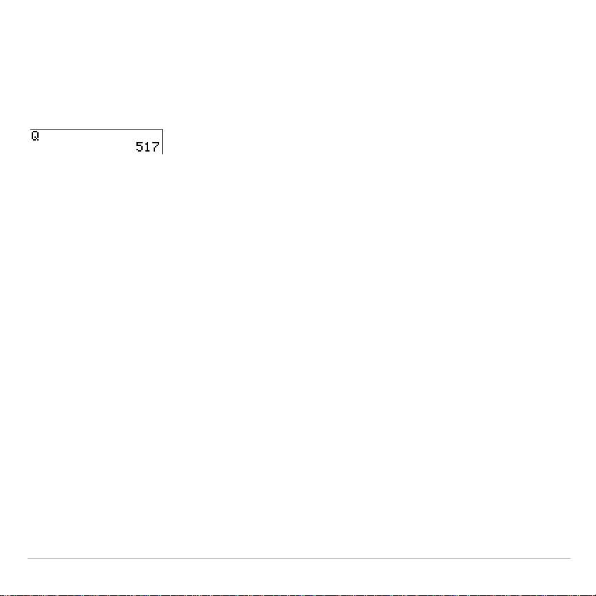
Displaying a Variable Value
To display the value of a variable, enter the name on a blank line on the
home screen, and then press
Í
.
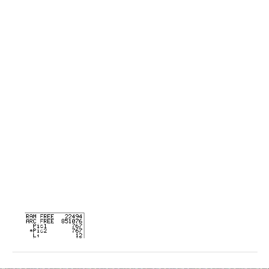
Archiving Variables (Archive, Unarchive)
You can archive data, programs, or other variables in a section of
memory called user data archive where they cannot be edited or deleted
inadvertently. Archived variables are indicated by asterisks (*) to the left
of the variable names. Archived variables cannot be edited or executed.
They can only be seen and unarchived. For example, if you archive list
L1, you will see that L1 exists in memory but if you select it and paste the
name L1 to the home screen, you won’t be able to see its contents or
edit it until they are unarchived.
.

TI-83 Plus Operating the TI-83 Plus Silver Edition 31
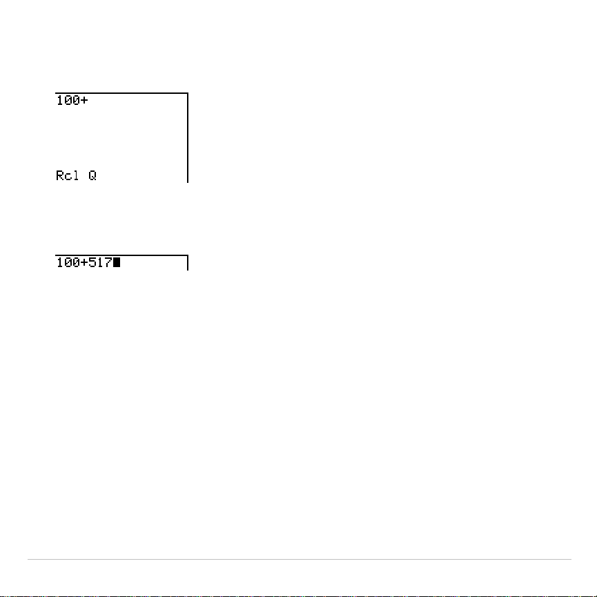
Recalling Variable Values
Using Recall (RCL)
To recall and copy variable contents to the current cursor location, follow
these steps. To leave
RCL
, press
‘
.
1.Press
y
ã
RCLä
.
RCL
and the edit cursor are displayed on the bottom
line of the screen.
2. Enter the name of the variable in any of five ways.
•
Press
ƒ
and then the letter of the variable.
•
Press
y
ãLISTä
, and then select the name of the list, or press
y
[
L
n
].
•
Press
y
>
, and then select the name of the matrix.
•
Press
to display the
VARS
menu or
~
to display the
VARS Y
.
VARS
menu; then select the type and then the name of the
variable or function.
•
Press
|
, and then select the name of the program (in the
program editor only).
TI-83 Plus Operating the TI-83 Plus Silver Edition 32
The variable name you selected is displayed on the bottom line and
the cursor disappears.
3. Press
Í
. The variable contents are inserted where the cursor
was located before you began these steps.
Note:
You can edit the characters pasted to the expression without
affecting the value in memory.
TI-83 Plus Operating the TI-83 Plus Silver Edition 33
ENTRY (Last Entry) Storage Area
Using ENTRY (Last Entry)
When you press
Í
on the home screen to evaluate an expression or
execute an instruction, the expression or instruction is placed in a
storage area called
ENTRY
(last entry). When you turn off the TI-83 Plus,
ENTRY
is retained in memory.
To recall
ENTRY
, press
y
[
. The last entry is pasted to the current
cursor location, where you can edit and execute it. On the home screen
or in an editor, the current line is cleared and the last entry is pasted to
the line.
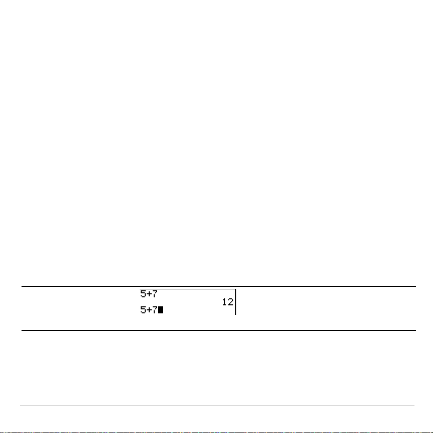
Because the TI-83 Plus updates
ENTRY
only when you press
Í
, you
can recall the previous entry even if you have begun to enter the next
expression.
5
Ã
7
Í
y
[
TI-83 Plus Operating the TI-83 Plus Silver Edition 34
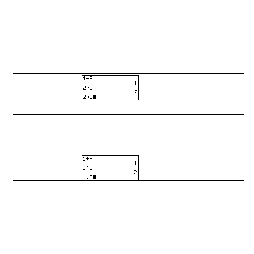
Accessing a Previous Entry
The TI-83 Plus retains as many previous entries as possible in
ENTRY
, up
to a capacity of 128 bytes. To scroll those entries, press
y
[
repeatedly. If a single entry is more than 128 bytes, it is retained for
ENTRY
, but it cannot be placed in the
ENTRY
storage area.
1
¿
ƒ
A
Í
2
¿
ƒ
B
Í
y
[
If you press
y
[
after displaying the oldest stored entry, the
newest stored entry is displayed again, then the next-newest entry, and
so on.
y
[
Reexecuting the Previous Entry
After you have pasted the last entry to the home screen and edited it (if
you chose to edit it), you can execute the entry. To execute the last
entry, press
Í
.
TI-83 Plus Operating the TI-83 Plus Silver Edition 35
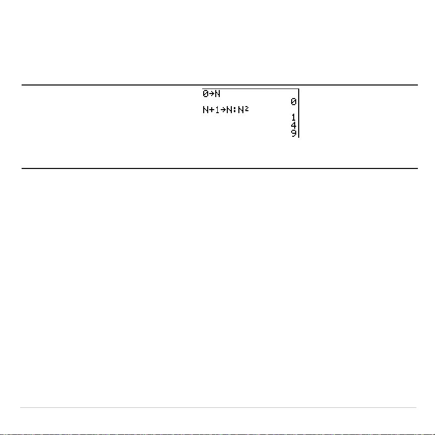
To reexecute the displayed entry, press
Í
again. Each reexecution
displays an answer on the right side of the next line; the entry itself is not
redisplayed.
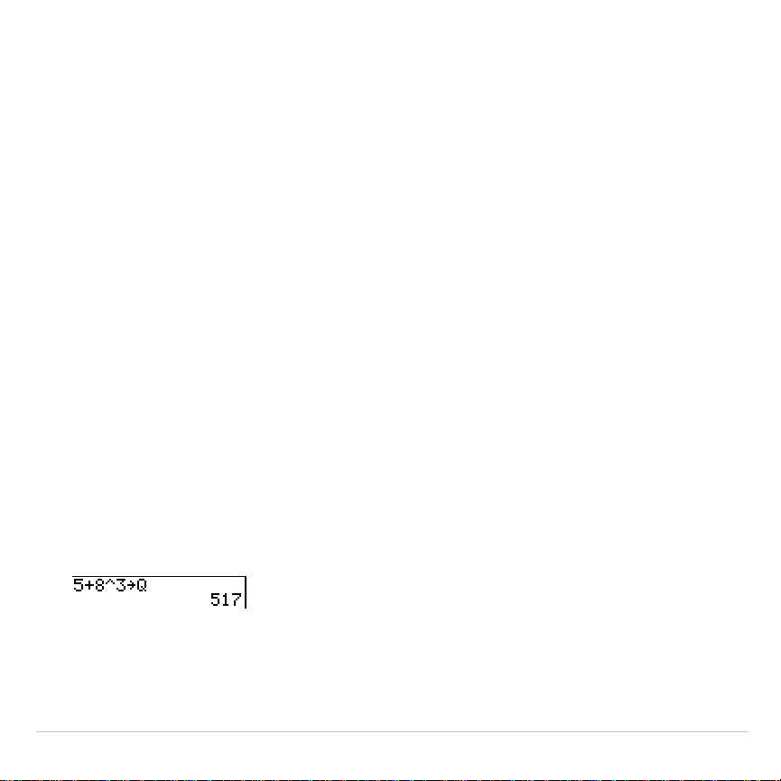
0
¿
ƒ
N
Í
ƒ
N
Ã
1
¿
ƒ
N
ƒ
ã
:
ä
ƒ
N
¡
Í
Í
Í
Multiple Entry Values on a Line
To store to
ENTRY
two or more expressions or instructions, separate each
expression or instruction with a colon, then press
Í
. All expressions
and instructions separated by colons are stored in
ENTRY
.
When you press
y
[
, all the expressions and instructions separated
by colons are pasted to the current cursor location. You can edit any of the
entries, and then execute all of them when you press
Í
.
TI-83 Plus Operating the TI-83 Plus Silver Edition 36
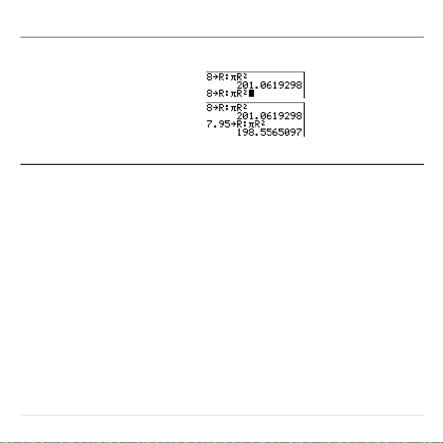
For the equation A=
p
r
2
, use trial and error to find the radius of a circle that covers 200
square centimeters. Use 8 as your first guess.
8
¿
ƒ
R
ƒ
[
:
]
y
B
ƒ
R
¡
Í
y
[
y
|
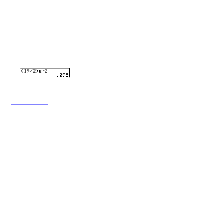
7
y
6
Ë
95
Í
Continue until the answer is as accurate as you want.
Clearing ENTRY
Clear Entries
(Chapter 18) clears all data that the TI-83 Plus is holding in
the
ENTRY
storage area.
Using Ans in an Expression
When an expression is evaluated successfully from the home screen or
from a program, the TI-83 Plus stores the answer to a storage area
called
Ans
(last answer).
Ans
may be a real or complex number, a list, a
matrix, or a string. When you turn off the TI-83 Plus, the value in
Ans
is
retained in memory.
TI-83 Plus Operating the TI-83 Plus Silver Edition 37
You can use the variable
Ans
to represent the last answer in most places.
Press
y
Z
to copy the variable name
Ans
to the cursor location. When
the expression is evaluated, the TI-83 Plus uses the value of
Ans
in the
calculation.
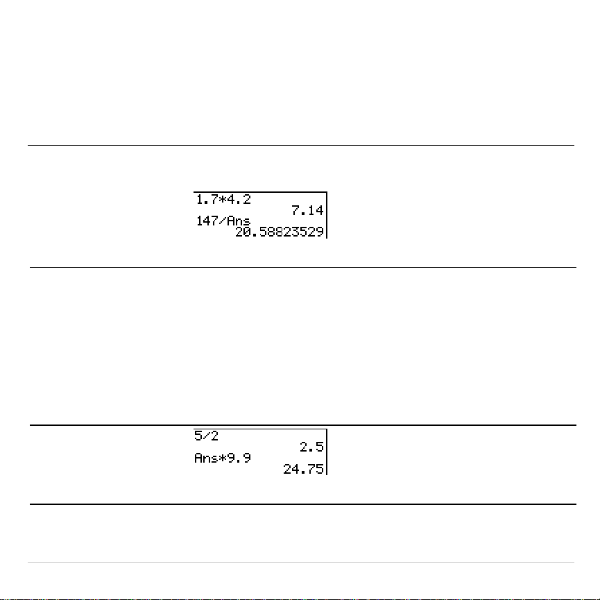
Calculate the area of a garden plot 1.7 meters by 4.2 meters. Then calculate the yield
per square meter if the plot produces a total of 147 tomatoes.
1
Ë
7
¯
4
Ë
2
Í
147
¥
y
Z
Í
Continuing an Expression
You can use
Ans
as the first entry in the next expression without entering
the value again or pressing
y
Z
. On a blank line on the home
screen, enter the function. The TI-83 Plus pastes the variable name
Ans
to the screen, then the function.
5
¥
2
Í
¯
9
Ë
9
Í
TI-83 Plus Operating the TI-83 Plus Silver Edition 38
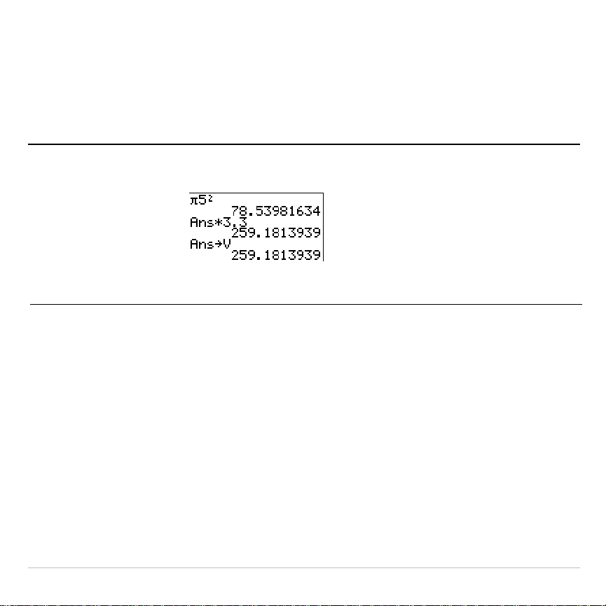
Storing Answers
To store an answer, store
Ans
to a variable before you evaluate another
expression.
Calculate the area of a circle of radius 5 meters. Next, calculate the volume of a cylinder
of radius 5 meters and height 3.3 meters, and then store the result in the variable V.
y
B
5
¡
Í
¯
3
Ë
3
Í
¿
ƒ
V
Í
TI-83 Plus Operating the TI-83 Plus Silver Edition 39
TI-83 Plus Menus
Using a TI-83 Plus Menu
You can access most TI-83 Plus operations using menus. When you
press a key or key combination to display a menu, one or more menu
names appear on the top line of the screen.
•
The menu name on the left side of the top line is highlighted. Up to
seven items in that menu are displayed, beginning with item
1
, which
also is highlighted.
•
A number or letter identifies each menu item’s place in the menu. The
order is
1
through
9
, then
0
, then
A
,
B
,
C
, and so on. The
LIST NAMES
,
PRGM EXEC
, and
PRGM EDIT
menus only label items
1
through
9
and
0
.
•
When the menu continues beyond the displayed items, a down arrow
(
$
) replaces the colon next to the last displayed item.
•
When a menu item ends in an ellipsis (...), the item displays a
secondary menu or editor when you select it.
•
When an asterisk (*) appears to the left of a menu item, that item is
stored in user data archive (Chapter 18).
TI-83 Plus Operating the TI-83 Plus Silver Edition 40
To display any other menu listed on the top line, press
~
or
|
until that
menu name is highlighted. The cursor location within the initial menu is
irrelevant. The menu is displayed with the cursor on the first item.
Note:
The Menu Map in Appendix A shows each menu, each operation under
each menu, and the key or key combination you press to display each menu.
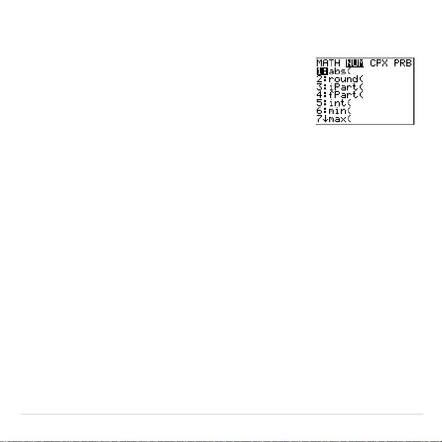
Displaying a Menu
While using your TI-83 Plus, you often will need
to access items from its menus.
When you press a key that displays a menu, that
menu temporarily replaces the screen where you
are working. For example, when you press
,
the
MATH
menu is displayed as a full screen.
After you select an item from a menu, the screen
where you are working usually is displayed again.
TI-83 Plus Operating the TI-83 Plus Silver Edition 41
Moving from One Menu to Another
Some keys access more than one menu. When
you press such a key, the names of all accessible
menus are displayed on the top line. When you
highlight a menu name, the items in that menu are
displayed. Press
~
and
|
to highlight each menu
name.
Scrolling a Menu
To scroll down the menu items, press
†
. To scroll up the menu items,
press
}
.
To page down six menu items at a time, press
ƒ
†
. To page up six
menu items at a time, press
ƒ
}
. The green arrows on the
calculator, between
†
and
}
, are the page-down and page-up symbols.
To wrap to the last menu item directly from the first menu item, press
}
.
To wrap to the first menu item directly from the last menu item, press
†
.
Selecting an Item from a Menu
You can select an item from a menu in either of two ways.
TI-83 Plus Operating the TI-83 Plus Silver Edition 42
•
Press the number or letter of the item you want
to select. The cursor can be anywhere on the
menu, and the item you select need not be
displayed on the screen.
•
Press
†
or
}
to move the cursor to the item
you want, and then press
Í
.
After you select an item from a menu, the
TI-83 Plus typically displays the previous screen.
Note:
On the
LIST NAMES
,
PRGM EXEC
, and
PRGM EDIT
menus, only items
1
through
9
and
0
are labeled in such a way that you can select them by pressing
the appropriate number key. To move the cursor to the first item beginning with
any alpha character or
q
, press the key combination for that alpha character or
q
. If no items begin with that character, the cursor moves beyond it to the next
item.
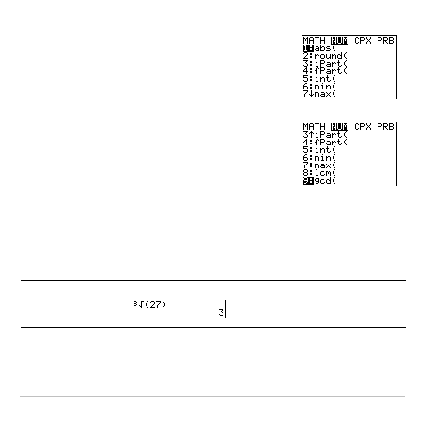
Calculate
3
‡
27.
†
†
†
Í
27
¤
Í

TI-83 Plus Operating the TI-83 Plus Silver Edition 43
Leaving a Menu without Making a Selection
You can leave a menu without making a selection in any of four ways.
•
Press
y
5
to return to the home screen.
•
Press
‘
to return to the previous screen.
•
Press a key or key combination for a different menu, such as
or
y
9
.
•
Press a key or key combination for a different screen, such as
o
or
y
0
.
TI-83 Plus Operating the TI-83 Plus Silver Edition 44
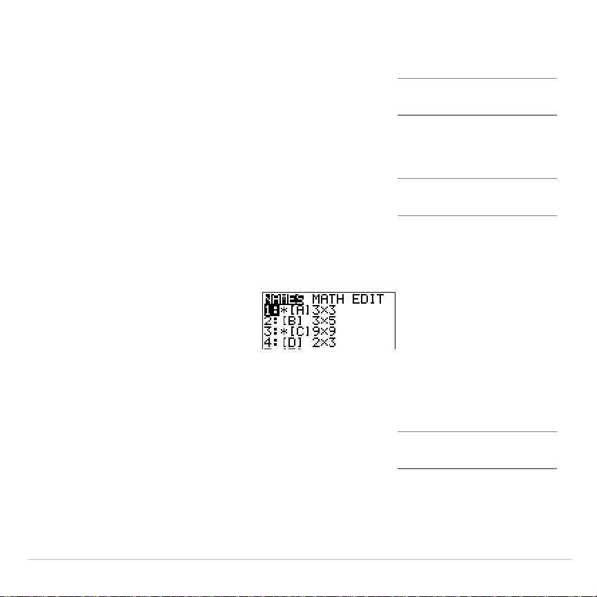
VARS and VARS Y
.
VARS Menus
VARS Menu
You can enter the names of functions and system variables in an
expression or store to them directly.
To display the
VARS
menu, press
. All
VARS
menu items display
secondary menus, which show the names of the system variables.
1:Window
,
2:Zoom
, and
5:Statistics
each access more than one
secondary menu.
VARS Y-VARS
1: Window
...
X/Y
,
T/
q
, and
U/V/W
variables
2: Zoom
...
ZX/ZY
,
ZT/Z
q
, and
ZU
variables
3: GDB
...
Graph database
variables
4: Picture
...
Picture
variables
5: Statistics
...
XY
,
G
,
EQ
,
TEST
, and
PTS
variables
6: Table
...
TABLE
variables
7: String
...
String
variables
TI-83 Plus Operating the TI-83 Plus Silver Edition 45
Selecting a Variable from the VARS Menu or VARS Y
.
VARS Menu
To display the
VARS Y
.
VARS
menu, press
~
.
1:Function
,
2:Parametric
, and
3:Polar
display secondary menus of the
Y=
function
variables.
VARS Y-VARS
1: Function
...
Y
n
functions
2: Parametric
...
X
n
T
,
Y
n
T
functions
3: Polar
...
r
n
functions
4: On/Off
...
Lets you select/deselect functions
Note: The sequence variables (
u
,
v
,
w
) are located on the keyboard as the
second functions of
¬
,
−
, and
®
.
To select a variable from the
VARS
or
VARS Y
.
VARS
menu, follow these
steps.
1. Display the
VARS
or
VARS Y
.
VARS
menu.
•
Press
to display the
VARS
menu.
•
Press
~
to display the
VARS Y
.
VARS
menu.
2. Select the type of variable, such as
2:Zoom
from the
VARS
menu or
3:Polar
from the
VARS Y
.
VARS
menu. A secondary menu is displayed.

TI-83 Plus Operating the TI-83 Plus Silver Edition 46
3. If you selected
1:Window
,
2:Zoom
, or
5:Statistics
from the
VARS
menu,
you can press
~
or
|
to display other secondary menus.
4. Select a variable name from the menu. It is pasted to the cursor
location.

TI-83 Plus Operating the TI-83 Plus Silver Edition 47
Equation Operating System (EOS)
Order of Evaluation
The Equation Operating System (EOS) defines the order in which
functions in expressions are entered and evaluated on the TI-83 Plus.
EOS lets you enter numbers and functions in a simple, straightforward
sequence.
EOS evaluates the functions in an expression in this order.
Order Number Function
1
Functions that precede the argument, such as
‡
(
,
sin(
, or
log(
2
Functions that are entered after the argument, such as
2
,
M
1
,
!
,
¡
,
r
, and conversions
3
Powers and roots, such as
2^5
or
5
x
‡
32
4
Permutations (
nPr
) and combinations (
nCr
)
5
Multiplication, implied multiplication, and division
6
Addition and subtraction
7
Relational functions, such as
>
or
8
Logic operator
and
9
Logic operators
or
and
xor
TI-83 Plus Operating the TI-83 Plus Silver Edition 48
Note:
Within a priority level, EOS evaluates functions from left to right.
Calculations within parentheses are evaluated first.
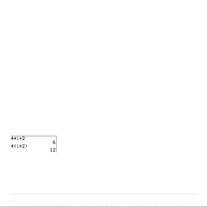
Implied Multiplication
The TI-83 Plus recognizes implied multiplication, so you need not press
¯
to express multiplication in all cases. For example, the TI-83 Plus
interprets
2
p
,
4sin(46)
,
5(1+2)
, and
(2
ä
5)7
as implied multiplication.
Note:
TI-83 Plus implied multiplication rules, although like theTI
.
83, differ from
those of the TI
.
82. For example, the TI-83 Plus evaluates
1
à
2X
as
(1
à
2)
ä
X
,
while the TI
.
82 evaluates
1
à
2X
as
1/(2
ä
X)
(Chapter 2).
Parentheses
All calculations inside a pair of parentheses are completed first. For
example, in the expression
4(1+2)
, EOS first evaluates the portion inside
the parentheses,
1+2
, and then multiplies the answer,
3
, by
4
.
You can omit the close parenthesis (
)
) at the end of an expression. All
open parenthetical elements are closed automatically at the end of an
expression. This is also true for open parenthetical elements that
precede the store or display-conversion instructions.
TI-83 Plus Operating the TI-83 Plus Silver Edition 49
Note:
An open parenthesis following a list name, matrix name, or
Y=
function
name does not indicate implied multiplication. It specifies elements in the list
(Chapter 11) or matrix (Chapter 10) and specifies a value for which to solve the
Y=
function.
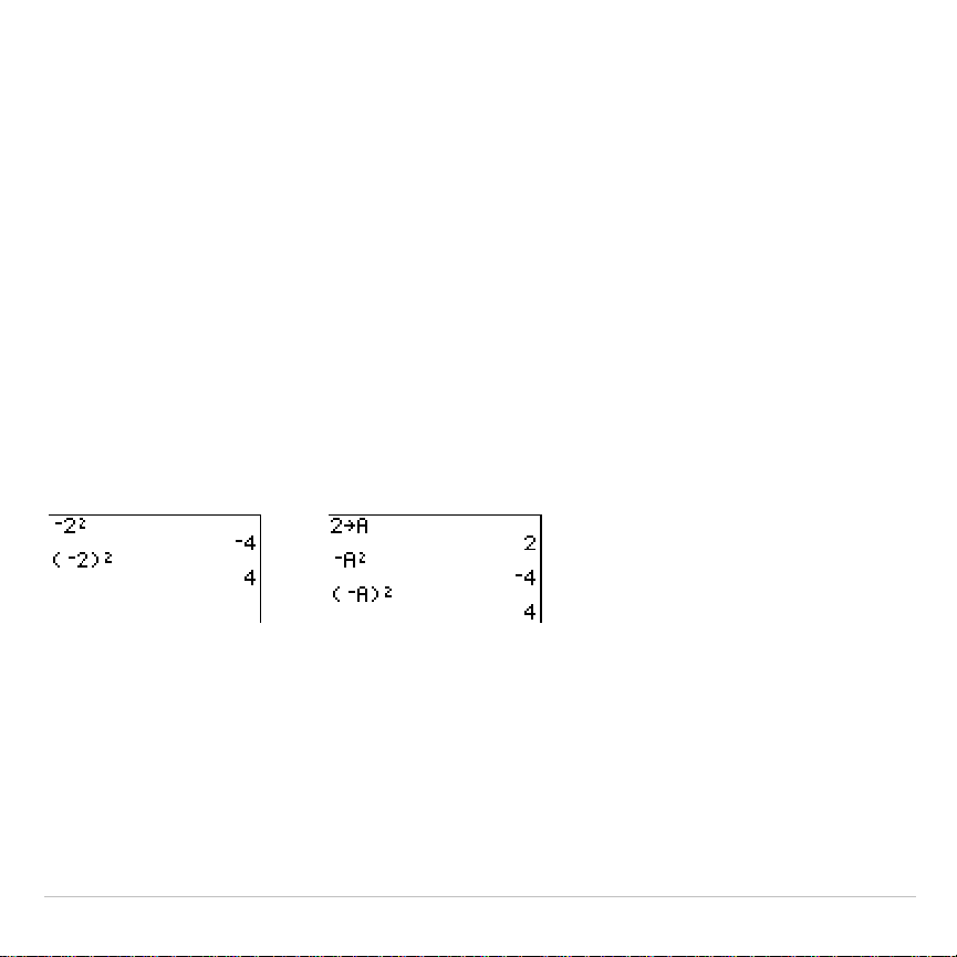
Negation
To enter a negative number, use the negation key. Press
Ì
and then
enter the number. On the TI-83 Plus, negation is in the third level in the
EOS hierarchy. Functions in the first level, such as squaring, are
evaluated before negation.
For example,
M
X
2
, evaluates to a negative number (or 0). Use
parentheses to square a negative number.
Note:
Use the
¹
key for subtraction and the
Ì
key for negation. If you press
¹
to enter a negative number, as in
9
¯
¹
7
, or if you press
Ì
to indicate
subtraction, as in
9
Ì
7
, an error occurs. If you press
ƒ
A
Ì
ƒ
B
, it is
interpreted as implied multiplication (
A
ä
M
B
).

TI-83 Plus Operating the TI-83 Plus Silver Edition 50
Special Features of the TI-83 Plus
Flash – Electronic Upgradability
The TI-83 Plus uses Flash
technology, which lets you
upgrade to future software
versions without buying a new
calculator.
For details, refer to:
Chapter 19
As new functionality becomes available, you can electronically upgrade
your TI-83 Plus from the Internet. Future software versions include
maintenance upgrades that will be released free of charge, as well as
new applications and major software upgrades that will be available for
purchase from the TI web site:
education.ti.com
1.56 Megabytes (M) of Available Memory
1.56 M of available memory are built into the
TI-83 Plus. About 24 kilobytes (K) of RAM
(random access memory) are available for you
to compute and store functions, programs, and
data.
For details, refer to:
Chapter 18
About 1.54 M of user data archive allow you to store data, programs,
applications, or any other variables to a safe location where they cannot

TI-83 Plus Operating the TI-83 Plus Silver Edition 51
be edited or deleted inadvertently. You can also free up RAM by
archiving variables to user data
Applications
Applications can be installed to customize the
TI-83 Plus to your classroom needs. The big
1.54 M archive space lets you store up to 94
applications at one time. Applications can also
be stored on a computer for later use or linked
unit-to-unit.
For details, refer to:
Chapter 18
Archiving
You can store variables in the TI-83 Plus user
data archive, a protected area of memory
separate from RAM. The user data archive lets
you:
For details, refer to:
Chapter 18
•
Store data, programs, applications or any other variables to a safe
location where they cannot be edited or deleted inadvertently.
•
Create additional free RAM by archiving variables.
By archiving variables that do not need to be edited frequently, you can
free up RAM for applications that may require additional memory.

TI-83 Plus Operating the TI-83 Plus Silver Edition 52
Calculator-Based Laboratory
é
(CBL 2
é
, CBL
é
) and
Calculator-Based Ranger
é
(CBR
é
)
The TI-83 Plus comes with the CBL/CBR
application already installed. When coupled
with the (optional) CBL 2/CBL or CBR
accessories, you can use the TI-83 Plus to
analyze real world data.
For details, refer to:
Chapter 14
CBL 2/CBL and CBR let you explore mathematical and scientific
relationships among distance, velocity, acceleration, and time using data
collected from activities you perform.
CBL 2/CBL and CBR differ in that CBL 2/CBL allows you to collect data
using several different probes analyzing temperature, light, voltage, or
sonic (motion) data. CBR collects data using a built-in Sonic probe.
CBL 2/CBL and CBR accessories can be linked together to collect more
than one type of data at the same time. You can find more information
on
CBL 2/CBL and CBR
in their user manuals.

TI-83 Plus Operating the TI-83 Plus Silver Edition 53
Other TI-83 Plus Features
Getting Started has introduced you to basic TI-83 Plus operations. This
guidebook covers the other features and capabilities of the TI-83 Plus in
greater detail.
Graphing
You can store, graph, and analyze up to 10
functions, up to six parametric functions, up to
six polar functions, and up to three sequences.
You can use
DRAW
instructions to annotate
graphs.
For graphing details,
refer to:
Chapters 3, 4, 5, 6, 8
The graphing chapters appear in this order:
Function
,
Parametric
,
Polar
,
Sequence
, and
DRAW
.
Sequences
You can generate sequences and graph them
over time. Or, you can graph them as web plots
or as phase plots.
For details, refer to:
Chapter 6

TI-83 Plus Operating the TI-83 Plus Silver Edition 54
Tables
You can create function evaluation tables to
analyze many functions simultaneously.
For details, refer to:
Chapter 7
Split Screen
You can split the screen horizontally to display
both a graph and a related editor (such as the
Y=
editor), the table, the stat list editor, or the
home screen. Also, you can split the screen
vertically to display a graph and its table
simultaneously.
For details, refer to:
Chapter 9
Matrices
You can enter and save up to 10 matrices and
perform standard matrix operations on them.
For details, refer to:
Chapter 10

TI-83 Plus Operating the TI-83 Plus Silver Edition 55
Lists
You can enter and save as many lists as
memory allows for use in statistical analyses.
You can attach formulas to lists for automatic
computation. You can use lists to evaluate
expressions at multiple values simultaneously
and to graph a family of curves.
For details, refer to:
Chapter 11
Statistics
You can perform one- and two-variable, list-
based statistical analyses, including logistic and
sine regression analysis. You can plot the data
as a histogram, xyLine, scatter plot, modified or
regular box-and-whisker plot, or normal
probability plot. You can define and store up to
three stat plot definitions.
For details, refer to:
Chapter 12
Inferential Statistics
You can perform 16 hypothesis tests and
confidence intervals and 15 distribution
functions. You can display hypothesis test
results graphically or numerically.
For details, refer to:
Chapter 13

TI-83 Plus Operating the TI-83 Plus Silver Edition 56
Applications
You can use such applications as Finance or
the CBL/CBR. With the Finance application you
can use time-value-of-money (
TVM
) functions to
analyze financial instruments such as annuities,
For details, refer to:
Chapter 14
loans, mortgages, leases, and savings. You can analyze the value of
money over equal time periods using cash flow functions. You can
amortize loans with the amortization functions. With the CBL/CBR
applications and CBL 2/CBL or CBR (optional) accessories, you can use
a variety of probes to collect real world data.
Your TI-83 Plus includes Flash applications in addition to the ones
mentioned above. Press
Œ
to see the complete list of applications
that came with your calculator.
Documentation for TI Flash applications is on the TI Resource CD. Visit
education.ti.com/calc/guides
for additional Flash application guidebooks.
CATALOG
The
CATALOG
is a convenient, alphabetical list of
all functions and instructions on the TI-83 Plus.
You can paste any function or instruction from
the
CATALOG
to the current cursor location.
For details, refer to:
Chapter 15
TI-83 Plus Operating the TI-83 Plus Silver Edition 57
Programming
You can enter and store programs that include
extensive control and input/output instructions.
For details, refer to:
Chapter 16
Archiving
Archiving allows you to store data, programs, or
other variables to user data archive where they
cannot be edited or deleted inadvertently.
Archiving also allows you to free up RAM for
variables that may require additional memory.
For details, refer to:
Chapter 16
Archived variables are
indicated by asterisks (*) to
the left of the variable
names.
Communication Link
The TI-83 Plus has a port to connect and
communicate with another TI-83 Plus, a
TI
-
83 Plus, a TI
.
83, a TI
-
82, a TI
-
73,
CBL 2/CBL, or a CBR System.
For details, refer to:
Chapter 19

TI-83 Plus Operating the TI-83 Plus Silver Edition 58
With the
TI™ Connect
or
TI-GRAPH LINK™
software and
a TI-GRAPH LINK
cable, you can also link the TI-83 Plus to a personal computer.
As future software upgrades become available on the TI web site, you
can download the software to your PC and then use the
TI Connect
or
TI-GRAPH LINK
software and a
TI-GRAPH LINK
cable to upgrade your
TI-83 Plus.
TI-83 Plus Operating the TI-83 Plus Silver Edition 59
Error Conditions
Diagnosing an Error
The TI-83 Plus detects errors while performing these tasks.
•
Evaluating an expression
•
Executing an instruction
•
Plotting a graph
•
Storing a value
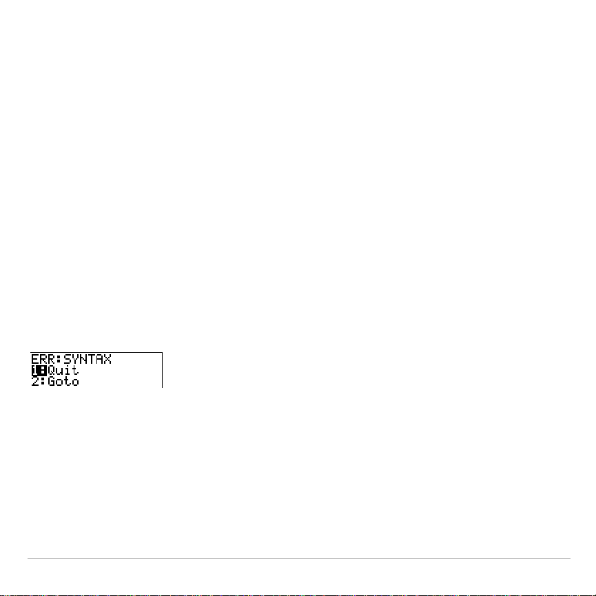
When the TI-83 Plus detects an error, it returns an error message as a
menu title, such as
ERR:SYNTAX
or
ERR:DOMAIN
. Appendix B describes
each error type and possible reasons for the error.
•
If you select
1:Quit
(or press
y
5
or
‘
), then the home
screen is displayed.
•
If you select
2:Goto
, then the previous screen is displayed with the
cursor at or near the error location.
Note: If a syntax error occurs in the contents of a
Y=
function during program
execution, then the
Goto
option returns to the
Y=
editor, not to the program.

TI-83 Plus Operating the TI-83 Plus Silver Edition 60
Correcting an Error
To correct an error, follow these steps.
1. Note the error type (
ERR:
error type
).
2. Select
2:Goto
, if it is available. The previous screen is displayed with
the cursor at or near the error location.
3. Determine the error. If you cannot recognize the error, refer to
Appendix B.
4. Correct the expression.
TI-83 Plus Math, Angle, and Test Operations 61
Chapter 2:
Math, Angle, and Test Operations
Getting Started: Coin Flip
Getting Started is a fast-paced introduction. Read the chapter for details.
Suppose you want to model flipping a fair coin 10 times. You want to track how
many of those 10 coin flips result in heads. You want to perform this simulation
40 times. With a fair coin, the probability of a coin flip resulting in heads is 0.5
and the probability of a coin flip resulting in tails is 0.5.
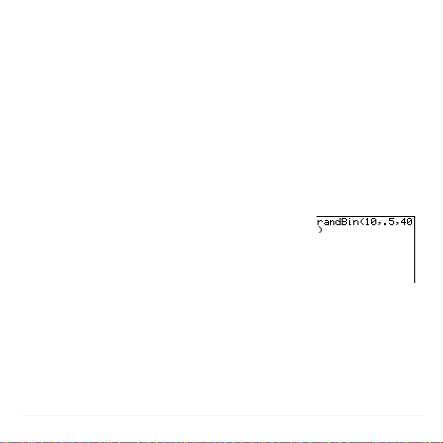
1. Begin on the home screen. Press
|
to
display the
MATH PRB
menu. Press
7
to select
7:randBin(
(random Binomial).
randBin(
is pasted
to the home screen. Press
10
to enter the
number of coin flips. Press
¢
. Press
Ë
5
to
enter the probability of heads. Press
¢
. Press
40
to enter the number of simulations. Press
¤
.
TI-83 Plus Math, Angle, and Test Operations 62
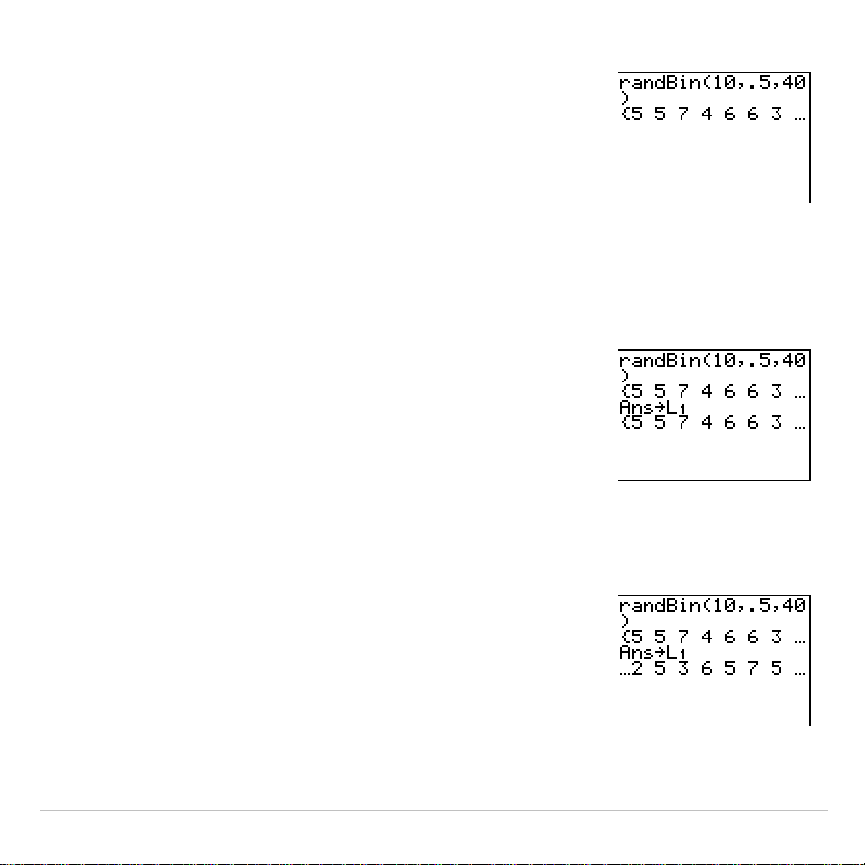
2. Press
Í
to evaluate the expression. A list of
40 elements is generated with the first 7
displayed. The list contains the count of heads
resulting from each set of 10 coin flips. The list
has 40 elements because this simulation was
performed 40 times. In this example, the coin
came up heads five times in the first set of 10
coin flips, five times in the second set of 10 coin
flips, and so on.
3. Press
~
or
|
to view the additional counts in
the list. Ellipses (
...
) indicate that the list
continues beyond the screen.
4. Press
¿
y
ã
L1ä
Í
to store the data to
the list name
L1
. You then can use the data for
another activity, such as plotting a histogram
(Chapter 12).
Note: Since
randBin(
generates random numbers,
your list elements may differ from those in the
example.
TI-83 Plus Math, Angle, and Test Operations 63
Keyboard Math Operations
Using Lists with Math Operations
Math operations that are valid for lists return a list calculated element by
element. If you use two lists in the same expression, they must be the
same length.
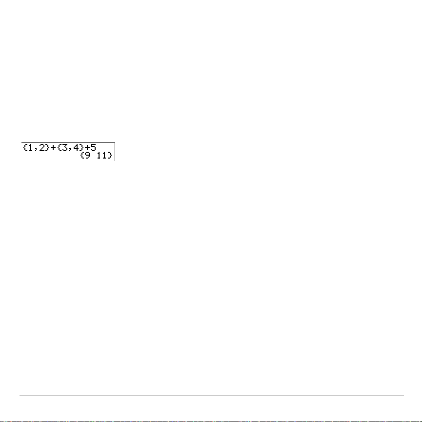
+ (Addition),
N
(Subtraction),
ä
(Multiplication),
à
(Division)
You can use
+
(addition,
Ã
),
N
(subtraction,
¹
),
ä
(multiplication,
¯
), and
à
(division,
¥
) with real and complex numbers, expressions, lists, and
matrices. You cannot use
à
with matrices.
valueA
+
valueB valueA
N
valueB
valueA
ä
valueB valueA
à
valueB
Trigonometric Functions
You can use the trigonometric (trig) functions (sine,
˜
; cosine,
™
;
and tangent,
š
) with real numbers, expressions, and lists. The current
angle mode setting affects interpretation. For example,
sin(30)
in
Radian
mode returns
L
.9880316241
; in
Degree
mode it returns
.5
.
TI-83 Plus Math, Angle, and Test Operations 64
sin(
value
) cos(
value
) tan(
value
)
You can use the inverse trig functions (arcsine,
y
?
; arccosine,
y
@
; and arctangent,
y
A
) with real numbers, expressions, and
lists. The current angle mode setting affects interpretation.
sin
L
1
(
value
) cos
L
1
(
value
) tan
L
1
(
value
)
Note: The trig functions do not operate on complex numbers.
^ (Power),
2
(Square),
‡
( (Square Root)
You can use
^
(power,
›
),
2
(square,
¡
), and
‡
(
(square root,
y
C
)
with real and complex numbers, expressions, lists, and matrices. You
cannot use
‡
(
with matrices.
value
^
power value
2
‡
(
value
)
L
1
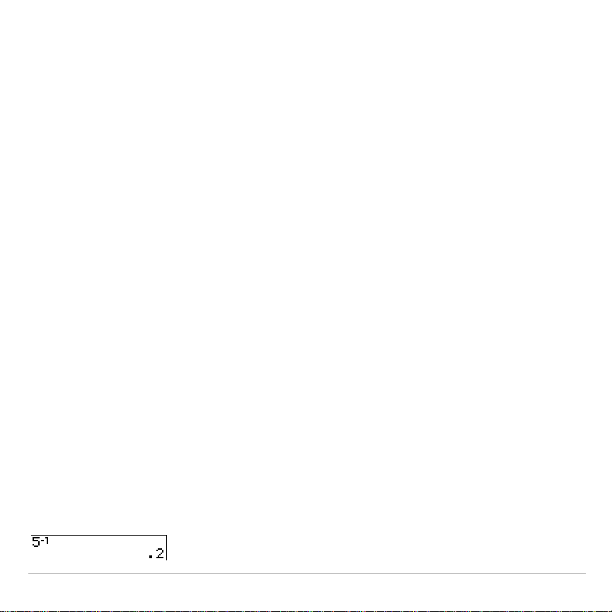
(Inverse)
You can use
L
1
(inverse,
œ
) with real and complex numbers,
expressions, lists, and matrices. The multiplicative inverse is equivalent
to the reciprocal, 1
à
x
.
value
L
1
TI-83 Plus Math, Angle, and Test Operations 65
log(, 10^(, ln(
You can use
log(
(logarithm,
«
),
10^(
(power of 10,
y
G
), and
ln(
(natural log,
µ
) with real or complex numbers, expressions, and lists.
log(
value
) 10^(
power
) ln(
value
)
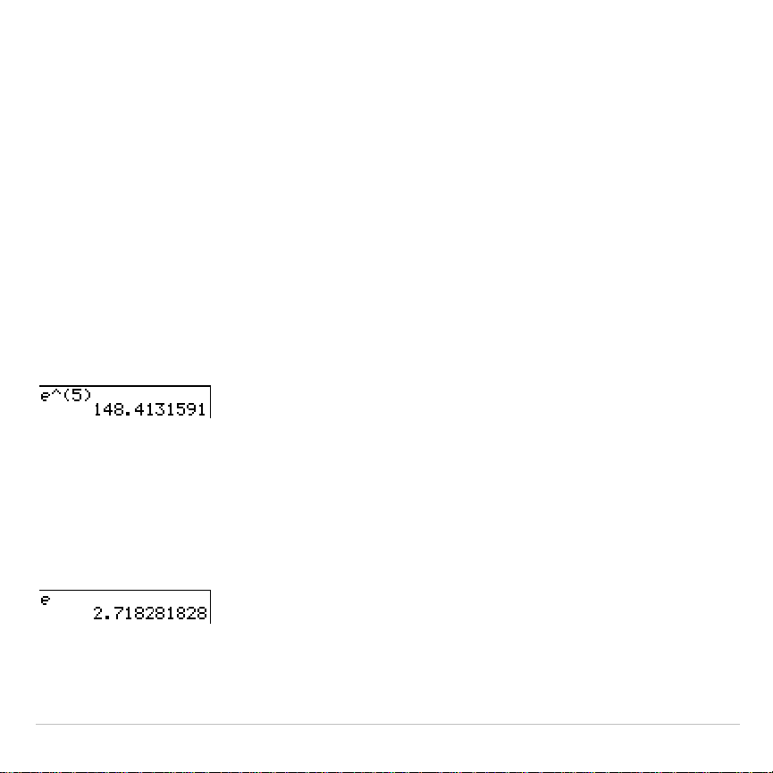
e^( (Exponential)
e^(
(exponential,
y
J
) returns the constant
e
raised to a power. You
can use
e^(
with real or complex numbers, expressions, and lists.
e^(
power
)
e (Constant)
e
(constant,
y
[
e
]) is stored as a constant on the TI-83 Plus. Press
y
[
e
] to copy
e
to the cursor location. In calculations, the TI-83 Plus
uses 2.718281828459 for
e
.
TI-83 Plus Math, Angle, and Test Operations 66
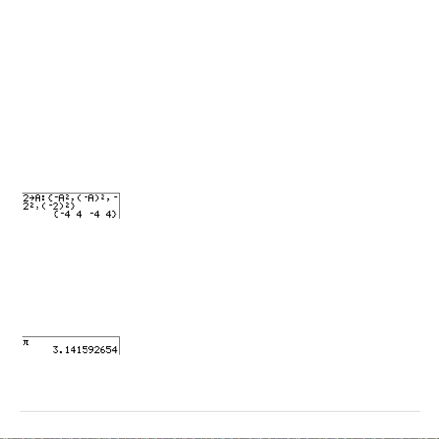
L
(Negation)
M
(negation,
Ì
) returns the negative of
value
. You can use
M
with real or
complex numbers, expressions, lists, and matrices.
M
value
EOS™ rules (Chapter 1) determine when negation is evaluated. For
example,
L
A
2
returns a negative number, because squaring is evaluated
before negation. Use parentheses to square a negated number, as in
(
L
A)
2
.
Note: On the TI-83 Plus, the negation symbol (
M
) is shorter and higher than the
subtraction sign (
N
), which is displayed when you press
¹
.
p
(Pi)
p
(Pi,
y
B
) is stored as a constant in the TI-83 Plus. In calculations,
the TI-83 Plus uses 3.1415926535898 for
p
.

TI-83 Plus Math, Angle, and Test Operations 67
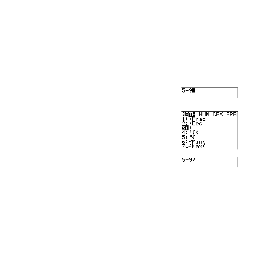
MATH Operations
MATH Menu
To display the
MATH
menu, press
.
MATH NUM CPX PRB
1:
4
Frac
Displays the answer as a fraction.
2:
4
Dec
Displays the answer as a decimal.
3:
3
Calculates the cube.
4:
3
‡
(
Calculates the cube root.
5:
x
‡
Calculates the
x
th
root.
6: fMin(
Finds the minimum of a function.
7: fMax(
Finds the maximum of a function.
8: nDeriv(
Computes the numerical derivative.
9: fnInt(
Computes the function integral.
0: Solver
...
Displays the equation solver.
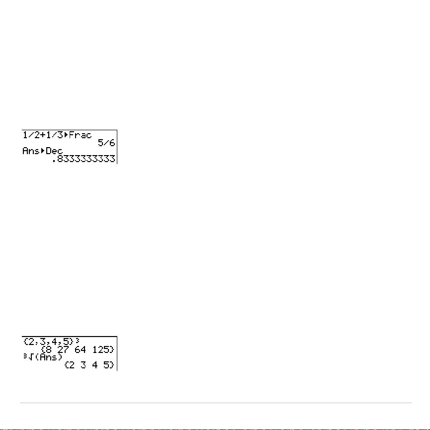
4
Frac,
4
Dec
4
Frac
(display as a fraction) displays an answer as its rational equivalent.
You can use
4
Frac
with real or complex numbers, expressions, lists, and
matrices. If the answer cannot be simplified or the resulting denominator
is more than three digits, the decimal equivalent is returned. You can
only use
4
Frac
following
value
.
TI-83 Plus Math, Angle, and Test Operations 68
value
4
Frac
4
Dec
(display as a decimal) displays an answer in decimal form. You can
use
4
Dec
with real or complex numbers, expressions, lists, and matrices.
You can only use
4
Dec
following
value
.
value
4
Dec
3
(Cube),
3
‡
( (Cube Root)
3
(cube) returns the cube of
value
. You can use
3
with real or complex
numbers, expressions, lists, and square matrices.
value
3
3
‡
(
(cube root) returns the cube root of
value
. You can use
3
‡
(
with real or
complex numbers, expressions, and lists.
3
‡
(
value
)
TI-83 Plus Math, Angle, and Test Operations 69
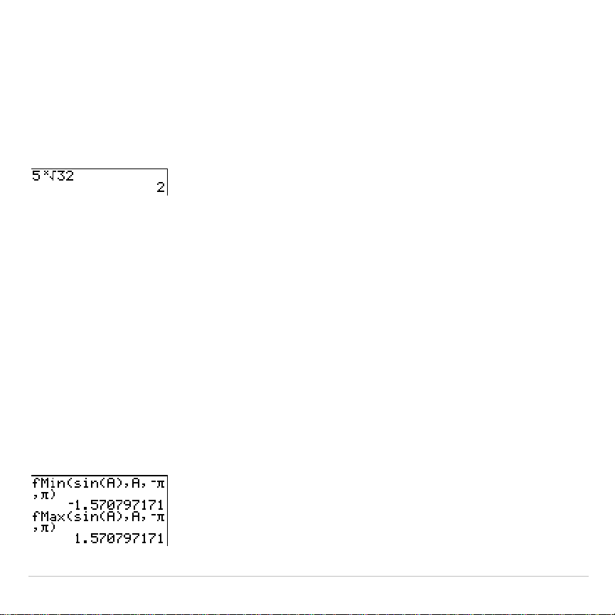
x
‡
(Root)
x
‡
(
x
th
root) returns the
x
th
root
of
value
. You can use
x
‡
with real or
complex numbers, expressions, and lists.
x
th
root
x
‡
value
fMin(, fMax(
fMin(
(function minimum) and
fMax(
(function maximum) return the value
at which the local minimum or local maximum value of
expression
with
respect to
variable
occurs, between
lower
and
upper
values for
variable
.
fMin(
and
fMax(
are not valid in
expression
. The accuracy is controlled by
tolerance
(if not specified, the default is 1
â
L
5).
fMin(
expression
,
variable
,
lower
,
upper
[
,
tolerance
]
)
fMax(
expression
,
variable
,
lower
,
upper
[
,
tolerance
]
)
Note: In this guidebook, optional arguments and the commas that accompany
them are enclosed in brackets ([ ]).
TI-83 Plus Math, Angle, and Test Operations 70
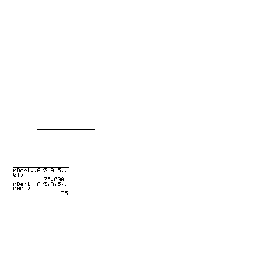
nDeriv(
nDeriv(
(numerical derivative) returns an approximate derivative of
expression
with respect to
variable
, given the
value
at which to calculate the
derivative and
H
(if not specified, the default is 1
â
L
3).
nDeriv(
is valid only
for real numbers.
nDeriv(
expression
,
variable
,
value
[
,
H
]
)
nDeriv(
uses the symmetric difference quotient method, which
approximates the numerical derivative value as the slope of the secant
line through these points.
ε
εε
2
)(()(
)('
−−+
=
xfxf
xf
As
H
becomes smaller, the approximation usually becomes more
accurate.
You can use
nDeriv(
once in
expression
. Because of the method used to
calculate
nDeriv(
, the TI-83 Plus can return a false derivative value at a
nondifferentiable point.
TI-83 Plus Math, Angle, and Test Operations 71
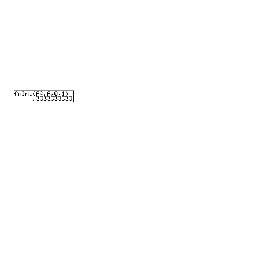
fnInt(
fnInt(
(function integral) returns the numerical integral (Gauss-Kronrod
method) of
expression
with respect to
variable
, given
lower
limit,
upper
limit,
and a
tolerance
(if not specified, the default is 1
â
L
5).
fnInt(
is valid only for
real numbers.
fnInt(
expression
,
variable
,
lower
,
upper
[
,
tolerance
]
)
Tip: To speed the drawing of integration graphs (when
fnInt(
is used in a Y=
equation), increase the value of the
Xres
window variable before you press
s
.

TI-83 Plus Math, Angle, and Test Operations 72
Using the Equation Solver
Solver
Solver
displays the equation solver, in which you can solve for any
variable in an equation. The equation is assumed to be equal to zero.
Solver
is valid only for real numbers.
When you select
Solver
, one of two screens is displayed.
•
The equation editor (see step 1 picture below) is displayed when the
equation variable
eqn
is empty.
•
The interactive solver editor is displayed when an equation is stored
in
eqn
.
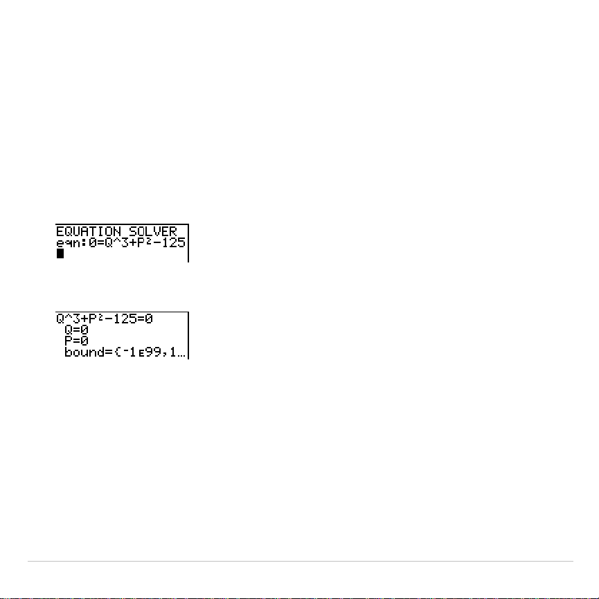
Entering an Expression in the Equation Solver
To enter an expression in the equation solver, assuming that the variable
eqn
is empty, follow these steps.
1. Select
0:Solver
from the
MATH
menu to display the equation editor.
2. Enter the expression in any of three ways.
TI-83 Plus Math, Angle, and Test Operations 73
•
Enter the expression directly into the equation solver.
•
Paste a
Y=
variable name from the
VARS Y
.
VARS
menu to the
equation solver.
•
Press
y
K
, paste a
Y=
variable name from the
VARS Y
.
VARS
menu, and press
Í
. The expression is pasted to the equation
solver.
The expression is stored to the variable
eqn
as you enter it.
3. Press
Í
or
†
. The interactive solver editor is displayed.
•
The equation stored in
eqn
is set equal to zero and displayed on
the top line.
•
Variables in the equation are listed in the order in which they
appear in the equation. Any values stored to the listed variables
also are displayed.
•
The default lower and upper bounds appear in the last line of the
editor (
bound={
L
1
å
99,1
å
99}
).
TI-83 Plus Math, Angle, and Test Operations 74
•
A
$
is displayed in the first column of the bottom line if the editor
continues beyond the screen.
Tip:
To use the solver to solve an equation such as
K=.5MV
2
, enter
eqn:0=K
N
.5MV
2
in the equation editor.
Entering and Editing Variable Values
When you enter or edit a value for a variable in the interactive solver
editor, the new value is stored in memory to that variable.
You can enter an expression for a variable value. It is evaluated when
you move to the next variable. Expressions must resolve to real numbers
at each step during the iteration.
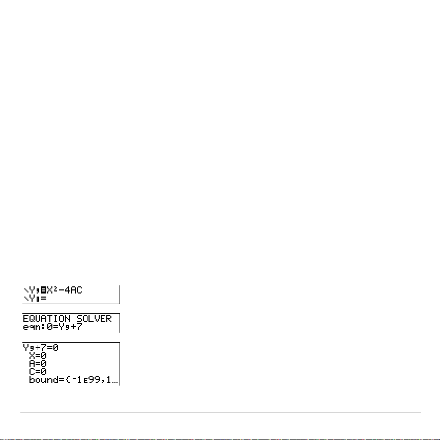
You can store equations to any
VARS Y
.
VARS
variables, such as
Y
1
or
r
6
,
and then reference the variables in the equation. The interactive solver
editor displays all variables of all
Y=
functions referenced in the equation.
TI-83 Plus Math, Angle, and Test Operations 75
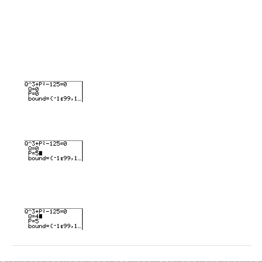
Solving for a Variable in the Equation Solver
To solve for a variable using the equation solver after an equation has
been stored to
eqn
, follow these steps.
1. Select
0:Solver
from the
MATH
menu to display the interactive solver
editor, if not already displayed.
2. Enter or edit the value of each known variable. All variables, except
the unknown variable, must contain a value. To move the cursor to
the next variable, press
Í
or
†
.
3. Enter an initial guess for the variable for which you are solving. This
is optional, but it may help find the solution more quickly. Also, for
equations with multiple roots, the TI-83 Plus will attempt to display
the solution that is closest to your guess.
TI-83 Plus Math, Angle, and Test Operations 76
The default guess is calculated as
(upper+lower)
2
.
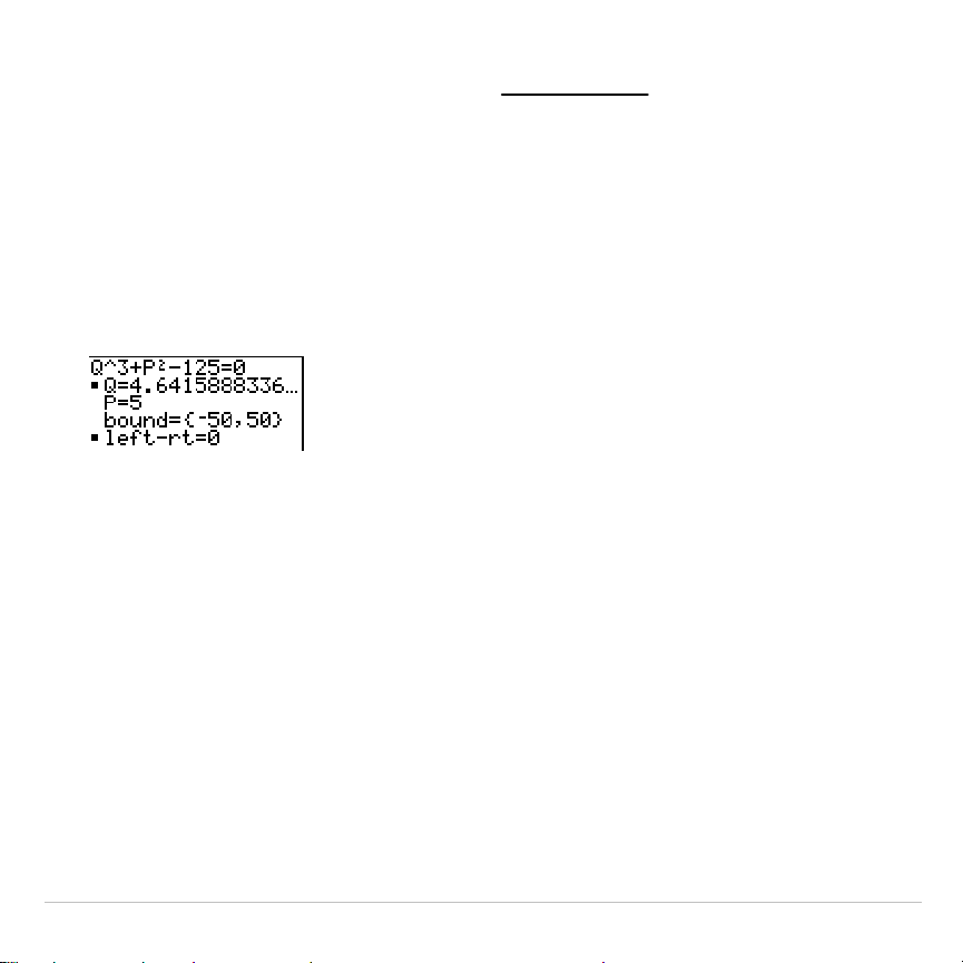
4. Edit
bound={
lower
,
upper
}
.
lower
and
upper
are the bounds between which
the TI-83 Plus searches for a solution. This is optional, but it may help
find the solution more quickly. The default is
bound={
L
1
å
99,1
å
99}
.
5. Move the cursor to the variable for which you want to solve and press
ƒ
\
(above the
Í
key).
•
The solution is displayed next to the variable for which you solved.
A solid square in the first column marks the variable for which you
solved and indicates that the equation is balanced. An ellipsis
shows that the value continues beyond the screen.
Note: When a number continues beyond the screen, be sure to press
~
to scroll to the end of the number to see whether it ends with a negative
or positive exponent. A very small number may appear to be a large
number until you scroll right to see the exponent.
•
The values of the variables are updated in memory.
TI-83 Plus Math, Angle, and Test Operations 77
•
left
N
rt=
diff
is displayed in the last line of the editor.
diff
is the
difference between the left and right sides of the equation. A solid
square in the first column next to
left
N
rt=
indicates that the
equation has been evaluated at the new value of the variable for
which you solved.
Editing an Equation Stored to eqn
To edit or replace an equation stored to
eqn
when the interactive
equation solver is displayed, press
}
until the equation editor is
displayed. Then edit the equation.
Equations with Multiple Roots
Some equations have more than one solution. You can enter a new
initial guess or new bounds to look for additional solutions.
Further Solutions
After you solve for a variable, you can continue to explore solutions from
the interactive solver editor. Edit the values of one or more variables.
When you edit any variable value, the solid squares next to the previous
solution and
left
N
rt=
diff
disappear. Move the cursor to the variable for
which you now want to solve and press
ƒ
\
.
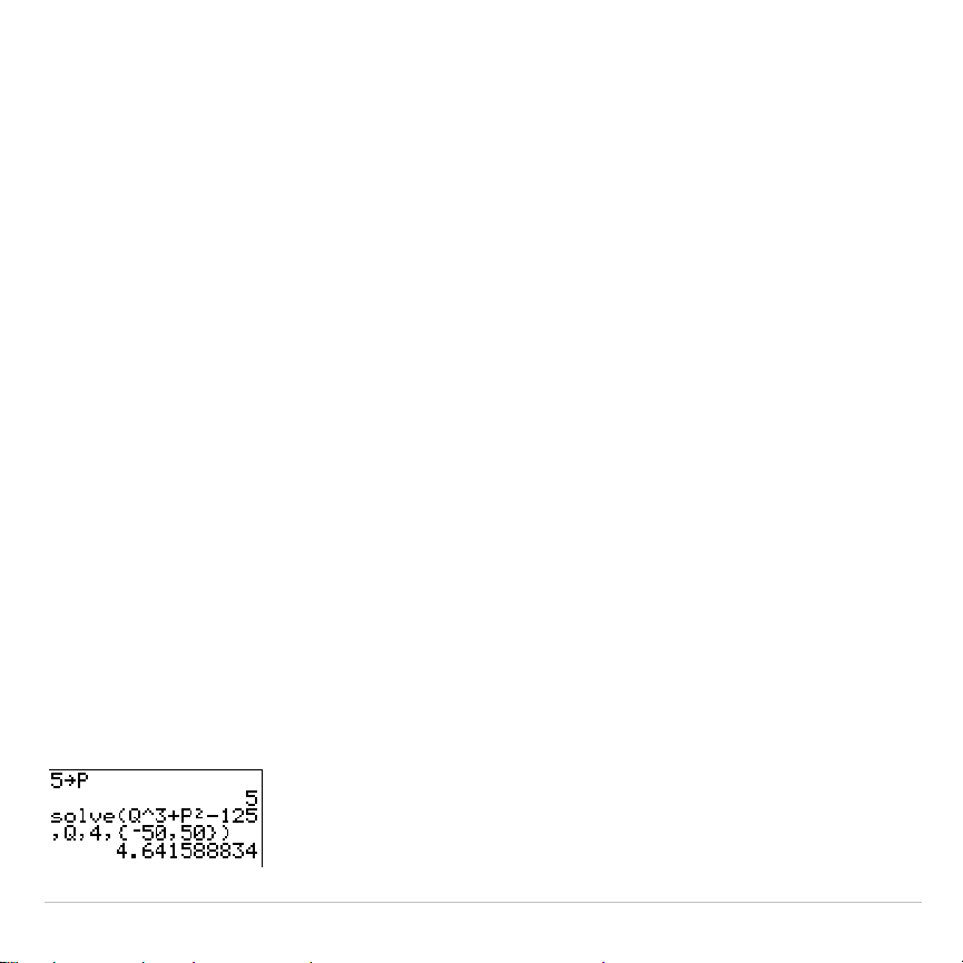
TI-83 Plus Math, Angle, and Test Operations 78
Controlling the Solution for Solver or solve(
The TI-83 Plus solves equations through an iterative process. To control
that process, enter bounds that are relatively close to the solution and
enter an initial guess within those bounds. This will help to find a solution
more quickly. Also, it will define which solution you want for equations
with multiple solutions.
Using solve( on the Home Screen or from a Program
The function
solve(
is available only from
CATALOG
or from within a
program. It returns a solution (root) of
expression
for
variable
, given an
initial
guess
, and
lower
and
upper
bounds within which the solution is
sought. The default for
lower
is
L
1
â
99. The default for
upper
is 1
â
99.
solve(
is valid only for real numbers.
solve(
expression
,
variable
,
guess
[
,{
lower
,
upper
}
]
)
expression
is assumed equal to zero. The value of
variable
will not be
updated in memory.
guess
may be a value or a list of two values. Values
must be stored for every variable in
expression
, except
variable
, before
expression
is evaluated.
lower
and
upper
must be entered in list format.
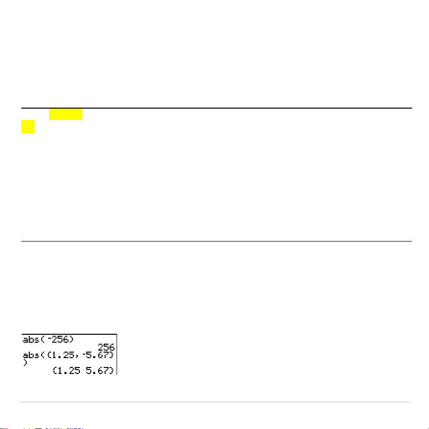
TI-83 Plus Math, Angle, and Test Operations 79
MATH NUM (Number) Operations
MATH NUM Menu
To display the
MATH NUM
menu, press
~
.
MATH NUM CPX PRB
1: abs(
Absolute value
2: round(
Round
3: iPart(
Integer part
4: fPart(
Fractional part
5: int(
Greatest integer
6: min(
Minimum value
7: max(
Maximum value
8: lcm(
Least common multiple
9: gcd(
Greatest common divisor
abs(
abs(
(absolute value) returns the absolute value of real or complex
(modulus) numbers, expressions, lists, and matrices.
abs(
value
)
Note:
abs(
is also available on the
MATH CPX
menu.
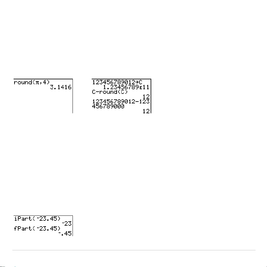
TI-83 Plus Math, Angle, and Test Operations 80
round(
round(
returns a number, expression, list, or matrix rounded to
#decimals
(
9). If
#decimals
is omitted,
value
is rounded to the digits that are
displayed, up to 10 digits.
round(
value
[
,
#decimals
]
)
iPart(, fPart(
iPart(
(integer part) returns the integer part or parts of real or complex
numbers, expressions, lists, and matrices.
iPart(
value
)
fPart(
(fractional part) returns the fractional part or parts of real or complex
numbers, expressions, lists, and matrices.
fPart(
value
)

TI-83 Plus Math, Angle, and Test Operations 81
int(
int(
(greatest integer) returns the largest integer
real or complex
numbers, expressions, lists, and matrices.
int(
value
)
Note: For a given
value
, the result of
int(
is the same as the result of
iPart(
for
nonnegative numbers and negative integers, but one integer less than the
result of
iPart(
for negative noninteger numbers.
min(, max(
min(
(minimum value) returns the smaller of
valueA
and
valueB
or the
smallest element in
list
. If
listA
and
listB
are compared,
min(
returns a list
of the smaller of each pair of elements. If
list
and
value
are compared,
min(
compares each element in
list
with
value
.
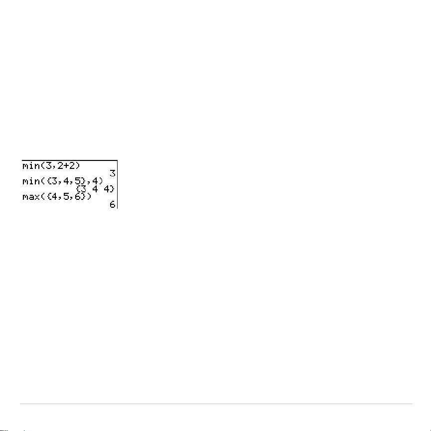
TI-83 Plus Math, Angle, and Test Operations 82
max(
(maximum value) returns the larger of
valueA
and
valueB
or the
largest element in
list
. If
listA
and
listB
are compared,
max(
returns a list of
the larger of each pair of elements. If
list
and
value
are compared,
max(
compares each element in
list
with
value
.
min(
valueA
,
valueB
) max(
valueA
,
valueB
)
min(
list
) max(
list
)
min(
listA
,
listB
) max(
listA
,
listB
)
min(
list
,
value
) max(
list
,
value
)
Note:
min(
and
max(
also are available on the
LIST MATH
menu.
lcm(, gcd(
lcm(
returns the least common multiple of
valueA
and
valueB
, both of which
must be nonnegative integers. When
listA
and
listB
are specified,
lcm(
returns a list of the lcm of each pair of elements. If
list
and
value
are
specified,
lcm(
finds the lcm of each element in
list
and
value
.
gcd(
returns the greatest common divisor of
valueA
and
valueB
, both of
which must be nonnegative integers. When
listA
and
listB
are specified,
gcd(
returns a list of the gcd of each pair of elements. If
list
and
value
are
specified,
gcd(
finds the gcd of each element in
list
and
value
.
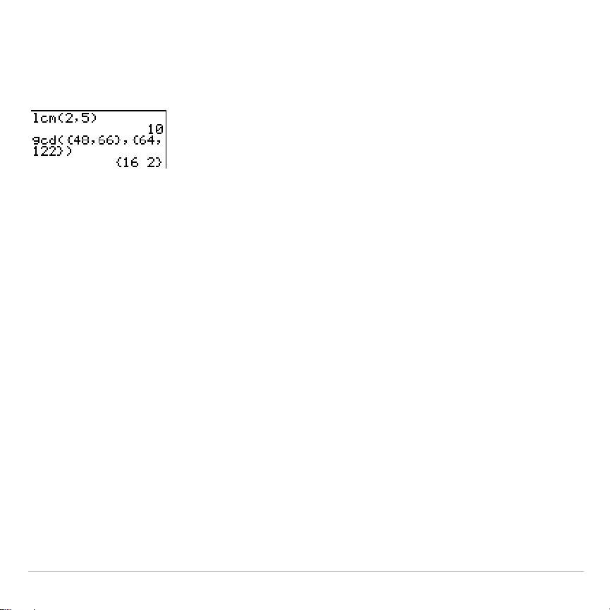
TI-83 Plus Math, Angle, and Test Operations 83
lcm(
valueA
,
valueB
) gcd(
valueA
,
valueB
)
lcm(
listA
,
listB
) gcd(
listA
,
listB
)
lcm(
list
,
value
) gcd(
list
,
value
)
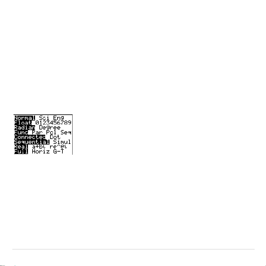
TI-83 Plus Math, Angle, and Test Operations 84
Entering and Using Complex Numbers
Complex-Number Modes
The TI-83 Plus displays complex numbers in rectangular form and polar
form. To select a complex-number mode, press
z
, and then select
either of the two modes.
•
a+b
i
(rectangular-complex mode)
•
re^
q
i
(polar-complex mode)
On the TI-83 Plus, complex numbers can be stored to variables. Also,
complex numbers are valid list elements.
In
Real
mode, complex-number results return an error, unless you
entered a complex number as input. For example, in
Real
mode
ln(
L
1)
returns an error; in
a+b
i
mode
ln(
L
1)
returns an answer.
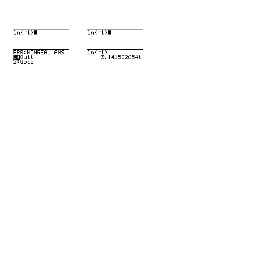
TI-83 Plus Math, Angle, and Test Operations 85
Real
mode
a+b
i
mode
$$
Entering Complex Numbers
Complex numbers are stored in rectangular form, but you can enter a
complex number in rectangular form or polar form, regardless of the
mode setting. The components of complex numbers can be real
numbers or expressions that evaluate to real numbers; expressions are
evaluated when the command is executed.
Note about Radian Versus Degree Mode
Radian mode is recommended for complex number calculations.
Internally, the TI-83 Plus converts all entered trigonometric values to
radians, but it does not convert values for exponential, logarithmic, or
hyperbolic functions.
In degree mode, complex identities such as
e
^(
i
q
) = cos(
q
) +
i
sin(
q
) are
not generally true because the values for cos and sin are converted to
radians, while those for e^() are not. For example,
e
^(
i
45) = cos(45)
+
i
sin(45) is treated internally as
e
^(
i
45) = cos(
p
/4) +
i
sin(
p
/4). Complex
identities are always true in radian mode.
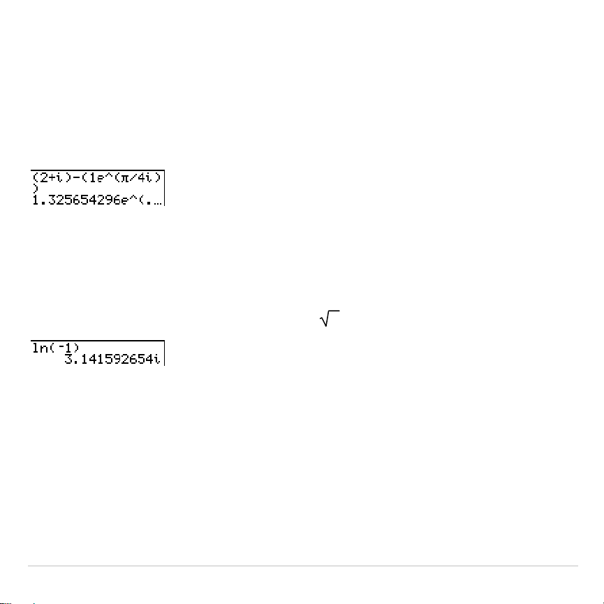
TI-83 Plus Math, Angle, and Test Operations 86
Interpreting Complex Results
Complex numbers in results, including list elements, are displayed in
either rectangular or polar form, as specified by the mode setting or by a
display conversion instruction. In the example below, polar-complex
(
re^
q
i)
and
Radian
modes are set.
Rectangular-Complex Mode
Rectangular-complex mode recognizes and displays a complex number in
the form
a+b
i
, where
a
is the real component,
b
is the imaginary
component, and
i
is a constant equal to
-1
.
To enter a complex number in rectangular form, enter the value of
a
(
real
component
), press
Ã
or
¹
, enter the value of
b
(
imaginary component
), and
press
y
V
(constant).
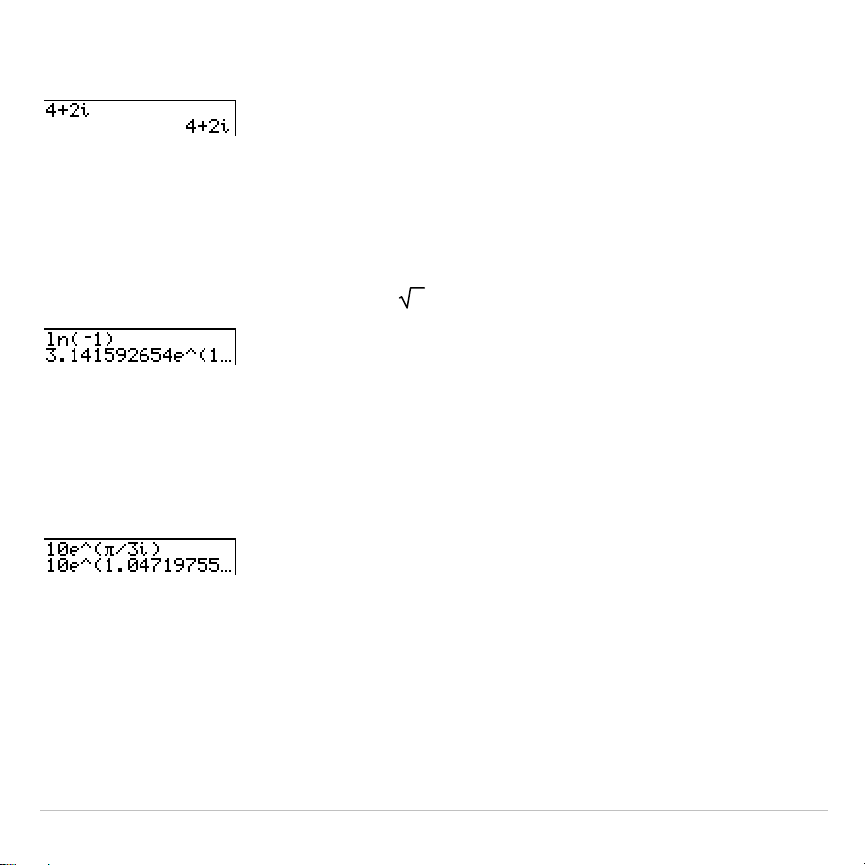
TI-83 Plus Math, Angle, and Test Operations 87
real component
(
+
or
N
)
imaginary component
i
Polar-Complex Mode
Polar-complex mode recognizes and displays a complex number in the
form
re^
q
i
, where
r
is the magnitude,
e
is the base of the natural log,
q
is the
angle, and
i
is a constant equal to
-1
.
To enter a complex number in polar form, enter the value of
r
(
magnitude
),
press
y
J
(exponential function), enter the value of
q
(
angle
), press
y
V
(constant), and then press
¤
.
magnitude
e^(
angle
i
)
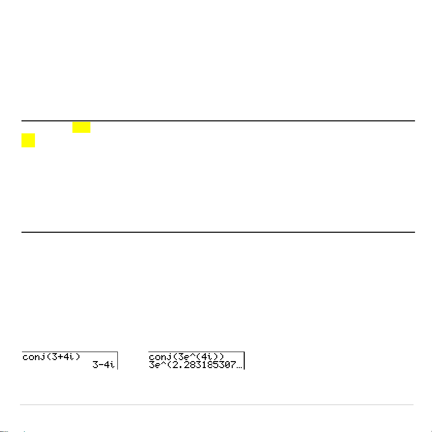
TI-83 Plus Math, Angle, and Test Operations 88
MATH CPX (Complex) Operations
MATH CPX Menu
To display the
MATH CPX
menu, press
~
~
.
MATH NUM CPX PRB
1: conj(
Returns the complex conjugate.
2: real(
Returns the real part.
3: imag(
Returns the imaginary part.
4: angle(
Returns the polar angle.
5: abs(
Returns the magnitude (modulus).
6:
4
Rect
Displays the result in rectangular form.
7:
4
Polar
Displays the result in polar form.
conj(
conj(
(conjugate) returns the complex conjugate of a complex number or
list of complex numbers.
conj(
a
+
b
i
)
returns
a
N
b
i
in
a+b
i
mode.
conj(
r
e^(
q
i
))
returns
r
e^(
Lq
i
)
in
re^
q
i
mode.
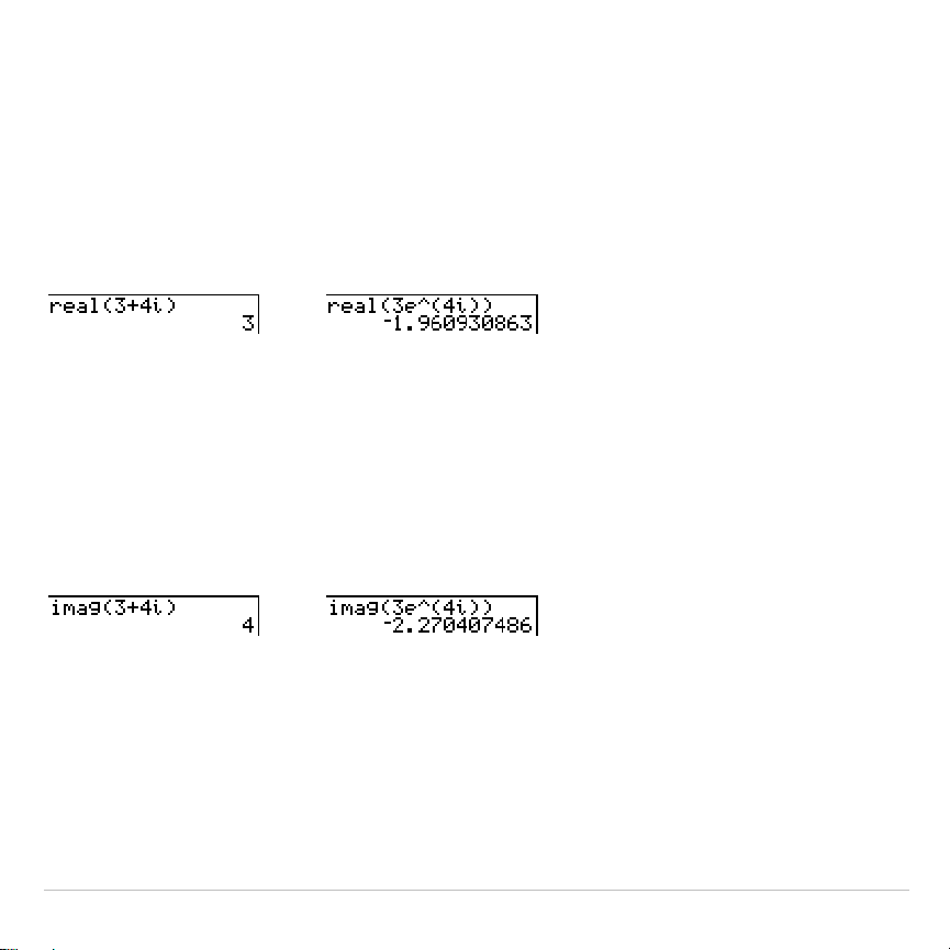
TI-83 Plus Math, Angle, and Test Operations 89
real(
real(
(real part) returns the real part of a complex number or list of
complex numbers.
real(
a
+
b
i
)
returns
a
.
real(
r
e^(
q
i
))
returns
r
ä
cos
(
q
).
imag(
imag(
(imaginary part) returns the imaginary (nonreal) part of a complex
number or list of complex numbers.
imag(
a
+
b
i
)
returns
b
.
imag(
r
e^(
q
i
))
returns
r
ä
sin(
q
)
.
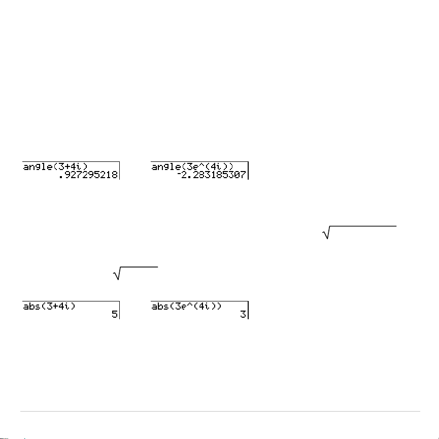
TI-83 Plus Math, Angle, and Test Operations 90
angle(
angle(
returns the polar angle of a complex number or list of complex
numbers, calculated as tan
L
1
(b/a), where b is the imaginary part and a is
the real part. The calculation is adjusted by +
p
in the second quadrant or
Np
in the third quadrant.
angle(
a
+
bi
)
returns
tan
L
1
(b/a)
.
angle(
r
e^(
q
i
))
returns
q
, where
Lp
<
q
<
p
.
abs(
abs(
(absolute value) returns the magnitude (modulus),
(real2+imag2)
, of
a complex number or list of complex numbers.
abs(
a
+
b
i
)
returns
(a2+b2)
.
abs(
r
e^(
q
i
))
returns
r
(magnitude).
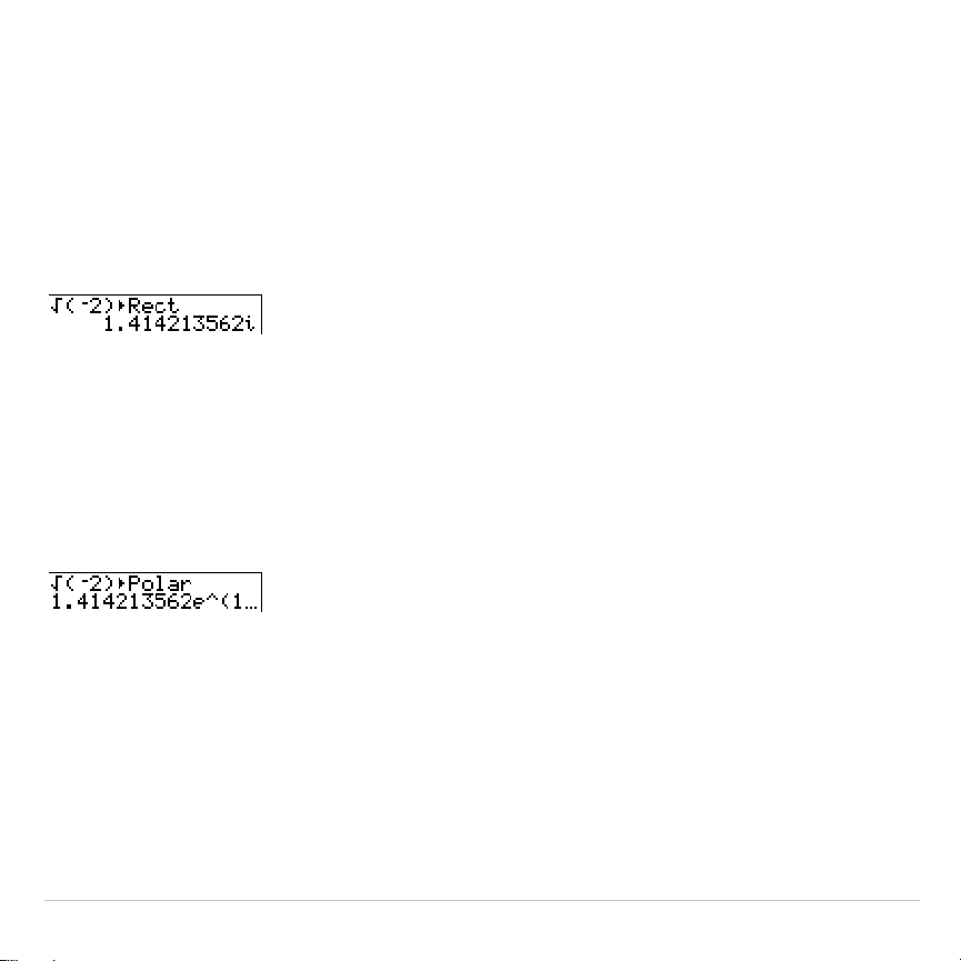
TI-83 Plus Math, Angle, and Test Operations 91
4
Rect
4
Rect
(display as rectangular) displays a complex result in rectangular
form. It is valid only at the end of an expression. It is not valid if the result
is real.
complex result
8
Rect
returns
a
+
b
i
.
4
Polar
4
Polar
(display as polar) displays a complex result in polar form. It is valid
only at the end of an expression. It is not valid if the result is real.
complex result
8
Polar
returns
r
e^(
q
i
)
.
TI-83 Plus Math, Angle, and Test Operations 92
MATH PRB (Probability) Operations
MATH PRB Menu
To display the
MATH PRB
menu, press
|
.
MATH NUM CPX PRB
1: rand
Random-number generator
2: nPr
Number of permutations
3: nCr
Number of combinations
4: !
Factorial
5: randInt(
Random-integer generator
6: randNorm(
Random # from Normal distribution
7: randBin(
Random # from Binomial distribution
rand
rand
(random number) generates and returns one or more random
numbers > 0 and < 1. To generate a list of random-numbers, specify an
integer > 1 for
numtrials
(number of trials). The default for
numtrials
is 1.
rand
[
(
numtrials
)
]
Tip: To generate random numbers beyond the range of 0 to 1, you can include
rand
in an expression. For example,
rand5
generates a random number > 0 and
< 5.

TI-83 Plus Math, Angle, and Test Operations 93
With each
rand
execution, the TI-83 Plus generates the same random-
number sequence for a given seed value. The TI-83 Plus factory-set
seed value for
rand
is
0
. To generate a different random-number
sequence, store any nonzero seed value to
rand
. To restore the factory-
set seed value, store
0
to
rand
or reset the defaults (Chapter 18).
Note: The seed value also affects
randInt(
,
randNorm(
, and
randBin(
instructions.
nPr, nCr
nPr
(number of permutations) returns the number of permutations of
items
taken
number
at a time.
items
and
number
must be nonnegative integers.
Both
items
and
number
can be lists.
items
nPr
number
nCr
(number of combinations) returns the number of combinations of
items
taken
number
at a time.
items
and
number
must be nonnegative
integers. Both
items
and
number
can be lists.
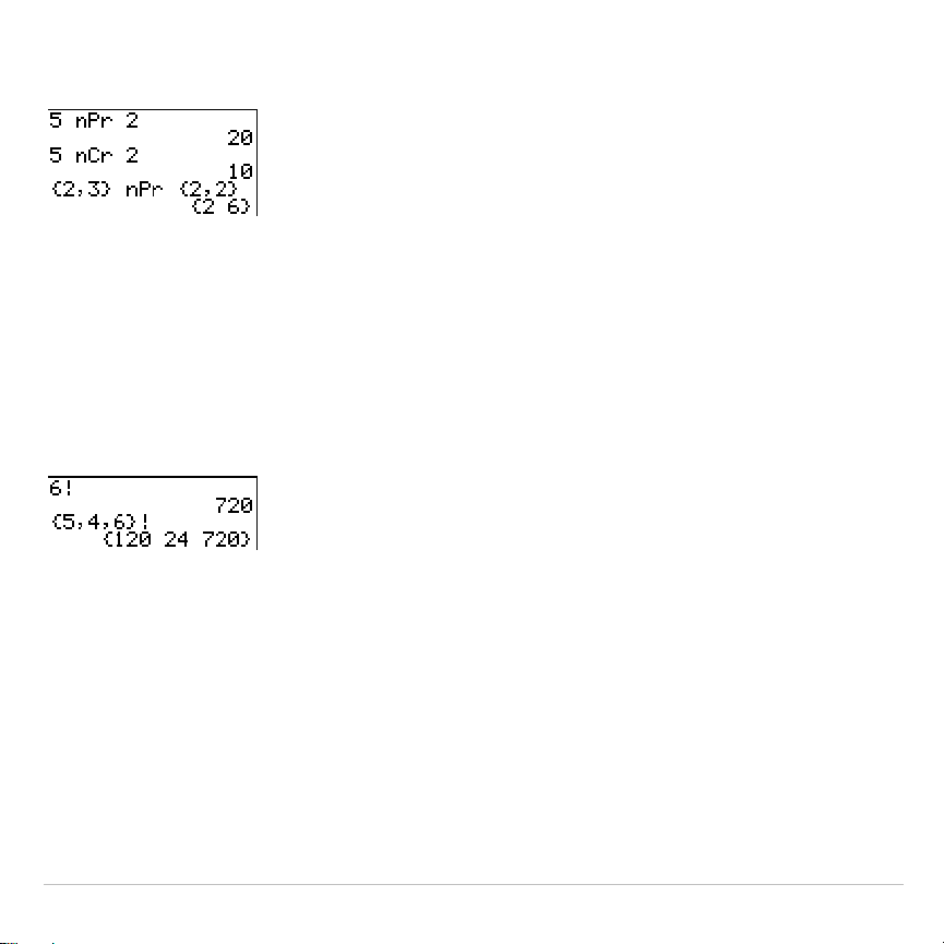
TI-83 Plus Math, Angle, and Test Operations 94
items
nCr
number
! (Factorial)
!
(factorial) returns the factorial of either an integer or a multiple of .5. For
a list, it returns factorials for each integer or multiple of .5.
value
must be
‚L
.5 and
69.
value
!
Note: The factorial is computed recursively using the relationship (n+1)! = n
ä
n!,
until n is reduced to either 0 or
L
1/2. At that point, the definition 0!=1 or the
definition (
L
1
à
2)!=
‡p
is used to complete the calculation. Hence:
n!=n
ä
(n
N
1)
ä
(n
N
2)
ä
...
ä
2
ä
1, if n is an integer
‚
0
n!= n
ä
(n
N
1)
ä
(n
N
2)
ä
...
ä
1
à
2
ä
‡p
, if n+1
à
2 is an integer
‚
0
n! is an error, if neither n nor n+1
à
2 is an integer
‚
0.
(The variable n equals
value
in the syntax description above.)
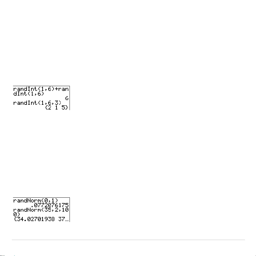
TI-83 Plus Math, Angle, and Test Operations 95
randInt(
randInt(
(random integer) generates and displays a random integer within
a range specified by
lower
and
upper
integer bounds. To generate a list of
random numbers, specify an integer >1 for
numtrials
(number of trials); if
not specified, the default is 1.
randInt(
lower
,
upper
[
,
numtrials
]
)
randNorm(
randNorm(
(random Normal) generates and displays a random real
number from a specified Normal distribution. Each generated value could
be any real number, but most will be within the interval [
mN
3(
s
),
m
+3(
s
)].
To generate a list of random numbers, specify an integer > 1 for
numtrials
(number of trials); if not specified, the default is 1.
randNorm(
m
,
s
[
,
numtrials
]
)
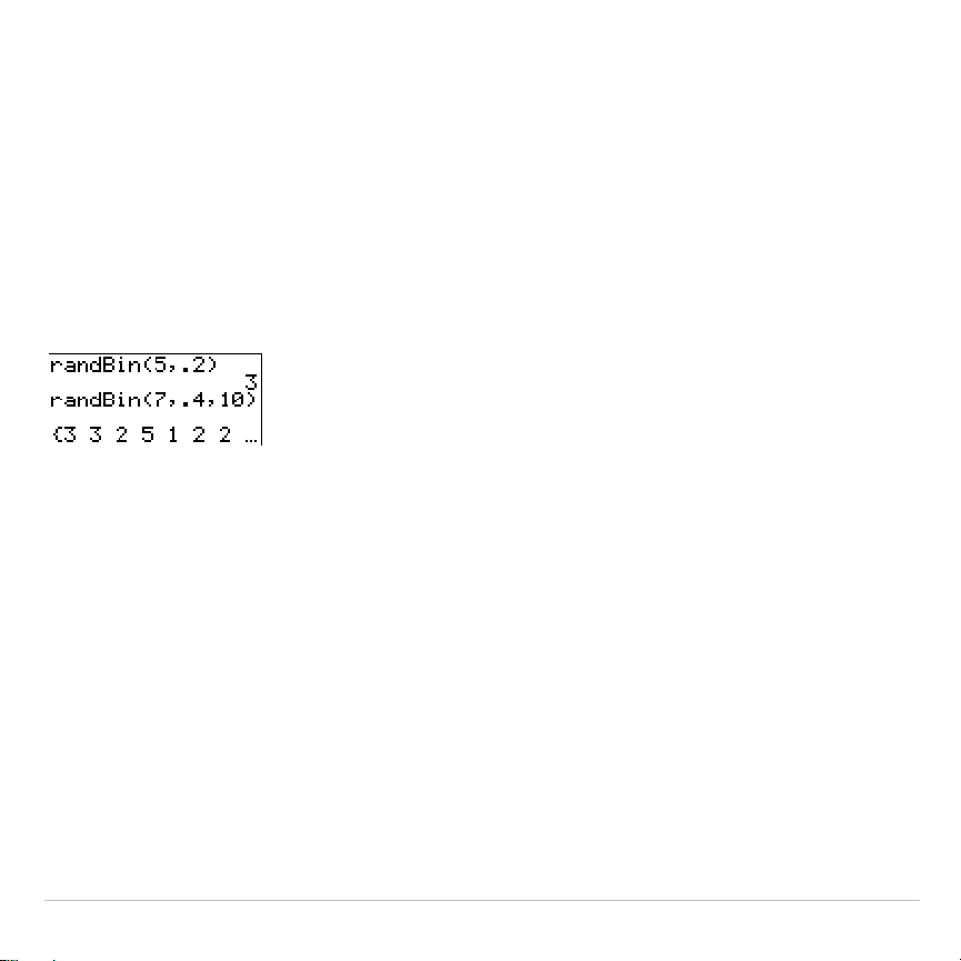
TI-83 Plus Math, Angle, and Test Operations 96
randBin(
randBin(
(random Binomial) generates and displays a random integer
from a specified Binomial distribution.
numtrials
(number of trials) must be
‚
1.
prob
(probability of success) must be
‚
0 and
1. To generate a list
of random numbers, specify an integer > 1 for
numsimulations
(number of
simulations); if not specified, the default is 1.
randBin(
numtrials
,
prob
[
,
numsimulations
]
)
Note: The seed value stored to
rand
also affects
randInt(
,
randNorm(
, and
randBin(
instructions.

TI-83 Plus Math, Angle, and Test Operations 97
ANGLE Operations
ANGLE Menu
To display the
ANGLE
menu, press
y
[
ANGLE
]. The
ANGLE
menu displays
angle indicators and instructions. The
Radian
/
Degree
mode setting affects
the TI-83 Plus’s interpretation of
ANGLE
menu entries.
ANGLE
1:
¡
Degree notation
2: '
DMS minute notation
3:
r
Radian notation
4:
8
DMS
Displays as degree/minute/second
5: R
8
Pr(
Returns
r
, given
X
and
Y
6: R
8
P
q
(
Returns
q
, given
X
and
Y
7: P
8
Rx(
Returns
x
, given
R
and
q
8: P
8
Ry(
Returns
y
, given
R
and
q
Entry Notation
DMS (degrees/minutes/seconds) entry notation comprises the degree
symbol (
¡
), the minute symbol (
'
), and the second symbol (
"
).
degrees
must be a real number;
minutes
and
seconds
must be real numbers
‚
0.
degrees
¡
minutes
'
seconds
"
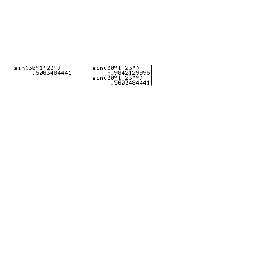
TI-83 Plus Math, Angle, and Test Operations 98
For example, enter for 30 degrees, 1 minute, 23 seconds. If the angle
mode is not set to
Degree
, you must use
¡
so that the TI-83 Plus can
interpret the argument as degrees, minutes, and seconds.
Degree
mode
Radian
mode
¡
(Degree)
¡
(degree) designates an angle or list of angles as degrees, regardless of
the current angle mode setting. In
Radian
mode, you can use
¡
to convert
degrees to radians.
value
¡
{
value1
,
value2
,
value3
,
value4
,
...
,
value n
}
¡
¡
also designates
degrees
(D) in DMS format.
'
(minutes) designates
minutes
(M) in DMS format.
"
(seconds) designates
seconds
(S) in DMS format.
Note:
"
is not on the
ANGLE
menu. To enter
"
, press
ƒ
[
ã
].
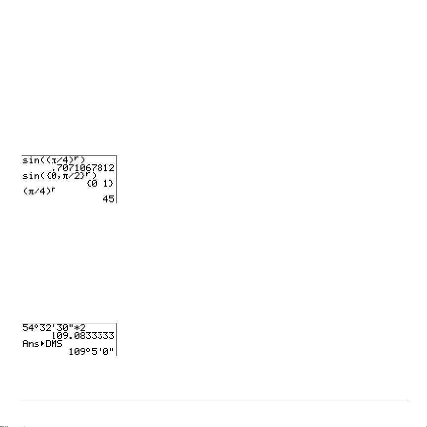
TI-83 Plus Math, Angle, and Test Operations 99
r
(Radians)
r
(radians) designates an angle or list of angles as radians, regardless of
the current angle mode setting. In
Degree
mode, you can use
r
to convert
radians to degrees.
value
r
Degree
mode
8
DMS
8
DMS
(degree/minute/second) displays
answer
in DMS format. The mode
setting must be
Degree
for
answer
to be interpreted as degrees, minutes,
and seconds.
8
DMS
is valid only at the end of a line.
answer
8
DMS
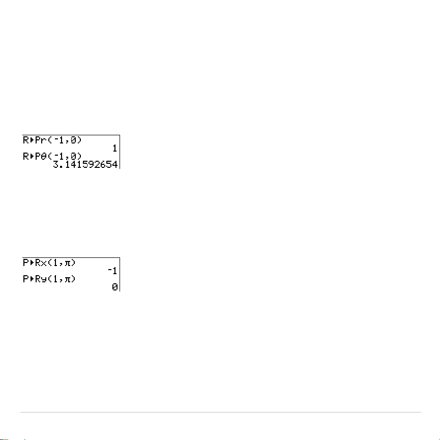
TI-83 Plus Math, Angle, and Test Operations 100
R
8
Pr(, R
8
P
q
(, P
8
Rx(, P
8
Ry(
R
8
Pr(
converts rectangular coordinates to polar coordinates and returns
r
.
R
8
P
q
(
converts rectangular coordinates to polar coordinates and
returns
q
.
x
and
y
can be lists.
R
8
Pr(
x
,
y
), R
8
P
q
(
x
,
y
)
Note:
Radian
mode is set.
P
8
Rx(
converts polar coordinates to rectangular coordinates and returns
x
.
P
8
Ry(
converts polar coordinates to rectangular coordinates and
returns
y
.
r
and
q
can be lists.
P
8
Rx(
r
,
q
), P
8
Ry(
r
,
q
)
Note:
Radian
mode is set.
TI-83 Plus Math, Angle, and Test Operations 101
TEST (Relational) Operations
TEST Menu
To display the
TEST
menu, press
y
:
.
This operator... Returns 1 (true) if...
TEST LOGIC
1:
=
Equal
2:
ƒ
Not equal to
3:
>
Greater than
4:
‚
Greater than or equal to
5:
<
Less than
6:
Less than or equal to
=,
ƒ
, >,
‚
, <,
Relational operators compare
valueA
and
valueB
and return
1
if the test is
true or
0
if the test is false.
valueA
and
valueB
can be real numbers,
expressions, or lists. For
=
and
ƒ
only,
valueA
and
valueB
also can be
matrices or complex numbers. If
valueA
and
valueB
are matrices, both
must have the same dimensions.
Relational operators are often used in programs to control program flow
and in graphing to control the graph of a function over specific values.
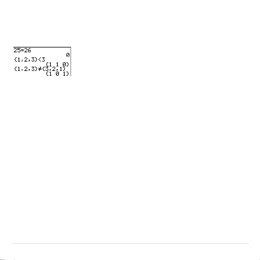
TI-83 Plus Math, Angle, and Test Operations 102
valueA
=
valueB valueA
ƒ
valueB
valueA
>
valueB valueA
‚
valueB
valueA
<
valueB valueA
valueB
Using Tests
Relational operators are evaluated after mathematical functions
according to EOS rules (Chapter 1).
•
The expression
2+2=2+3
returns
0
. The TI-83 Plus performs the
addition first because of EOS rules, and then it compares 4 to 5.
•
The expression
2+(2=2)+3
returns
6
. The TI-83 Plus performs the
relational test first because it is in parentheses, and then it adds 2, 1,
and 3.
TI-83 Plus Math, Angle, and Test Operations 103
TEST LOGIC (Boolean) Operations
TEST LOGIC Menu
To display the
TEST LOGIC
menu, press
y
ã
TESTä
~
.
This operator... Returns a 1 (true) if...
TEST LOGIC
1: and
Both values are nonzero (true).
2: or
At least one value is nonzero (true).
3: xor
Only one value is zero (false).
4: not(
The value is zero (false).
Boolean Operators
Boolean operators are often used in programs to control program flow
and in graphing to control the graph of the function over specific values.
Values are interpreted as zero (false) or nonzero (true).
and, or, xor
and
,
or
, and
xor
(exclusive or) return a value of
1
if an expression is true
or
0
if an expression is false, according to the table below.
valueA
and
valueB
can be real numbers, expressions, or lists.
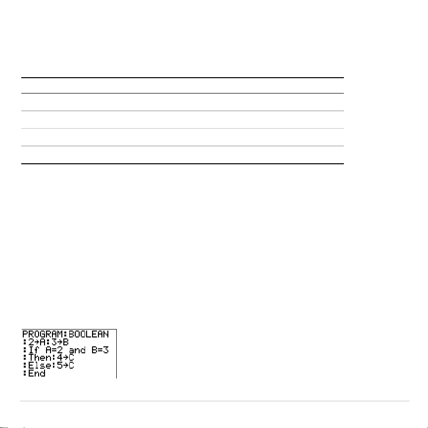
TI-83 Plus Math, Angle, and Test Operations 104
valueA
and
valueB
valueA
or
valueB
valueA
xor
valueB
valueA valueB and or xor
ƒ
0
ƒ
0 returns 1 1 0
ƒ
0 0 returns 0 1 1
0
ƒ
0 returns 0 1 1
0 0 returns 0 0 0
not(
not(
returns
1
if
value
(which can be an expression) is
0
.
not(
value
)
Using Boolean Operations
Boolean logic is often used with relational tests. In the following program,
the instructions store
4
into
C
.
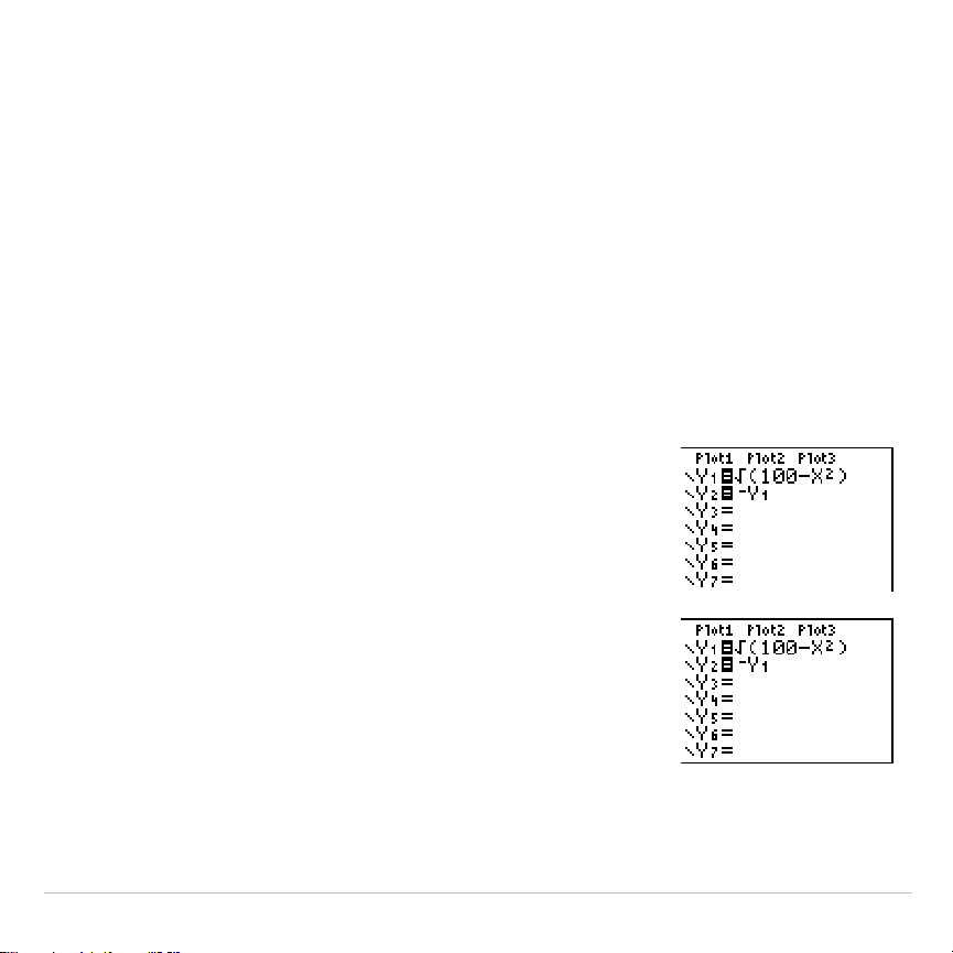
TI-83 Plus Function Graphing 105
Chapter 3:
Function Graphing
Getting Started: Graphing a Circle
Getting Started is a fast-paced introduction. Read the chapter for details.
Graph a circle of radius 10, centered on the origin in the standard viewing
window. To graph this circle, you must enter separate formulas for the upper and
lower portions of the circle. Then use ZSquare (zoom square) to adjust the
display and make the functions appear as a circle.
1. In
Func
mode, press
o
to display the
Y=
editor.
Press
y
ã
‡
ä
100
¹
„
¡
¤
Í
to
enter the expression Y=
‡
(100
N
X
2
), which
defines the top half of the circle.
The expression Y=
L‡
(100
N
X
2
) defines the
bottom half of the circle. On the TI-83 Plus, you
can define one function in terms of another. To
define
Y
2
=
L
Y
1
, press
Ì
to enter the negation
sign. Press
~
to display the
VARS Y
.
VARS
menu. Then press
Í
to select
1:Function
.
The
FUNCTION
secondary menu is displayed.
Press
1
to select
1:Y
1
.
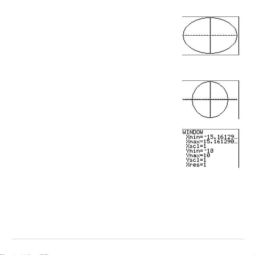
TI-83 Plus Function Graphing 106
2. Press
q
6
to select
6:ZStandard
. This is a
quick way to reset the window variables to the
standard values. It also graphs the functions;
you do not need to press
s
.
Notice that the functions appear as an ellipse in
the standard viewing window.
3. To adjust the display so that each pixel
represents an equal width and height, press
q
5
to select
5:ZSquare
. The functions are
replotted and now appear as a circle on the
display.
4. To see the
ZSquare
window variables, press
p
and notice the new values for
Xmin
,
Xmax
,
Ymin
, and
Ymax
.

TI-83 Plus Function Graphing 107
Defining Graphs
TI-83 Plus—Graphing Mode Similarities
Chapter 3 specifically describes function graphing, but the steps shown
here are similar for each TI-83 Plus graphing mode. Chapters 4, 5, and 6
describe aspects that are unique to parametric graphing, polar graphing,
and sequence graphing.
Defining a Graph
To define a graph in any graphing mode, follow these steps. Some steps
are not always necessary.
1. Press
z
and set the appropriate graph mode.
2. Press
o
and enter, edit, or select one or more functions in the
Y=
editor.
3. Deselect stat plots, if necessary.
4. Set the graph style for each function.
5. Press
p
and define the viewing window variables.
6. Press
y
.
and select the graph format settings.

TI-83 Plus Function Graphing 108
Displaying and Exploring a Graph
After you have defined a graph, press
s
to display it. Explore the
behavior of the function or functions using the TI-83 Plus tools described
in this chapter.
Saving a Graph for Later Use
You can store the elements that define the current graph to any of 10
graph database variables (
GDB1
through
GDB9
, and
GDB0
; Chapter 8).
To recreate the current graph later, simply recall the graph database to
which you stored the original graph.
These types of information are stored in a
GDB
.
•
Y=
functions
•
Graph style settings
•
Window settings
•
Format settings
You can store a picture of the current graph display to any of 10 graph
picture variables (
Pic1
through
Pic9
, and
Pic0
; Chapter 8). Then you can
superimpose one or more stored pictures onto the current graph.
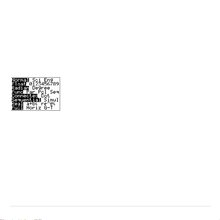
TI-83 Plus Function Graphing 109
Setting the Graph Modes
Checking and Changing the Graphing Mode
To display the mode screen, press
z
. The default settings are
highlighted below. To graph functions, you must select
Func
mode
before you enter values for the window variables and before you enter
the functions.
The TI-83 Plus has four graphing modes.
•
Func
(function graphing)
•
Par
(parametric graphing; Chapter 4)
•
Pol
(polar graphing; Chapter 5)
•
Seq
(sequence graphing; Chapter 6)
Other mode settings affect graphing results. Chapter 1 describes each
mode setting.

TI-83 Plus Function Graphing 110
•
Float
or
0123456789
(fixed) decimal mode affects displayed graph
coordinates.
•
Radian
or
Degree
angle mode affects interpretation of some functions.
•
Connected
or
Dot
plotting mode affects plotting of selected functions.
•
Sequential
or
Simul
graphing-order mode affects function plotting
when more than one function is selected.
Setting Modes from a Program
To set the graphing mode and other modes from a program, begin on a
blank line in the program editor and follow these steps.
1. Press
z
to display the mode settings.
2. Press
†
,
~
,
|
, and
}
to place the cursor on the mode that you
want to select.
3. Press
Í
to paste the mode name to the cursor location.
The mode is changed when the program is executed.
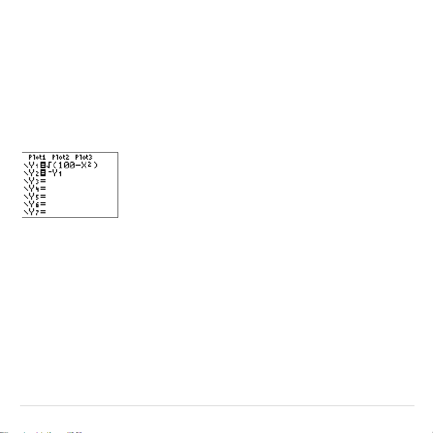
TI-83 Plus Function Graphing 111
Defining Functions
Displaying Functions in the Y= Editor
To display the
Y=
editor, press
o
. You can store up to 10 functions to
the function variables
Y1
through
Y9
, and
Y0
. You can graph one or more
defined functions at once. In this example, functions
Y1
and
Y2
are
defined and selected.
Defining or Editing a Function
To define or edit a function, follow these steps.
1. Press
o
to display the
Y=
editor.
2. Press
†
to move the cursor to the function you want to define or edit.
To erase a function, press
‘
.
3. Enter or edit the expression to define the function.

TI-83 Plus Function Graphing 112
•
You may use functions and variables (including matrices and lists)
in the expression. When the expression evaluates to a nonreal
number, the value is not plotted; no error is returned.
•
The independent variable in the function is
X
.
Func
mode defines
„
as
X
. To enter
X
, press
„
or press
ƒ
[
X
].
•
When you enter the first character, the
=
is highlighted, indicating
that the function is selected.
As you enter the expression, it is stored to the variable
Y
n
as a user-
defined function in the
Y=
editor.
4. Press
Í
or
†
to move the cursor to the next function.
Defining a Function from the Home Screen or a Program
To define a function from the home screen or a program, begin on a
blank line and follow these steps.
1. Press
ƒ
[
ã
], enter the expression, and then press
ƒ
[
ã
]
again.
2. Press
¿
.
3. Press
~
1
to select
1:Function
from the
VARS Y
.
VARS
menu.
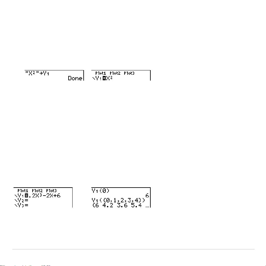
TI-83 Plus Function Graphing 113
4. Select the function name, which pastes the name to the cursor
location on the home screen or program editor.
5. Press
Í
to complete the instruction.
"
expression
"
!
Y
n
When the instruction is executed, the TI-83 Plus stores the expression to
the designated variable
Y
n
, selects the function, and displays the
message
Done
.
Evaluating Y= Functions in Expressions
You can calculate the value of a
Y=
function
Y
n
at a specified
value
of
X
. A
list of
values
returns a list.
Y
n
(
value
)
Y
n
({
value1,value2,value3, . . .,value n
})

TI-83 Plus Function Graphing 114
Selecting and Deselecting Functions
Selecting and Deselecting a Function
You can select and deselect (turn on and turn off) a function in the
Y=
editor. A function is selected when the
=
sign is highlighted. The
TI-83 Plus graphs only the selected functions. You can select any or all
functions
Y1
through
Y9
, and
Y0
.
To select or deselect a function in the
Y=
editor, follow these steps.
1. Press
o
to display the
Y=
editor.
2. Move the cursor to the function you want to select or deselect.
3. Press
|
to place the cursor on the function’s
=
sign.
4. Press
Í
to change the selection status.
When you enter or edit a function, it is selected automatically. When you
clear a function, it is deselected.

TI-83 Plus Function Graphing 115
Turning On or Turning Off a Stat Plot in the Y= Editor
To view and change the on/off status of a stat plot in the
Y=
editor, use
Plot1 Plot2 Plot3
(the top line of the
Y=
editor). When a plot is on, its name
is highlighted on this line.
To change the on/off status of a stat plot from the
Y=
editor, press
}
and
~
to place the cursor on
Plot1
,
Plot2
, or
Plot3
, and then press
Í
.
Selecting and Deselecting Functions from the Home Screen or a
Program
To select or deselect a function from the home screen or a program,
begin on a blank line and follow these steps.
1. Press
~
to display the
VARS Y
.
VARS
menu.
2. Select
4:On/Off
to display the
ON/OFF
secondary menu.
Plot1
is turned on.
Plot2
and
Plot3
are turned off.
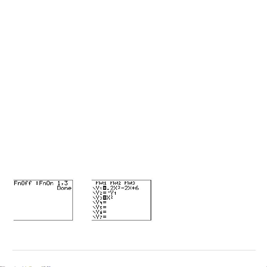
TI-83 Plus Function Graphing 116
3. Select
1:FnOn
to turn on one or more functions or
2:FnOff
to turn off
one or more functions. The instruction you select is copied to the
cursor location.
4. Enter the number (
1
through
9
, or
0
; not the variable
Y
n
) of each
function you want to turn on or turn off.
•
If you enter two or more numbers, separate them with commas.
•
To turn on or turn off all functions, do not enter a number after
FnOn
or
FnOff
.
FnOn
[
function#,function#, . . .,function n
]
FnOff
[
function#,function#, . . .,function n
]
5. Press
Í
. When the instruction is executed, the status of each
function in the current mode is set and
Done
is displayed.
For example, in
Func
mode,
FnOff :FnOn 1,3
turns off all functions in the
Y=
editor, and then turns on
Y1
and
Y3
.

TI-83 Plus Function Graphing 117
Setting Graph Styles for Functions
Graph Style Icons in the Y= Editor
This table describes the graph styles available for function graphing. Use
the styles to visually differentiate functions to be graphed together. For
example, you can set
Y1
as a solid line,
Y2
as a dotted line, and
Y3
as a
thick line.
Icon Style Description
ç
Line A solid line connects plotted points; this is the default in
Connected
mode
è
Thick A thick solid line connects plotted points
é
Above Shading covers the area above the graph
ê
Below Shading covers the area below the graph
ë
Path A circular cursor traces the leading edge of the graph and
draws a path
ì
Animate A circular cursor traces the leading edge of the graph
without drawing a path
í
Dot A small dot represents each plotted point; this is the
default in
Dot
mode
Note: Some graph styles are not available in all graphing modes. Chapters 4,
5, and 6 list the styles for
Par
,
Pol
, and
Seq
modes.
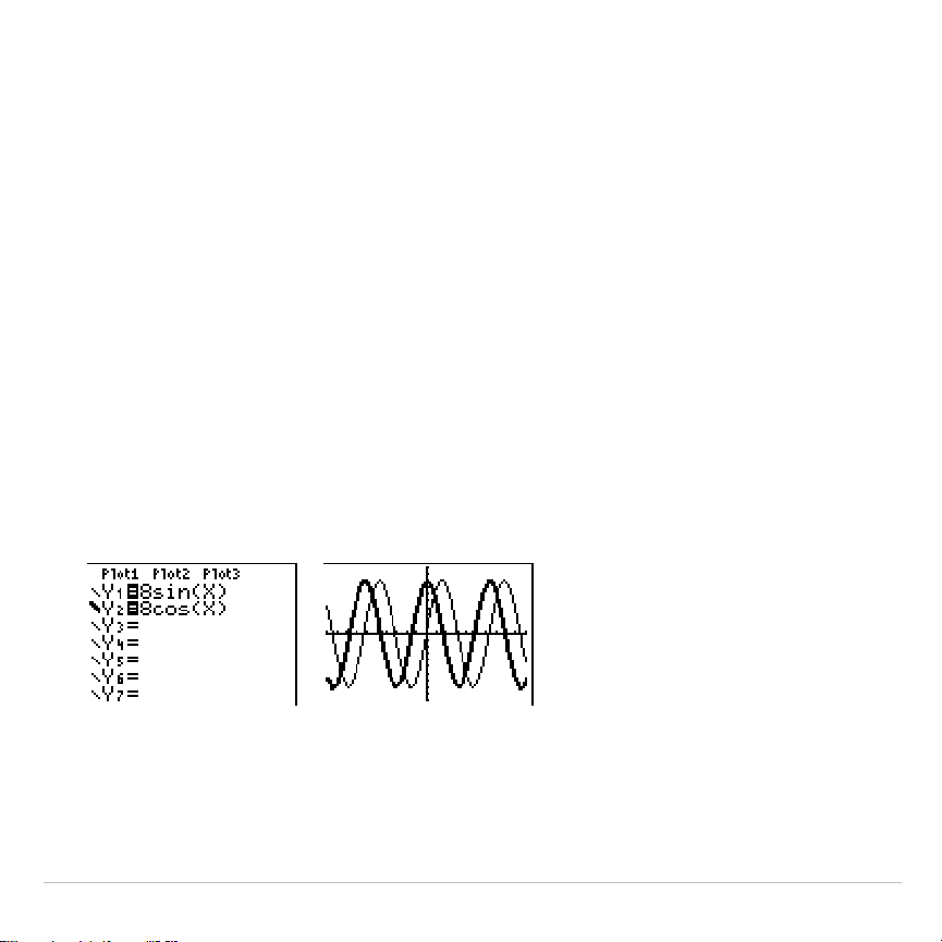
TI-83 Plus Function Graphing 118
Setting the Graph Style
To set the graph style for a function, follow these steps.
1. Press
o
to display the
Y=
editor.
2. Press
†
and
}
to move the cursor to the function.
3. Press
|
|
to move the cursor left, past the
=
sign, to the graph style
icon in the first column. The insert cursor is displayed. (Steps 2 and 3
are interchangeable.)
4. Press
Í
repeatedly to rotate through the graph styles. The seven
styles rotate in the same order in which they are listed in the table
above.
5. Press
~
,
}
, or
†
when you have selected a style.
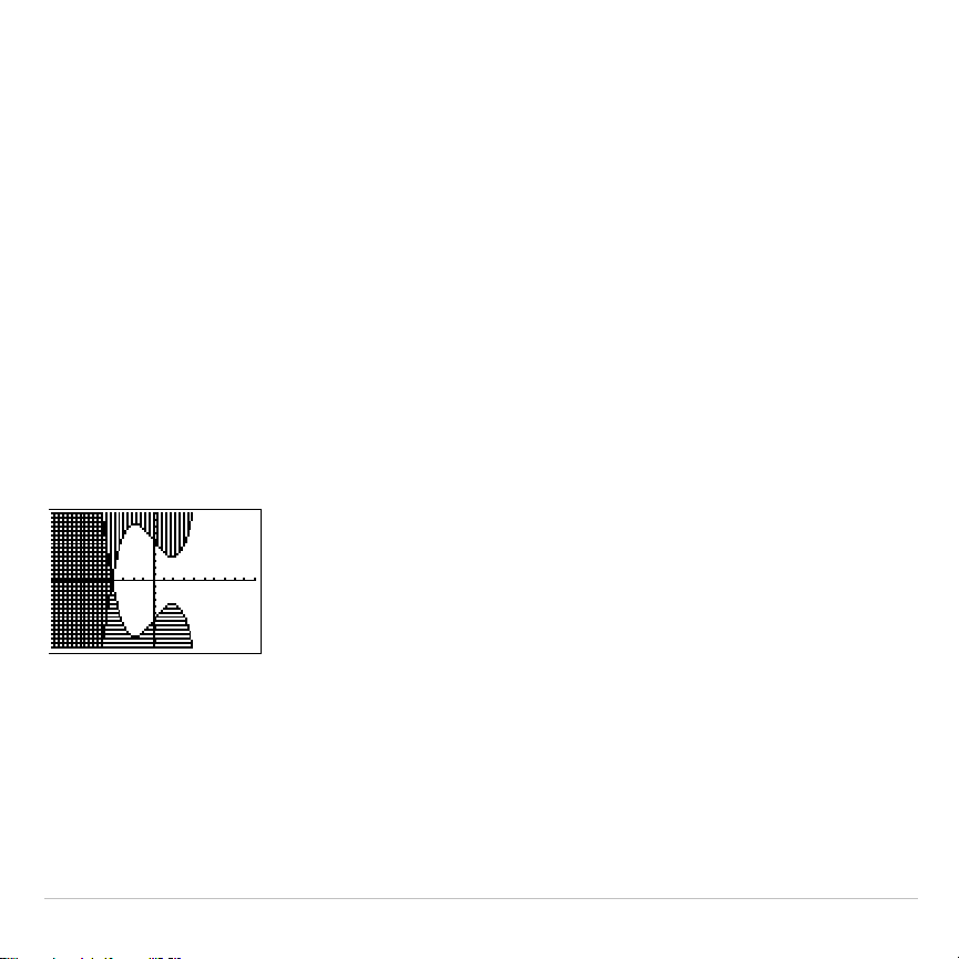
TI-83 Plus Function Graphing 119
Shading Above and Below
When you select
é
or
ê
for two or more functions, the TI-83 Plus rotates
through four shading patterns.
•
Vertical lines shade the first function with a
é
or
ê
graph style.
•
Horizontal lines shade the second.
•
Negatively sloping diagonal lines shade the third.
•
Positively sloping diagonal lines shade the fourth.
•
The rotation returns to vertical lines for the fifth
é
or
ê
function,
repeating the order described above.
When shaded areas intersect, the patterns overlap.
Note: When
é
or
ê
is selected for a Y= function that graphs a family of curves,
such as
Y1={1,2,3}X
, the four shading patterns rotate for each member of the
family of curves.
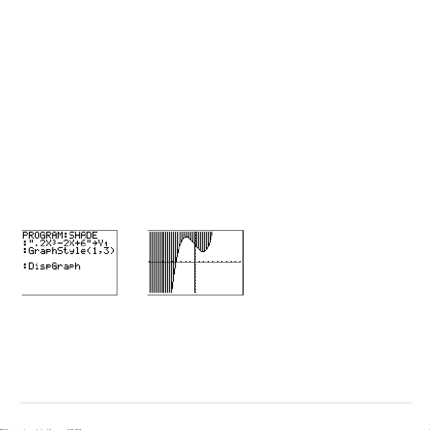
TI-83 Plus Function Graphing 120
Setting a Graph Style from a Program
To set the graph style from a program, select
H:GraphStyle(
from the
PRGM CTL
menu. To display this menu, press
while in the program
editor.
function#
is the number of the
Y=
function name in the current
graphing mode.
graphstyle#
is an integer from
1
to
7
that corresponds to
the graph style, as shown below.
1
=
ç
(line)
2
=
è
(thick)
3
=
é
(above)
4
=
ê
(below)
5
=
ë
(path)
6
=
ì
(animate)
7
=
í
(dot)
GraphStyle(
function#,graphstyle#
)
For example, when this program is executed in
Func
mode,
GraphStyle(1,3)
sets
Y1
to
é
(above).
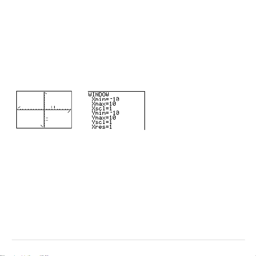
TI-83 Plus Function Graphing 121
Setting the Viewing Window Variables
The TI-83 Plus Viewing Window
The viewing window is the portion of the coordinate plane defined by
Xmin
,
Xmax
,
Ymin
, and
Ymax
.
Xscl
(X scale) defines the distance between
tick marks on the x-axis.
Yscl
(Y scale) defines the distance between tick
marks on the y-axis. To turn off tick marks, set
Xscl=0
and
Yscl=0
.
Xmax
Ymin
Ymax
Xscl
Yscl
Xmin
Displaying the Window Variables
To display the current window variable values, press
p
. The
window editor above and to the right shows the default values in
Func
graphing mode and
Radian
angle mode. The window variables differ from
one graphing mode to another.
Xres
sets pixel resolution (
1
through
8
) for function graphs only. The
default is
1
.
•
At
Xres=1
, functions are evaluated and graphed at each pixel on the
x-axis.

TI-83 Plus Function Graphing 122
•
At
Xres=8
, functions are evaluated and graphed at every eighth pixel
along the x-axis.
Tip: Small Xres values improve graph resolution but may cause the TI-83 Plus
to draw graphs more slowly.
Changing a Window Variable Value
To change a window variable value from the window editor, follow these
steps.
1. Press
†
or
}
to move the cursor to the window variable you want to
change.
2. Edit the value, which can be an expression.
•
Enter a new value, which clears the original value.
•
Move the cursor to a specific digit, and then edit it.
3. Press
Í
,
†
, or
}
. If you entered an expression, the TI-83 Plus
evaluates it. The new value is stored.
Note:
Xmin
<
Xmax
and
Ymin
<
Ymax
must be true in order to graph.

TI-83 Plus Function Graphing 123
Storing to a Window Variable from the Home Screen or a Program
To store a value, which can be an expression, to a window variable,
begin on a blank line and follow these steps.
1. Enter the value you want to store.
2. Press
¿
.
3. Press
to display the
VARS
menu.
4. Select
1:Window
to display the
Func
window variables (
X/Y
secondary
menu).
•
Press
~
to display the
Par
and
Pol
window variables (
T/
q
secondary menu).
•
Press
~
~
to display the
Seq
window variables (
U/V/W
secondary
menu).
5. Select the window variable to which you want to store a value. The
name of the variable is pasted to the current cursor location.
6. Press
Í
to complete the instruction.
TI-83 Plus Function Graphing 124
When the instruction is executed, the TI-83 Plus stores the value to the
window variable and displays the value.
@
X and
@
Y
The variables
@
X
and
@
Y
(items
8
and
9
on the
VARS
(
1:Window
)
X/Y
secondary menu) define the distance from the center of one pixel to the
center of any adjacent pixel on a graph (graphing accuracy).
@
X
and
@
Y
are calculated from
Xmin
,
Xmax
,
Ymin
, and
Ymax
when you display a
graph.
@
X
=
(Xmax
N
Xmin)
94
@
Y
=
(Ymax
N
Ymin)
62
You can store values to
@
X
and
@
Y
. If you do,
Xmax
and
Ymax
are
calculated from
@
X
,
Xmin
,
@
Y
, and
Ymin
.
TI-83 Plus Function Graphing 125
Setting the Graph Format
Displaying the Format Settings
To display the format settings, press
y
.
. The default settings
are highlighted below.
RectGC PolarGC
Sets cursor coordinates.
CoordOn CoordOff
Sets coordinates display on or off.
GridOff GridOn
Sets grid off or on.
AxesOn AxesOff
Sets axes on or off.
LabelOff LabelOn
Sets axes label off or on.
ExprOn ExprOff
Sets expression display on or off.
Format settings define a graph’s appearance on the display. Format
settings apply to all graphing modes.
Seq
graphing mode has an
additional mode setting (Chapter 6).
Changing a Format Setting
To change a format setting, follow these steps.
1. Press
†
,
~
,
}
, and
|
as necessary to move the cursor to the
setting you want to select.
2. Press
Í
to select the highlighted setting.

TI-83 Plus Function Graphing 126
RectGC, PolarGC
RectGC
(rectangular graphing coordinates) displays the cursor location
as rectangular coordinates
X
and
Y
.
PolarGC
(polar graphing coordinates) displays the cursor location as
polar coordinates
R
and
q
.
The
RectGC
/
PolarGC
setting determines which variables are updated
when you plot the graph, move the free-moving cursor, or trace.
•
RectGC
updates
X
and
Y
; if
CoordOn
format is selected,
X
and
Y
are
displayed.
•
PolarGC
updates
X
,
Y
,
R
, and
q
; if
CoordOn
format is selected,
R
and
q
are displayed.
CoordOn, CoordOff
CoordOn
(coordinates on) displays the cursor coordinates at the bottom
of the graph. If
ExprOff
format is selected, the function number is
displayed in the top-right corner.
CoordOff
(coordinates off) does not display the function number or
coordinates.

TI-83 Plus Function Graphing 127
GridOff, GridOn
Grid points cover the viewing window in rows that correspond to the tick
marks on each axis.
GridOff
does not display grid points.
GridOn
displays grid points.
AxesOn, AxesOff
AxesOn
displays the axes.
AxesOff
does not display the axes.
This overrides the
LabelOff
/
LabelOn
format setting.
LabelOff, LabelOn
LabelOff
and
LabelOn
determine whether to display labels for the axes (
X
and
Y
), if
AxesOn
format is also selected.

TI-83 Plus Function Graphing 128
ExprOn, ExprOff
ExprOn
and
ExprOff
determine whether to display the
Y=
expression
when the trace cursor is active. This format setting also applies to stat
plots.
When
ExprOn
is selected, the expression is displayed in the top-left
corner of the graph screen.
When
ExprOff
and
CoordOn
both are selected, the number in the top-right
corner specifies which function is being traced.

TI-83 Plus Function Graphing 129
Displaying Graphs
Displaying a New Graph
To display the graph of the selected function or functions, press
s
.
TRACE
,
ZOOM
instructions, and
CALC
operations display the graph
automatically. As the TI-83 Plus plots the graph, the busy indicator is on.
As the graph is plotted,
X
and
Y
are updated.
Pausing or Stopping a Graph
While plotting a graph, you can pause or stop graphing.
•
Press
Í
to pause; then press
Í
to resume.
•
Press
É
to stop; then press
s
to redraw.
Smart Graph
Smart Graph is a TI-83 Plus feature that redisplays the last graph
immediately when you press
s
, but only if all graphing factors that
would cause replotting have remained the same since the graph was last
displayed.
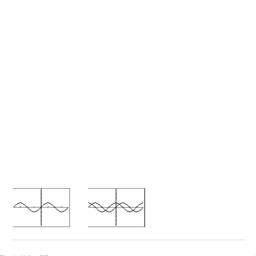
TI-83 Plus Function Graphing 130
If you performed any of these actions since the graph was last displayed,
the TI-83 Plus will replot the graph based on new values when you press
s
.
•
Changed a mode setting that affects graphs
•
Changed a function in the current picture
•
Selected or deselected a function or stat plot
•
Changed the value of a variable in a selected function
•
Changed a window variable or graph format setting
•
Cleared drawings by selecting
ClrDraw
•
Changed a stat plot definition
Overlaying Functions on a Graph
On the TI-83 Plus, you can graph one or more new functions without
replotting existing functions. For example, store
sin(X)
to
Y1
in the
Y=
editor and press
s
. Then store
cos(X)
to
Y2
and press
s
again. The function
Y2
is graphed on top of
Y1
, the original function.
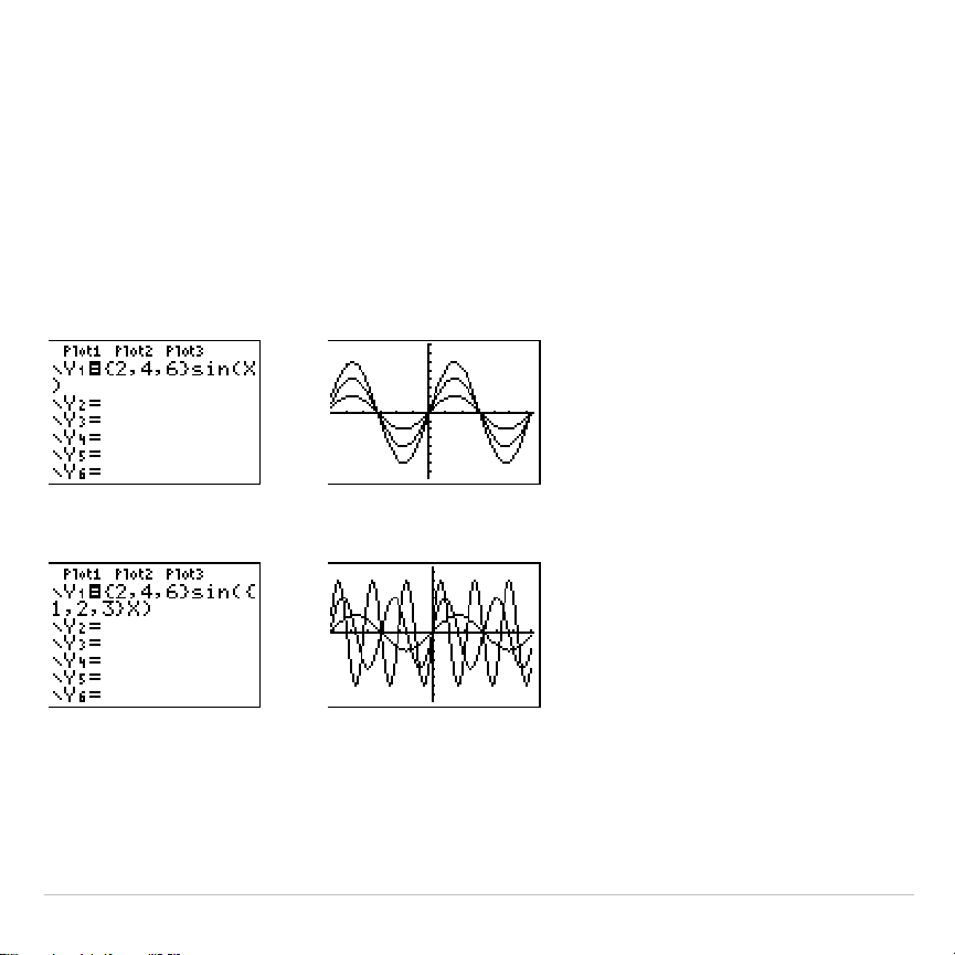
TI-83 Plus Function Graphing 131
Graphing a Family of Curves
If you enter a list (Chapter 11) as an element in an expression, the
TI-83 Plus plots the function for each value in the list, thereby graphing a
family of curves. In
Simul
graphing-order mode, it graphs all functions
sequentially for the first element in each list, and then for the second,
and so on.
{2,4,6}sin(X)
graphs three functions:
2 sin(X)
,
4 sin(X)
, and
6 sin(X)
.
{2,4,6}sin({1,2,3}X)
graphs
2 sin(X)
,
4 sin(2X)
, and
6 sin(3X)
.
Note: When using more than one list, the lists must have the same dimensions.

TI-83 Plus Function Graphing 132
Exploring Graphs with the Free-Moving
Cursor
Free-Moving Cursor
When a graph is displayed, press
|
,
~
,
}
, or
†
to move the cursor
around the graph. When you first display the graph, no cursor is visible.
When you press
|
,
~
,
}
, or
†
, the cursor moves from the center of the
viewing window.
As you move the cursor around the graph, the coordinate values of the
cursor location are displayed at the bottom of the screen if
CoordOn
format is selected. The
Float
/
Fix
decimal mode setting determines the
number of decimal digits displayed for the coordinate values.
To display the graph with no cursor and no coordinate values, press
‘
or
Í
. When you press
|
,
~
,
}
, or
†
, the cursor moves from
the same position.
Graphing Accuracy
The free-moving cursor moves from pixel to pixel on the screen. When
you move the cursor to a pixel that appears to be on the function, the
cursor may be near, but not actually on, the function. The coordinate
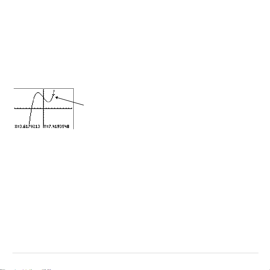
TI-83 Plus Function Graphing 133
value displayed at the bottom of the screen actually may not be a point
on the function. To move the cursor along a function, use
r
.
The coordinate values displayed as you move the cursor approximate
actual math coordinates, *accurate to within the width and height of the
pixel. As
Xmin
,
Xmax
,
Ymin
, and
Ymax
get closer together (as in a
Zoom
In
) graphing accuracy increases, and the coordinate values more closely
approximate the math coordinates.
Free- moving cursor “on” the
curve

TI-83 Plus Function Graphing 134
Exploring Graphs with TRACE
Beginning a Trace
Use
TRACE
to move the cursor from one plotted point to the next along a
function. To begin a trace, press
r
. If the graph is not displayed
already, press
r
to display it. The trace cursor is on the first
selected function in the
Y=
editor, at the middle
X
value on the screen.
The cursor coordinates are displayed at the bottom of the screen if
CoordOn
format is selected. The
Y=
expression is displayed in the top-left
corner of the screen, if
ExprOn
format is selected.
Moving the Trace Cursor
To move the TRACE cursor do this:
To the previous or next plotted point, press
|
or
~
.
Five plotted points on a function (
Xres
affects this), press
y
|
or
y
~
.
To any valid
X
value on a function, enter a value, and then press
Í
.
From one function to another, press
}
or
†
.
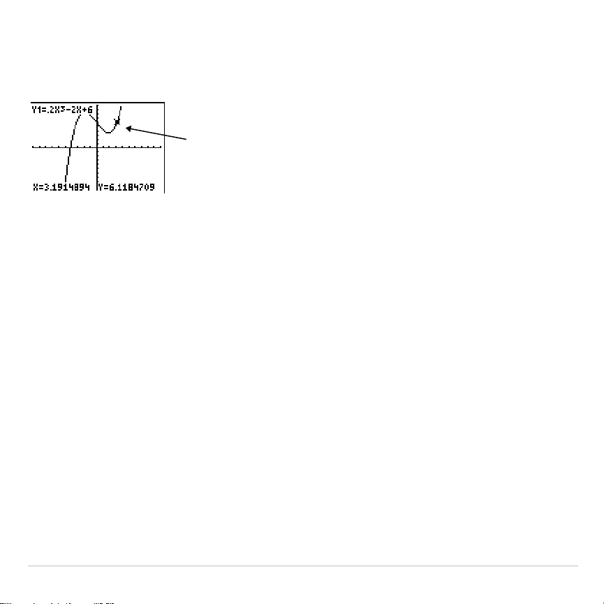
TI-83 Plus Function Graphing 135
When the trace cursor moves along a function, the
Y
value is calculated
from the
X
value; that is,
Y
=
Y
n
(X)
. If the function is undefined at an
X
value, the
Y
value is blank.
If you move the trace cursor beyond the top or bottom of the screen, the
coordinate values at the bottom of the screen continue to change
appropriately.
Moving the Trace Cursor from Function to Function
To move the trace cursor from function to function, press
†
and
}
. The
cursor follows the order of the selected functions in the
Y=
editor. The
trace cursor moves to each function at the same
X
value. If
ExprOn
format is selected, the expression is updated.
Moving the Trace Cursor to Any Valid X Value
To move the trace cursor to any valid
X
value on the current function,
enter the value. When you enter the first digit, an
X=
prompt and the
number you entered are displayed in the bottom-left corner of the
screen. You can enter an expression at the
X=
prompt. The value must
Trace cursor on the
curve
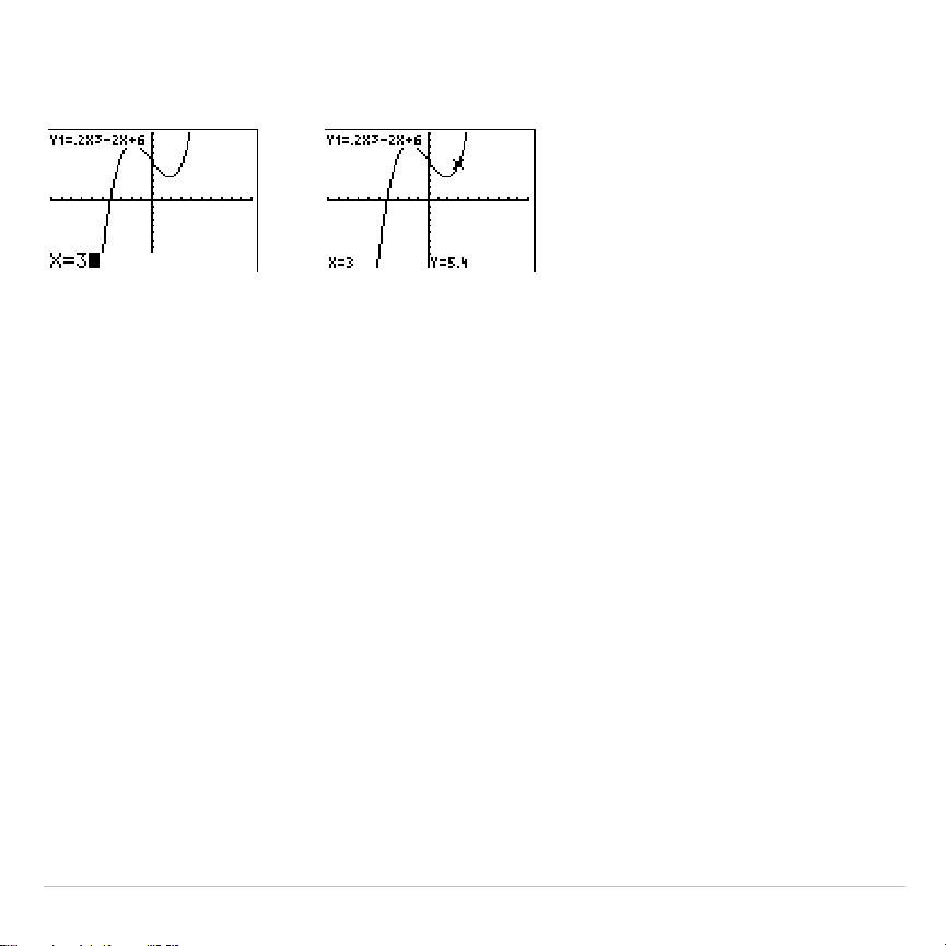
TI-83 Plus Function Graphing 136
be valid for the current viewing window. When you have completed the
entry, press
Í
to move the cursor.
Note:
This feature does not apply to stat plots.
Panning to the Left or Right
If you trace a function beyond the left or right side of the screen, the
viewing window automatically pans to the left or right.
Xmin
and
Xmax
are
updated to correspond to the new viewing window.
Quick Zoom
While tracing, you can press
Í
to adjust the viewing window so that
the cursor location becomes the center of the new viewing window, even
if the cursor is above or below the display. This allows panning up and
down. After Quick Zoom, the cursor remains in
TRACE
.

TI-83 Plus Function Graphing 137
Leaving and Returning to TRACE
When you leave and return to
TRACE
, the trace cursor is displayed in the
same location it was in when you left
TRACE
, unless Smart Graph has
replotted the graph.
Using TRACE in a Program
On a blank line in the program editor, press
r
. The instruction
Trace
is pasted to the cursor location. When the instruction is encountered
during program execution, the graph is displayed with the trace cursor on
the first selected function. As you trace, the cursor coordinate values are
updated. When you finish tracing the functions, press
Í
to resume
program execution.
TI-83 Plus Function Graphing 138
Exploring Graphs with the ZOOM
Instructions
ZOOM Menu
To display the
ZOOM
menu, press
q
. You can adjust the viewing
window of the graph quickly in several ways. All
ZOOM
instructions are
accessible from programs.
ZOOM MEMORY
1:ZBox
Draws a box to define the viewing window.
2:Zoom In
Magnifies the graph around the cursor.
3:Zoom Out
Views more of a graph around the cursor.
4:ZDecimal
Sets
@
X
and
@
Y
to 0.1.
5:ZSquare
Sets equal-size pixels on the
X
and
Y
axes.
6:ZStandard
Sets the standard window variables.
7:ZTrig
Sets the built-in trig window variables.
8:ZInteger
Sets integer values on the
X
and
Y
axes.
9:ZoomStat
Sets the values for current stat lists.
0:ZoomFit
Fits
YMin
and
YMax
between
XMin
and
XMax
.

TI-83 Plus Function Graphing 139
Zoom Cursor
When you select
1:ZBox
,
2:Zoom In
, or
3:Zoom Out
, the cursor on the
graph becomes the zoom cursor (
+
), a smaller version of the free-moving
cursor (
+
).
ZBox
To define a new viewing window using
ZBox
, follow these steps.
1. Select
1:ZBox
from the
ZOOM
menu. The zoom cursor is displayed at
the center of the screen.
2. Move the zoom cursor to any spot you want to define as a corner of
the box, and then press
Í
. When you move the cursor away from
the first defined corner, a small, square dot indicates the spot.
3. Press
|
,
}
,
~
, or
†
. As you move the cursor, the sides of the box
lengthen or shorten proportionately on the screen.
Note: To cancel
ZBox
before you press
Í
, press
‘
.
4. When you have defined the box, press
Í
to replot the graph.
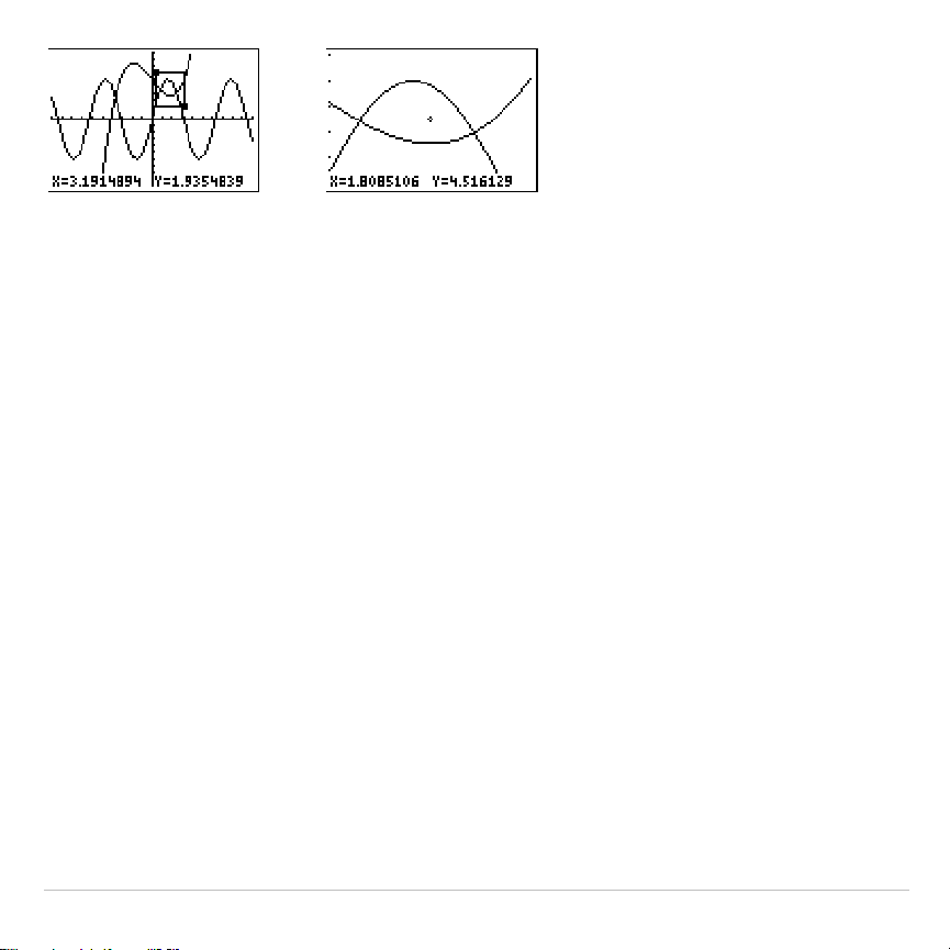
TI-83 Plus Function Graphing 140
To use
ZBox
to define another box within the new graph, repeat steps 2
through 4. To cancel
ZBox
, press
‘
.
Zoom In, Zoom Out
Zoom In
magnifies the part of the graph that surrounds the cursor
location.
Zoom Out
displays a greater portion of the graph, centered on
the cursor location. The
XFact
and
YFact
settings determine the extent of
the zoom.
To zoom in on a graph, follow these steps.
1. Check
XFact
and
YFact
; change as needed.
2. Select
2:Zoom In
from the
ZOOM
menu. The zoom cursor is displayed.
3. Move the zoom cursor to the point that is to be the center of the new
viewing window.

TI-83 Plus Function Graphing 141
4. Press
Í
. The TI-83 Plus adjusts the viewing window by
XFact
and
YFact
; updates the window variables; and replots the selected
functions, centered on the cursor location.
5. Zoom in on the graph again in either of two ways.
•
To zoom in at the same point, press
Í
.
•
To zoom in at a new point, move the cursor to the point that you
want as the center of the new viewing window, and then press
Í
.
To zoom out on a graph, select
3:Zoom Out
and repeat steps 3 through 5.
To cancel
Zoom In
or
Zoom Out
, press
‘
.
ZDecimal
ZDecimal
replots the functions immediately. It updates the window
variables to preset values, as shown below. These values set
@
X
and
@
Y
equal to
0.1
and set the
X
and
Y
value of each pixel to one decimal place.
Xmin=
L
4.7 Ymin=
L
3.1
Xmax=4.7 Ymax=3.1
Xscl=1 Yscl=1

TI-83 Plus Function Graphing 142
ZSquare
ZSquare
replots the functions immediately. It redefines the viewing
window based on the current values of the window variables. It adjusts in
only one direction so that
@
X=
@
Y
, which makes the graph of a circle look
like a circle.
Xscl
and
Yscl
remain unchanged. The midpoint of the
current graph (not the intersection of the axes) becomes the midpoint of
the new graph.
ZStandard
ZStandard
replots the functions immediately. It updates the window
variables to the standard values shown below.
Xmin=
L
10 Ymin=
L
10 Xres=1
Xmax=10 Ymax=10
Xscl=1 Yscl=1
ZTrig
ZTrig
replots the functions immediately. It updates the window variables
to preset values that are appropriate for plotting trig functions. Those
preset values in
Radian
mode are shown below.
Xmin=
L
(47
à
24)
p
Ymin=
L
4
Xmax=(47
à
24)
p
Ymax=4
Xscl=
p
/2 Yscl=1

TI-83 Plus Function Graphing 143
ZInteger
ZInteger
redefines the viewing window to the dimensions shown below.
To use
ZInteger
, move the cursor to the point that you want to be the
center of the new window, and then press
Í
;
ZInteger
replots the
functions.
@
X=1 Xscl=10
@
Y=1 Yscl=10
ZoomStat
ZoomStat
redefines the viewing window so that all statistical data points
are displayed. For regular and modified box plots, only
Xmin
and
Xmax
are adjusted.
ZoomFit
ZoomFit
replots the functions immediately.
ZoomFit
recalculates
YMin
and
YMax
to include the minimum and maximum
Y
values of the selected
functions between the current
XMin
and
XMax
.
XMin
and
XMax
are not
changed.
TI-83 Plus Function Graphing 144
Using ZOOM MEMORY
ZOOM MEMORY Menu
To display the
ZOOM MEMORY
menu, press
q
~
.
ZOOM MEMORY
1: ZPrevious
Uses the previous viewing window.
2: ZoomSto
Stores the user-defined window.
3: ZoomRcl
Recalls the user-defined window.
4: SetFactors
...
Changes
Zoom In
and
Zoom Out
factors.
ZPrevious
ZPrevious
replots the graph using the window variables of the graph that
was displayed before you executed the last
ZOOM
instruction.
ZoomSto
ZoomSto
immediately stores the current viewing window. The graph is
displayed, and the values of the current window variables are stored in
the user-defined
ZOOM
variables
ZXmin
,
ZXmax
,
ZXscl
,
ZYmin
,
ZYmax
,
ZYscl
, and
ZXres
.
These variables apply to all graphing modes. For example, changing the
value of
ZXmin
in
Func
mode also changes it in
Par
mode.
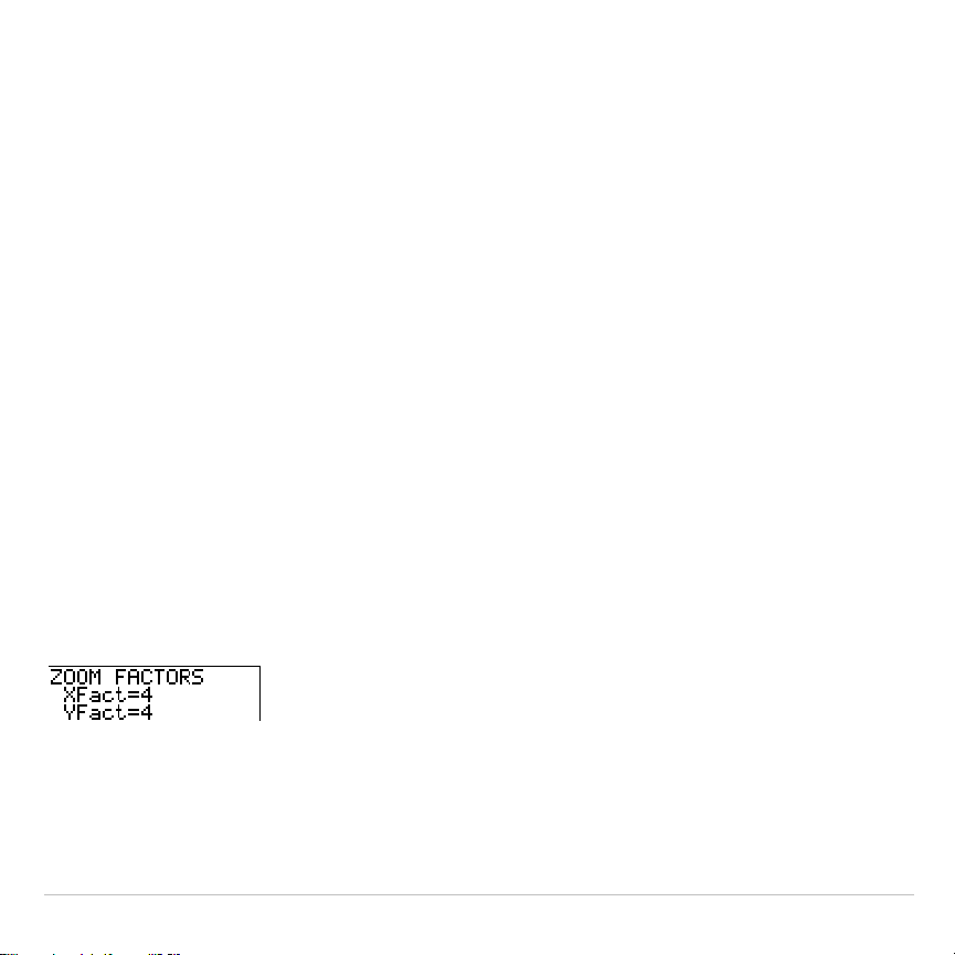
TI-83 Plus Function Graphing 145
ZoomRcl
ZoomRcl
graphs the selected functions in a user-defined viewing window.
The user-defined viewing window is determined by the values stored
with the
ZoomSto
instruction. The window variables are updated with the
user-defined values, and the graph is plotted.
ZOOM FACTORS
The zoom factors,
XFact
and
YFact
, are positive numbers (not
necessarily integers) greater than or equal to 1. They define the
magnification or reduction factor used to
Zoom In
or
Zoom Out
around a
point.
Checking XFact and YFact
To display the
ZOOM FACTORS
screen, where you can review the current
values for
XFact
and
YFact
, select
4:SetFactors
from the
ZOOM MEMORY
menu. The values shown are the defaults.

TI-83 Plus Function Graphing 146
Changing XFact and YFact
You can change
XFact
and
YFact
in either of two ways.
•
Enter a new value. The original value is cleared automatically when
you enter the first digit.
•
Place the cursor on the digit you want to change, and then enter a
value or press
{
to delete it.
Using ZOOM MEMORY Menu Items from the Home Screen or a
Program
From the home screen or a program, you can store directly to any of the
user-defined
ZOOM
variables.
From a program, you can select the
ZoomSto
and
ZoomRcl
instructions
from the
ZOOM MEMORY
menu.

TI-83 Plus Function Graphing 147
Using the CALC (Calculate) Operations
CALCULATE Menu
To display the
CALCULATE
menu, press
y
ã
CALCä
. Use the items on this
menu to analyze the current graph functions.
CALCULATE
1:value
Calculates a function
Y
value for a given
X
.
2:zero
Finds a zero (x-intercept) of a function.
3:minimum
Finds a minimum of a function.
4:maximum
Finds a maximum of a function.
5:intersect
Finds an intersection of two functions.
6:dy/dx
Finds a numeric derivative of a function.
7:
‰
f(x)dx
Finds a numeric integral of a function.
value
value
evaluates one or more currently selected functions for a specified
value of
X
.
Note: When a value is displayed for
X
, press
‘
to clear the value. When no
value is displayed, press
‘
to cancel the
value
operation.
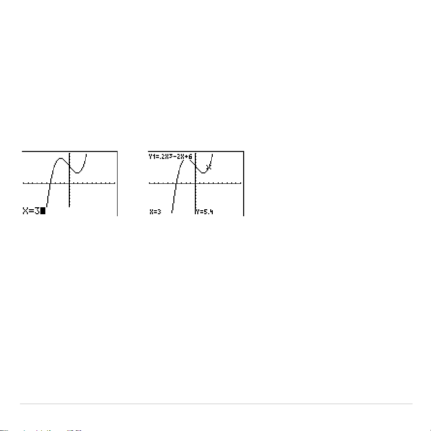
TI-83 Plus Function Graphing 148
To evaluate a selected function at
X
, follow these steps.
1. Select
1:value
from the
CALCULATE
menu. The graph is displayed with
X=
in the bottom-left corner.
2. Enter a real value, which can be an expression, for
X
between
Xmin
and
Xmax
.
3. Press
Í
.
The cursor is on the first selected function in the
Y=
editor at the
X
value
you entered, and the coordinates are displayed, even if
CoordOff
format
is selected.
To move the cursor from function to function at the entered
X
value,
press
}
or
†
. To restore the free-moving cursor, press
|
or
~
.
zero
zero
finds a zero (x-intercept or root) of a function using
solve(
. Functions
can have more than one x-intercept value;
zero
finds the zero closest to
your guess.
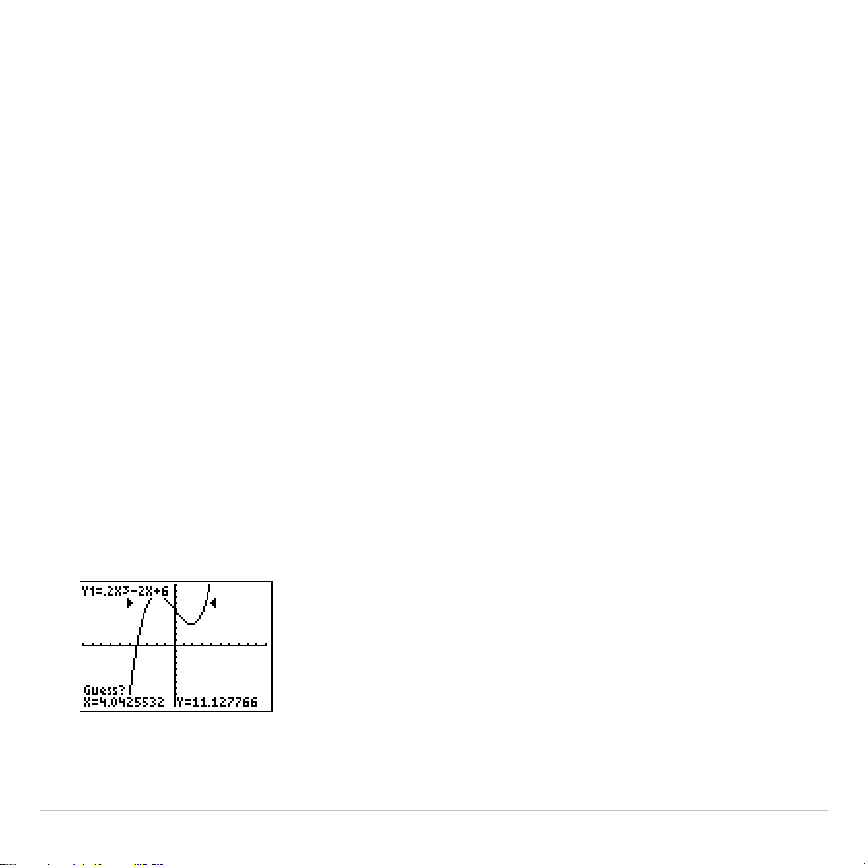
TI-83 Plus Function Graphing 149
The time
zero
spends to find the correct zero value depends on the
accuracy of the values you specify for the left and right bounds and the
accuracy of your guess.
To find a zero of a function, follow these steps.
1. Select
2:zero
from the
CALCULATE
menu. The current graph is
displayed with
Left Bound?
in the bottom-left corner.
2. Press
}
or
†
to move the cursor onto the function for which you
want to find a zero.
3. Press
|
or
~
(or enter a value) to select the x-value for the left
bound of the interval, and then press
Í
. A
4
indicator on the
graph screen shows the left bound.
Right Bound?
is displayed in the
bottom-left corner. Press
|
or
~
(or enter a value) to select the
x-value for the right bound, and then press
Í
. A
3
indicator on the
graph screen shows the right bound.
Guess?
is then displayed in the
bottom-left corner.
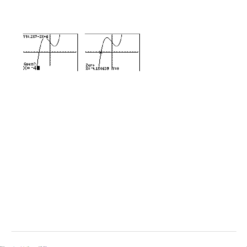
TI-83 Plus Function Graphing 150
4. Press
|
or
~
(or enter a value) to select a point near the zero of the
function, between the bounds, and then press
Í
.
The cursor is on the solution and the coordinates are displayed, even if
CoordOff
format is selected. To move to the same x-value for other
selected functions, press
}
or
†
. To restore the free-moving cursor,
press
|
or
~
.
minimum, maximum
minimum
and
maximum
find a minimum or maximum of a function within
a specified interval to a tolerance of 1
â
L
5.
To find a minimum or maximum, follow these steps.
1. Select
3:minimum
or
4:maximum
from the
CALCULATE
menu. The
current graph is displayed.
2. Select the function and set left bound, right bound, and guess as
described for
zero
.
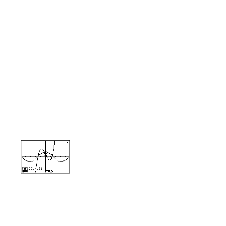
TI-83 Plus Function Graphing 151
The cursor is on the solution, and the coordinates are displayed, even if
you have selected
CoordOff
format;
Minimum
or
Maximum
is displayed in
the bottom-left corner.
To move to the same x-value for other selected functions, press
}
or
†
.
To restore the free-moving cursor, press
|
or
~
.
intersect
intersect
finds the coordinates of a point at which two or more functions
intersect using
solve(
. The intersection must appear on the display to use
intersect
.
To find an intersection, follow these steps.
1. Select
5:intersect
from the
CALCULATE
menu. The current graph is
displayed with
First curve?
in the bottom-left corner.
2. Press
†
or
}
, if necessary, to move the cursor to the first function,
and then press
Í
.
Second curve?
is displayed in the bottom-left
corner.

TI-83 Plus Function Graphing 152
3. Press
†
or
}
, if necessary, to move the cursor to the second
function, and then press
Í
.
4. Press
~
or
|
to move the cursor to the point that is your guess as to
location of the intersection, and then press
Í
.
The cursor is on the solution and the coordinates are displayed, even if
CoordOff
format is selected.
Intersection
is displayed in the bottom-left
corner. To restore the free-moving cursor, press
|
,
}
,
~
, or
†
.
dy/dx
dy/dx
(numerical derivative) finds the numerical derivative (slope) of a
function at a point, with
H
=1
â
L
3.
To find a function’s slope at a point, follow these steps.
1. Select
6:dy/dx
from the
CALCULATE
menu. The current graph is
displayed.
2. Press
}
or
†
to select the function for which you want to find the
numerical derivative.
3. Press
|
or
~
(or enter a value) to select the
X
value at which to
calculate the derivative, and then press
Í
.
The cursor is on the solution and the numerical derivative is displayed.
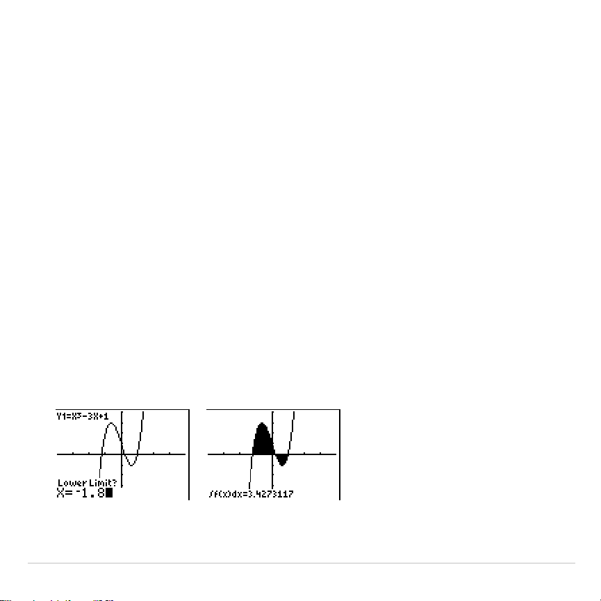
TI-83 Plus Function Graphing 153
To move to the same x-value for other selected functions, press
}
or
†
.
To restore the free-moving cursor, press
|
or
~
.
‰
f(x)dx
‰
f(x)dx
(numerical integral) finds the numerical integral of a function in a
specified interval. It uses the
fnInt(
function, with a tolerance of
H
=1
â
L
3.
To find the numerical derivative of a function, follow these steps.
1. Select
7:
‰
f(x)dx
from the
CALCULATE
menu. The current graph is
displayed with
Lower Limit?
in the bottom-left corner.
2. Press
}
or
†
to move the cursor to the function for which you want
to calculate the integral.
3. Set lower and upper limits as you would set left and right bounds for
zero
. The integral value is displayed, and the integrated area is
shaded.
Note: The shaded area is a drawing. Use
ClrDraw
(Chapter 8) or any action
that invokes Smart Graph to clear the shaded area.

TI-83 Plus Parametric Graphing 154
Chapter 4:
Parametric Graphing
Getting Started: Path of a Ball
Getting Started is a fast-paced introduction. Read the chapter for details.
Graph the parametric equation that describes the path of a ball hit at an initial
speed of 30 meters per second, at an initial angle of 25 degrees with the
horizontal from ground level. How far does the ball travel? When does it hit the
ground? How high does it go? Ignore all forces except gravity.
For initial velocity v
0
and angle
q
, the position of the ball as a function of time has
horizontal and vertical components.
Horizontal: X1(t)=tv
0
cos(
q
) Vertical: Y1(t)=tv
0
sin(
q
)
N
1
2
gt
2
The vertical and horizontal vectors of the ball’s motion also will be graphed.
Vertical vector: X2(t)=0 Y2(t)=Y1(t)
Horizontal vector: X3(t)=X1(t) Y3(t)=0
Gravity constant: g=9.8 m/sec
2
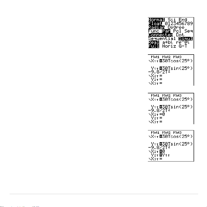
TI-83 Plus Parametric Graphing 155
1. Press
z
. Press
†
†
†
~
Í
to select
Par
mode. Press
†
†
~
Í
to select
Simul
for simultaneous graphing of all three
parametric equations in this example.
2. Press
o
. Press
30
„
™
25
y
;
1
(to select
¡
)
¤
Í
to define
X
1T
in terms of
T
.
3. Press
30
„
˜
25
y
;
1
¤
¹
9.8
¥
2
„
¡
Í
to define
Y
1T
.
The vertical component vector is defined by
X
2T
and
Y
2T
.
4. Press
0
Í
to define
X
2T
.
5. Press
~
to display the
VARS Y
.
VARS
menu.
Press
2
to display the
PARAMETRIC
secondary
menu. Press
2
Í
to define
Y
2T
.
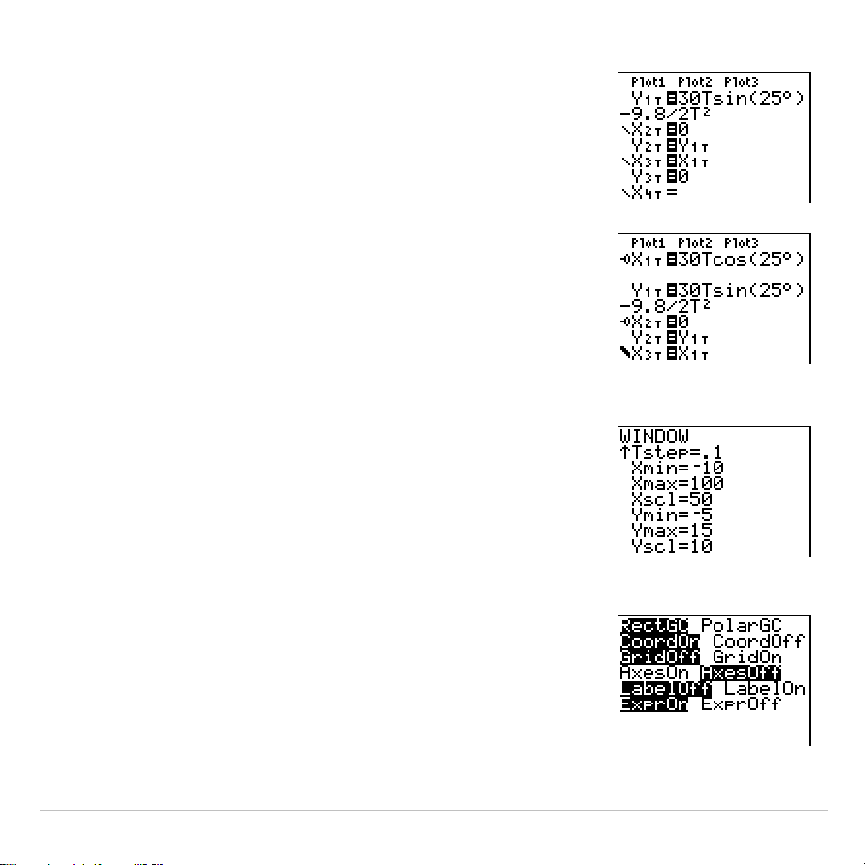
TI-83 Plus Parametric Graphing 156
The horizontal component vector is defined by
X
3T
and
Y
3T
.
6. Press
~
2
, and then press
1
Í
to
define
X
3T
. Press
0
Í
to define
Y
3T
.
7. Press
|
|
}
Í
to change the graph style
to
è
for
X
3T
and
Y
3T
. Press
}
Í
Í
to
change the graph style to
ë
for
X
2T
and
Y
2T
.
Press
}
Í
Í
to change the graph style
to
ë
for
X
1T
and
Y
1T
. (These keystrokes assume
that all graph styles were set to
ç
originally.)
8. Press
p
. Enter these values for the
window variables.
Tmin=0 Xmin=
L
10 Ymin=
L
5
Tmax=5 Xmax=100 Ymax=15
Tstep=.1 Xscl=50 Yscl=10
9. Press
y
.
†
†
†
~
Í
to set
AxesOff
, which turns off the axes.
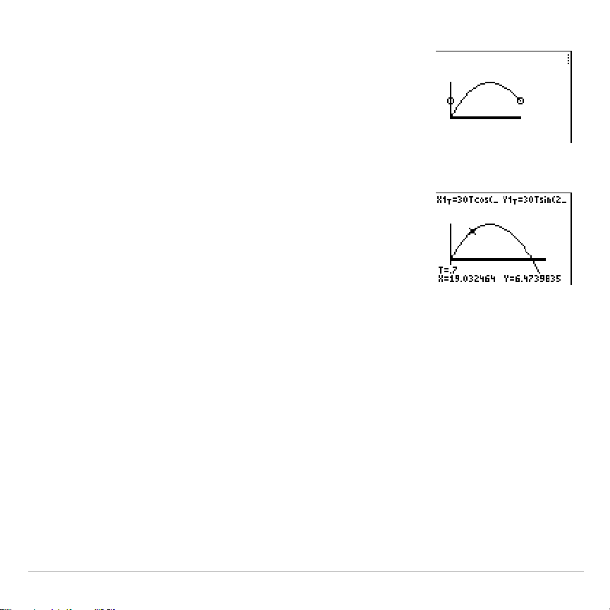
TI-83 Plus Parametric Graphing 157
10.Press
s
. The plotting action
simultaneously shows the ball in flight and the
vertical and horizontal component vectors of the
motion.
Tip:
To simulate the ball flying through the air, set
graph style to
ì
(animate) for
X
1T
and
Y
1T
.
11.Press
r
to obtain numerical results and
answer the questions at the beginning of this
section.
Tracing begins at
Tmin
on the first parametric
equation (
X
1T
and
Y
1T
). As you press
~
to trace
the curve, the cursor follows the path of the ball
over time. The values for
X
(distance),
Y
(height), and
T
(time) are displayed at the
bottom of the screen.
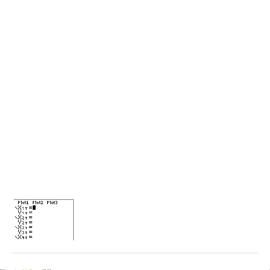
TI-83 Plus Parametric Graphing 158
Defining and Displaying Parametric Graphs
TI-83 Plus Graphing Mode Similarities
The steps for defining a parametric graph are similar to the steps for
defining a function graph. Chapter 4 assumes that you are familiar with
Chapter 3: Function Graphing. Chapter 4 details aspects of parametric
graphing that differ from function graphing.
Setting Parametric Graphing Mode
To display the mode screen, press
z
. To graph parametric equations,
you must select
Par
graphing mode before you enter window variables
and before you enter the components of parametric equations.
Displaying the Parametric Y= Editor
After selecting
Par
graphing mode, press
o
to display the parametric
Y=
editor.

TI-83 Plus Parametric Graphing 159
In this editor, you can display and enter both the
X
and
Y
components of
up to six equations,
X
1T
and
Y
1T
through
X
6T
and
Y
6T
. Each is defined in
terms of the independent variable
T
. A common application of parametric
graphs is graphing equations over time.
Selecting a Graph Style
The icons to the left of
X
1T
through
X
6T
represent the graph style of each
parametric equation (Chapter 3). The default in
Par
mode is
ç
(line),
which connects plotted points. Line,
è
(thick),
ë
(path),
ì
(animate), and
í
(dot) styles are available for parametric graphing.
Defining and Editing Parametric Equations
To define or edit a parametric equation, follow the steps in Chapter 3 for
defining a function or editing a function. The independent variable in a
parametric equation is
T
. In
Par
graphing mode, you can enter the
parametric variable
T
in either of two ways.
•
Press
„
.
•
Press
ƒ
ã
Tä
.
Two components,
X
and
Y
, define a single parametric equation. You
must define both of them.

TI-83 Plus Parametric Graphing 160
Selecting and Deselecting Parametric Equations
The TI-83 Plus graphs only the selected parametric equations. In the
Y=
editor, a parametric equation is selected when the
=
signs of both the
X
and
Y
components are highlighted. You may select any or all of the
equations
X
1T
and
Y
1T
through
X
6T
and
Y
6T
.
To change the selection status, move the cursor onto the
=
sign of either
the
X
or
Y
component and press
Í
. The status of both the
X
and
Y
components is changed.
Setting Window Variables
To display the window variable values, press
p
. These variables
define the viewing window. The values below are defaults for
Par
graphing in
Radian
angle mode.
Tmin=0
Smallest T value to evaluate
Tmax=6.2831853
...
Largest T value to evaluate (2
p
)
Tstep=.1308996
...
T value increment (
pà
24)
Xmin=
L
10
Smallest X value to be displayed
Xmax=10
Largest X value to be displayed
Xscl=1
Spacing between the X tick marks
Ymin=
L
10
Smallest Y value to be displayed
Ymax=10
Largest Y value to be displayed
Yscl=1
Spacing between the Y tick marks
Note: To ensure that sufficient points are plotted, you may want to change the
T
window variables.
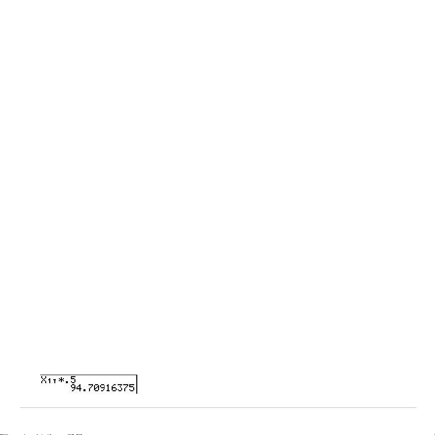
TI-83 Plus Parametric Graphing 161
Setting the Graph Format
To display the current graph format settings, press
y
.
. Chapter
3 describes the format settings in detail. The other graphing modes
share these format settings;
Seq
graphing mode has an additional axes
format setting.
Displaying a Graph
When you press
s
, the TI-83 Plus plots the selected parametric
equations. It evaluates the
X
and
Y
components for each value of
T
(from
Tmin
to
Tmax
in intervals of
Tstep
), and then plots each point defined by
X
and
Y
. The window variables define the viewing window.
As the graph is plotted,
X
,
Y
, and
T
are updated.
Smart Graph applies to parametric graphs (Chapter 3).
Window Variables and Y
.
VARS Menus
You can perform these actions from the home screen or a program.
•
Access functions by using the name of the
X
or
Y
component of the
equation as a variable.
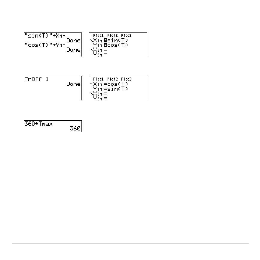
TI-83 Plus Parametric Graphing 162
•
Store parametric equations.
•
Select or deselect parametric equations.
•
Store values directly to window variables.

TI-83 Plus Parametric Graphing 163
Exploring Parametric Graphs
Free-Moving Cursor
The free-moving cursor in
Par
graphing works the same as in
Func
graphing.
In
RectGC
format, moving the cursor updates the values of
X
and
Y
; if
CoordOn
format is selected,
X
and
Y
are displayed.
In
PolarGC
format,
X
,
Y
,
R
, and
q
are updated; if
CoordOn
format is
selected,
R
and
q
are displayed.
TRACE
To activate
TRACE
, press
r
. When
TRACE
is active, you can move the
trace cursor along the graph of the equation one
Tstep
at a time. When
you begin a trace, the trace cursor is on the first selected function at
Tmin
. If
ExprOn
is selected, then the function is displayed.
In
RectGC
format,
TRACE
updates and displays the values of
X
,
Y
, and
T
if
CoordOn
format is on.
In
PolarGC
format,
X
,
Y
,
R
,
q
and
T
are updated; if
CoordOn
format is
selected,
R
,
q
, and
T
are displayed. The
X
and
Y
(or
R
and
q
) values are
calculated from
T
.
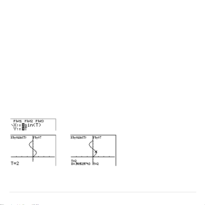
TI-83 Plus Parametric Graphing 164
To move five plotted points at a time on a function, press
y
|
or
y
~
. If you move the cursor beyond the top or bottom of the screen,
the coordinate values at the bottom of the screen continue to change
appropriately.
Quick Zoom is available in
Par
graphing; panning is not (Chapter 3).
Moving the Trace Cursor to Any Valid T Value
To move the trace cursor to any valid
T
value on the current function,
enter the number. When you enter the first digit, a
T=
prompt and the
number you entered are displayed in the bottom-left corner of the
screen. You can enter an expression at the
T=
prompt. The value must
be valid for the current viewing window. When you have completed the
entry, press
Í
to move the cursor.

TI-83 Plus Parametric Graphing 165
ZOOM
ZOOM
operations in
Par
graphing work the same as in
Func
graphing.
Only the
X
(
Xmin
,
Xmax
, and
Xscl
) and
Y
(
Ymin
,
Ymax
, and
Yscl
) window
variables are affected.
The
T
window variables (
Tmin
,
Tmax
, and
Tstep
) are only affected when
you select
ZStandard
. The
VARS ZOOM
secondary menu
ZT/Z
q
items
1:ZTmin
,
2:ZTmax
, and
3:ZTstep
are the zoom memory variables for
Par
graphing.
CALC
CALC
operations in
Par
graphing work the same as in
Func
graphing. The
CALCULATE
menu items available in
Par
graphing are
1:value
,
2:dy/dx
,
3:dy/dt
, and
4:dx/dt
.
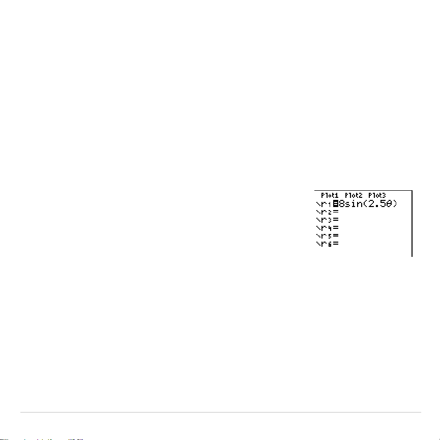
TI-83 Plus Polar Graphing 166
Chapter 5:
Polar Graphing
Getting Started: Polar Rose
Getting Started is a fast-paced introduction. Read the chapter for details.
The polar equation R=Asin(B
q
) graphs a rose. Graph the rose for A=8 and B=2.5,
and then explore the appearance of the rose for other values of A and B.
1. Press
z
to display the mode screen. Press
†
†
†
~
~
Í
to select
Pol
graphing
mode. Select the defaults (the options on the
left) for the other mode settings.
2. Press
o
to display the polar
Y=
editor. Press
8
˜
2.5
„
¤
Í
to define
r
1
.
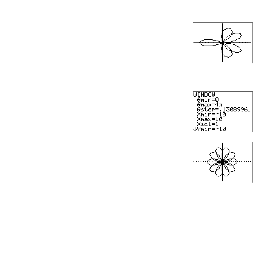
TI-83 Plus Polar Graphing 167
3. Press
q
6
to select
6:ZStandard
and graph
the equation in the standard viewing window.
The graph shows only five petals of the rose,
and the rose does not appear to be
symmetrical. This is because the standard
window sets
q
max=2
p
and defines the window,
rather than the pixels, as square.
4. Press
p
to display the window variables.
Press
†
4
y
B
to increase the value of
q
max
to 4
p
.
5. Press
q
5
to select
5:ZSquare
and plot the
graph.
6. Repeat steps 2 through 5 with new values for
the variables
A
and
B
in the polar equation
r1=Asin(B
q
)
. Observe how the new values affect
the graph.
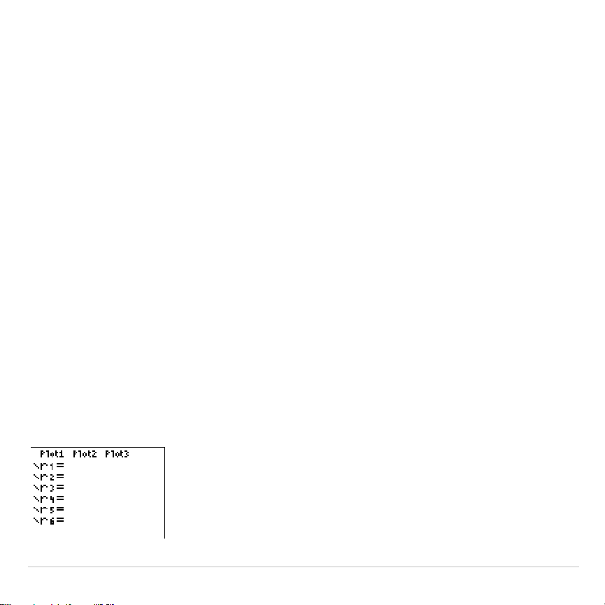
TI-83 Plus Polar Graphing 168
Defining and Displaying Polar Graphs
TI-83 Plus Graphing Mode Similarities
The steps for defining a polar graph are similar to the steps for defining a
function graph. Chapter 5 assumes that you are familiar with Chapter 3:
Function Graphing. Chapter 5 details aspects of polar graphing that differ
from function graphing.
Setting Polar Graphing Mode
To display the mode screen, press
z
. To graph polar equations, you
must select
Pol
graphing mode before you enter values for the window
variables and before you enter polar equations.
Displaying the Polar Y= Editor
After selecting
Pol
graphing mode, press
o
to display the polar
Y=
editor.

TI-83 Plus Polar Graphing 169
In this editor, you can enter and display up to six polar equations,
r1
through
r6
. Each is defined in terms of the independent variable
q
.
Selecting Graph Styles
The icons to the left of
r1
through
r6
represent the graph style of each
polar equation (Chapter 3). The default in
Pol
graphing mode is
ç
(line),
which connects plotted points. Line,
è
(thick),
ë
(path),
ì
(animate), and
í
(dot) styles are available for polar graphing.
Defining and Editing Polar Equations
To define or edit a polar equation, follow the steps in Chapter 3 for
defining a function or editing a function. The independent variable in a
polar equation is
q
. In
Pol
graphing mode, you can enter the polar
variable
q
in either of two ways.
•
Press
„
.
•
Press
ƒ
ãqä
.
Selecting and Deselecting Polar Equations
The TI-83 Plus graphs only the selected polar equations. In the
Y=
editor,
a polar equation is selected when the
=
sign is highlighted. You may
select any or all of the equations.

TI-83 Plus Polar Graphing 170
To change the selection status, move the cursor onto the
=
sign, and
then press
Í
.
Setting Window Variables
To display the window variable values, press
p
. These variables
define the viewing window. The values below are defaults for
Pol
graphing in
Radian
angle mode.
q
min=0
Smallest
q
value to evaluate
q
max=6.2831853
...
Largest
q
value to evaluate (2
p
)
q
step=.1308996
...
Increment between
q
values (
pà
24)
Xmin=
L
10
Smallest
X
value to be displayed
Xmax=10
Largest
X
value to be displayed
Xscl=1
Spacing between the
X
tick marks
Ymin=
L
10
Smallest
Y
value to be displayed
Ymax=10
Largest
Y
value to be displayed
Yscl=1
Spacing between the
Y
tick marks
Note: To ensure that sufficient points are plotted, you may want to change the
q
window variables.
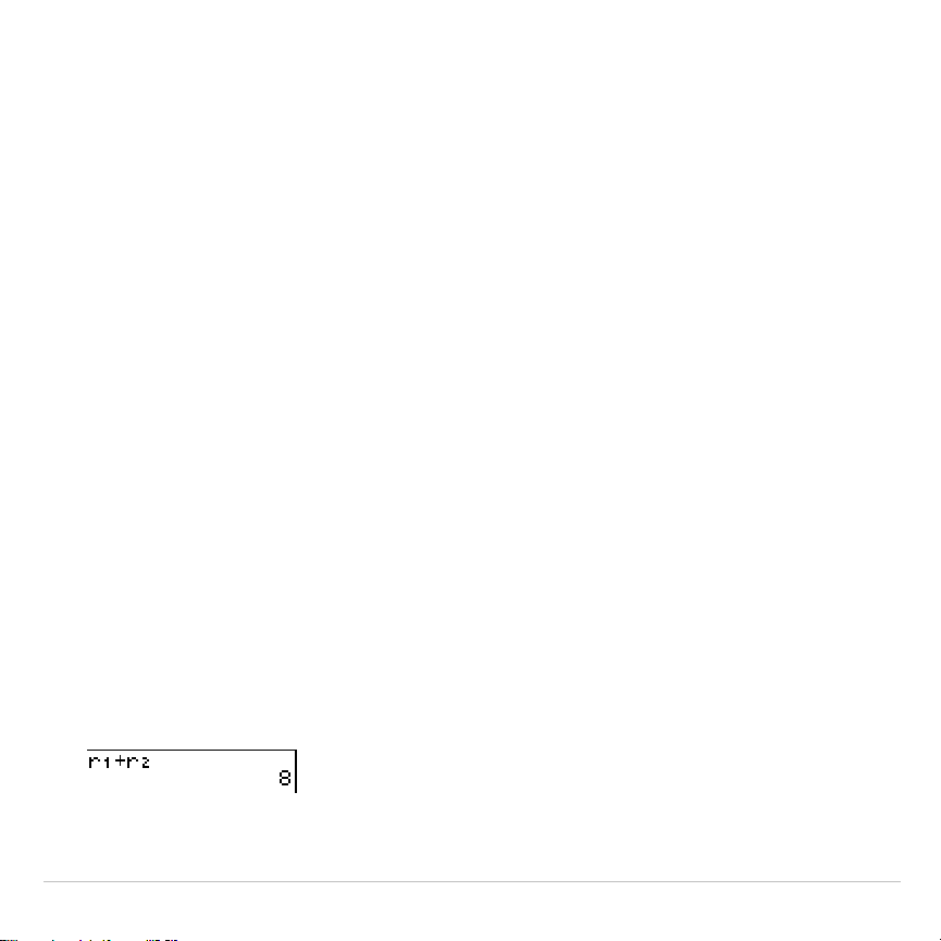
TI-83 Plus Polar Graphing 171
Setting the Graph Format
To display the current graph format settings, press
y
.
. Chapter
3 describes the format settings in detail. The other graphing modes
share these format settings.
Displaying a Graph
When you press
s
, the TI-83 Plus plots the selected polar
equations. It evaluates
R
for each value of
q
(from
q
min
to
q
max
in
intervals of
q
step
) and then plots each point. The window variables define
the viewing window.
As the graph is plotted,
X
,
Y
,
R
, and
q
are updated.
Smart Graph applies to polar graphs (Chapter 3).
Window Variables and Y
.
VARS Menus
You can perform these actions from the home screen or a program.
•
Access functions by using the name of the equation as a variable.
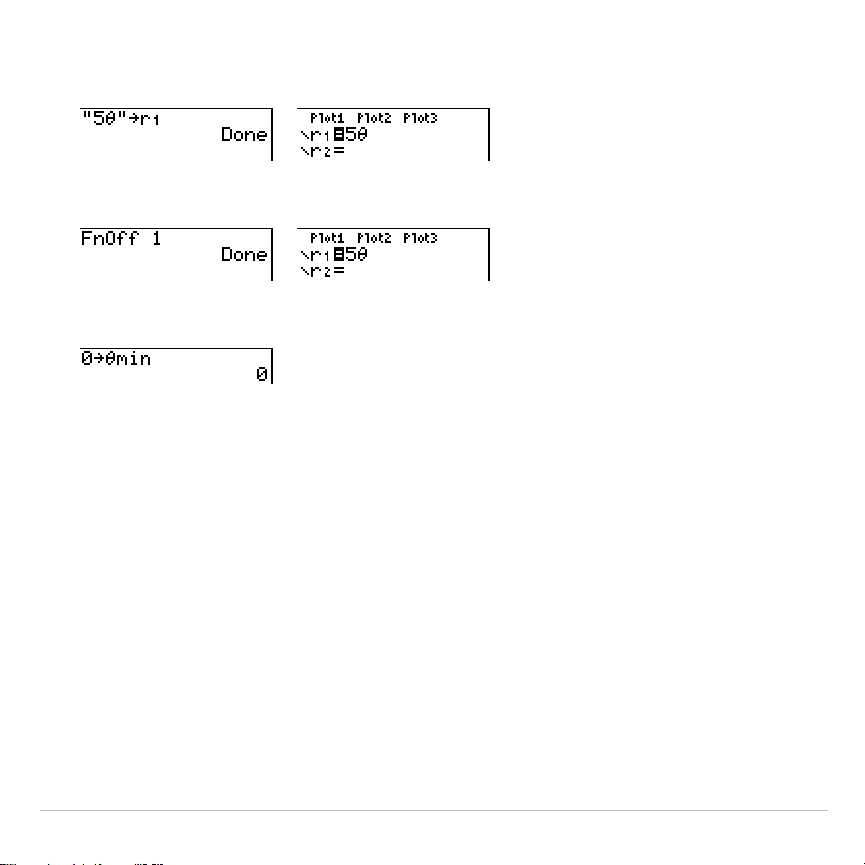
TI-83 Plus Polar Graphing 172
•
Store polar equations.
•
Select or deselect polar equations.
•
Store values directly to window variables.

TI-83 Plus Polar Graphing 173
Exploring Polar Graphs
Free-Moving Cursor
The free-moving cursor in
Pol
graphing works the same as in
Func
graphing. In
RectGC
format, moving the cursor updates the values of
X
and
Y
; if
CoordOn
format is selected,
X
and
Y
are displayed. In
PolarGC
format,
X
,
Y
,
R
, and
q
are updated; if
CoordOn
format is selected,
R
and
q
are displayed.
TRACE
To activate
TRACE
, press
r
. When
TRACE
is active, you can move the
trace cursor along the graph of the equation one
q
step
at a time. When
you begin a trace, the trace cursor is on the first selected function at
q
min
. If
ExprOn
format is selected, then the equation is displayed.
In
RectGC
format,
TRACE
updates the values of
X
,
Y
, and
q
; if
CoordOn
format is selected,
X
,
Y
, and
q
are displayed. In
PolarGC
format,
TRACE
updates
X
,
Y
,
R
, and
q
; if
CoordOn
format is selected,
R
and
q
are
displayed.
To move five plotted points at a time on a function, press
y
|
or
y
~
. If you move the trace cursor beyond the top or bottom of the

TI-83 Plus Polar Graphing 174
screen, the coordinate values at the bottom of the screen continue to
change appropriately.
Quick Zoom is available in
Pol
graphing mode; panning is not (Chapter 3).
Moving the Trace Cursor to Any Valid
q
Value
To move the trace cursor to any valid
q
value on the current function,
enter the number. When you enter the first digit, a
q
=
prompt and the
number you entered are displayed in the bottom-left corner of the
screen. You can enter an expression at the
q
=
prompt. The value must
be valid for the current viewing window. When you complete the entry,
press
Í
to move the cursor.
ZOOM
ZOOM
operations in
Pol
graphing work the same as in
Func
graphing.
Only the
X
(
Xmin
,
Xmax
, and
Xscl
) and
Y
(
Ymin
,
Ymax
, and
Yscl
) window
variables are affected.
The
q
window variables (
q
min
,
q
max
, and
q
step
) are not affected, except
when you select
ZStandard
. The
VARS ZOOM
secondary menu
ZT/Z
q
items
4:Z
q
min
,
5:Z
q
max
, and
6:Z
q
step
are zoom memory variables for
Pol
graphing.

TI-83 Plus Polar Graphing 175
CALC
CALC
operations in
Pol
graphing work the same as in
Func
graphing. The
CALCULATE
menu items available in
Pol
graphing are
1:value
,
2:dy/dx
, and
3:dr/d
q
.
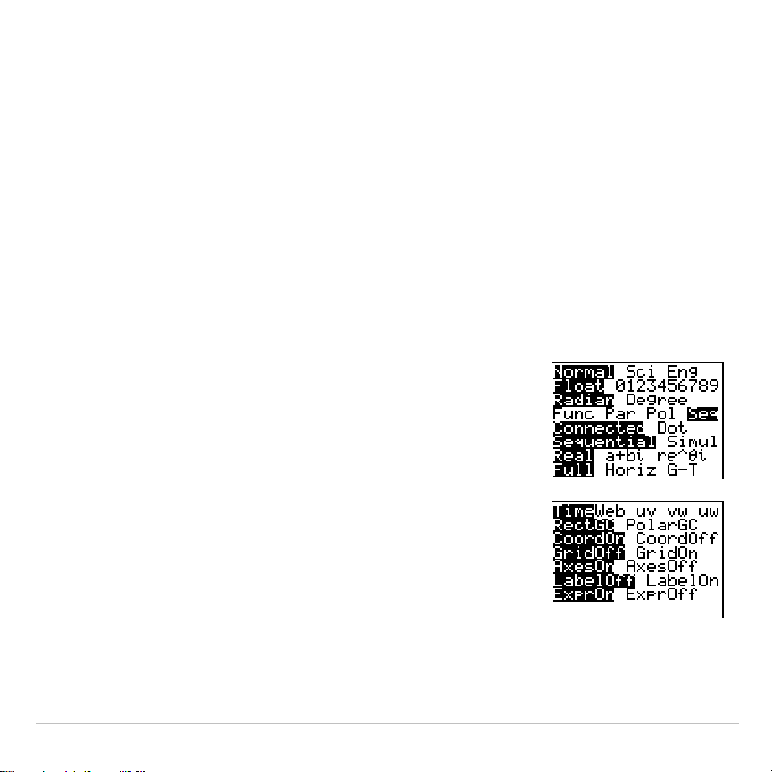
TI-83 Plus Sequence Graphing 176
Chapter 6:
Sequence Graphing
Getting Started: Forest and Trees
Getting Started is a fast-paced introduction. Read the chapter for details.
A small forest of 4,000 trees is under a new forestry plan. Each year 20 percent of
the trees will be harvested and 1,000 new trees will be planted. Will the forest
eventually disappear? Will the forest size stabilize? If so, in how many years and
with how many trees?
1. Press
z
. Press
†
†
†
~
~
~
Í
to
select
Seq
graphing mode.
2. Press
y
.
and select
Time
axes format
and
ExprOn
format if necessary.
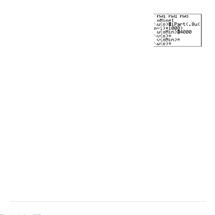
TI-83 Plus Sequence Graphing 177
3. Press
o
. If the graph-style icon is not
í
(dot),
press
|
|
, press
Í
until
í
is displayed,
and then press
~
~
.
4. Press
~
3
to select
iPart(
(integer part)
because only whole trees are harvested. After
each annual harvest, 80 percent (.80) of the
trees remain.
Press
Ë
8
y
[
u
]
£
„
¹
1
¤
to define
the number of trees after each harvest. Press
Ã
1000
¤
to define the new trees. Press
†
4000
to define the number of trees at the
beginning of the program.
5. Press
p
0
to set
n
Min=0
. Press
†
50
to
set
n
Max=50
.
n
Min
and
n
Max
evaluate forest
size over 50 years. Set the other window
variables.
PlotStart=1 Xmin=0 Ymin=0
PlotStep=1 Xmax=50 Ymax=6000
Xscl=10 Yscl=1000
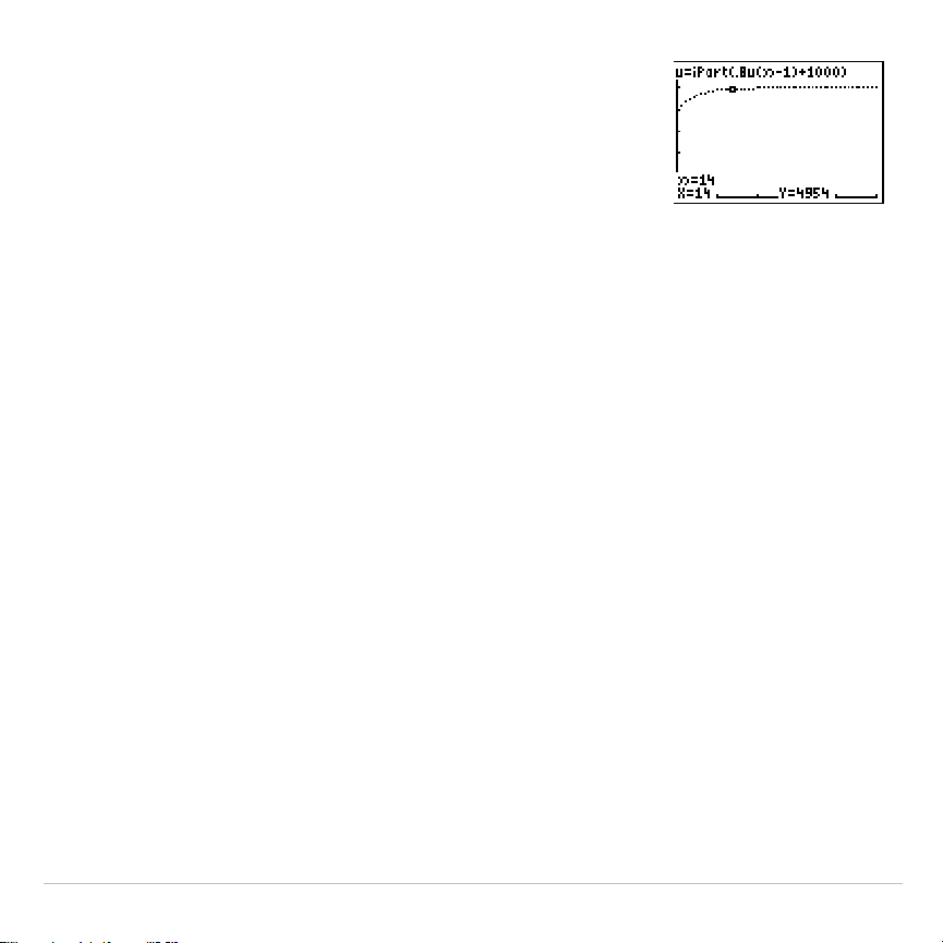
TI-83 Plus Sequence Graphing 178
6. Press
r
. Tracing begins at
n
Min
(the start
of the forestry plan). Press
~
to trace the
sequence year by year. The sequence is
displayed at the top of the screen. The values
for
n
(number of years),
X
(
X=
n
, because
n
is
plotted on the x-axis), and
Y
(tree count) are
displayed at the bottom. When will the forest
stabilize? With how many trees?

TI-83 Plus Sequence Graphing 179
Defining and Displaying Sequence Graphs
TI-83 Plus Graphing Mode Similarities
The steps for defining a sequence graph are similar to the steps for
defining a function graph. Chapter 6 assumes that you are familiar with
Chapter 3: Function Graphing. Chapter 6 details aspects of sequence
graphing that differ from function graphing.
Setting Sequence Graphing Mode
To display the mode screen, press
z
. To graph sequence functions,
you must select
Seq
graphing mode before you enter window variables
and before you enter sequence functions.
Sequence graphs automatically plot in
Simul
mode, regardless of the
current plotting-order mode setting.
TI-83 Plus Sequence Functions u, v, and w
The TI-83 Plus has three sequence functions that you can enter from the
keyboard:
u
,
v
, and
w
. They are above the
¬
,
−
, and
®
keys.
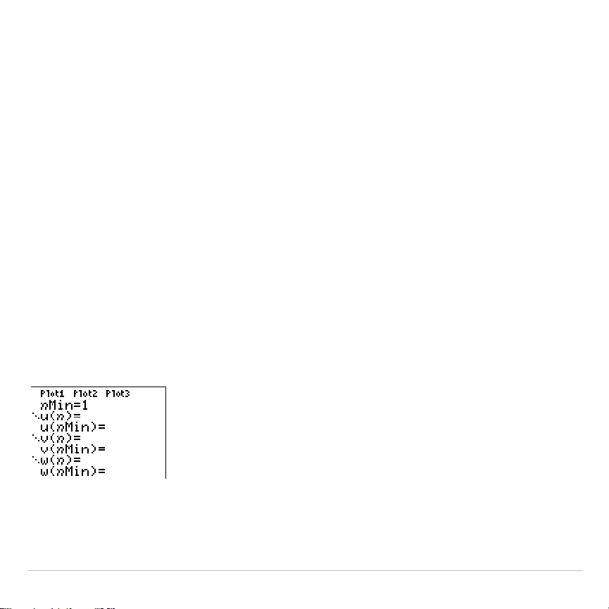
TI-83 Plus Sequence Graphing 180
You can define sequence functions in terms of:
•
The independent variable
n
•
The previous term in the sequence function, such as
u(
n
N
1)
•
The term that precedes the previous term in the sequence function,
such as
u(
n
N
2)
•
The previous term or the term that precedes the previous term in
another sequence function, such as
u(
n
N
1)
or
u(
n
N
2)
referenced in the
sequence
v(
n
)
.
Note: Statements in this chapter about
u(
n
)
are also true for
v(
n
)
and
w(
n
)
;
statements about
u(
n
N
1)
are also true for
v(
n
N
1)
and
w(
n
N
1)
; statements about
u(
n
N
2)
are also true for
v(
n
N
2)
and
w(
n
N
2)
.
Displaying the Sequence Y= Editor
After selecting
Seq
mode, press
o
to display the sequence
Y=
editor.
In this editor, you can display and enter sequences for
u(
n
)
,
v(
n
)
, and
w(
n
)
. Also, you can edit the value for
n
Min
, which is the sequence
window variable that defines the minimum
n
value to evaluate.

TI-83 Plus Sequence Graphing 181
The sequence
Y=
editor displays the
n
Min
value because of its relevance
to
u(
n
Min)
,
v(
n
Min)
, and
w(
n
Min)
, which are the initial values for the
sequence equations
u(
n
)
,
v(
n
)
, and
w(
n
)
, respectively.
n
Min
in the
Y=
editor is the same as
n
Min
in the window editor. If you
enter a new value for
n
Min
in one editor, the new value for
n
Min
is
updated in both editors.
Note: Use
u(
n
Min)
,
v(
n
Min)
, or
w(
n
Min)
only with a recursive sequence, which
requires an initial value.
Selecting Graph Styles
The icons to the left of
u(
n
)
,
v(
n
)
, and
w(
n
)
represent the graph style of
each sequence (Chapter 3). The default in
Seq
mode is
í
(dot), which
shows discrete values. Dot,
ç
(line), and
è
(thick) styles are available for
sequence graphing. Graph styles are ignored in
Web
format.
Selecting and Deselecting Sequence Functions
The TI-83 Plus graphs only the selected sequence functions. In the
Y=
editor, a sequence function is selected when the
=
signs of both
u(
n
)=
and
u(
n
Min)=
are highlighted.
To change the selection status of a sequence function, move the cursor
onto the
=
sign of the function name, and then press
Í
. The status is
changed for both the sequence function
u(
n
)
and its initial value
u(
n
Min)
.

TI-83 Plus Sequence Graphing 182
Defining and Editing a Sequence Function
To define or edit a sequence function, follow the steps in Chapter 3 for
defining a function. The independent variable in a sequence is
n
.
In
Seq
graphing mode, you can enter the sequence variable in either of
two ways.
•
Press
„
.
•
Press
y
N
[
N
].
You can enter the function name from the keyboard.
•
To enter the function name
u
, press
y
[
u
] (above
¬
).
•
To enter the function name
v
, press
y
[
v
] (above
−
).
•
To enter the function name
w
, press
y
[
w
] (above
®
).
Generally, sequences are either nonrecursive or recursive. Sequences
are evaluated only at consecutive integer values.
n
is always a series of
consecutive integers, starting at zero or any positive integer.
Nonrecursive Sequences
In a nonrecursive sequence, the
n
th term is a function of the
independent variable
n
. Each term is independent of all other terms.
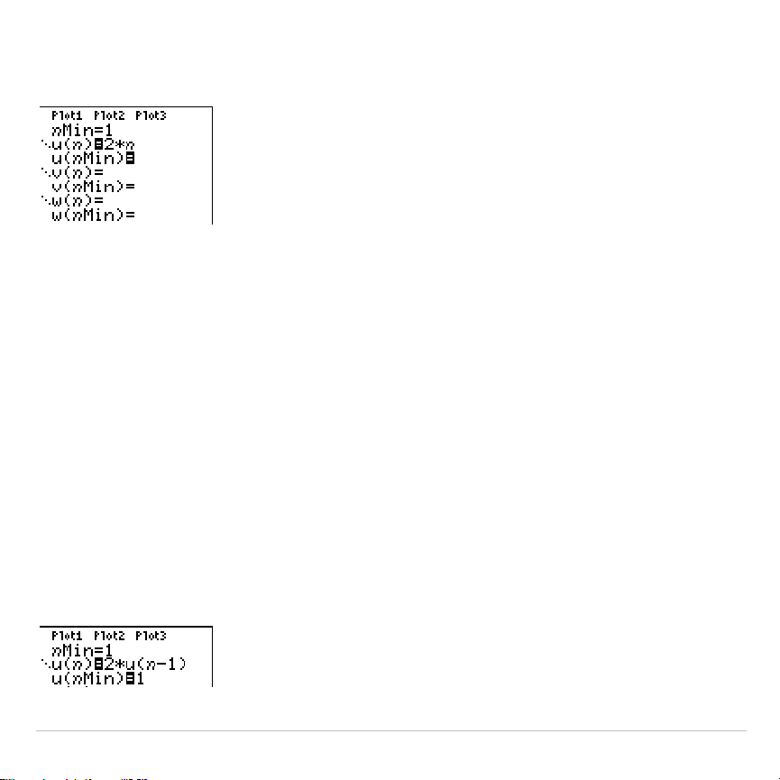
TI-83 Plus Sequence Graphing 183
For example, in the nonrecursive sequence below, you can calculate
u(5)
directly, without first calculating
u(1)
or any previous term.
The sequence equation above returns the sequence
2
,
4
,
6
,
8
,
10
, …for
n
=
1
,
2
,
3
,
4
,
5
,
… .
Note: You may leave blank the initial value
u(nMin)
when calculating
nonrecursive sequences.
Recursive Sequences
In a recursive sequence, the
n
th term in the sequence is defined in
relation to the previous term or the term that precedes the previous term,
represented by
u(
n
N
1)
and
u(
n
N
2)
. A recursive sequence may also be
defined in relation to
n
, as in
u(
n
)=u(
n
N
1)+
n
.
For example, in the sequence below you cannot calculate
u(5)
without
first calculating
u(1)
,
u(2)
,
u(3)
, and
u(4)
.
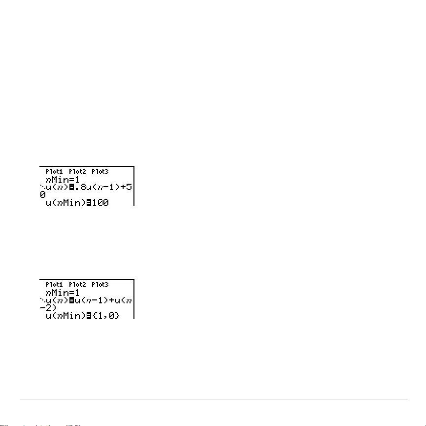
TI-83 Plus Sequence Graphing 184
Using an initial value
u(
n
Min) = 1
, the sequence above returns
1
,
2
,
4
,
8
,
16
, . . .
Tip: On the TI-83 Plus, you must type each character of the terms. For
example, to enter
u(
n
N
1)
, press
y
[
u
]
£
„
¹
À
¤
.
Recursive sequences require an initial value or values, since they
reference undefined terms.
•
If each term in the sequence is defined in relation to the previous
term, as in
u(
n
N
1)
, you must specify an initial value for the first term.
•
If each term in the sequence is defined in relation to the term that
precedes the previous term, as in
u(
n
N
2)
, you must specify initial
values for the first two terms. Enter the initial values as a list enclosed
in braces ({ }) with commas separating the values.
The value of the first term is 0 and the value of the second term is 1 for
the sequence
u(
n
)
.

TI-83 Plus Sequence Graphing 185
Setting Window Variables
To display the window variables, press
p
. These variables define
the viewing window. The values below are defaults for
Seq
graphing in
both
Radian
and
Degree
angle modes.
nMin=1
Smallest
n
value to evaluate
nMax
=
10
Largest
n
value to evaluate
PlotStart
=
1
First term number to be plotted
PlotStep
=
1
Incremental
n
value (for graphing only)
Xmin
=
L
10
Smallest
X
value to be displayed
Xmax
=
10
Largest
X
value to be displayed
Xscl
=
1
Spacing between the
X
tick marks
Ymin
=
L
10
Smallest
Y
value to be displayed
Ymax
=
10
Largest
Y
value to be displayed
Yscl
=
1
Spacing between the
Y
tick marks
n
Min
must be an integer
‚
0.
n
Max
,
PlotStart
, and
PlotStep
must be
integers
‚
1.
n
Min
is the smallest
n
value to evaluate.
n
Min
also is displayed in the
sequence
Y=
editor.
n
Max
is the largest
n
value to evaluate. Sequences
are evaluated at
u(
n
Min)
,
u(
n
Min+1)
,
u(
n
Min+2)
, . . . ,
u(
n
Max)
.

TI-83 Plus Sequence Graphing 186
PlotStart
is the first term to be plotted.
PlotStart=1
begins plotting on the
first term in the sequence. If you want plotting to begin with the fifth term
in a sequence, for example, set
PlotStart=5
. The first four terms are
evaluated but are not plotted on the graph.
PlotStep
is the incremental
n
value for graphing only.
PlotStep
does not
affect sequence evaluation; it only designates which points are plotted
on the graph. If you specify
PlotStep=2
, the sequence is evaluated at
each consecutive integer, but it is plotted on the graph only at every
other integer.

TI-83 Plus Sequence Graphing 187
Selecting Axes Combinations
Setting the Graph Format
To display the current graph format settings, press
y
.
. Chapter
3 describes the format settings in detail. The other graphing modes
share these format settings. The axes setting on the top line of the
screen is available only in
Seq
mode.
Time Web uv vw uw
Type of sequence plot (axes)
RectGC PolarGC
Rectangular or polar output
CoordOn CoordOff
Cursor coordinate display on/off
GridOff GridOn
Grid display off or on
AxesOn AxesOff
Axes display on or off
LabelOff LabelOn
Axes label display off or on
ExprOn ExprOff
Expression display on or off
Setting Axes Format
For sequence graphing, you can select from five axes formats. The table
below shows the values that are plotted on the x-axis and y-axis for each
axes setting.
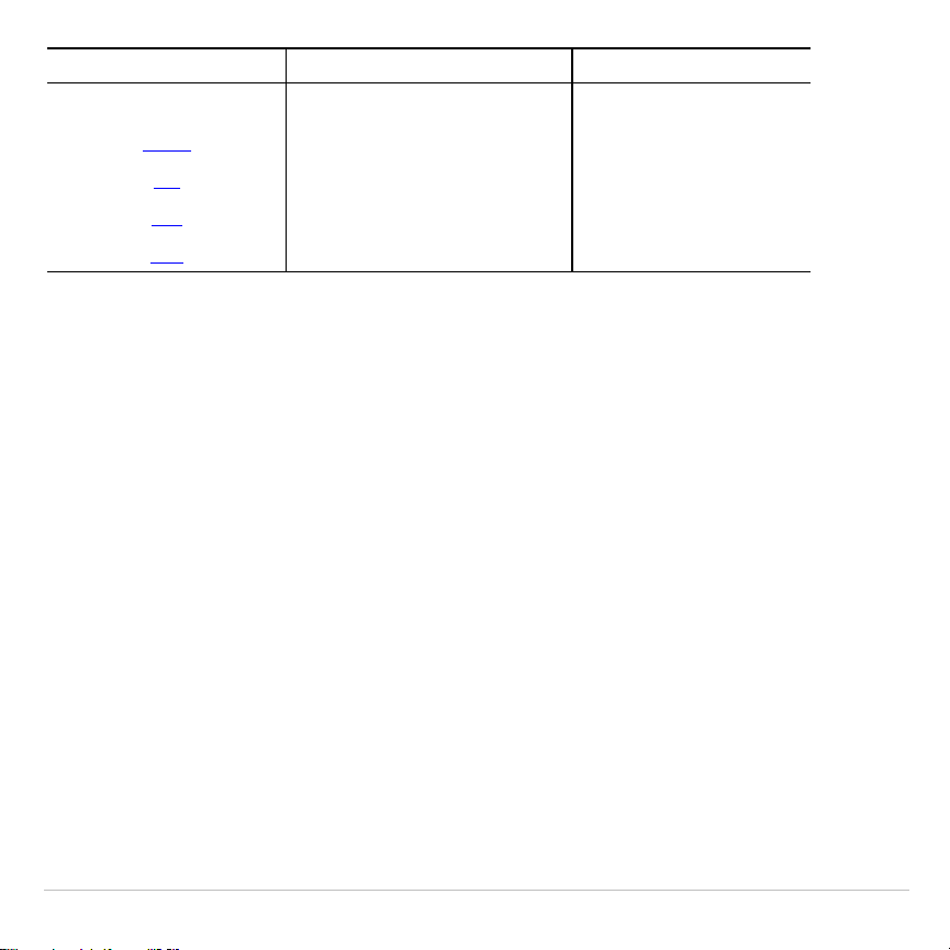
TI-83 Plus Sequence Graphing 188
Axes Setting x-axis y-axis
Time
n
u(
n
)
,
v(
n
)
,
w(
n
)
Web u(
n
N
1)
,
v(
n
N
1)
,
w(
n
N
1) u(
n
)
,
v(
n
)
,
w(
n
)
uv u(
n
)v(
n
)
vw v(
n
)w(
n
)
uw u(
n
)w(
n
)
Displaying a Sequence Graph
To plot the selected sequence functions, press
s
. As a graph is
plotted, the TI-83 Plus updates
X
,
Y
, and
n
.
Smart Graph applies to sequence graphs (Chapter 3).

TI-83 Plus Sequence Graphing 189
Exploring Sequence Graphs
Free-Moving Cursor
The free-moving cursor in
Seq
graphing works the same as in
Func
graphing. In
RectGC
format, moving the cursor updates the values of
X
and
Y
; if
CoordOn
format is selected,
X
and
Y
are displayed. In
PolarGC
format,
X
,
Y
,
R
, and
q
are updated; if
CoordOn
format is selected,
R
and
q
are displayed.
TRACE
The axes format setting affects
TRACE
.
When
Time
,
uv
,
vw
, or
uw
axes format is selected,
TRACE
moves the
cursor along the sequence one
PlotStep
increment at a time. To move
five plotted points at once, press
y
~
or
y
|
.
•
When you begin a trace, the trace cursor is on the first selected
sequence at the term number specified by
PlotStart
, even if it is
outside the viewing window.
•
Quick Zoom applies to all directions. To center the viewing window
on the current cursor location after you have moved the trace cursor,
press
Í
. The trace cursor returns to
n
Min
.
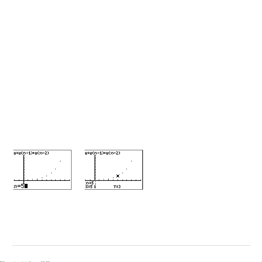
TI-83 Plus Sequence Graphing 190
In
Web
format, the trail of the cursor helps identify points with attracting
and repelling behavior in the sequence. When you begin a trace, the
cursor is on the x-axis at the initial value of the first selected function.
Tip: To move the cursor to a specified
n
during a trace, enter a value for
n
, and
press
Í
. For example, to quickly return the cursor to the beginning of the
sequence, paste
nMin
to the
n=
prompt and press
Í
.
Moving the Trace Cursor to Any Valid
n
Value
To move the trace cursor to any valid
n
value on the current function,
enter the number. When you enter the first digit, an
n
=
prompt and the
number you entered are displayed in the bottom-left corner of the
screen. You can enter an expression at the
n
=
prompt. The value must
be valid for the current viewing window. When you have completed the
entry, press
Í
to move the cursor.

TI-83 Plus Sequence Graphing 191
ZOOM
ZOOM
operations in
Seq
graphing work the same as in
Func
graphing.
Only the
X
(
Xmin
,
Xmax
, and
Xscl
) and
Y
(
Ymin
,
Ymax
, and
Yscl
) window
variables are affected.
PlotStart
,
PlotStep
,
n
Min
, and
n
Max
are only affected when you select
ZStandard
. The
VARS Zoom
secondary menu
ZU
items
1
through
7
are the
ZOOM MEMORY
variables for
Seq
graphing.
CALC
The only
CALC
operation available in
Seq
graphing is
value
.
•
When
Time
axes format is selected,
value
displays
Y
(the
u(
n
)
value)
for a specified
n
value.
•
When
Web
axes format is selected,
value
draws the web and displays
Y
(the
u(
n
)
value) for a specified
n
value.
•
When
uv
,
vw
, or
uw
axes format is selected,
value
displays
X
and
Y
according to the axes format setting. For example, for
uv
axes format,
X
represents
u(
n
)
and
Y
represents
v(
n
)
.
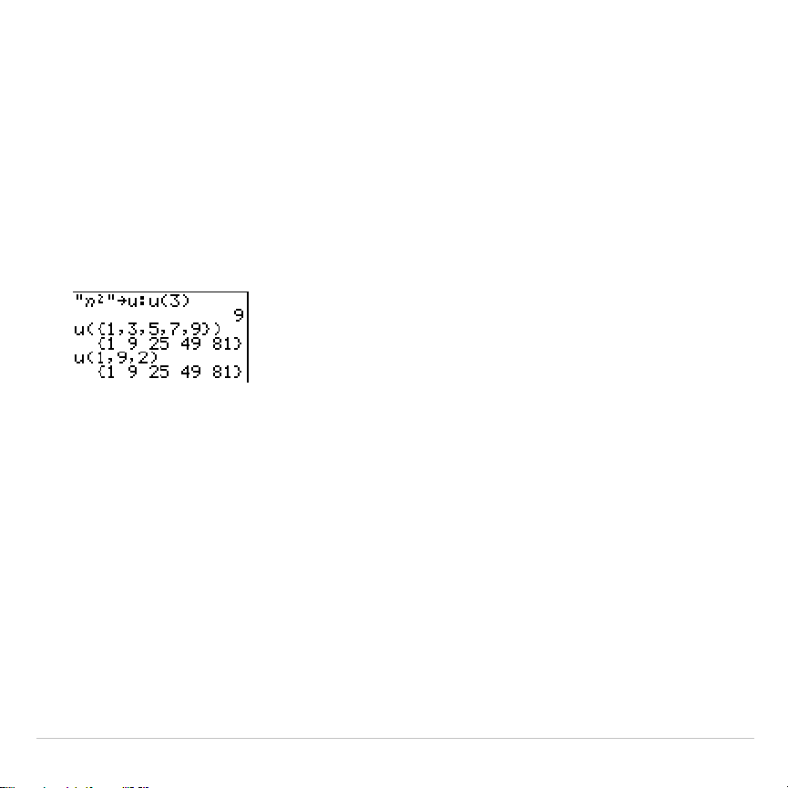
TI-83 Plus Sequence Graphing 192
Evaluating u, v, and w
To enter the sequence names
u
,
v,
or
w
, press
y
[
u
], [
v
], or [
w
]. You can
evaluate these names in any of three ways.
•
Calculate the nth value in a sequence.
•
Calculate a list of values in a sequence.
•
Generate a sequence with
u(
nstart
,
nstop
[,
nstep
])
.
nstep
is optional;
default is 1.

TI-83 Plus Sequence Graphing 193
Graphing Web Plots
Graphing a Web Plot
To select
Web
axes format, press
y
.
~
Í
. A web plot
graphs
u(
n
)
versus
u(
n
N
1)
, which you can use to study long-term
behavior (convergence, divergence, or oscillation) of a recursive
sequence. You can see how the sequence may change behavior as its
initial value changes.
Valid Functions for Web Plots
When
Web
axes format is selected, a sequence will not graph properly or
will generate an error.
•
It must be recursive with only one recursion level (
u(
n
N
1)
but not
u(
n
N
2)
).
•
It cannot reference
n
directly.
•
It cannot reference any defined sequence except itself.

TI-83 Plus Sequence Graphing 194
Displaying the Graph Screen
In
Web
format, press
s
to display the graph screen. The TI-83 Plus:
•
Draws a
y=x
reference line in
AxesOn
format.
•
Plots the selected sequences with
u(
n
N
1)
as the independent
variable.
Note: A potential convergence point occurs whenever a sequence intersects
the y=x reference line. However, the sequence may or may not actually
converge at that point, depending on the sequence’s initial value.
Drawing the Web
To activate the trace cursor, press
r
. The screen displays the
sequence and the current
n
,
X
, and
Y
values (
X
represents
u(
n
N
1)
and
Y
represents
u(
n
)
). Press
~
repeatedly to draw the web step by step,
starting at
n
Min
. In
Web
format, the trace cursor follows this course.
1. It starts on the x-axis at the initial value
u(
n
Min)
(when
PlotStart=1
).
2. It moves vertically (up or down) to the sequence.
3. It moves horizontally to the
y=x
reference line.
4. It repeats this vertical and horizontal movement as you continue to
press
~
.
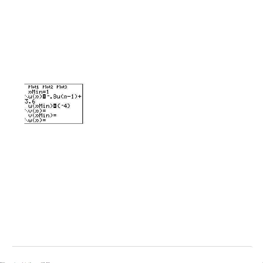
TI-83 Plus Sequence Graphing 195
Using Web Plots to Illustrate Convergence
Example: Convergence
1. Press
o
in
Seq
mode to display the sequence
Y=
editor. Make sure
the graph style is set to
í
(dot), and then define
n
Min
,
u(
n
)
and
u(
n
Min)
as shown below.
2. Press
y
.
Í
to set
Time
axes format.
3. Press
p
and set the variables as shown below.
n
Min=1 Xmin=0 Ymin=
L
10
n
Max=25 Xmax=25 Ymax=10
PlotStart=1 Xscl=1 Yscl=1
PlotStep=1
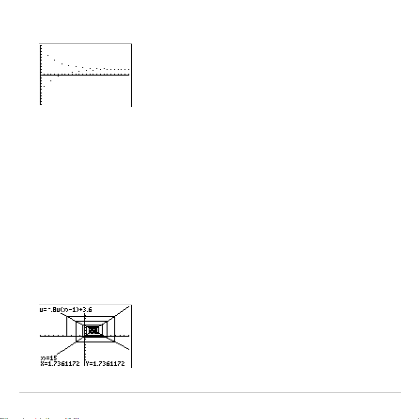
TI-83 Plus Sequence Graphing 196
4. Press
s
to graph the sequence.
5. Press
y
.
and select the
Web
axes setting.
6. Press
p
and change the variables below.
Xmin=
L
10 Xmax=10
7. Press
s
to graph the sequence.
8. Press
r
, and then press
~
to draw the web. The displayed cursor
coordinates
n
,
X
(
u(
n
N
1)
), and
Y
(
u(
n
)
) change accordingly. When you press
~
, a new
n
value is
displayed, and the trace cursor is on the sequence. When you press
~
again, the
n
value remains the same, and the cursor moves to the
y=x
reference line. This pattern repeats as you trace the web.
TI-83 Plus Sequence Graphing 197
Graphing Phase Plots
Graphing with uv, vw, and uw
The phase-plot axes settings
uv
,
vw
, and
uw
show relationships between
two sequences. To select a phase-plot axes setting, press
y
.
,
press
~
until the cursor is on
uv
,
vw
, or
uw
, and then press
Í
.
Axes Setting x-axis y-axis
uv u(
n
)v(
n
)
vw v(
n
)w(
n
)
uw u(
n
)w(
n
)
Example: Predator-Prey Model
Use the predator-prey model to determine the regional populations of a
predator and its prey that would maintain population equilibrium for the
two species.
This example uses the model to determine the equilibrium populations of
foxes and rabbits, with initial populations of 200 rabbits (
u(
n
Min)
) and 50
foxes (
v(
n
Min)
).
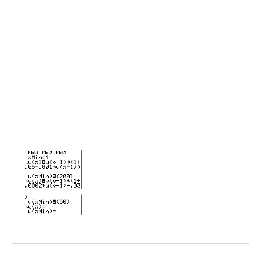
TI-83 Plus Sequence Graphing 198
These are the variables (given values are in parentheses):
R = number of rabbits
M = rabbit population growth rate without foxes (.05)
K = rabbit population death rate with foxes (.001)
W = number of foxes
G = fox population growth rate with rabbits (.0002)
D = fox population death rate without rabbits (.03)
n
= time (in months)
R
n
=R
n
N
1
(1+M
N
KW
n
N
1
)
W
n
=W
n
N
1
(1+GR
n
N
1
N
D)
1. Press
o
in
Seq
mode to display the sequence
Y=
editor. Define the
sequences and initial values for R
n
and W
n
as shown below. Enter
the sequence R
n
as
u(
n
)
and enter the sequence W
n
as
v(
n
)
.
2. Press
y
.
Í
to select
Time
axes format.
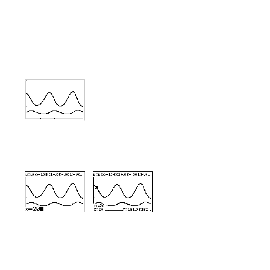
TI-83 Plus Sequence Graphing 199
3. Press
p
and set the variables as shown below.
n
Min=0 Xmin=0 Ymin=0
n
Max=400 Xmax=400 Ymax=300
PlotStart=1 Xscl=100 Yscl=100
PlotStep=1
4. Press
s
to graph the sequence.
5. Press
r
~
to individually trace the number of rabbits (
u(
n
)
) and
foxes (
v(
n
)
) over time (
n
).
Tip: Press a number, and then press
Í
to jump to a specific
n
value
(month) while in
TRACE
.
6. Press
y
.
~
~
Í
to select
uv
axes format.

TI-83 Plus Sequence Graphing 200
7. Press
p
and change these variables as shown below.
Xmin=84 Ymin=25
Xmax=237 Ymax=75
Xscl=50 Yscl=10
8. Press
r
. Trace both the number of rabbits (
X
) and the number of
foxes (
Y
) through 400 generations.
Note: When you press
r
, the equation
for
u
is displayed in the top-left corner. Press
}
or
†
to see the equation for
v
.

TI-83 Plus Sequence Graphing 201
Comparing TI-83 Plus and TI-82 Sequence
Variables
Sequences and Window Variables
Refer to the table if you are familiar with the TI
-
82. It shows TI-83 Plus
sequences and sequence window variables, as well as their TI
-
82
counterparts.
TI-83 Plus TI
.
82
In the
Y=
editor:
u(
n
)U
n
u(
n
Min) U
n
Start
(window variable)
v(
n
)V
n
v(
n
Min) V
n
Start
(window variable)
w(
n
)
not available
w(
n
Min)
not available
In the window editor:
n
Min
n
Start
n
Max
n
Max
PlotStart
n
Min
PlotStep
not available

TI-83 Plus Sequence Graphing 202
Keystroke Differences Between TI-83 Plus
and TI-82
Sequence Keystroke Changes
Refer to the table if you are familiar with the TI
-
82. It compares
TI-83 Plus sequence-name syntax and variable syntax with TI
.
82
sequence-name syntax and variable syntax.
TI-83 Plus / TI-82 On TI-83 Plus, press: On TI-82, press:
n
/
n
„y
[
n
]
u(
n
)
/
U
n
y
[
u
]
£
„
¤
y
ó
¶
À
v(
n
) / V
n
y
[
v
]
£
„
¤
y
ó
¶
Á
w(
n
)
y
[
w
]
£
„
¤
not available
u(
n
N
1) / U
n
N
1
y
[
u
]
£
„
¹
À
¤
y
õ
v(
n
N
1) / V
n
N
1
y
[
v
]
£
„
¹
À
¤
y
ö
w(
n
N
1)
y
[
w
]
£
„
¹
À
¤
not available
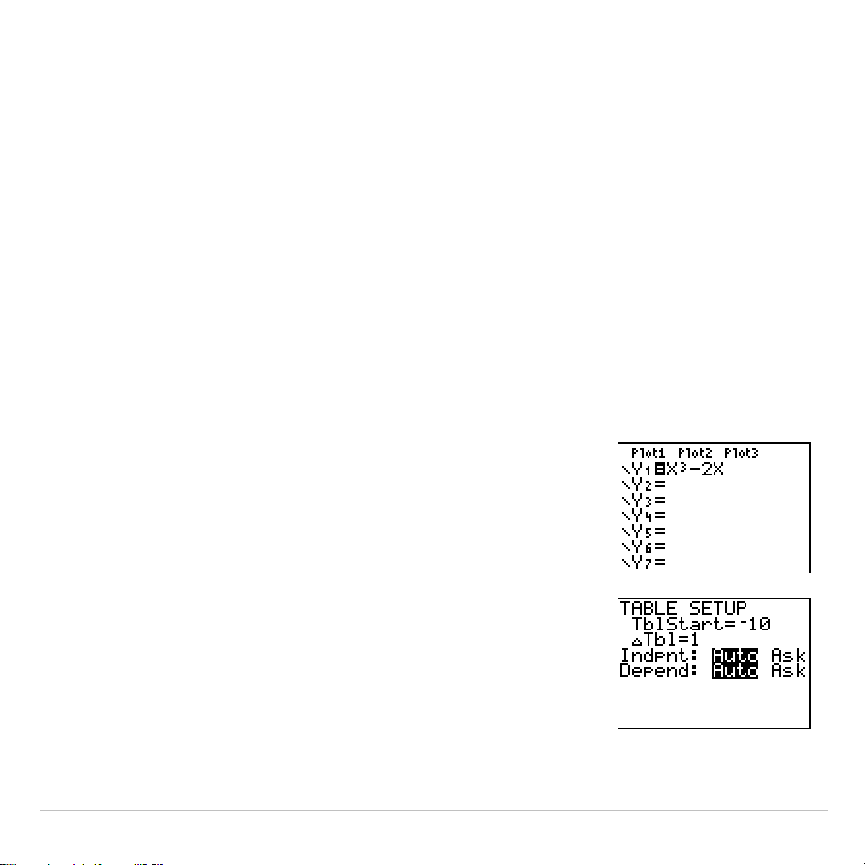
TI-83 Plus Tables 203
Chapter 7:
Tables
Getting Started: Roots of a Function
Getting Started is a fast-paced introduction. Read the chapter for details.
Evaluate the function Y = X
3
N
2X at each integer between
L
10 and 10. How many
sign changes occur, and at what X values?
1. Press
z
†
†
†
Í
to set
Func
graphing
mode.
2. Press
o
. Press
„
3
to select
3
.
Then press
¹
2
„
to enter the function
Y
1
=X
3
N
2X
.
3. Press
y
-
to display the
TABLE SETUP
screen. Press
Ì
10
Í
to set
TblStart=
L
10
.
Press
1
Í
to set
@
Tbl=1
.
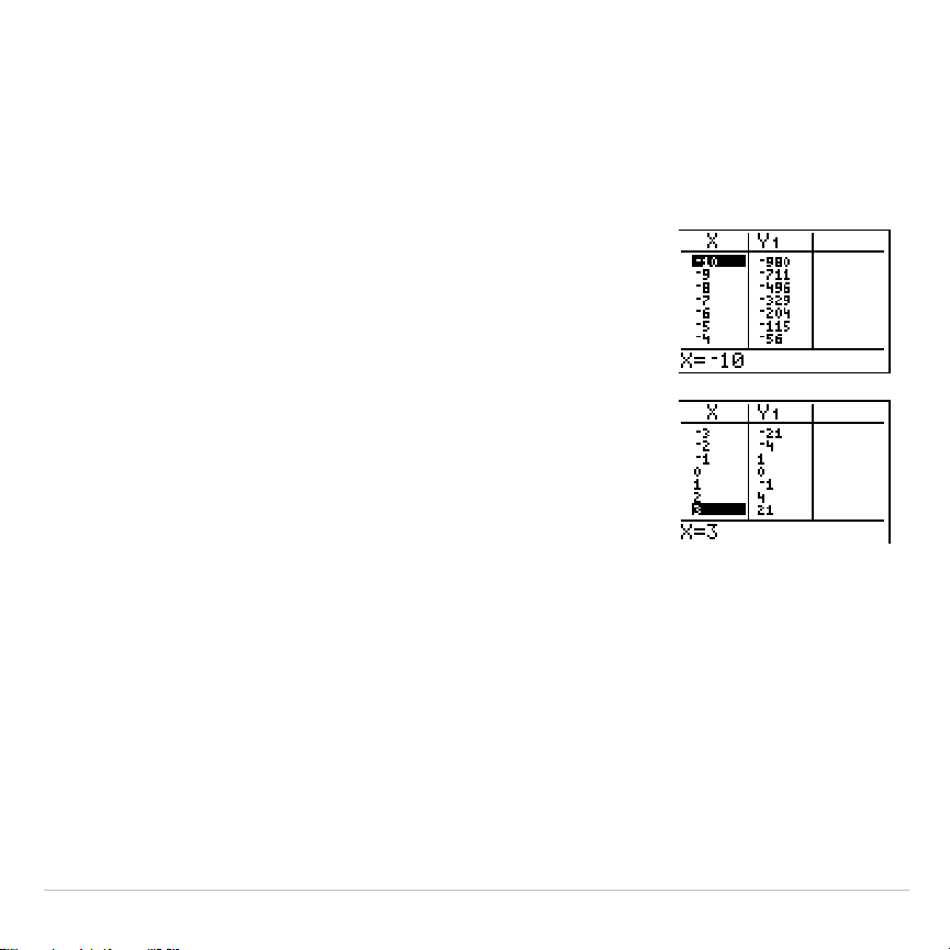
TI-83 Plus Tables 204
Press
Í
to select
Indpnt: Auto
(automatically generated independent values).
Press
†
Í
to select
Depend: Auto
(automatically generated dependent values).
4. Press
y
0
to display the table screen.
5. Press
†
until you see the sign changes in the
value of
Y
1
. How many sign changes occur, and
at what
X
values?
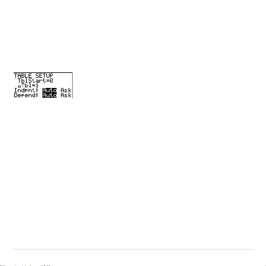
TI-83 Plus Tables 205
Setting Up the Table
TABLE SETUP Screen
To display the
TABLE SETUP
screen, press
y
-
.
TblStart,
@
Tbl
TblStart
(table start) defines the initial value for the independent variable.
TblStart
applies only when the independent variable is generated
automatically (when
Indpnt: Auto
is selected).
@
Tbl
(table step) defines the increment for the independent variable.
Note: In
Seq
mode, both
TblStart
and
@
Tbl
must be integers.

TI-83 Plus Tables 206
Indpnt: Auto, Indpnt: Ask, Depend: Auto, Depend: Ask
Selections Table Characteristics
Indpnt: Auto
Depend: Auto
Values are displayed automatically in both the
independent-variable column and in all dependent-
variable columns.
Indpnt: Ask
Depend: Auto
The table is empty; when you enter a value for the
independent variable, all corresponding dependent-
variable values are calculated and displayed
automatically.
Indpnt: Auto
Depend: Ask
Values are displayed automatically for the independent
variable; to generate a value for a dependent variable,
move the cursor to that cell and press
Í
.
Indpnt: Ask
Depend: Ask
The table is empty; enter values for the independent
variable; to generate a value for a dependent variable,
move the cursor to that cell and press
Í
.
Setting Up the Table from the Home Screen or a Program
To store a value to
TblStart
,
@
Tbl
, or
Tbl
Z
nput
from the home screen or a
program, select the variable name from the
VARS TABLE
secondary menu.
Tbl
Z
nput
is a list of independent-variable values in the current table.
When you press
y
-
in the program editor, you can select
IndpntAuto
,
IndpntAsk
,
DependAuto
, and
DependAsk
.
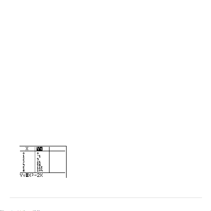
TI-83 Plus Tables 207
Defining the Dependent Variables
Defining Dependent Variables from the Y= Editor
In the
Y=
editor, enter the functions that define the dependent variables.
Only functions that are selected in the
Y=
editor are displayed in the
table. The current graphing mode is used. In
Par
mode, you must define
both components of each parametric equation (Chapter 4).
Editing Dependent Variables from the Table Editor
To edit a selected
Y=
function from the table editor, follow these steps.
1. Press
y
0
to display the table, then press
~
or
|
to move the
cursor to a dependent-variable column.
2. Press
}
until the cursor is on the function name at the top of the
column. The function is displayed on the bottom line.
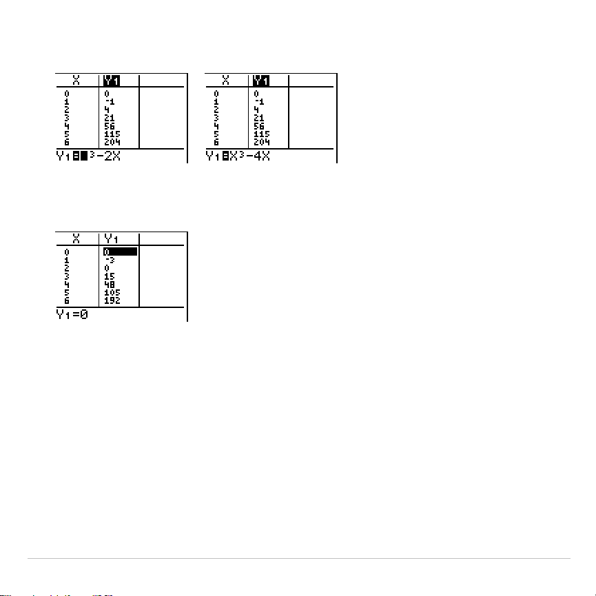
TI-83 Plus Tables 208
3. Press
Í
. The cursor moves to the bottom line. Edit the function.
4. Press
Í
or
†
. The new values are calculated. The table and the
Y=
function are updated automatically.
Note:
You also can use this feature to view the function that defines a
dependent variable without having to leave the table.
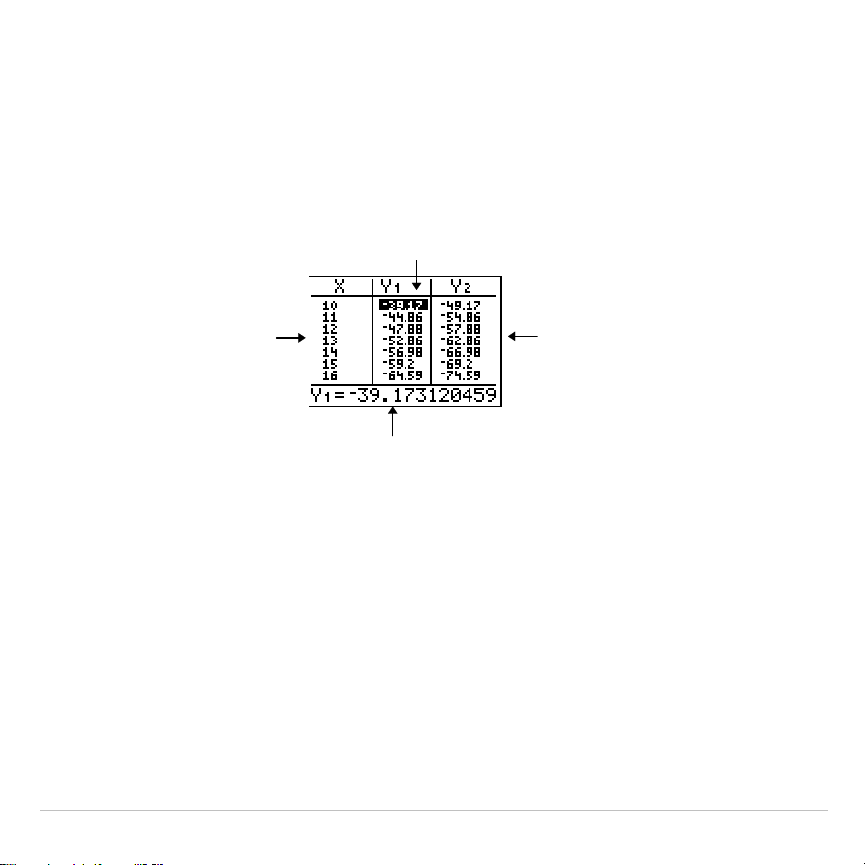
TI-83 Plus Tables 209
Displaying the Table
The Table
To display the table, press
y
0
.
Current cell
Independent-variable
values in the first column
Dependent-variable
values in the second
and third columns
Current cell’s full value
Note: The table abbreviates the values, if necessary.
Independent and Dependent Variables
The current graphing mode determines which independent and
dependent variables are displayed in the table (Chapter 1). In the table
above, for example, the independent variable
X
and the dependent
variables
Y
1
and
Y
2
are displayed because
Func
graphing mode is set.

TI-83 Plus Tables 210
Graphing Mode Independent Variable Dependent Variable
Func
(function)
XY
1
through
Y
9
, and
Y
0
Par
(parametric)
TX
1T
/
Y
1T
through
X
6T
/
Y
6T
Pol
(polar)
q
r
1
through
r
6
Seq
(sequence)
n
u(
n
)
,
v(
n
)
, and
w(
n
)
Clearing the Table from the Home Screen or a Program
From the home screen, select the
ClrTable
instruction from the
CATALOG
.
To clear the table, press
Í
.
From a program, select
9:ClrTable
from the
PRGM I/O
menu or from the
CATALOG
. The table is cleared upon execution. If
IndpntAsk
is selected,
all independent and dependent variable values on the table are cleared.
If
DependAsk
is selected, all dependent variable values on the table are
cleared.
Scrolling Independent-Variable Values
If
Indpnt: Auto
is selected, you can press
}
and
†
in the independent-
variable column to display more values. As you scroll the column, the
corresponding dependent-variable values also are displayed. All
dependent-variable values may not be displayed if
Depend: Ask
is
selected.
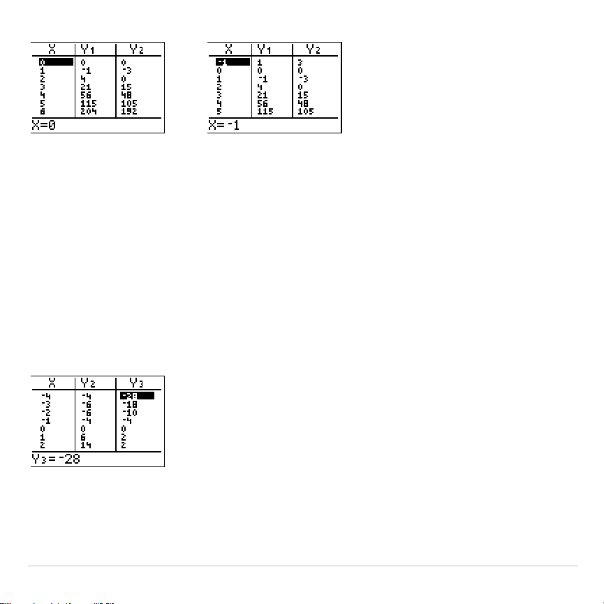
TI-83 Plus Tables 211
Note:
You can scroll back from the value entered for
TblStart
. As you scroll,
TblStart
is updated automatically to the value shown on the top line of the table.
In the example above,
TblStart=0
and
@
Tbl=1
generates and displays values of
X=0
, …,
6
; but you can press
}
to scroll back and display the table for
X=
M
1
, …,
5
.
Displaying Other Dependent Variables
If you have defined more than two dependent variables, the first two
selected
Y=
functions are displayed initially. Press
~
or
|
to display
dependent variables defined by other selected
Y=
functions. The
independent variable always remains in the left column, except during a
trace with
Par
graphing mode and
G
.
T
split-screen mode set.
Tip:
To simultaneously display two dependent variables on the table that are not
defined as consecutive Y= functions, go to the Y= editor and deselect the Y=
functions between the two you want to display. For example, to simultaneously
display
Y
4
and
Y
7
on the table, go to the Y= editor and deselect
Y
5
and
Y
6
.
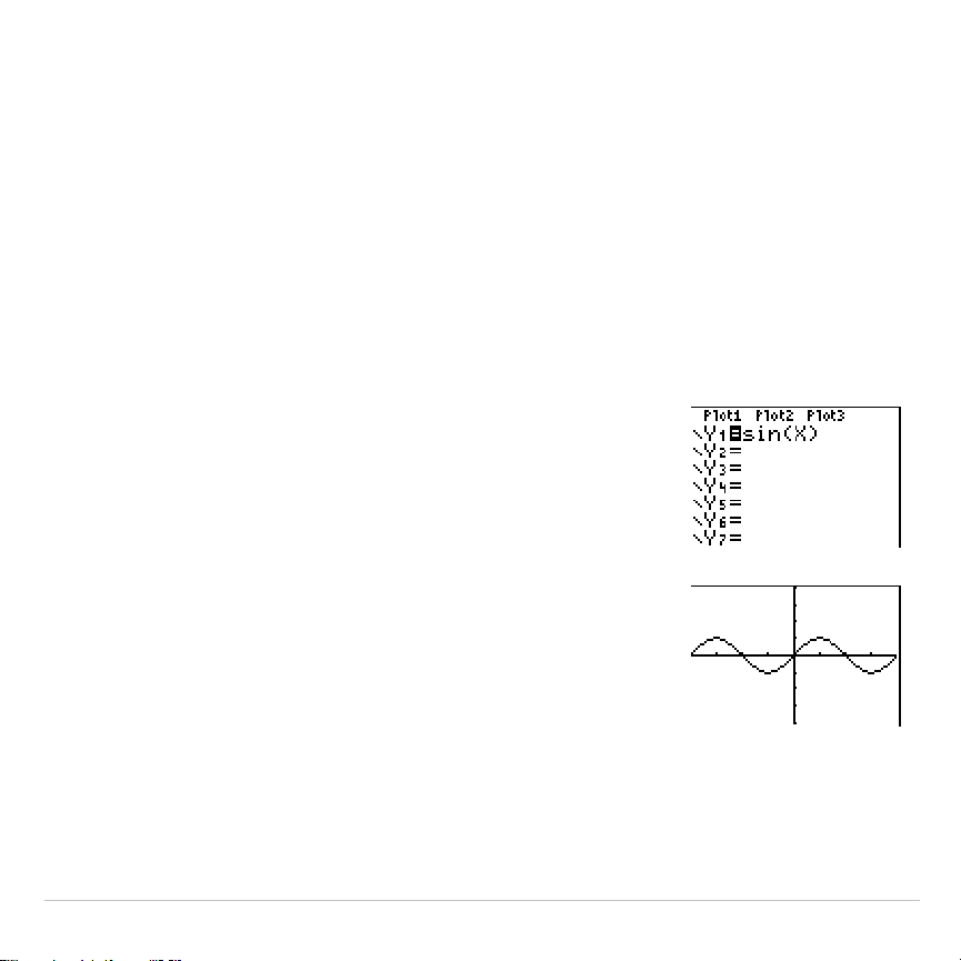
TI-83 Plus Draw Instructions 212
Chapter 8:
Draw Instructions
Getting Started: Drawing a Tangent Line
Getting Started is a fast-paced introduction. Read the chapter for details.
Suppose you want to find the equation of the tangent line at X =
‡
2/2 for the
function Y = sin(X).
Before you begin, select
Radian
and
Func
mode
from the mode screen, if necessary.
1. Press
o
to display the
Y=
editor. Press
˜
„
¤
to store
sin(X)
in
Y
1
.
2. Press
q
7
to select
7:ZTrig
, which graphs
the equation in the Zoom Trig window.
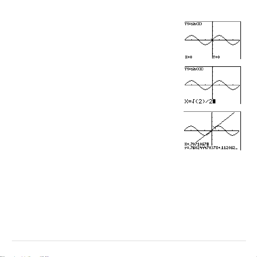
TI-83 Plus Draw Instructions 213
3. Press
y
<
5
to select
5:Tangent(
. The
tangent instruction is initiated.
4. Press
y
C
2
¤
¥
2
.
5. Press
Í
. The tangent line is drawn; the
X
value and the tangent-line equation are
displayed on the graph.

TI-83 Plus Draw Instructions 214
Using the DRAW Menu
DRAW Menu
To display the
DRAW
menu, press
y
<
. The TI-83 Plus’s
interpretation of these instructions depends on whether you accessed
the menu from the home screen or the program editor or directly from a
graph.
DRAW POINTS STO
1:ClrDraw
Clears all drawn elements.
2:Line(
Draws a line segment between 2 points.
3:Horizontal
Draws a horizontal line.
4:Vertical
Draws a vertical line.
5:Tangent(
Draws a line segment tangent to a function.
6:DrawF
Draws a function.
7:Shade(
Shades an area between two functions.
8:DrawInv
Draws the inverse of a function.
9:Circle(
Draws a circle.
0:Text(
Draws text on a graph screen.
A:Pen
Activates the free-form drawing tool.

TI-83 Plus Draw Instructions 215
Before Drawing on a Graph
The
DRAW
instructions draw on top of graphs. Therefore, before you use
the
DRAW
instructions, consider whether you want to perform one or more
of the following actions.
•
Change the mode settings on the mode screen.
•
Change the format settings on the format screen.
•
Enter or edit functions in the
Y=
editor.
•
Select or deselect functions in the
Y=
editor.
•
Change the window variable values.
•
Turn stat plots on or off.
•
Clear existing drawings with
ClrDraw
.
Note: If you draw on a graph and then perform any of the actions listed above,
the graph is replotted without the drawings when you display the graph again.
Drawing on a Graph
You can use any
DRAW
menu instructions except
DrawInv
to draw on
Func
,
Par
,
Pol
, and
Seq
graphs.
DrawInv
is valid only in
Func
graphing.
The coordinates for all
DRAW
instructions are the display’s x-coordinate
and y-coordinate values.
TI-83 Plus Draw Instructions 216
You can use most
DRAW
menu and
DRAW POINTS
menu instructions to
draw directly on a graph, using the cursor to identify the coordinates.
You also can execute these instructions from the home screen or from
within a program. If a graph is not displayed when you select a
DRAW
menu instruction, the home screen is displayed.
TI-83 Plus Draw Instructions 217
Clearing Drawings
Clearing Drawings When a Graph Is Displayed
All points, lines, and shading drawn on a graph with
DRAW
instructions
are temporary.
To clear drawings from the currently displayed graph, select
1:ClrDraw
from the
DRAW
menu. The current graph is replotted and displayed with
no drawn elements.
Clearing Drawings from the Home Screen or a Program
To clear drawings on a graph from the home screen or a program, begin
on a blank line on the home screen or in the program editor. Select
1:ClrDraw
from the
DRAW
menu. The instruction is copied to the cursor
location. Press
Í
.
When
ClrDraw
is executed, it clears all drawings from the current graph
and displays the message
Done
. When you display the graph again, all
drawn points, lines, circles, and shaded areas will be gone.
Note: Before you clear drawings, you can store them with
StorePic
.
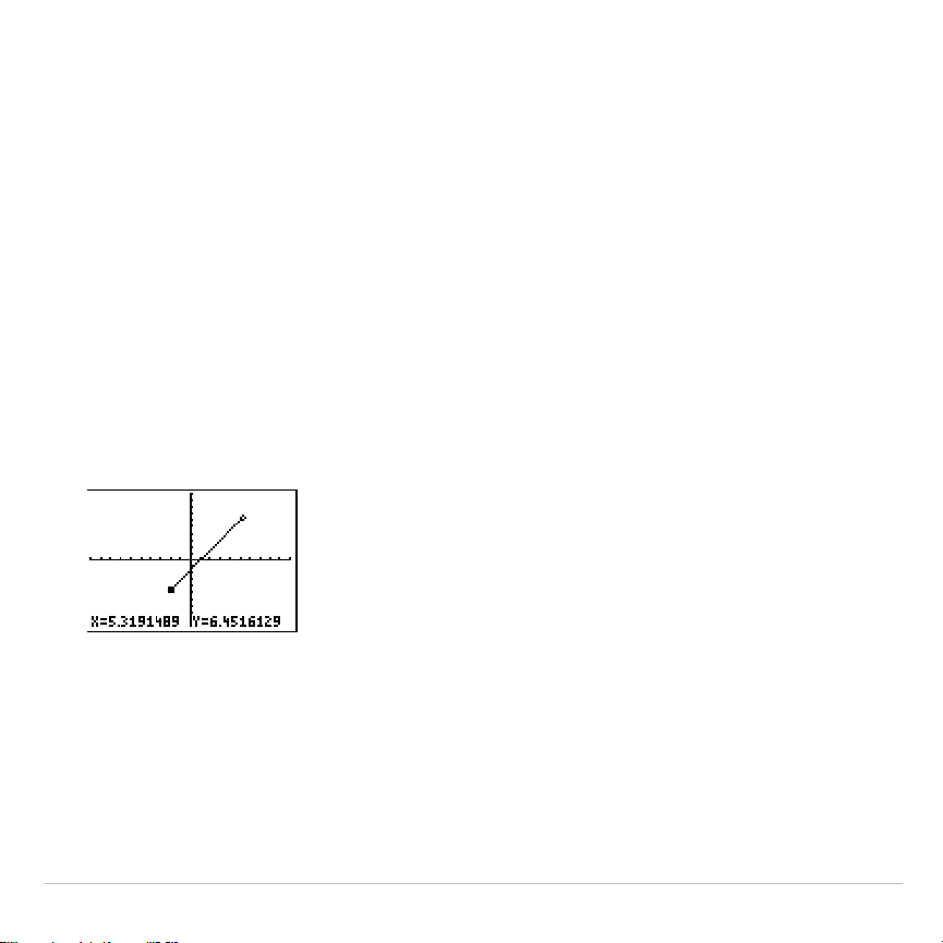
TI-83 Plus Draw Instructions 218
Drawing Line Segments
Drawing a Line Segment Directly on a Graph
To draw a line segment when a graph is displayed, follow these steps.
1. Select
2:Line(
from the
DRAW
menu.
2. Place the cursor on the point where you want the line segment to
begin, and then press
Í
.
3. Move the cursor to the point where you want the line segment to end.
The line is displayed as you move the cursor. Press
Í
.
To continue drawing line segments, repeat steps 2 and 3. To cancel
Line(
, press
‘
.
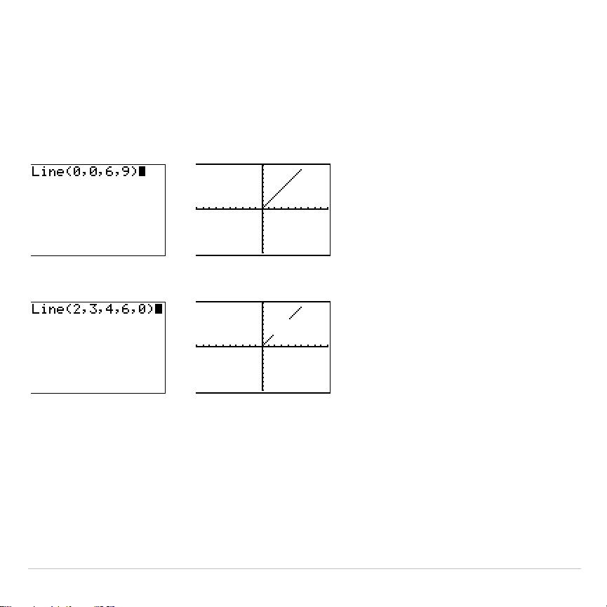
TI-83 Plus Draw Instructions 219
Drawing a Line Segment from the Home Screen or a Program
Line(
also draws a line segment between the coordinates (
X1,Y1
) and
(
X2,Y2
). The values may be entered as expressions.
Line(
X1,Y1,X2,Y2
)
To erase a line segment, enter
Line(
X1,Y1,X2,Y2,
0)

TI-83 Plus Draw Instructions 220
Drawing Horizontal and Vertical Lines
Drawing a Line Directly on a Graph
To draw a horizontal or vertical line when a graph is displayed, follow
these steps.
1. Select
3:Horizontal
or
4:Vertical
from the
DRAW
menu. A line is
displayed that moves as you move the cursor.
2. Place the cursor on the y-coordinate (for horizontal lines) or
x-coordinate (for vertical lines) through which you want the drawn line
to pass.
3. Press
Í
to draw the line on the graph.
To continue drawing lines, repeat steps 2 and 3.
To cancel
Horizontal
or
Vertical
, press
‘
.
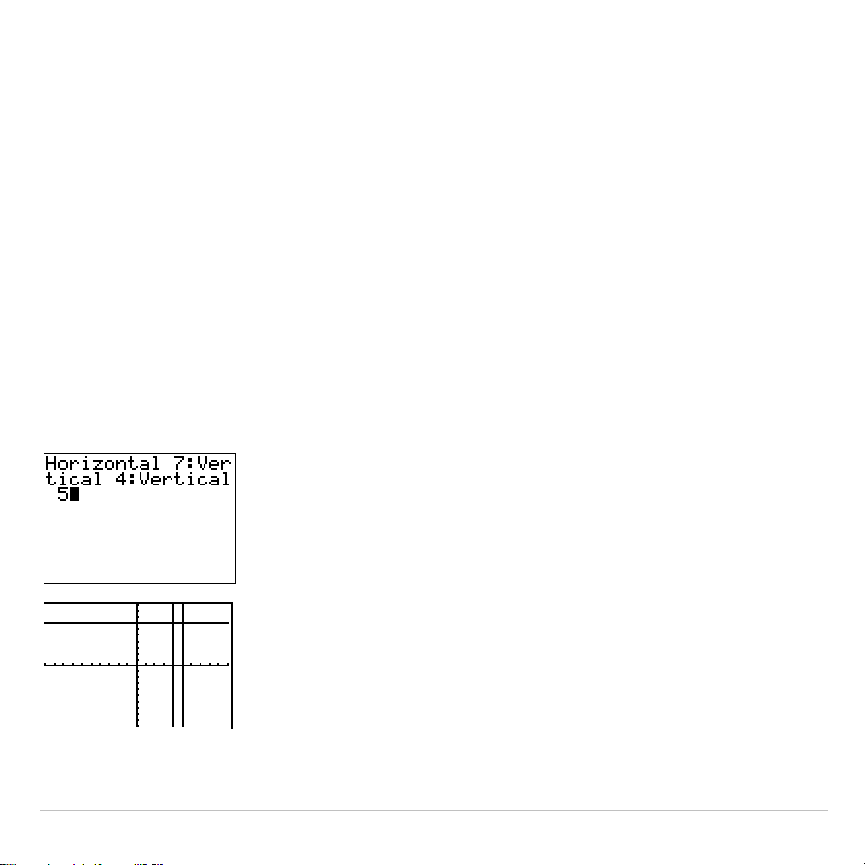
TI-83 Plus Draw Instructions 221
Drawing a Line from the Home Screen or a Program
Horizontal
(horizontal line) draws a horizontal line at
Y=
y
.
y
can be an
expression but not a list.
Horizontal
y
Vertical
(vertical line) draws a vertical line at
X
=
x
.
x
can be an expression
but not a list.
Vertical
x
To instruct the TI-83 Plus to draw more than one horizontal or vertical
line, separate each instruction with a colon (
:
).
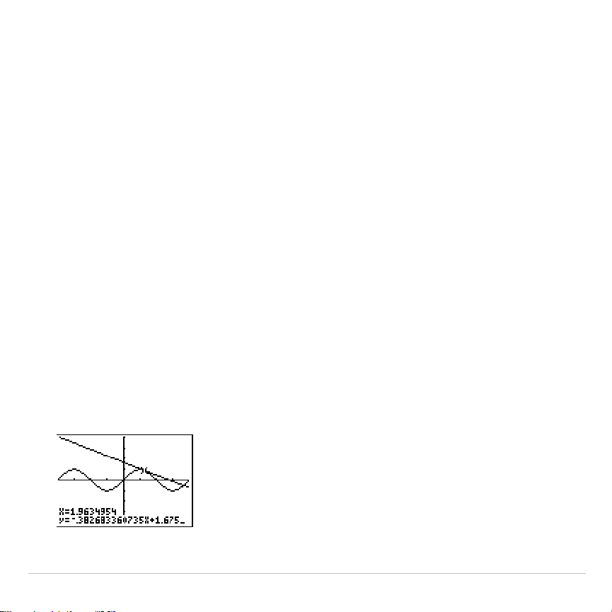
TI-83 Plus Draw Instructions 222
Drawing Tangent Lines
Drawing a Tangent Line Directly on a Graph
To draw a tangent line when a graph is displayed, follow these steps.
1. Select
5:Tangent(
from the
DRAW
menu.
2. Press
†
and
}
to move the cursor to the function for which you want
to draw the tangent line. The current graph’s
Y=
function is displayed
in the top-left corner, if
ExprOn
is selected.
3. Press
~
and
|
or enter a number to select the point on the function at
which you want to draw the tangent line.
4. Press
Í
. In
Func
mode, the
X
value at which the tangent line was
drawn is displayed on the bottom of the screen, along with the
equation of the tangent line. In all other modes, the
dy/dx
value is
displayed.
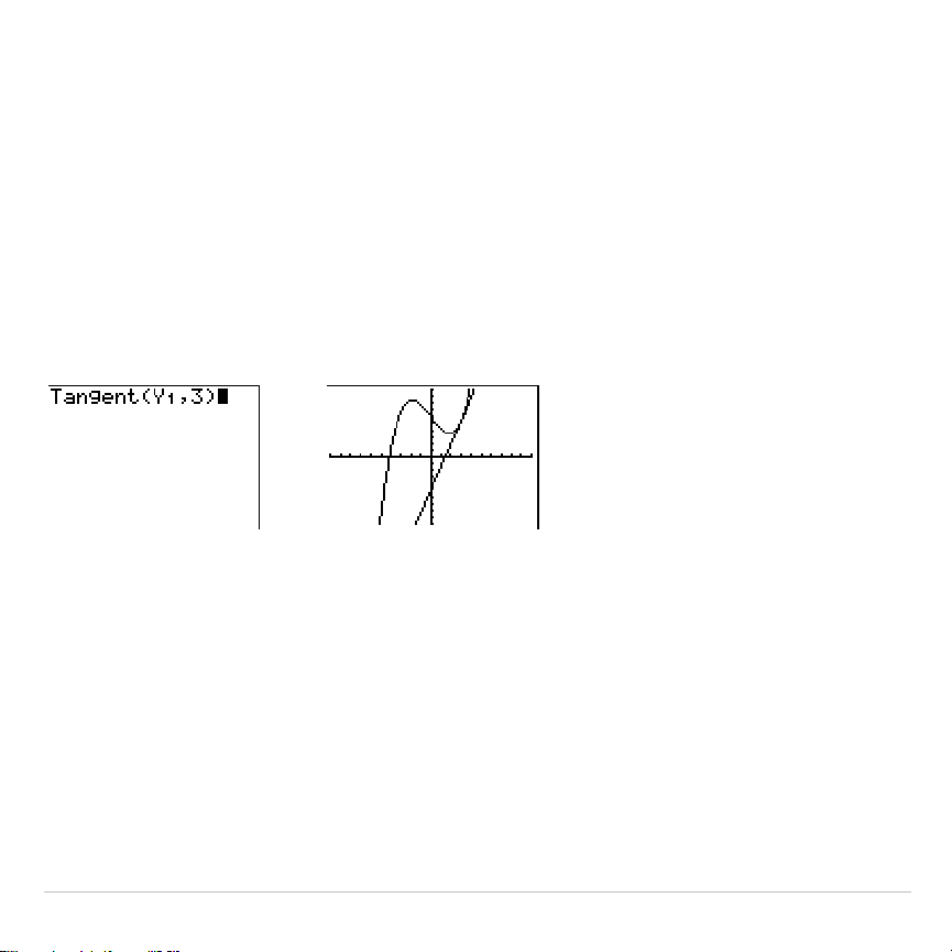
TI-83 Plus Draw Instructions 223
Tip:
Change the fixed decimal setting on the mode screen if you want to see
fewer digits displayed for
X
and the equation for
Y
.
Drawing a Tangent Line from the Home Screen or a Program
Tangent(
(tangent line) draws a line tangent to
expression
in terms of
X
,
such as
Y
1
or
X
2
, at point
X
=
value
.
X
can be an expression.
expression
is
interpreted as being in
Func
mode.
Tangent(
expression
,
value
)
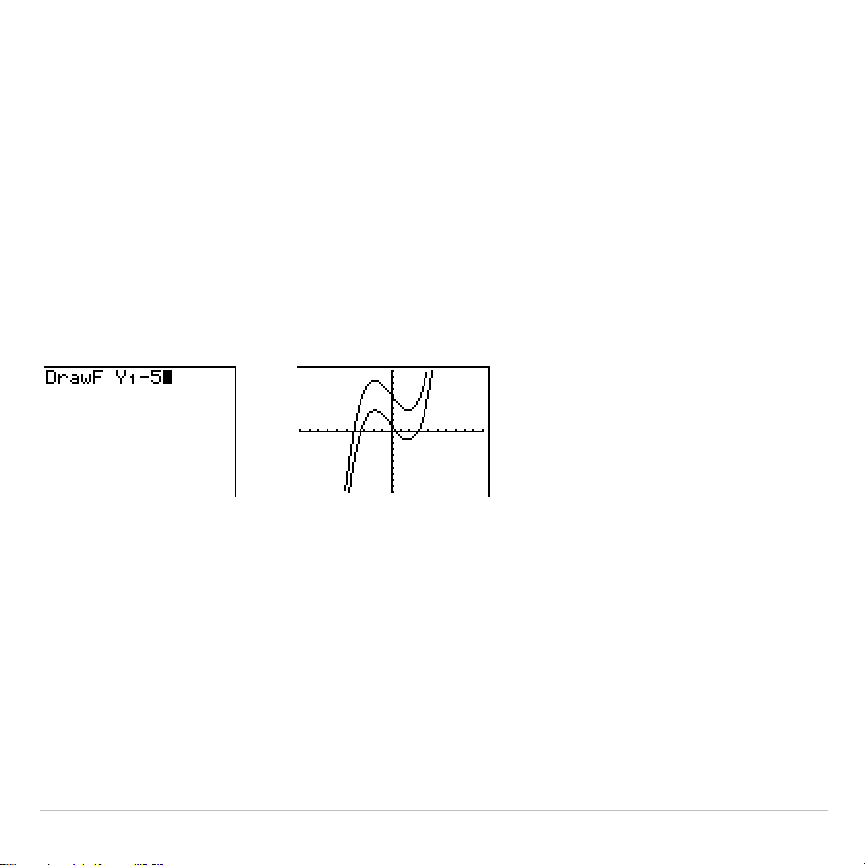
TI-83 Plus Draw Instructions 224
Drawing Functions and Inverses
Drawing a Function
DrawF
(draw function) draws
expression
as a function in terms of
X
on the
current graph. When you select
6:DrawF
from the
DRAW
menu, the
TI-83 Plus returns to the home screen or the program editor.
DrawF
is not
interactive.
DrawF
expression
Note: You cannot use a list in
expression
to draw a family of curves.
Drawing an Inverse of a Function
DrawInv
(draw inverse) draws the inverse of
expression
by plotting
X
values
on the y-axis and
Y
values on the x-axis. When you select
8:DrawInv
from
the
DRAW
menu, the TI-83 Plus returns to the home screen or the
program editor.
DrawInv
is not interactive.
DrawInv
works in
Func
mode
only.
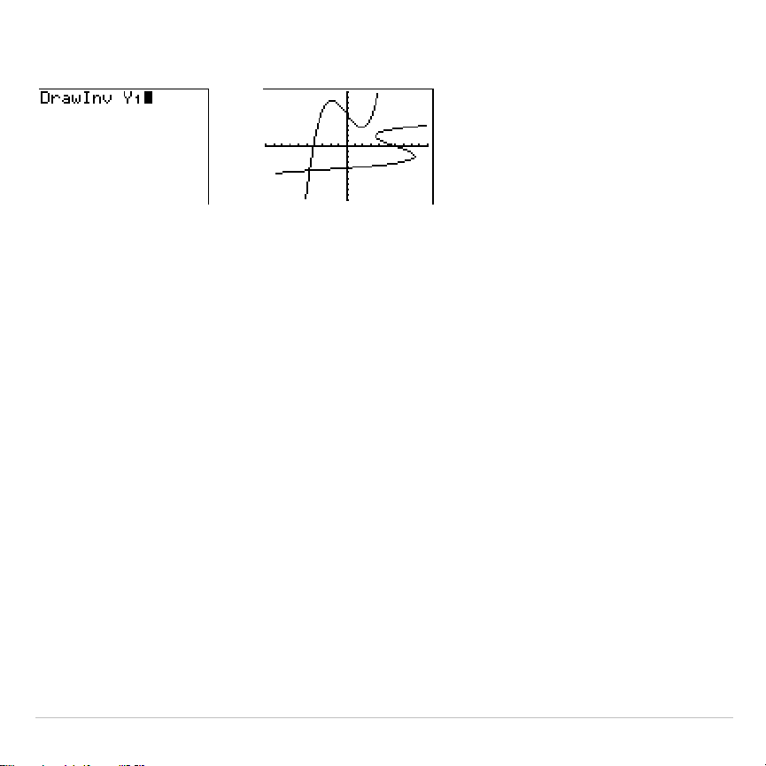
TI-83 Plus Draw Instructions 225
DrawInv
expression
Note: You cannot use a list in
expression
to draw a family of curves.

TI-83 Plus Draw Instructions 226
Shading Areas on a Graph
Shading a Graph
To shade an area on a graph, select
7:Shade(
from the
DRAW
menu. The
instruction is pasted to the home screen or to the program editor.
Shade(
draws
lowerfunc
and
upperfunc
in terms of
X
on the current graph
and shades the area that is specifically above
lowerfunc
and below
upperfunc
. Only the areas where
lowerfunc
<
upperfunc
are shaded.
Xleft
and
Xright
, if included, specify left and right boundaries for the
shading.
Xleft
and
Xright
must be numbers between
Xmin
and
Xmax
,
which are the defaults.
pattern
specifies one of four shading patterns.
pattern
=
1
vertical (default)
pattern
=
2
horizontal
pattern
=
3
negative—slope 45
¡
pattern
=
4
positive—slope 45
¡
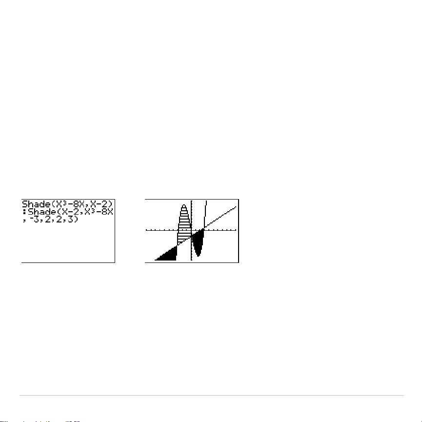
TI-83 Plus Draw Instructions 227
patres
specifies one of eight shading resolutions.
patres
=
1
shades every pixel (default)
patres
=
2
shades every second pixel
patres
=
3
shades every third pixel
patres
=
4
shades every fourth pixel
patres
=
5
shades every fifth pixel
patres
=
6
shades every sixth pixel
patres
=
7
shades every seventh pixel
patres
=
8
shades every eighth pixel
Shade(
lowerfunc,upperfunc[,Xleft,Xright,pattern,patres]
)
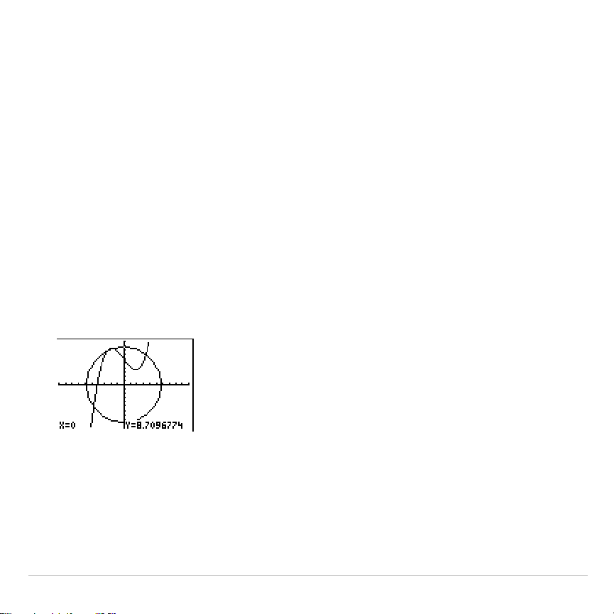
TI-83 Plus Draw Instructions 228
Drawing Circles
Drawing a Circle Directly on a Graph
To draw a circle directly on a displayed graph using the cursor, follow
these steps.
1. Select
9:Circle(
from the
DRAW
menu.
2. Place the cursor at the center of the circle you want to draw. Press
Í
.
3. Move the cursor to a point on the circumference. Press
Í
to draw
the circle on the graph.
Note: This circle is displayed as circular, regardless of the window variable
values, because you drew it directly on the display. When you use the
Circle(
instruction from the home screen or a program, the current window
variables may distort the shape.
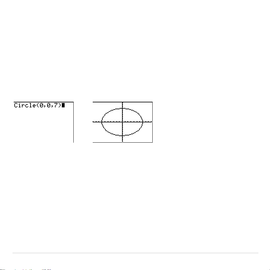
TI-83 Plus Draw Instructions 229
To continue drawing circles, repeat steps 2 and 3. To cancel
Circle(
,
press
‘
.
Drawing a Circle from the Home Screen or a Program
Circle(
draws a circle with center (
X,Y
) and
radius.
These values can be
expressions.
Circle(
X,Y,radius
)
Tip: When you use
Circle(
on the home screen or from a program, the current
window values may distort the drawn circle. Use
ZSquare
(Chapter 3) before
drawing the circle to adjust the window variables and make the circle circular.

TI-83 Plus Draw Instructions 230
Placing Text on a Graph
Placing Text Directly on a Graph
To place text on a graph when the graph is displayed, follow these steps.
1. Select
0:Text(
from the
DRAW
menu.
2. Place the cursor where you want the text to begin.
3. Enter the characters. Press
ƒ
or
y
7
to enter letters and
q
. You may enter TI-83 Plus functions, variables, and instructions.
The font is proportional, so the exact number of characters you can
place on the graph varies. As you type, the characters are placed on
top of the graph.
To cancel
Text(
, press
‘
.
Placing Text on a Graph from the Home Screen or a Program
Text(
places on the current graph the characters comprising
value
, which
can include TI-83 Plus functions and instructions. The top-left corner of
the first character is at pixel (
row,column
), where
row
is an integer between
0 and 57 and
column
is an integer between 0 and 94. Both
row
and
column
can be expressions.
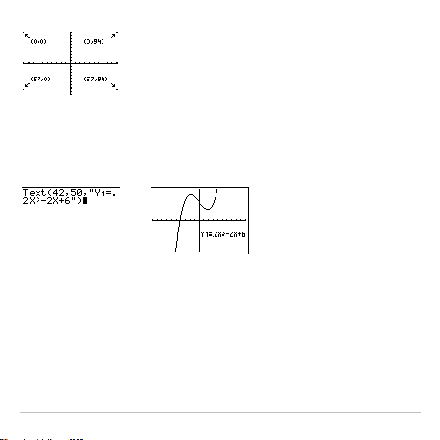
TI-83 Plus Draw Instructions 231
Text(
row,column,value,value…
)
value
can be text enclosed in quotation marks (
"
), or it can be an
expression. The TI-83 Plus will evaluate an expression and display the
result with up to 10 characters.
Split Screen
On a
Horiz
split screen, the maximum value for
row
is 25. On a
G
.
T
split
screen, the maximum value for
row
is 45, and the maximum value for
column
is 46.
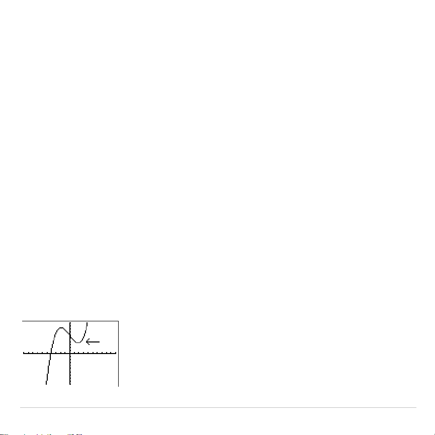
TI-83 Plus Draw Instructions 232
Using Pen to Draw on a Graph
Using Pen to Draw on a Graph
Pen
draws directly on a graph only. You cannot execute
Pen
from the
home screen or a program.
To draw on a displayed graph, follow these steps.
1. Select
A:Pen
from the
DRAW
menu.
2. Place the cursor on the point where you want to begin drawing. Press
Í
to turn on the pen.
3. Move the cursor. As you move the cursor, you draw on the graph,
shading one pixel at a time.
4. Press
Í
to turn off the pen.
For example,
Pen
was used to create the arrow pointing to the local
minimum of the selected function.
Note: To continue drawing on the graph, move the
cursor to a new position where you want to begin
drawing again, and then repeat steps 2, 3, and 4. To
cancel
Pen
, press
‘
.
TI-83 Plus Draw Instructions 233
Drawing Points on a Graph
DRAW POINTS Menu
To display the
DRAW POINTS
menu, press
y
<
~
. The TI-83 Plus’s
interpretation of these instructions depends on whether you accessed
this menu from the home screen or the program editor or directly from a
graph.
DRAW POINTS STO
1:Pt-On(
Turns on a point.
2:Pt-Off(
Turns off a point.
3:Pt-Change(
Toggles a point on or off.
4:Pxl-On(
Turns on a pixel.
5:Pxl-Off(
Turns off a pixel.
6:Pxl-Change(
Toggles a pixel on or off.
7:pxl-Test(
Returns 1 if pixel on, 0 if pixel off.
Drawing Points Directly on a Graph with Pt.On(
To draw a point on a graph, follow these steps.
1. Select
1:Pt
.
On(
from the
DRAW POINTS
menu.
2. Move the cursor to the position where you want to draw the point.
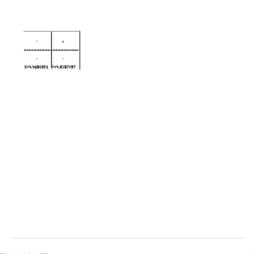
TI-83 Plus Draw Instructions 234
3. Press
Í
to draw the point.
To continue drawing points, repeat steps 2 and 3. To cancel
Pt
.
On(
,
press
‘
.
Erasing Points with Pt
.
Off(
To erase (turn off) a drawn point on a graph, follow these steps.
1. Select
2:Pt
.
Off(
(point off) from the
DRAW POINTS
menu.
2. Move the cursor to the point you want to erase.
3. Press
Í
to erase the point.
To continue erasing points, repeat steps 2 and 3. To cancel
Pt
.
Off(
,
press
‘
.

TI-83 Plus Draw Instructions 235
Changing Points with Pt
.
Change(
To change (toggle on or off) a point on a graph, follow these steps.
1. Select
3:Pt
.
Change(
(point change) from the
DRAW POINTS
menu.
2. Move the cursor to the point you want to change.
3. Press
Í
to change the point’s on/off status.
To continue changing points, repeat steps 2 and 3. To cancel
Pt
.
Change(
,
press
‘
.
Drawing Points from the Home Screen or a Program
Pt
.
On(
(point on) turns on the point at (
X
=
x
,
Y=
y
).
Pt
.
Off(
turns the point off.
Pt
.
Change(
toggles the point on or off.
mark
is optional; it determines the
point’s appearance; specify
1
,
2
, or
3
, where:
1
=
¦
(dot; default)
2
=
›
(box)
3
=
+
(cross)
Pt
.
On(
x,y[,mark]
)
Pt
.
Off(
x,y[,mark]
)
Pt
.
Change(
x,y
)
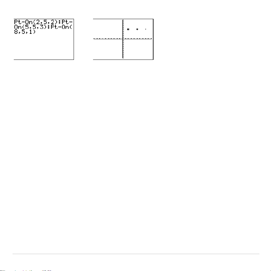
TI-83 Plus Draw Instructions 236
Note:
If you specified
mark
to turn on a point with
Pt
.
On(
, you must specify
mark
when you turn off the point with
Pt
.
Off(. Pt
.
Change(
does not have the
mark
option.

TI-83 Plus Draw Instructions 237
Drawing Pixels
TI-83 Plus Pixels
A pixel is a square dot on the TI-83 Plus display. The
Pxl
.
(pixel)
instructions let you turn on, turn off, or reverse a pixel (dot) on the graph
using the cursor. When you select a pixel instruction from the
DRAW
POINTS
menu, the TI-83 Plus returns to the home screen or the program
editor. The pixel instructions are not interactive.
Turning On and Off Pixels with Pxl
.
On( and Pxl
.
Off(
Pxl
.
On(
(pixel on) turns on the pixel at (
row
,
column
), where
row
is an
integer between 0 and 62 and
column
is an integer between 0 and 94.
Pxl
.
Off(
turns the pixel off.
Pxl
.
Change(
toggles the pixel on and off.
Pxl
.
On(
row,column
)
Pxl
.
Off(
row,column
)
Pxl
.
Change(
row,column
)

TI-83 Plus Draw Instructions 238
Using pxl
.
Test(
pxl
.
Test(
(pixel test) returns 1 if the pixel at (
row,column
) is turned on or 0 if
the pixel is turned off on the current graph.
row
must be an integer
between 0 and 62.
column
must be an integer between 0 and 94.
pxl
.
Test(
row
,
column
)
Split Screen
On a
Horiz
split screen, the maximum value for
row
is 30 for
Pxl
.
On(
,
Pxl
.
Off(
,
Pxl
.
Change(
, and
pxl
.
Test(
.
On a
G
.
T
split screen, the maximum value for
row
is 50 and the maximum
value for
column
is 46 for
Pxl
.
On(
,
Pxl
.
Off(
,
Pxl
.
Change(
, and
pxl
.
Test(
.
TI-83 Plus Draw Instructions 239
Storing Graph Pictures (Pic)
DRAW STO Menu
To display the
DRAW STO
menu, press
y
<
|
. When you select an
instruction from the
DRAW STO
menu, the TI-83 Plus returns to the home
screen or the program editor. The picture and graph database
instructions are not interactive.
DRAW POINTS STO
1: StorePic
Stores the current picture.
2: RecallPic
Recalls a saved picture.
3: StoreGDB
Stores the current graph database.
4: RecallGDB
Recalls a saved graph database.
Storing a Graph Picture
You can store up to 10 graph pictures, each of which is an image of the
current graph display, in picture variables
Pic1
through
Pic9
, or
Pic0
.
Later, you can superimpose the stored picture onto a displayed graph
from the home screen or a program.

TI-83 Plus Draw Instructions 240
A picture includes drawn elements, plotted functions, axes, and tick
marks. The picture does not include axes labels, lower and upper bound
indicators, prompts, or cursor coordinates. Any parts of the display
hidden by these items are stored with the picture.
To store a graph picture, follow these steps.
1. Select
1:StorePic
from the
DRAW STO
menu.
StorePic
is pasted to the
current cursor location.
2. Enter the number (from
1
to
9
, or
0
) of the picture variable to which
you want to store the picture. For example, if you enter
3
, the
TI-83 Plus will store the picture to
Pic3
.
Note: You also can select a variable from the
PICTURE
secondary menu
(
4
). The variable is pasted next to
StorePic
.
3. Press
Í
to display the current graph and store the picture.
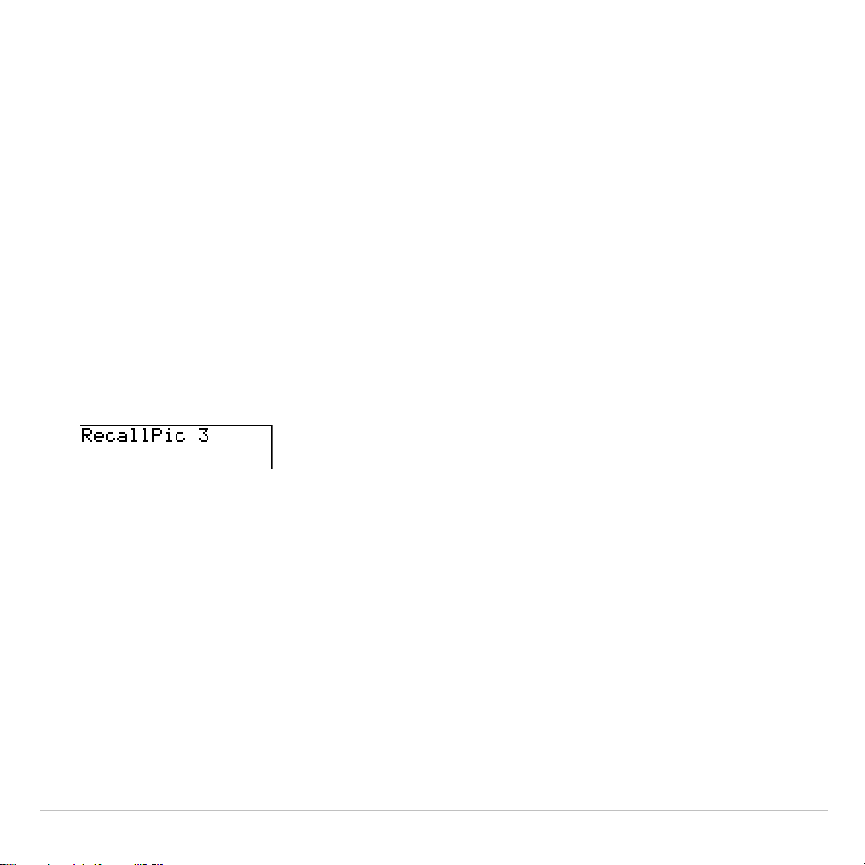
TI-83 Plus Draw Instructions 241
Recalling Graph Pictures (Pic)
Recalling a Graph Picture
To recall a graph picture, follow these steps.
1. Select
2:RecallPic
from the
DRAW STO
menu.
RecallPic
is pasted to the
current cursor location.
2. Enter the number (from
1
to
9
, or
0
) of the picture variable from which
you want to recall a picture. For example, if you enter
3
, the
TI-83 Plus will recall the picture stored to
Pic3
.
Note: You also can select a variable from the
PICTURE
secondary menu
(
4
). The variable is pasted next to
RecallPic
.
3. Press
Í
to display the current graph with the picture
superimposed on it.
Note: Pictures are drawings. You cannot trace a curve that is part of a picture.
Deleting a Graph Picture
To delete graph pictures from memory, use the
MEMORY MANAGEMENT
/DELETE
secondary menu
(Chapter 18).

TI-83 Plus Draw Instructions 242
Storing Graph Databases (GDB)
What Is a Graph Database?
A graph database (
GDB
) contains the set of elements that defines a
particular graph. You can recreate the graph from these elements. You
can store up to 10
GDB
s in variables
GDB1
through
GDB9
, or
GDB0
and
recall them to recreate graphs.
A
GDB
stores five elements of a graph.
•
Graphing mode
•
Window variables
•
Format settings
•
All functions in the
Y=
editor and the selection status of each
•
Graph style for each
Y=
function
GDB
s do not contain drawn items or stat plot definitions.
Storing a Graph Database
To store a graph database, follow these steps.
1. Select
3:StoreGDB
from the
DRAW STO
menu.
StoreGDB
is pasted to
the current cursor location.
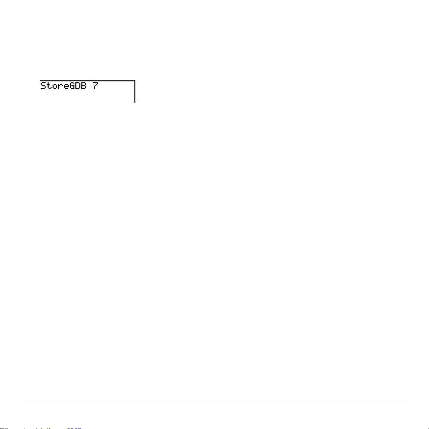
TI-83 Plus Draw Instructions 243
2. Enter the number (from
1
to
9
, or
0
) of the
GDB
variable to which you
want to store the graph database. For example, if you enter
7
, the
TI-83 Plus will store the
GDB
to
GDB7
.
Note: You also can select a variable from the
GDB
secondary menu
(
3
). The variable is pasted next to
StoreGDB
.
3. Press
Í
to store the current database to the specified
GDB
variable.
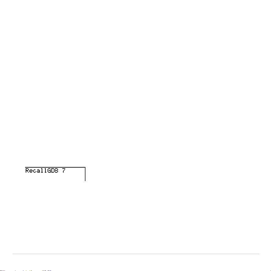
TI-83 Plus Draw Instructions 244
Recalling Graph Databases (GDB)
Recalling a Graph Database
CAUTION:
When you recall a
GDB
, it replaces all existing
Y=
functions.
Consider storing the current
Y=
functions to another database before
recalling a stored
GDB
.
To recall a graph database, follow these steps.
1. Select
4:RecallGDB
from the
DRAW STO
menu.
RecallGDB
is pasted to
the current cursor location.
2. Enter the number (from
1
to
9
, or
0
) of the
GDB
variable from which
you want to recall a
GDB
. For example, if you enter
7
, the TI-83 Plus
will recall the
GDB
stored to
GDB7
.
Note: You also can select a variable from the
GDB
secondary menu
(
3
). The variable is pasted next to
RecallGDB
.
3. Press
Í
to replace the current
GDB
with the recalled
GDB
. The
new graph is not plotted. The TI-83 Plus changes the graphing mode
automatically, if necessary.

TI-83 Plus Draw Instructions 245
Deleting a Graph Database
To delete a
GDB
from memory, use the
MEMORY MANAGEMENT/DELETE
secondary menu (Chapter 18).
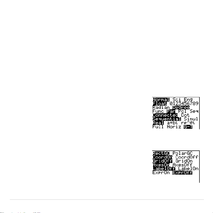
TI-83 Plus Split Screen 246
Chapter 9:
Split Screen
Getting Started: Exploring the Unit Circle
Getting Started is a fast-paced introduction. Read the chapter for details.
Use
G
.
T
(graph-table) split-screen mode to explore the unit circle and its
relationship to the numeric values for the commonly used trigonometric angles
of 0
°
, 30
°
, 45
°
, 60
°
, 90
°
, and so on.
1. Press
z
to display the mode screen. Press
†
†
~
Í
to select
Degree
mode. Press
†
~
Í
to select
Par
(parametric) graphing
mode.
Press
†
†
†
†
~
~
Í
to select
G
.
T
(graph-table) split-screen mode.
2. Press
y
.
to display the format screen.
Press
†
†
†
†
†
~
Í
to select
ExprOff
.
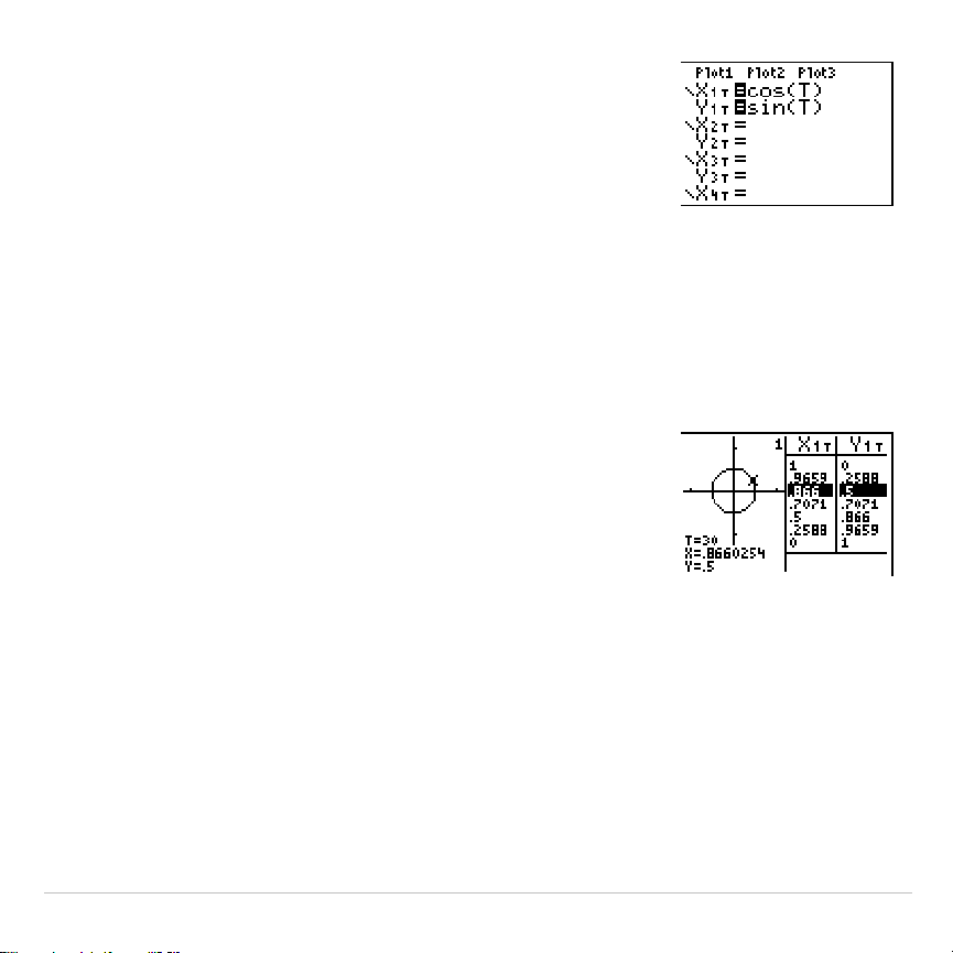
TI-83 Plus Split Screen 247
3. Press
o
to display the
Y=
editor for
Par
graphing mode. Press
™
„
¤
Í
to
store
cos(T)
to
X1T
. Press
˜
„
¤
Í
to store
sin(T)
to
Y1T
.
4. Press
p
to display the window editor.
Enter these values for the window variables.
Tmin=0 Xmin=
L
2.3 Ymin=
L
2.5
Tmax=360 Xmax=2.3 Ymax=2.5
Tstep=15 Xscl=1 Yscl=1
5. Press
r
. On the left, the unit circle is
graphed parametrically in
Degree
mode and the
trace cursor is activated. When
T=0
(from the
graph trace coordinates), you can see from the
table on the right that the value of
X1T
(
cos(T)
) is
1
and
Y1T
(
sin(T)
) is
0
. Press
~
to move the
cursor to the next 15
°
angle increment. As you
trace around the circle in steps of 15
°
, an
approximation of the standard value for each
angle is highlighted in the table.
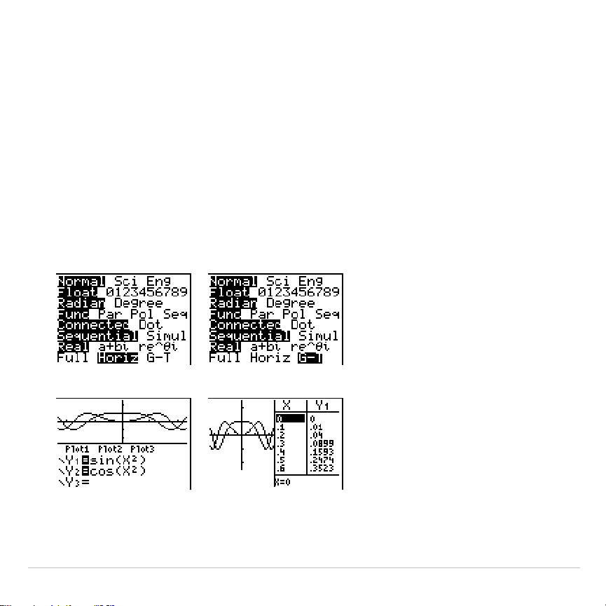
TI-83 Plus Split Screen 248
Using Split Screen
Setting a Split-Screen Mode
To set a split-screen mode, press
z
, and then move the cursor to the
bottom line of the mode screen.
•
Select
Horiz
(horizontal) to display the graph screen and another
screen split horizontally.
•
Select
G
.
T
(graph-table) to display the graph screen and table screen
split vertically.
$$
The split screen is activated when you press any key that applies to
either half of the split screen.

TI-83 Plus Split Screen 249
Some screens are never displayed as split screens. For example, if you
press
z
in
Horiz
or
G
.
T
mode, the mode screen is displayed as a full
screen. If you then press a key that displays either half of a split screen,
such as
r
, the split screen returns.
When you press a key or key combination in either
Horiz
or
G
.
T
mode,
the cursor is placed in the half of the display for which that key applies.
For example, if you press
r
, the cursor is placed in the half in which
the graph is displayed. If you press
y
0
, the cursor is placed in the
half in which the table is displayed.
The TI-83 Plus will remain in split-screen mode until you change back to
Full
screen mode.
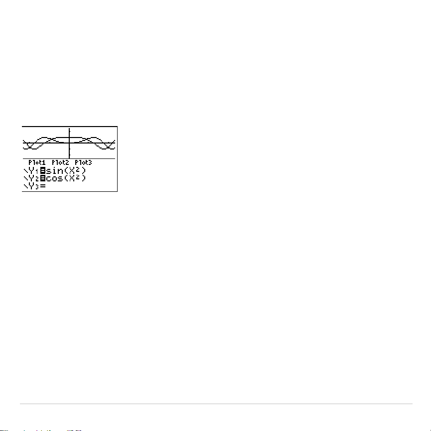
TI-83 Plus Split Screen 250
Horiz (Horizontal) Split Screen
Horiz Mode
In
Horiz
(horizontal) split-screen mode, a horizontal line splits the screen
into top and bottom halves.
The top half displays the graph.
The bottom half displays any of these editors.
•
Home screen (four lines)
•
Y=
editor (four lines)
•
Stat list editor (two rows)
•
Window editor (three settings)
•
Table editor (two rows)

TI-83 Plus Split Screen 251
Moving from Half to Half in Horiz Mode
To use the top half of the split screen:
•
Press
s
or
r
.
•
Select a
ZOOM
or
CALC
operation.
To use the bottom half of the split screen:
•
Press any key or key combination that displays the home screen.
•
Press
o
(
Y=
editor).
•
Press
…
Í
(stat list editor).
•
Press
p
(window editor).
•
Press
y
0
(table editor).
Full Screens in Horiz Mode
All other screens are displayed as full screens in
Horiz
split-screen mode.
To return to the
Horiz
split screen from a full screen when in
Horiz
mode,
press any key or key combination that displays the graph, home screen,
Y=
editor, stat list editor, window editor, or table editor.
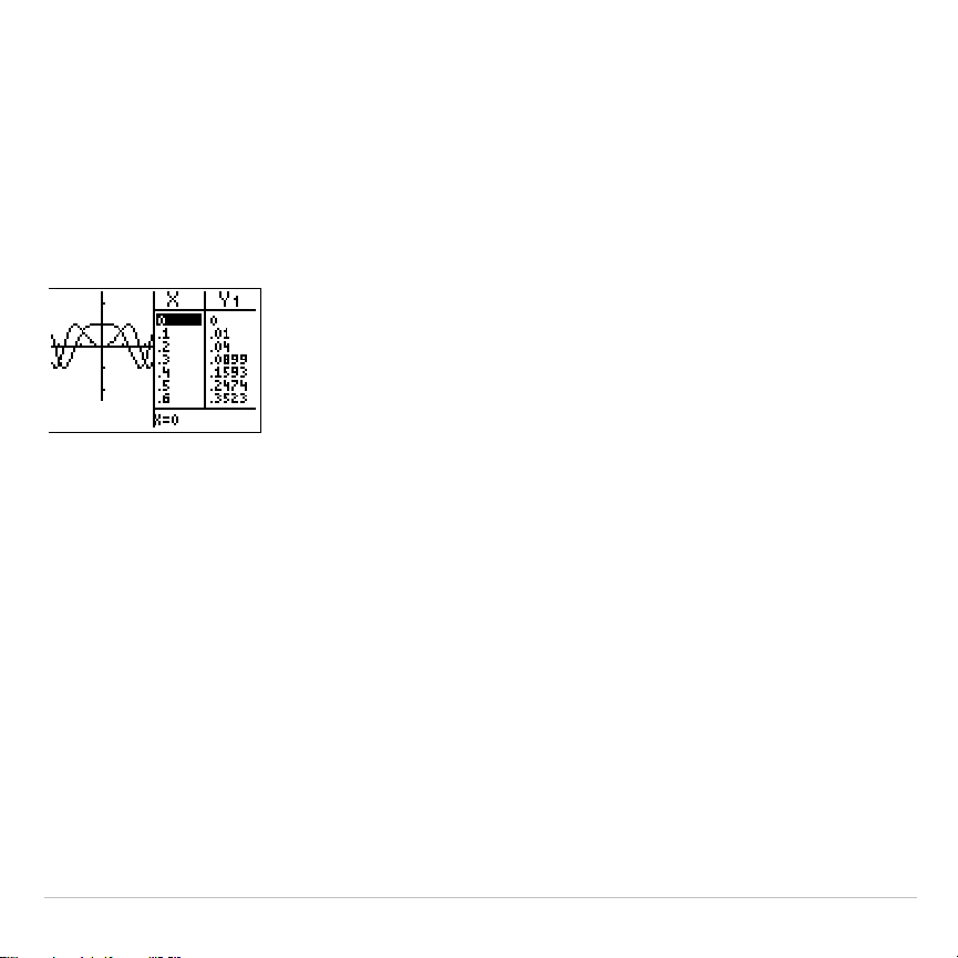
TI-83 Plus Split Screen 252
G
.
T (Graph-Table) Split Screen
G
.
T Mode
In
G
.
T
(graph-table) split-screen mode, a vertical line splits the screen
into left and right halves.
The left half displays the graph.
The right half displays the table.
Moving from Half to Half in G
.
T Mode
To use the left half of the split screen:
•
Press
s
or
r
.
•
Select a
ZOOM
or
CALC
operation.
To use the right half of the split screen, press
y
0
.
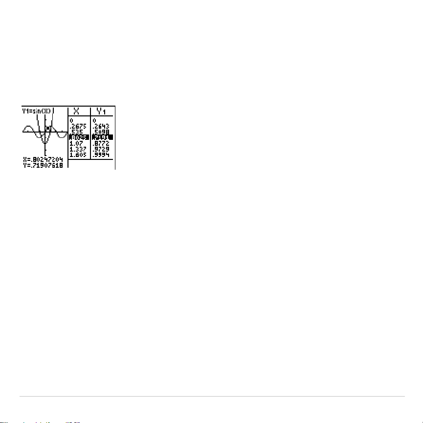
TI-83 Plus Split Screen 253
Using
r
in G
.
T Mode
As you move the trace cursor along a graph in the split screen’s left half
in
G
.
T
mode, the table on the right half automatically scrolls to match the
current cursor values.
Note: When you trace in
Par
graphing mode, both components of an equation
(
X
n
T
and
Y
n
T
) are displayed in the two columns of the table. As you trace, the
current value of the independent variable
T
is displayed on the graph.
Full Screens in G
.
T Mode
All screens other than the graph and the table are displayed as full
screens in
G
.
T
split-screen mode.
To return to the
G
.
T
split screen from a full screen when in
G
.
T
mode,
press any key or key combination that displays the graph or the table.
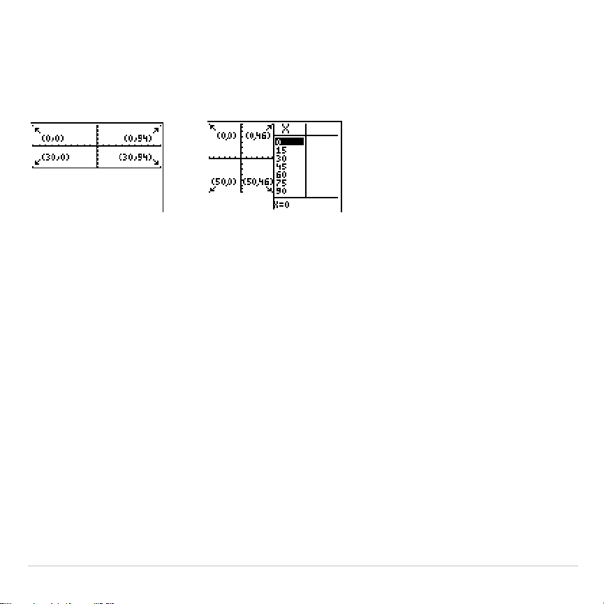
TI-83 Plus Split Screen 254
TI-83 Plus Pixels in Horiz and G
.
T Modes
TI-83 Plus Pixels in Horiz and G
.
T Modes
Note: Each set of numbers in parentheses above represents the row and
column of a corner pixel, which is turned on.
DRAW POINTS Menu Pixel Instructions
For
Pxl
.
On(
,
Pxl
.
Off(
,
Pxl
.
Change(
, and
pxl
.
Test(
:
•
In
Horiz
mode,
row
must be
{
30;
column
must be
{
94.
•
In
G
.
T
mode,
row
must be
{
50;
column
must be
{
46.
Pxl
.
On(
row
,
column
)
DRAW Menu Text( Instruction
For the
Text(
instruction:
•
In
Horiz
mode,
row
must be
{
25;
column
must be
{
94.

TI-83 Plus Split Screen 255
•
In
G
.
T
mode,
row
must be
{
45;
column
must be
{
46.
Text(
row,column,"text"
)
PRGM I/O Menu Output( Instruction
For the
Output(
instruction:
•
In
Horiz
mode,
row
must be
{
4;
column
must be
{
16.
•
In
G
.
T
mode,
row
must be
{
8;
column
must be
{
16.
Output(
row
,
column
,"
text
")
Setting a Split-Screen Mode from the Home Screen or a Program
To set
Horiz
or
G
.
T
from a program, follow these steps.
1. Press
z
while the cursor is on a blank line in the program editor.
2. Select
Horiz
or
G
.
T
.
The instruction is pasted to the cursor location. The mode is set when
the instruction is encountered during program execution. It remains in
effect after execution.
Note: You also can paste
Horiz
or
G
.
T
to the home screen or program editor
from the
CATALOG
(Chapter 15).
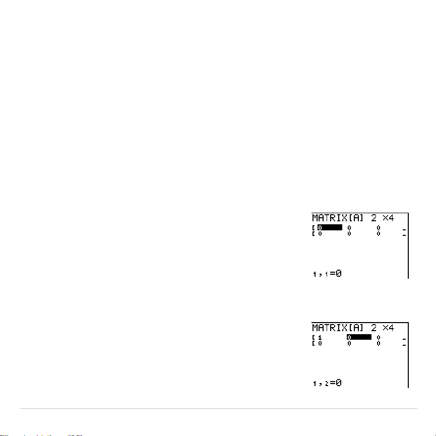
TI-83 Plus Matrices 256
Chapter 10:
Matrices
Getting Started: Systems of Linear
Equations
Getting Started is a fast-paced introduction. Read the chapter for details.
Find the solution of X + 2Y + 3Z = 3 and 2X + 3Y + 4Z = 3. On the TI-83 Plus, you
can solve a system of linear equations by entering the coefficients as elements in
a matrix, and then using
rref(
to obtain the reduced row-echelon form.
1.Press
y
>
. Press
~
~
to display the
MATRX EDIT
menu. Press
1
to select
1: [A]
¸
2.Press
2
Í
4
Í
to define a 2×4 matrix.
The rectangular cursor indicates the current
element. Ellipses (
...
) indicate additional
columns beyond the screen.
3. Press
1
Í
to enter the first element. The
rectangular cursor moves to the second column
of the first row.
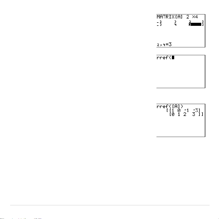
TI-83 PlusMatrices257
4.Press
2
Í
3
Í
3
Í
to complete the
first row for X + 2Y + 3Z = 3.
5.Press
2
Í
3
Í
4
Í
3
Í
to enter
the second row for 2X + 3Y + 4Z = 3.
6.Press
y
5
to return to the home screen. If
necessary, press
‘
to clear the home
screen. Press
y
>
~
to display the
MATRX MATH
menu. Press
}
to wrap to the end
of the menu. Select
B:rref(
to copy
rref(
to the
home screen.
7.Press
y
>
1
to select
1: [A]
from the
MATRX NAMES
menu. Press
¤
Í
. The
reduced row-echelon form of the matrix is
displayed and stored in
Ans
.
1X
N
1Z =
L
3 therefore X =
L
3 + Z
1Y + 2Z = 3 therefore Y = 3
N
2Z
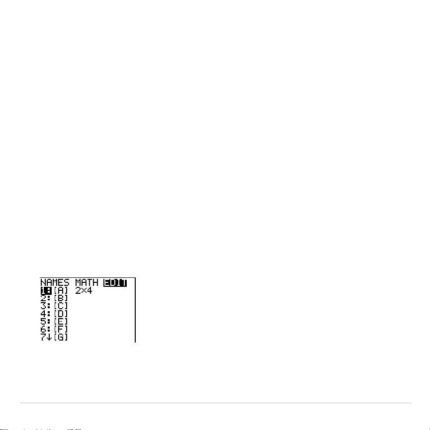
TI-83 PlusMatrices258
Defining a Matrix
What Is a Matrix?
A matrix is a two-dimensional array. You can display, define, or edit a
matrix in the matrix editor. The TI-83 Plus has 10 matrix variables,
[A]
through
[J]
. You can define a matrix directly in an expression. A matrix,
depending on available memory, may have up to 99 rows or columns.
You can store only real numbers in TI-83 Plus matrices.
Selecting a Matrix
Before you can define or display a matrix in the editor, you first must
select the matrix name. To do so, follow these steps.
1.Press
y
>
|
to display the
MATRX EDIT
menu. The dimensions
of any previously defined matrices are displayed.
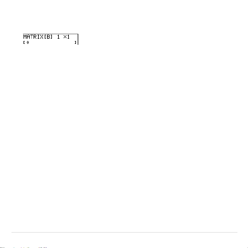
TI-83 Plus Matrices 259
2. Select the matrix you want to define. The
MATRX EDIT
screen is
displayed.
Accepting or Changing Matrix Dimensions
The dimensions of the matrix (
row
×
column
) are displayed on the top line.
The dimensions of a new matrix are
1 ×1
. You must accept or change the
dimensions each time you edit a matrix. When you select a matrix to
define, the cursor highlights the row dimension.
•
To accept the row dimension, press
Í
.
•
To change the row dimension, enter the number of rows (up to
99
),
and then press
Í
.
The cursor moves to the column dimension, which you must accept or
change the same way you accepted or changed the row dimension.
When you press
Í
, the rectangular cursor moves to the first matrix
element.
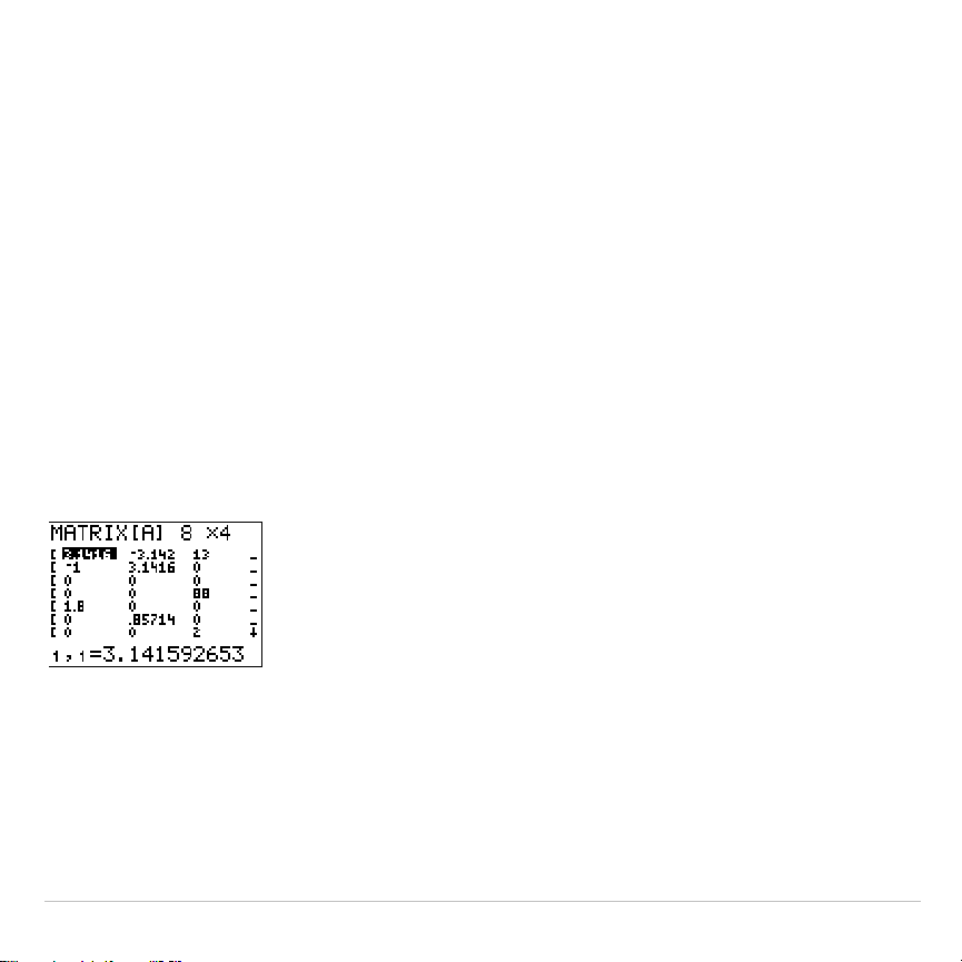
TI-83 Plus Matrices 260
Viewing and Editing Matrix Elements
Displaying Matrix Elements
After you have set the dimensions of the matrix, you can view the matrix
and enter values for the matrix elements. In a new matrix, all values are
zero.
Select the matrix from the
MATRX EDIT
menu and enter or accept the
dimensions. The center portion of the matrix editor displays up to seven
rows and three columns of a matrix, showing the values of the elements
in abbreviated form if necessary. The full value of the current element,
which is indicated by the rectangular cursor, is displayed on the bottom
line.
This is an 8 × 4 matrix. Ellipses in the left or right column indicate
additional columns.
#
or
$
in the right column indicate additional rows.
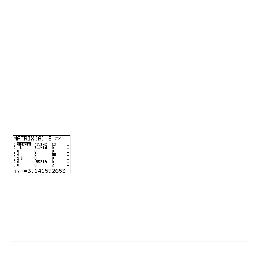
TI-83 Plus Matrices 261
Deleting a Matrix
To delete matrices from memory, use the
MEMORY MANAGEMENT/DELETE
secondary menu (Chapter 18).
Viewing a Matrix
The matrix editor has two contexts, viewing and editing. In viewing
context, you can use the cursor keys to move quickly from one matrix
element to the next. The full value of the highlighted element is displayed
on the bottom line.
Select the matrix from the
MATRX EDIT
menu, and then enter or accept the
dimensions.

TI-83 Plus Matrices 262
Viewing-Context Keys
Key Function
|
or
~
Moves the rectangular cursor within the current row
†
or
}
Moves the rectangular cursor within the current column;
on the top row,
}
moves the cursor to the column
dimension; on the column dimension,
}
moves the
cursor to the row dimension
Í
Switches to editing context; activates the edit cursor on
the bottom line
‘
Switches to editing context; clears the value on the
bottom line
Any entry character Switches to editing context; clears the value on the
bottom line; copies the character to the bottom line
y
6
Nothing
{
Nothing
Editing a Matrix Element
In editing context, an edit cursor is active on the bottom line. To edit a
matrix element value, follow these steps.
1. Select the matrix from the
MATRX EDIT
menu, and then enter or accept
the dimensions.
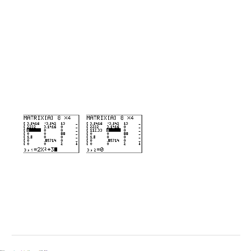
TI-83 Plus Matrices 263
2. Press
|
,
}
,
~
, and
†
to move the cursor to the matrix element you
want to change.
3. Switch to editing context by pressing
Í
,
‘
, or an entry key.
4. Change the value of the matrix element using the editing-context
keys described below. You may enter an expression, which is
evaluated when you leave editing context.
Note:
You can press
‘
Í
to restore the value at the rectangular
cursor if you make a mistake.
5. Press
Í
,
}
, or
†
to move to another element.

TI-83 Plus Matrices 264
Editing-Context Keys
Key Function
|
or
~
Moves the edit cursor within the value
†
or
}
Stores the value displayed on the bottom line to the
matrix element; switches to viewing context and moves
the rectangular cursor within the column
Í
Stores the value displayed on the bottom line to the
matrix element; switches to viewing context and moves
the rectangular cursor to the next row element
‘
Clears the value on the bottom line
Any entry character Copies the character to the location of the edit cursor on
the bottom line
y
6
Activates the insert cursor
{
Deletes the character under the edit cursor on the bottom
line

TI-83 Plus Matrices 265
Using Matrices with Expressions
Using a Matrix in an Expression
To use a matrix in an expression, you can do any of the following.
•
Copy the name from the
MATRX NAMES
menu.
•
Recall the contents of the matrix into the expression with
y
K
(Chapter 1).
•
Enter the matrix directly (see below).
Entering a Matrix in an Expression
You can enter, edit, and store a matrix in the matrix editor. You also can
enter a matrix directly in an expression.
To enter a matrix in an expression, follow these steps.
1. Press
y
[
[
] to indicate the beginning of the matrix.
2. Press
y
[
[
] to indicate the beginning of a row.
3. Enter a value, which can be an expression, for each element in the
row. Separate the values with commas.
4. Press
y
[
]
] to indicate the end of a row.
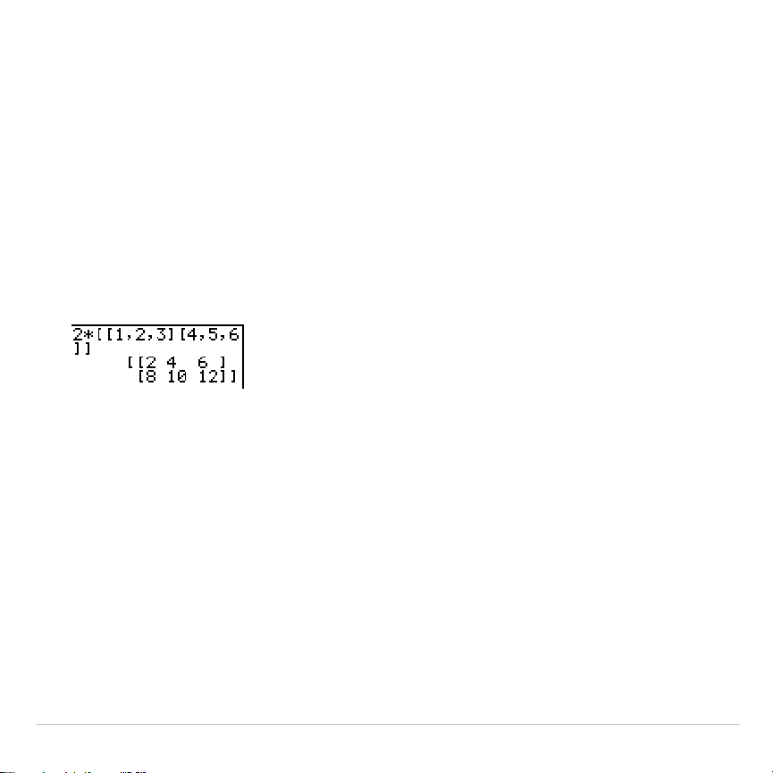
TI-83 Plus Matrices 266
5. Repeat steps 2 through 4 to enter all of the rows.
6. Press
y
[
]
] to indicate the end of the matrix.
Note: The closing
]]
are not necessary at the end of an expression or
preceding
!
.
The resulting matrix is displayed in the form:
[[
element1,1
,
...
,
element1,n
],
...
,[
elementm,1
,
...
,
elementm,n
]]
Any expressions are evaluated when the entry is executed.
Note: The commas that you must enter to separate elements are not
displayed on output.
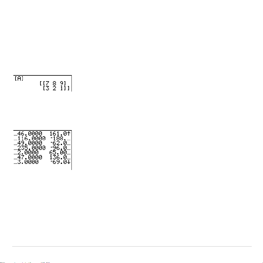
TI-83 PlusMatrices267
Displaying and Copying Matrices
Displaying a Matrix
To display the contents of a matrix on the home screen, select the matrix
from the
MATRX NAMES
menu, and then press
Í
.
Ellipses in the left or right column indicate additional columns.
#
or
$
in
the right column indicate additional rows. Press
~
,
|
,
†
, and
}
to
scroll the matrix.
Copying One Matrix to Another
To copy a matrix, follow these steps.
1.Press
y
>
to display the
MATRX NAMES
menu.
2. Select the name of the matrix you want to copy.
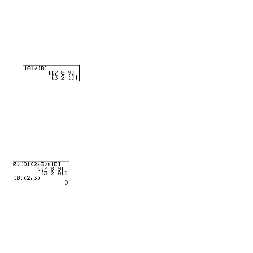
TI-83 PlusMatrices268
3.Press
¿
.
4.Press
y
>
again and select the name of the new matrix to
which you want to copy the existing matrix.
5. Press
Í
to copy the matrix to the new matrix name.
Accessing a Matrix Element
On the home screen or from within a program, you can store a value to,
or recall a value from, a matrix element. The element must be within the
currently defined matrix dimensions. Select
matrix
from the
MATRX NAMES
menu.
[
matrix
](
row
,
column
)

TI-83 Plus Matrices 269
Using Math Functions with Matrices
Using Math Functions with Matrices
You can use many of the math functions on the TI-83 Plus keyboard, the
MATH
menu, the
MATH NUM
menu, and the
MATH TEST
menu with matrices.
However, the dimensions must be appropriate. Each of the functions
below creates a new matrix; the original matrix remains the same.
+ (Add), – (Subtract),
ä
(Multiply)
To add (
Ã
) or subtract (
¹
) matrices, the dimensions must be the same.
The answer is a matrix in which the elements are the sum or difference
of the individual corresponding elements.
matrixA
+
matrixB
matrixA
N
matrixB
To multiply (
¯
) two matrices together, the column dimension of
matrixA
must match the row dimension of
matrixB
.
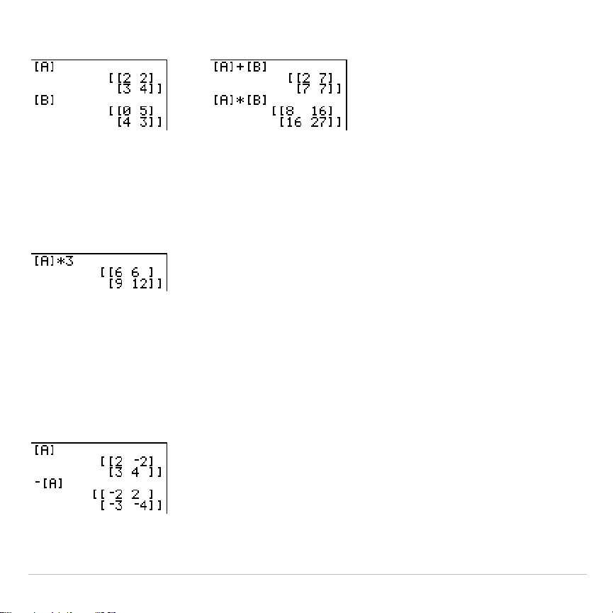
TI-83 Plus Matrices 270
matrixA
ä
matrixB
Multiplying a
matrix
by a
value
or a
value
by a
matrix
returns a matrix in
which each element of
matrix
is multiplied by
value
.
matrix
ä
value
value
ä
matrix
L
(Negation)
Negating a matrix (
Ì
) returns a matrix in which the sign of every
element is changed (reversed).
L
matrix
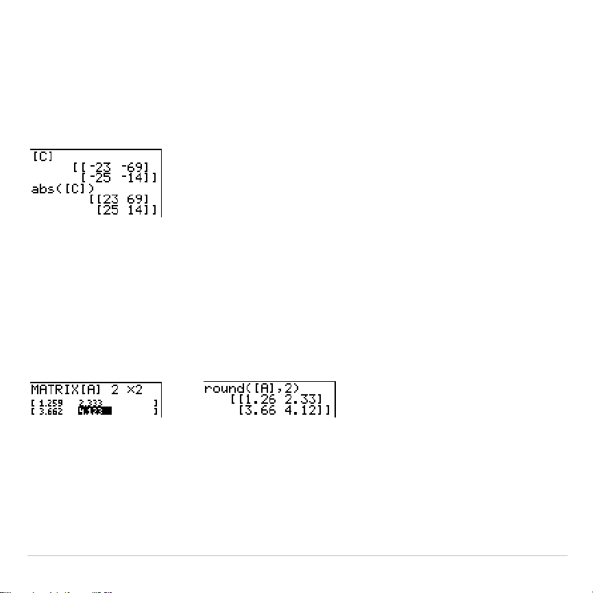
TI-83 Plus Matrices 271
abs(
abs(
(absolute value,
MATH NUM
menu) returns a matrix containing the
absolute value of each element of
matrix
.
abs(
matrix
)
round(
round(
(
MATH NUM
menu) returns a matrix. It rounds every element in
matrix
to #
decimals
(
9). If
#decimals
is omitted, the elements are rounded
to 10 digits.
round(
matrix
[
,
#decimals
]
)
M
1
(Inverse)
Use the
L
1
function (
œ
) to invert a matrix (
^
L
1
is not valid).
matrix
must be
square. The determinant cannot equal zero.
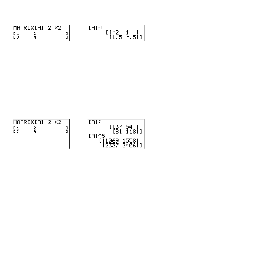
TI-83 Plus Matrices 272
matrix
L
1
Powers
To raise a matrix to a power,
matrix
must be square. You can use
2
(
¡
),
3
(
MATH
menu), or
^
power
(
›
) for integer
power
between
0
and
255
.
matrix
2
matrix
3
matrix
^
power
Relational Operations
To compare two matrices using the relational operations
=
and
ƒ
(
TEST
menu), they must have the same dimensions.
=
and
ƒ
compare
matrixA
and
matrixB
on an element-by-element basis. The other relational
operations are not valid with matrices.
matrixA
=
matrixB
returns
1
if every comparison is true; it returns
0
if any
comparison is false.
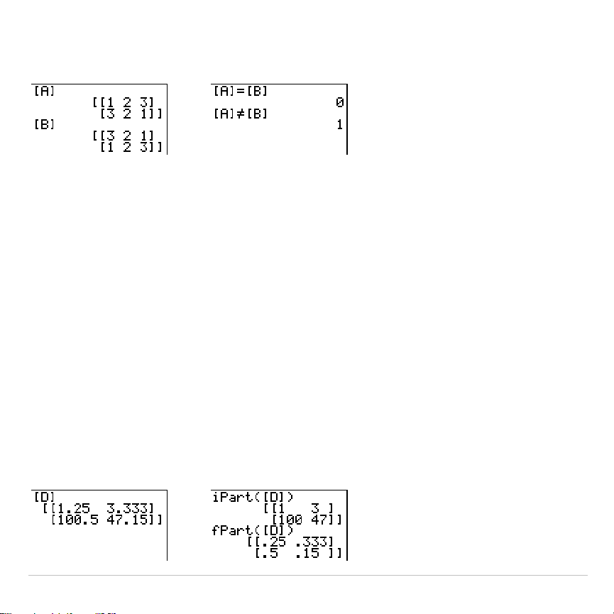
TI-83 Plus Matrices 273
matrixA
ƒ
matrixB
returns
1
if at least one comparison is false; it returns
0
if
no comparison is false.
iPart(, fPart(, int(
iPart(
(integer part),
fPart(
(fractional part), and
int(
(greatest integer) are
on the
MATH NUM
menu.
iPart(
returns a matrix containing the integer part of each element of
matrix
.
fPart(
returns a matrix containing the fractional part of each element of
matrix
.
int(
returns a matrix containing the greatest integer of each element of
matrix
.
iPart(
matrix
)
fPart(
matrix
)
int(
matrix
)
TI-83 PlusMatrices274
Using the MATRX MATH Operations
MATRX MATH Menu
To display the
MATRX MATH
menu, press
y >
~
.
NAMES MATH EDIT
1: det(
Calculates the determinant.
2:
T
Transposes the matrix.
3: dim(
Returns the matrix dimensions.
4: Fill(
Fills all elements with a constant.
5: identity(
Returns the identity matrix.
6: randM(
Returns a random matrix.
7: augment(
Appends two matrices.
8: Matr
4
list(
Stores a matrix to a list.
9: List
4
matr(
Stores a list to a matrix.
0: cumSum(
Returns the cumulative sums of a matrix.
A: ref(
Returns the row-echelon form of a matrix.
B: rref(
Returns the reduced row-echelon form.
C: rowSwap(
Swaps two rows of a matrix.
D: row+(
Adds two rows; stores in the second row.
E:
ä
row(
Multiplies the row by a number.
F:
ä
row+(
Multiplies the row, adds to the second row.
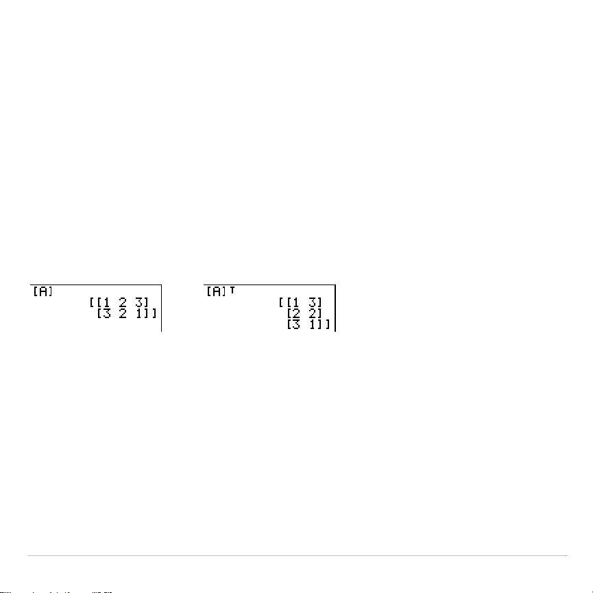
TI-83 Plus Matrices 275
det(
det(
(determinant) returns the determinant (a real number) of a square
matrix
.
det(
matrix
)
T
(Transpose)
T
(transpose) returns a matrix in which each element (row, column) is
swapped with the corresponding element (column, row) of
matrix
.
matrix
T
Accessing Matrix Dimensions with dim(
dim(
(dimension) returns a list containing the dimensions (
{
rows
columns
}
)
of
matrix
.
dim(
matrix
)
Note:
dim(
matrix
)
!
L
n
:L
n
(1)
returns the number of rows.
dim(
matrix
)
!
L
n
:L
n
(2)
returns the number of columns.
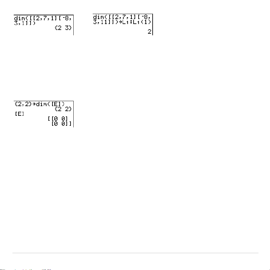
TI-83 Plus Matrices 276
Creating a Matrix with dim(
Use
dim(
with
¿
to create a new
matrixname
of dimensions
rows
×
columns
with
0
as each element.
{
rows
,
columns
}
!
dim(
matrixname
)
Redimensioning a Matrix with dim(
Use
dim(
with
¿
to redimension an existing
matrixname
to dimensions
rows
×
columns
. The elements in the old
matrixname
that are within the new
dimensions are not changed. Additional created elements are zeros.
Matrix elements that are outside the new dimensions are deleted.
{
rows
,
columns
}
!
dim(
matrixname
)
Fill(
Fill(
stores
value
to every element in
matrixname
.
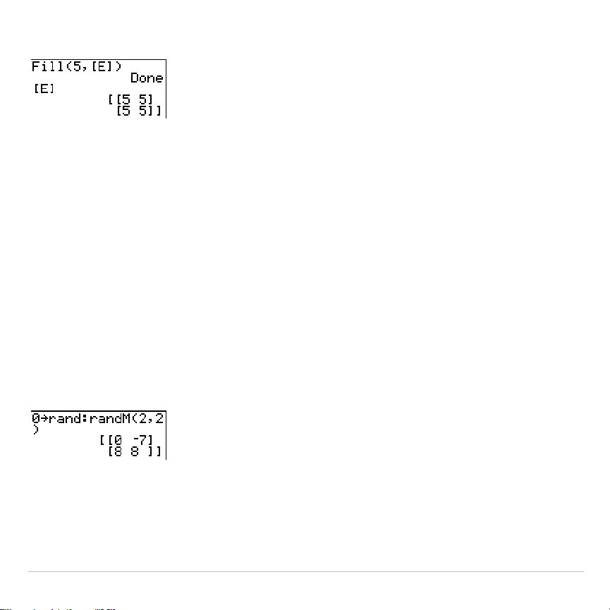
TI-83 Plus Matrices 277
Fill(
value
,
matrixname
)
identity(
identity(
returns the identity matrix of
dimension
rows ×
dimension
columns.
identity(
dimension
)
randM(
randM(
(create random matrix) returns a
rows
×
columns
random matrix of
integers
‚
L
9 and
9. The seed value stored to the
rand
function controls
the values (Chapter 2).
randM(
rows
,
columns
)
augment(
augment(
appends
matrixA
to
matrixB
as new columns.
matrixA
and
matrixB
both must have the same number of rows.
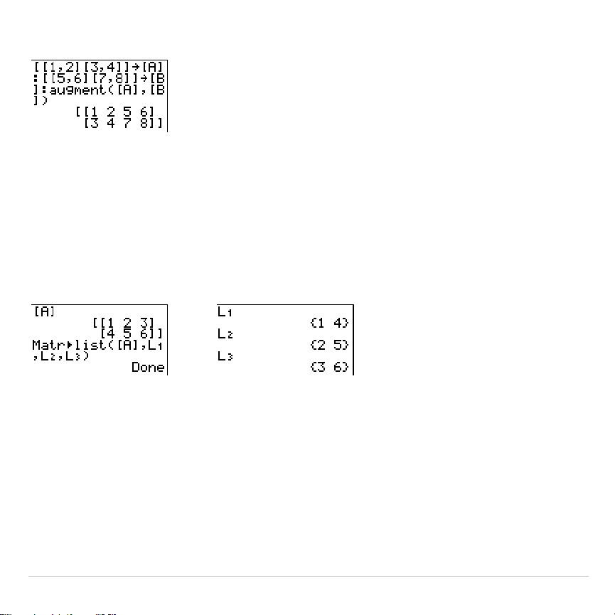
TI-83 Plus Matrices 278
augment(
matrixA
,
matrixB
)
Matr
4
list(
Matr
4
list(
(matrix stored to list) fills each
listname
with elements from each
column in
matrix
.
Matr
4
list(
ignores extra
listname
arguments. Likewise,
Matr
4
list(
ignores extra
matrix
columns.
Matr
4
list(
matrix
,
listnameA
,
...,
listname n
)
&
Matr
4
list(
also fills a
listname
with elements from a specified
column#
in
matrix
.
To fill a list with a specific column from
matrix
, you must enter
column#
after
matrix
.
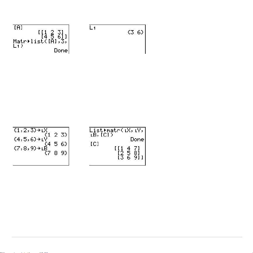
TI-83 Plus Matrices 279
Matr
4
list(
matrix
,
column#
,
listname
)
&
List
4
matr(
List
4
matr(
(lists stored to matrix) fills
matrixname
column by column with the
elements from each
list
. If dimensions of all
lists
are not equal,
List
4
matr(
fills
each extra
matrixname
row with
0
. Complex lists are not valid.
List
4
matr(
listA
,
...,
list n
,
matrixname
)
&
cumSum(
cumSum(
returns cumulative sums of the elements in
matrix
, starting with
the first element. Each element is the cumulative sum of the column from
top to bottom.
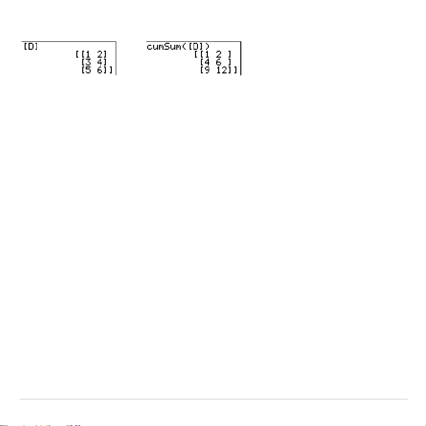
TI-83 Plus Matrices 280
cumSum(
matrix
)
Row Operations
MATRX MATH
menu items
A
through
F
are row operations. You can use a
row operation in an expression. Row operations do not change
matrix
in
memory. You can enter all row numbers and values as expressions. You
can select the matrix from the
MATRX NAMES
menu.
ref(, rref(
ref(
(row-echelon form) returns the row-echelon form of a real
matrix
. The
number of columns must be greater than or equal to the number of rows.
ref(
matrix
)
rref(
(reduced row-echelon form) returns the reduced row-echelon form of
a real
matrix
. The number of columns must be greater than or equal to the
number of rows.
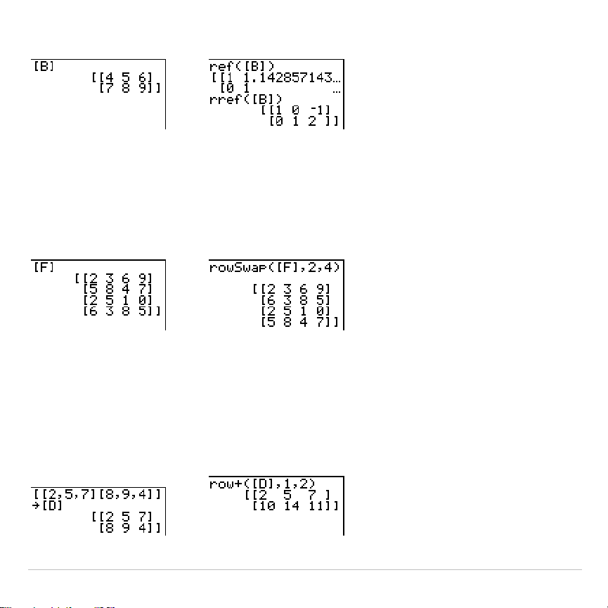
TI-83 Plus Matrices 281
rref(
matrix
)
rowSwap(
rowSwap(
returns a matrix. It swaps
rowA
and
rowB
of
matrix
.
rowSwap(
matrix
,
rowA
,
rowB
)
row+(
row+(
(row addition) returns a matrix. It adds
rowA
and
rowB
of
matrix
and
stores the results in
rowB
.
row+(
matrix
,
rowA
,
rowB
)
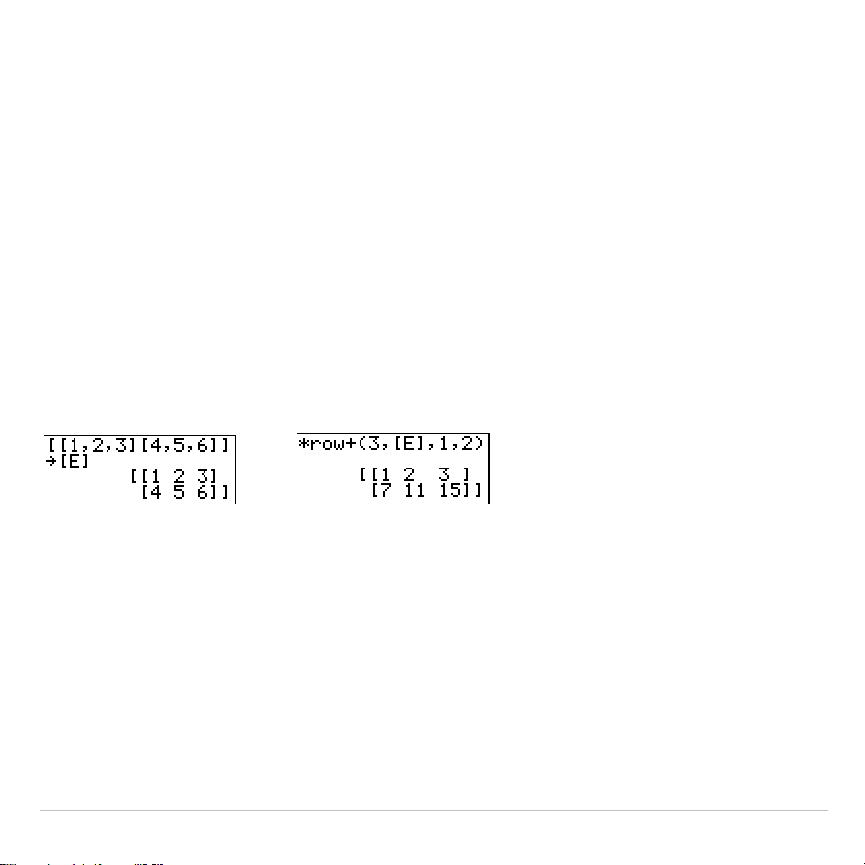
TI-83 Plus Matrices 282
ä
row(
ä
row(
(row multiplication) returns a matrix. It multiplies
row
of
matrix
by
value
and stores the results in
row
.
ä
row(
value
,
matrix
,
row
)
ä
row+(
ä
row+(
(row multiplication and addition) returns a matrix. It multiplies
rowA
of
matrix
by
value
, adds it to
rowB
, and stores the results in
rowB
.
ä
row+(
value
,
matrix
,
rowA
,
rowB
)
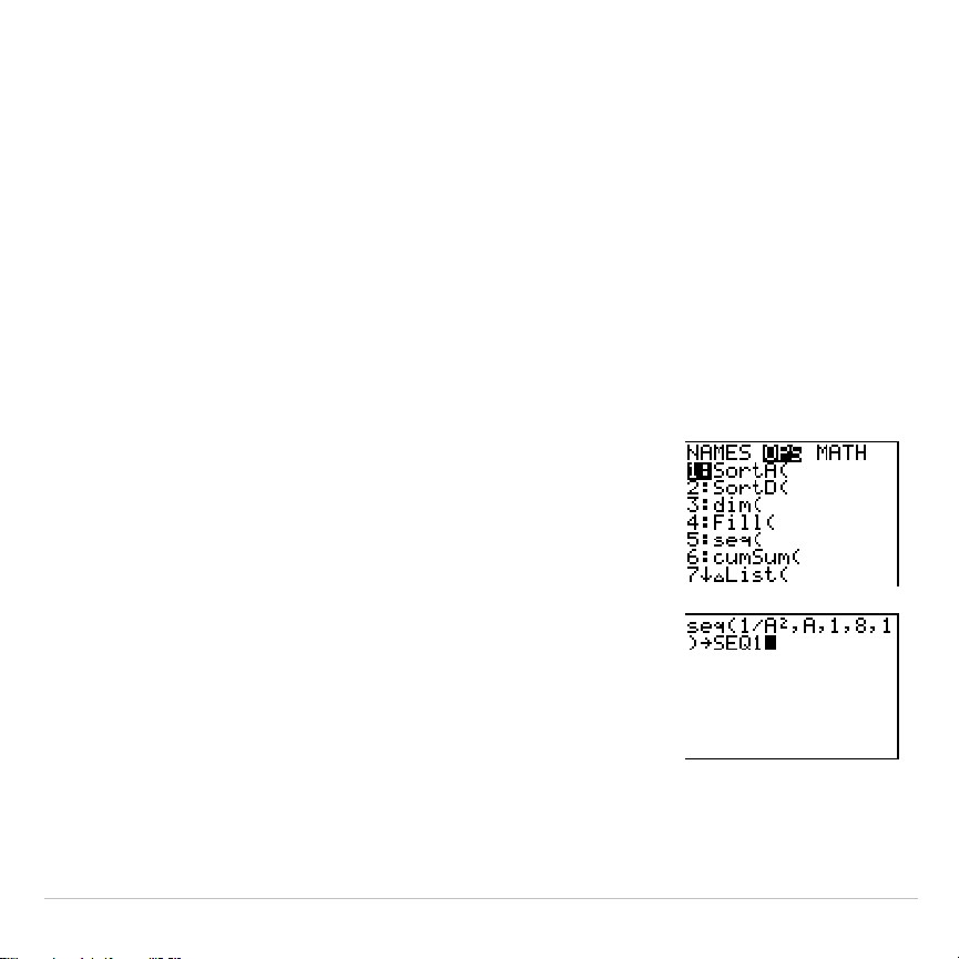
TI-83 Plus Lists 283
Chapter 11:
Lists
Getting Started: Generating a Sequence
Getting Started is a fast-paced introduction. Read the chapter for details.
Calculate the first eight terms of the sequence 1/A
2
. Store the results to a user-
created list. Then display the results in fraction form. Begin this example on a
blank line on the home screen.
1. Press
y
9
~
to display the
LIST OPS
menu.
2. Press
5
to select
5:seq(
, which pastes
seq(
to
the current cursor location.
3. Press
1
¥
ƒ
[
A
]
¡
¢
ƒ
[
A
]
¢
1
¢
8
¢
1
¤
to enter the sequence.
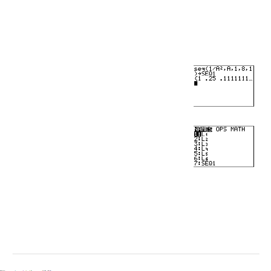
TI-83 Plus Lists 284
4. Press
¿
, and then press
y
ƒ
to turn
on alpha-lock. Press [
S
] [
E
] [
Q
], and then press
ƒ
to turn off alpha-lock. Press
1
to
complete the list name.
5. Press
Í
to generate the list and store it in
SEQ1
. The list is displayed on the home screen.
An ellipsis (
...
) indicates that the list continues
beyond the viewing window. Press
~
repeatedly (or press and hold
~
) to scroll the
list and view all the list elements.
6. Press
y
9
to display the
LIST NAMES
menu.
Press
7
to select
7:seq(
to paste
Ù
SEQ1
to the
current cursor location. (If
SEQ1
is not item
7
on
your
LIST NAMES
menu, move the cursor to
SEQ1
before you press
Í
.)
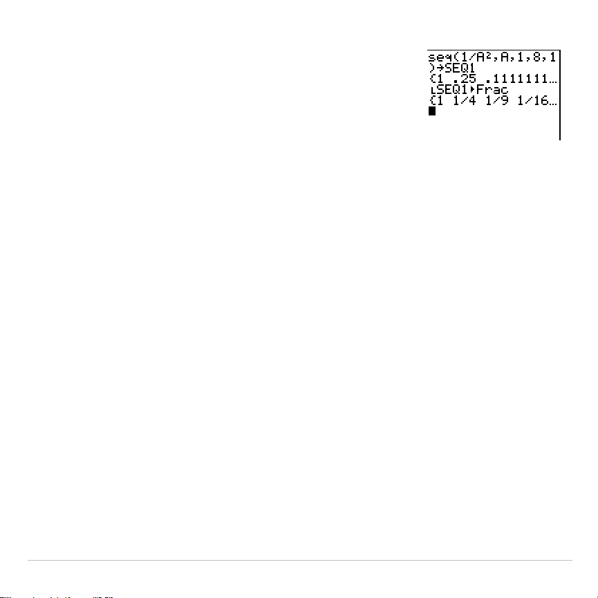
TI-83 Plus Lists 285
7. Press
to display the
MATH
menu. Press
1
to select
1:
4
Frac
, which pastes
4
Frac
to the
current cursor location.
8. Press
Í
to show the sequence in fraction
form. Press
~
repeatedly (or press and hold
~
) to scroll the list and view all the list
elements.
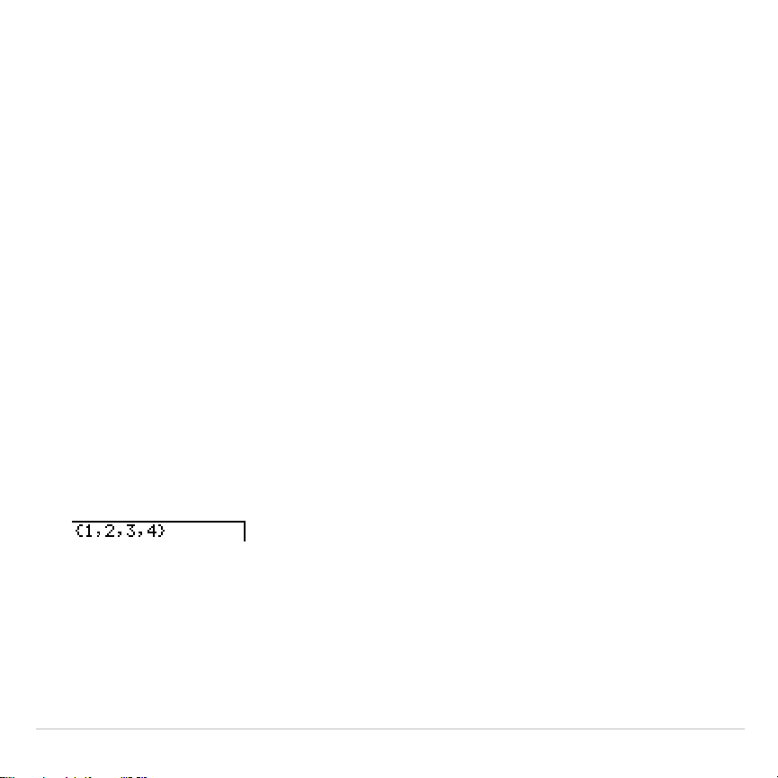
TI-83 Plus Lists 286
Naming Lists
Using TI-83 Plus List Names L
1
through L
6
The TI-83 Plus has six list names in memory:
L
1
,
L
2
,
L
3
,
L
4
,
L
5
, and
L
6
.
The list names
L
1
through
L
6
are on the keyboard above the numeric
keys
À
through
¸
. To paste one of these names to a valid screen, press
y
, and then press the appropriate key.
L
1
through
L
6
are stored in stat
list editor columns
1
through
6
when you reset memory.
Creating a List Name on the Home Screen
To create a list name on the home screen, follow these steps.
1. Press
y
E
, enter one or more list elements, and then press
y
F
.
Separate list elements with commas. List elements can be real
numbers, complex numbers, or expressions.
2. Press
¿
.
3. Press
ƒ
[
letter from A to Z or
q
] to enter the first letter of the
name.
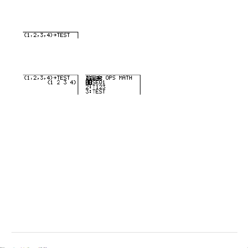
TI-83 Plus Lists 287
4. Enter zero to four letters,
q
, or numbers to complete the name.
5. Press
Í
. The list is displayed on the next line. The list name and
its elements are stored in memory. The list name becomes an item
on the
LIST NAMES
menu.
Note: If you want to view a user-created list in the stat list editor, you must
store it in the stat list editor (Chapter 12).
You also can create a list name in these four places.
•
At the
Name=
prompt in the stat list editor
•
At an
Xlist:
,
Ylist:
, or
Data List:
prompt in the stat plot editor
•
At a
List:
,
List1:
,
List2:
,
Freq:
,
Freq1:
,
Freq2:
,
XList:
, or
YList:
prompt
in the inferential stat editors
•
On the home screen using
SetUpEditor
You can create as many list names as your TI-83 Plus memory has
space to store.
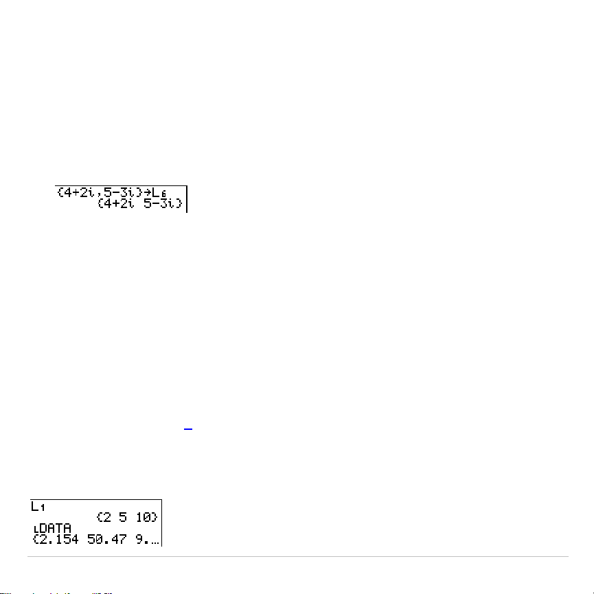
TI-83 Plus Lists 288
Storing and Displaying Lists
Storing Elements to a List
You can store list elements in either of two ways.
•
Use braces and
¿
on the home screen.
•
Use the stat list editor (Chapter 12).
The maximum dimension of a list is 999 elements.
Tip: When you store a complex number to a list, the entire list is converted to a
list of complex numbers. To convert the list to a list of real numbers, display the
home screen, and then enter
real(
listname
)
!
listname
.
Displaying a List on the Home Screen
To display the elements of a list on the home screen, enter the name of
the list (preceded by
Ù
, if necessary, and then press
Í
. An ellipsis
indicates that the list continues beyond the viewing window. Press
~
repeatedly (or press and hold
~
) to scroll the list and view all the list
elements.
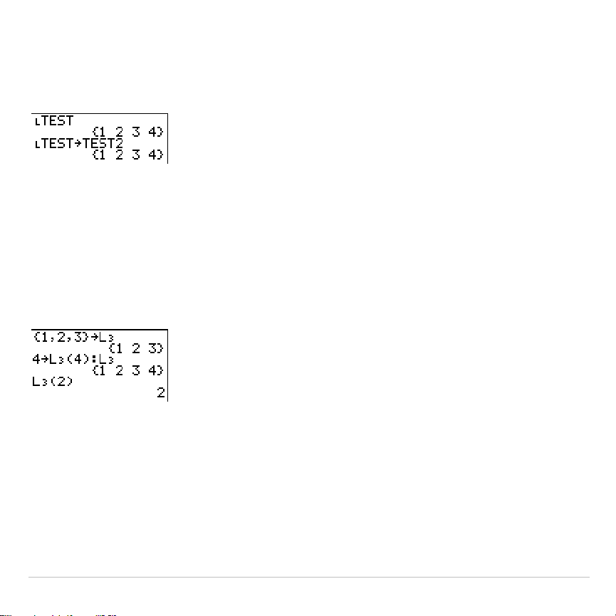
TI-83 Plus Lists 289
Copying One List to Another
To copy a list, store it to another list.
Accessing a List Element
You can store a value to or recall a value from a specific list
element
. You
can store to any element within the current list dimension or one element
beyond.
listname
(
element
)
Deleting a List from Memory
To delete lists from memory, including
L
1
through
L
6
, use the
MEMORY MANAGEMENT/DELETE
secondary menu (Chapter 18). Resetting
memory restores
L
1
through
L
6
. Removing a list from the stat list editor
does not delete it from memory.

TI-83 Plus Lists 290
Using Lists in Graphing
You can use lists to graph a family of curves (Chapter 3).
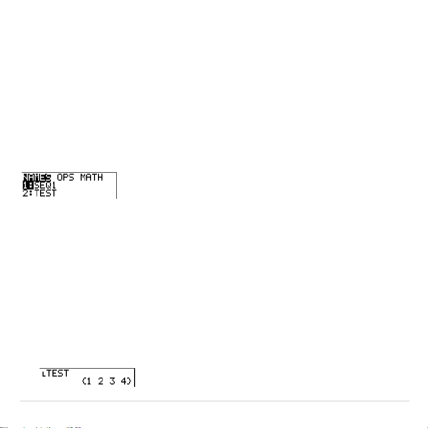
TI-83 Plus Lists 291
Entering List Names
Using the LIST NAMES Menu
To display the
LIST NAMES
menu, press
y
9
. Each item is a user-
created list name.
LIST NAMES
menu items are sorted automatically in
alphanumerical order. Only the first 10 items are labeled, using
1
through
9
, then
0
. To jump to the first list name that begins with a particular alpha
character or
q
, press
ƒ
[
letter from A to Z or
q
].
Tip: From the top of a menu, press
}
to move to the bottom. From the bottom,
press
†
to move to the top.
Note: The
LIST NAMES
menu omits list names
L1
through
L6
. Enter
L1
through
L6
directly from the keyboard.
When you select a list name from the
LIST NAMES
menu, the list name is
pasted to the current cursor location.
•
The list name symbol
Ù
precedes a list name when the name is
pasted where non-list name data also is valid, such as the home
screen.
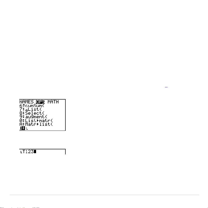
TI-83 Plus Lists 292
•
The
Ù
symbol does not precede a list name when the name is pasted
where a list name is the only valid input, such as the stat list editor’s
Name=
prompt or the stat plot editor’s
XList:
and
YList:
prompts.
Entering a User-Created List Name Directly
To enter an existing list name directly, follow these steps.
1. Press
y
9
~
to display the
LIST OPS
menu.
2. Select
B:
Ù
, which pastes
Ù
to the current cursor location.
Ù
is not
always necessary.
Note:
You also can paste
Ù
to the current
cursor location from the
CATALOG
(Chapter 15).
3. Enter the characters that comprise the list name.
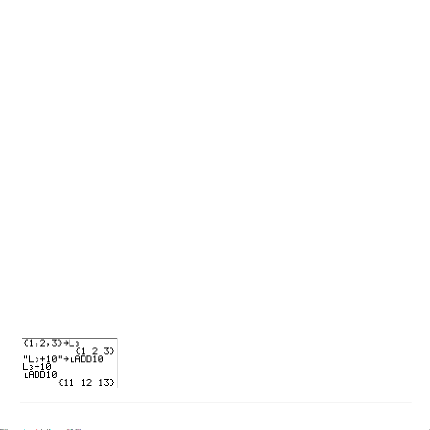
TI-83 Plus Lists 293
Attaching Formulas to List Names
Attaching a Formula to a List Name
You can attach a formula to a list name so that each list element is a
result of the formula. When executed, the attached formula must resolve
to a list.
When anything in the attached formula changes, the list to which the
formula is attached is updated automatically.
•
When you edit an element of a list that is referenced in the formula,
the corresponding element in the list to which the formula is attached
is updated.
•
When you edit the formula itself, all elements in the list to which the
formula is attached are updated.
For example, the first screen below shows that elements are stored to
L
3
, and the formula
L
3
+10
is attached to the list name
Ù
ADD10
. The
quotation marks designate the formula to be attached to
Ù
ADD10
. Each
element of
Ù
ADD10
is the sum of an element in
L
3
and 10.
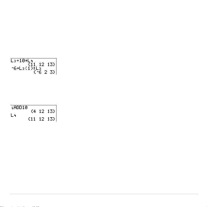
TI-83 Plus Lists 294
The next screen shows another list,
L
4
. The elements of
L
4
are the sum
of the same formula that is attached to
L
3
. However, quotation marks are
not entered, so the formula is not attached to
L
4
.
On the next line,
L
6
!
L
3
(1):L
3
changes the first element in
L
3
to
L
6
, and
then redisplays
L
3
.
The last screen shows that editing
L
3
updated
Ù
ADD10
, but did not
change
L
4
. This is because the formula
L
3
+10
is attached to
Ù
ADD10
, but
it is not attached to
L
4
.
Note:
To view a formula that is attached to a list name, use the stat list editor
(Chapter 12).
Attaching a Formula to a List on the Home Screen or in a Program
To attach a formula to a list name from a blank line on the home screen
or from a program, follow these steps.
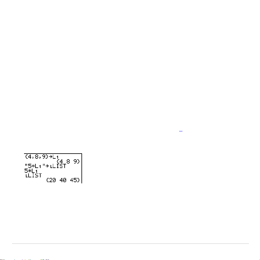
TI-83 Plus Lists 295
1. Press
ƒ
[
ã
], enter the formula (which must resolve to a list), and
press
ƒ
[
ã
] again.
Note:
When you include more than one list name in a formula, each list
must have the same dimension.
2. Press
¿
.
3. Enter the name of the list to which you want to attach the formula.
•
Press
y
, and then enter a TI-83 Plus list name
L
1
through
L
6
.
•
Press
y
9
and select a user
.
created list name from the
LIST NAMES
menu.
•
Enter a user
.
created list name directly using
Ù
.
4. Press
Í
.
Note:
The stat list editor displays a formula-lock symbol next to each list name
that has an attached formula. Chapter 12 describes how to use the stat list
editor to attach formulas to lists, edit attached formulas, and detach formulas
from lists.

TI-83 Plus Lists 296
Detaching a Formula from a List
You can detach (clear) an attached formula from a list in several ways.
For example:
•
Enter
""
!
listname
on the home screen.
•
Edit any element of a list to which a formula is attached.
•
Use the stat list editor (Chapter 12).
•
Use
ClrList
or
ClrAllList
to detach a formula from a list (Chapter 18).
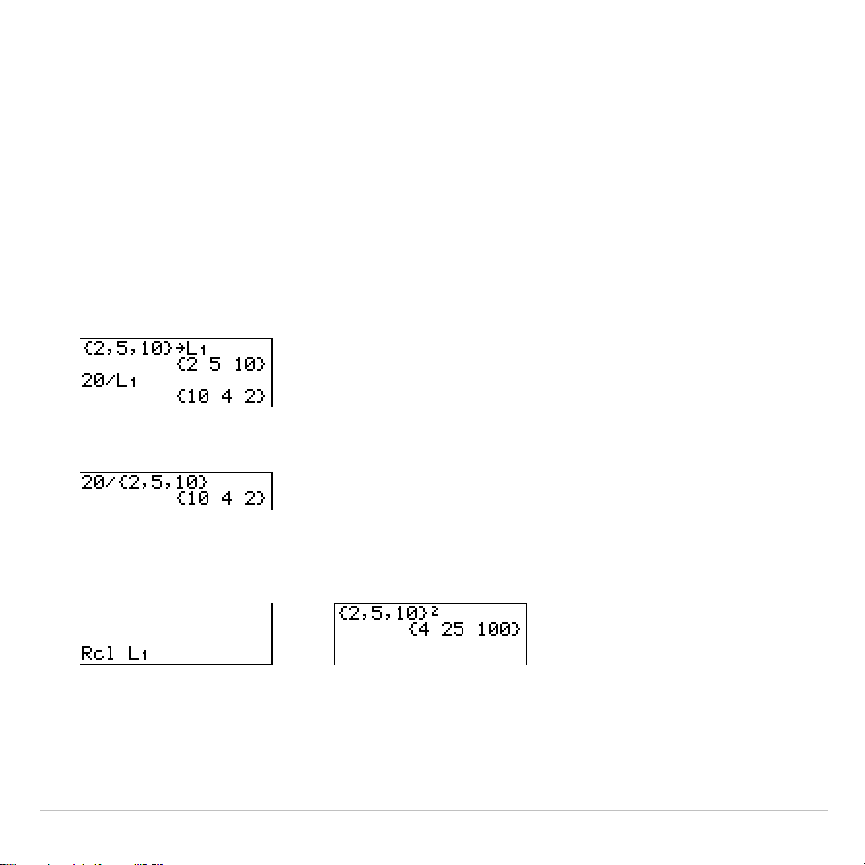
TI-83 Plus Lists 297
Using Lists in Expressions
Using a List in an Expression
You can use lists in an expression in any of three ways. When you press
Í
, any expression is evaluated for each list element, and a list is
displayed.
•
Use
L
1
–
L
6
or any user-created list name in an expression.
•
Enter the list elements directly.
•
Use
y
K
to recall the contents of the list into an expression at the
cursor location (Chapter 1).
&
Note: You must paste user-created list names to the
Rcl
prompt by selecting
them from the
LIST NAMES
menu. You cannot enter them directly using
Ù
.
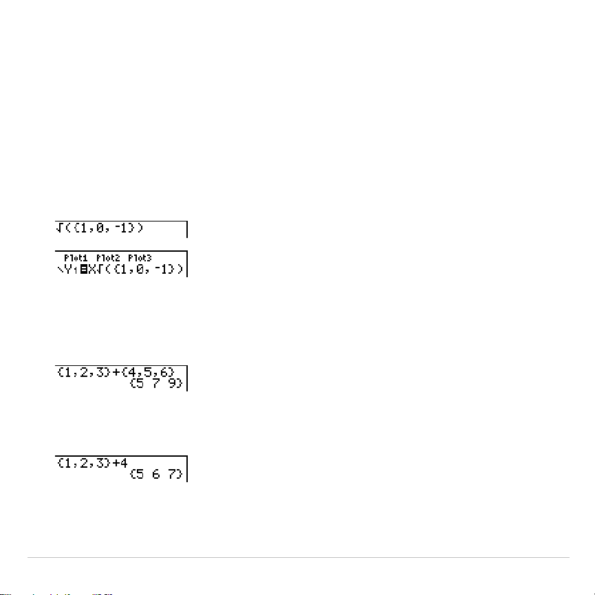
TI-83 Plus Lists 298
Using Lists with Math Functions
You can use a list to input several values for some math functions. Other
chapters and Appendix A specify whether a list is valid. The function is
evaluated for each list element, and a list is displayed.
•
When you use a list with a function, the function must be valid for
every element in the list. In graphing, an invalid element, such as
L
1
in
‡
({1,0,
L
1})
, is ignored.
This returns an error.
This graphs
X
ä
‡
(1)
and
X
ä
‡
(0)
,
but skips
X
ä
‡
(
L
1)
.
•
When you use two lists with a two-argument function, the dimension
of each list must be the same. The function is evaluated for
corresponding elements.
•
When you use a list and a value with a two-argument function, the
value is used with each element in the list.
TI-83 Plus Lists 299
LIST OPS Menu
LIST OPS Menu
To display the
LIST OPS
menu, press
y
9
~
.
NAMES OPS MATH
1: SortA(
Sorts lists in ascending order.
2: SortD(
Sorts lists in descending order.
3: dim(
Sets the list dimension.
4: Fill(
Fills all elements with a constant.
5: seq(
Creates a sequence.
6: cumSum(
Returns a list of cumulative sums.
7:
@
List(
Returns difference of successive elements.
8: Select(
Selects specific data points.
9: augment(
Concatenates two lists.
0: List
4
matr(
Stores a list to a matrix.
A: Matr
4
list(
Stores a matrix to a list.
B: Ù
Designates the list-name data type.
SortA(, SortD(
SortA(
(sort ascending) sorts list elements from low to high values.
SortD(
(sort descending) sorts list elements from high to low values.
Complex lists are sorted based on magnitude (modulus).
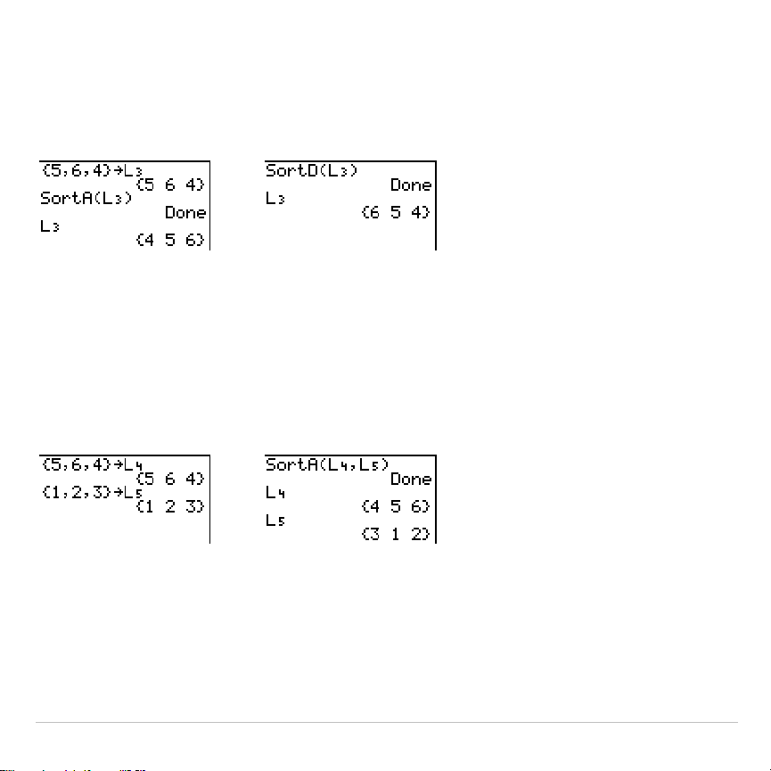
TI-83 Plus Lists 300
With one list,
SortA(
and
SortD(
sort the elements of
listname
and update
the list in memory.
SortA(
listname
) SortD(
listname
)
With two or more lists,
SortA(
and
SortD(
sort
keylistname
, and then sort
each
dependlist
by placing its elements in the same order as the
corresponding elements in
keylistname
. All lists must have the same
dimension.
SortA(
keylistname
,
dependlist1
[
,
dependlist2
,
...
,
dependlist n
]
)
SortD(
keylistname
,
dependlist1
[
,
dependlist2
,
...
,
dependlist n
]
)
Note:
In the example,
5
is the first element in
L
4
, and
1
is the first element in
L
5
. After
SortA(L
4
,L
5
)
,
5
becomes the second element of
L
4
, and likewise,
1
becomes the second element of
L
5
.
Note:
SortA(
and
SortD(
are the same as
SortA(
and
SortD(
on the
STAT EDIT
menu (Chapter 12).
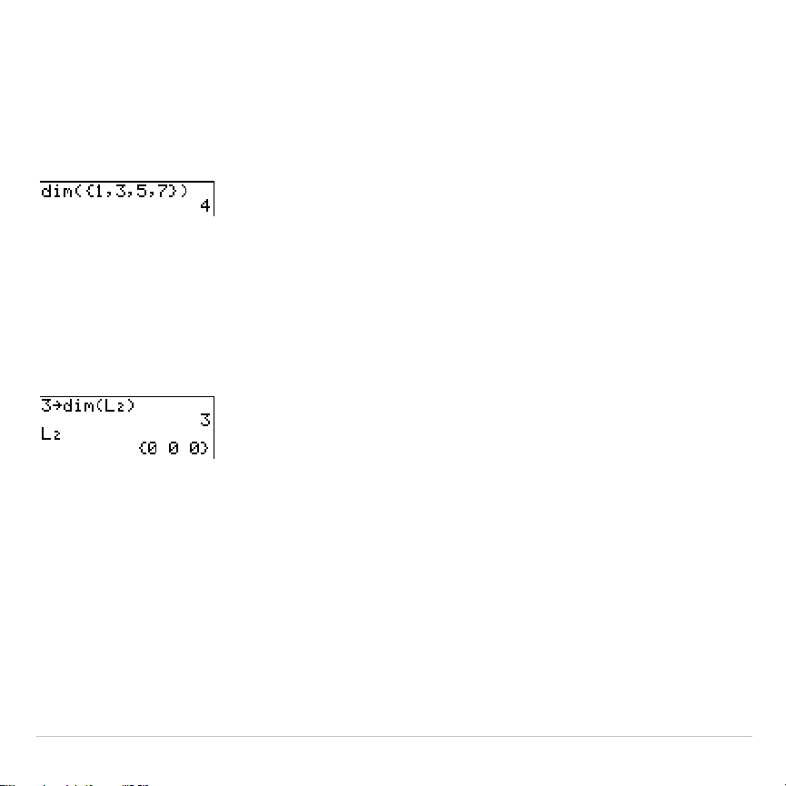
TI-83 Plus Lists 301
Using dim( to Find List Dimensions
dim(
(dimension) returns the length (number of elements) of
list
.
dim(
list
)
Using dim( to Create a List
You can use
dim(
with
¿
to create a new
listname
with dimension
length
from 1 to 999. The elements are zeros.
length
!
dim(
listname
)
Using dim( to Redimension a List
You can use
dim
with
¿
to redimension an existing
listname
to
dimension
length
from 1 to 999.
•
The elements in the old
listname
that are within the new dimension are
not changed.
•
Extra list elements are filled by
0
.
•
Elements in the old list that are outside the new dimension are deleted.
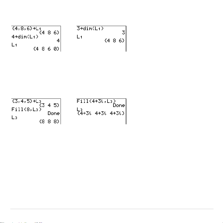
TI-83 Plus Lists 302
length
!
dim(
listname
)
Fill(
Fill(
replaces each element in
listname
with
value
.
Fill(
value
,
listname
)
Note:
dim(
and
Fill(
are the same as
dim(
and
Fill(
on the
MATRX MATH
menu
(Chapter 10).
seq(
seq(
(sequence) returns a list in which each element is the result of the
evaluation of
expression
with regard to
variable
for the values ranging from
begin
to
end
at steps of
increment
.
variable
need not be defined in memory.
increment
can be negative; the default value for
increment
is 1.
seq(
is not
valid within
expression
. Complex lists are not valid.
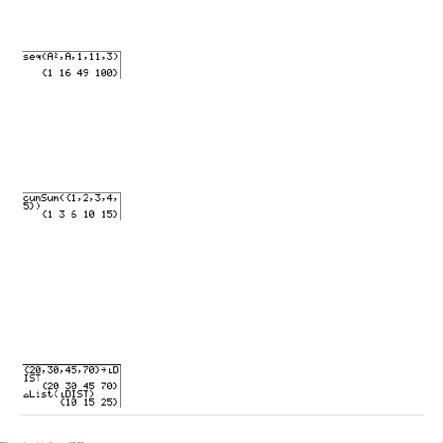
TI-83 Plus Lists 303
seq(
expression
,
variable
,
begin
,
end
[
,
increment
]
)
cumSum(
cumSum(
(cumulative sum) returns the cumulative sums of the elements
in
list
, starting with the first element.
list
elements can be real or complex
numbers.
cumSum(
list
)
@
List(
@
List(
returns a list containing the differences between consecutive
elements in
list
.
@
List
subtracts the first element in
list
from the second
element, subtracts the second element from the third, and so on. The list
of differences is always one element shorter than the original
list
.
list
elements can be a real or complex numbers.
@
List(
list
)
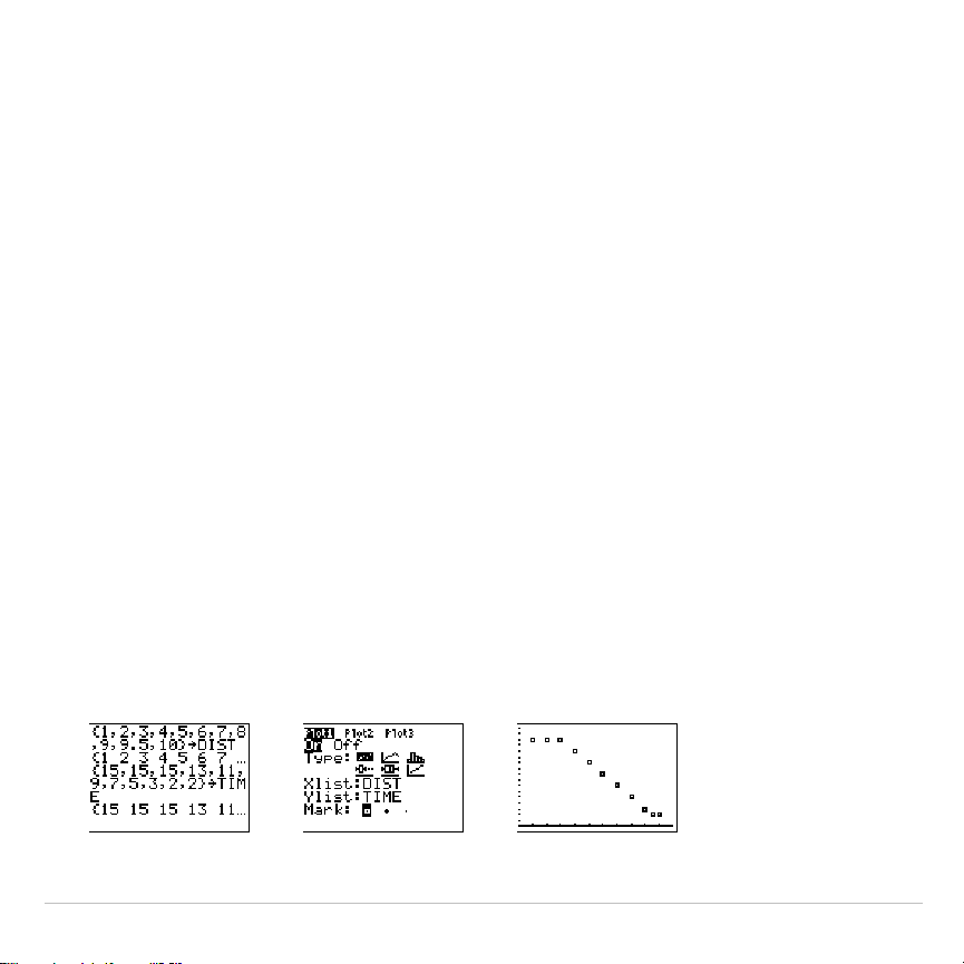
TI-83 Plus Lists 304
Select(
Select(
selects one or more specific data points from a scatter plot or
xyLine plot (only), and then stores the selected data points to two new
lists,
xlistname
and
ylistname
. For example, you can use
Select(
to select
and then analyze a portion of plotted CBL 2™/CBL™ or CBR™ data.
Select(
xlistname
,
ylistname
)
Note: Before you use
Select(
, you must have selected (turned on) a scatter plot
or xyLine plot. Also, the plot must be displayed in the current viewing window.
Before Using Select(
Before using
Select(
, follow these steps.
1. Create two list names and enter the data.
2. Turn on a stat plot, select
"
(scatter plot) or
Ó
(xyLine), and enter the
two list names for
Xlist:
and
Ylist:
(Chapter 12).
3. Use
ZoomStat
to plot the data (Chapter 3).
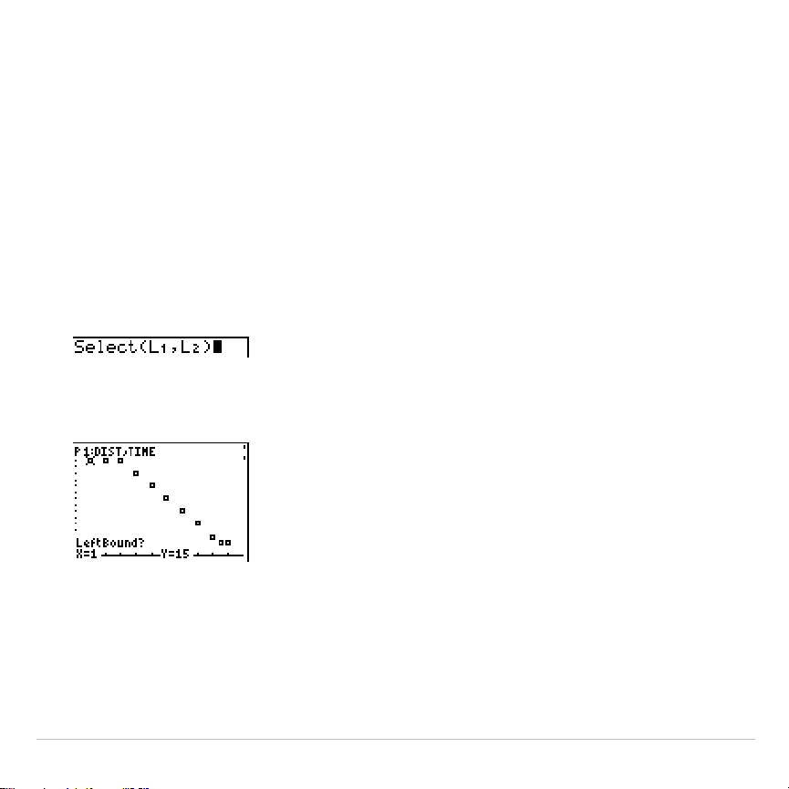
TI-83 Plus Lists 305
Using Select( to Select Data Points from a Plot
To select data points from a scatter plot or xyLine plot, follow these
steps.
1. Press
y
9
~
8
to select
8:Select(
from the
LIST OPS
menu.
Select(
is pasted to the home screen.
2. Enter
xlistname
, press
¢
, enter
ylistname
, and then press
¤
to
designate list names into which you want the selected data to be
stored.
3. Press
Í
. The graph screen is displayed with
Left Bound?
in the
bottom-left corner.
4. Press
}
or
†
(if more than one stat plot is selected) to move the
cursor onto the stat plot from which you want to select data points.
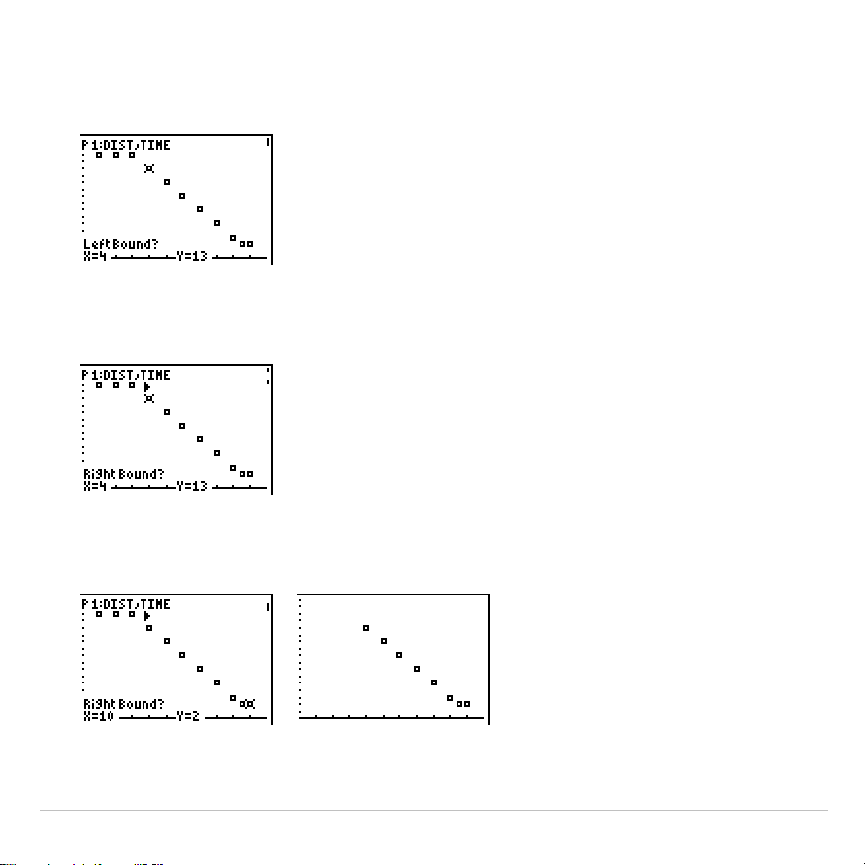
TI-83 Plus Lists 306
5. Press
|
and
~
to move the cursor to the stat plot data point that you
want as the left bound.
6. Press
Í
. A
4
indicator on the graph screen shows the left bound.
Right Bound?
is displayed in the bottom-left corner.
7. Press
|
or
~
to move the cursor to the stat plot point that you want for
the right bound, and then press
Í
.
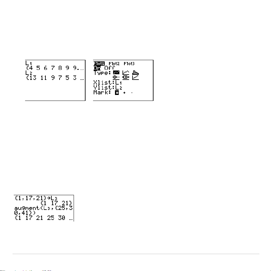
TI-83 Plus Lists 307
The x-values and y-values of the selected points are stored in
xlistname
and
ylistname
. A new stat plot of
xlistname
and
ylistname
replaces the stat plot from which you selected data points. The list
names are updated in the stat plot editor.
Note:
The two new lists (
xlistname
and
ylistname
) will include the points you
select as left bound and right bound. Also,
left-bound x-value
right-bound x-value
must be true.
augment(
augment(
concatenates the elements of
listA
and
listB
. The list elements
can be real or complex numbers.
augment(
listA
,
listB
)
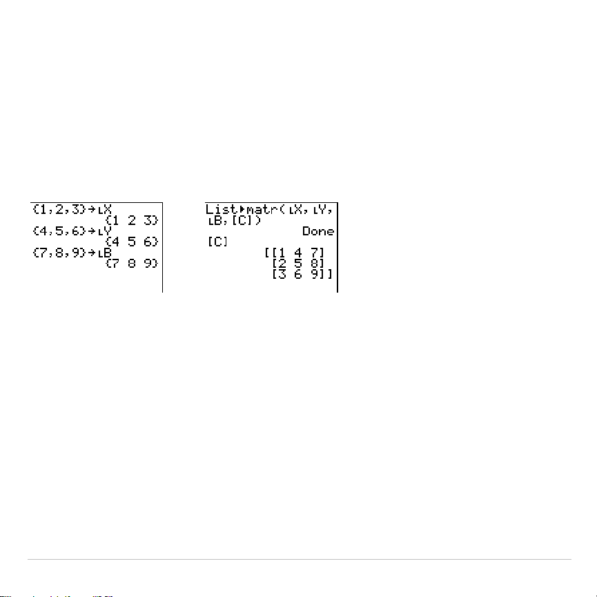
TI-83 Plus Lists 308
List
4
matr(
List
4
matr(
(lists stored to matrix) fills
matrixname
column by column with
the elements from each list. If the dimensions of all lists are not equal,
then
List
4
matr(
fills each extra
matrixname
row with
0
. Complex lists are
not valid.
List
4
matr(
list1
,
list2
,
. . .
,
list n
,
matrixname
)
&
Matr
4
list(
Matr
4
list(
(matrix stored to lists) fills each
listname
with elements from
each column in
matrix
. If the number of
listname
arguments exceeds the
number of columns in
matrix
, then
Matr
4
list(
ignores extra
listname
arguments. Likewise, if the number of columns in
matrix
exceeds the
number of
listname
arguments, then
Matr
4
list(
ignores extra
matrix
columns.
Matr
4
list(
matrix
,
listname1
,
listname2
,
. . .
,
listname n
)
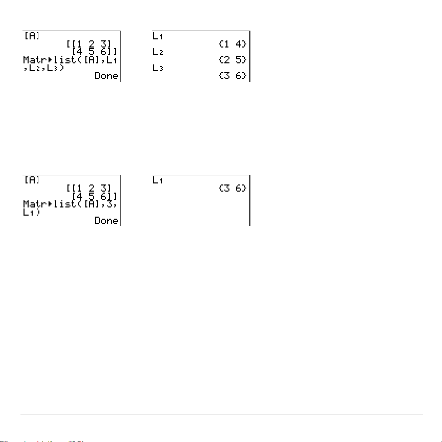
TI-83 Plus Lists 309
&
Matr
4
list(
also fills a
listname
with elements from a specified
column#
in
matrix
. To fill a list with a specific column from
matrix
, you must enter a
column#
after
matrix
.
Matr
4
list(
matrix
,
column#
,
listname
)
&
Ù
preceding one to five characters identifies those characters as a user-
created
listname
.
listname
may comprise letters,
q
, and numbers, but it
must begin with a letter from A to Z or
q
.
Ù
listname
Generally,
Ù
must precede a user-created list name when you enter a
user-created list name where other input is valid, for example, on the
home screen. Without the
Ù
, the TI-83 Plus may misinterpret a user-
created list name as implied multiplication of two or more characters.

TI-83 Plus Lists 310
Ù
need not precede a user-created list name where a list name is the
only valid input, for example, at the
Name=
prompt in the stat list editor or
the
Xlist:
and
Ylist:
prompts in the stat plot editor. If you enter
Ù
where it
is not necessary, the TI-83 Plus will ignore the entry.

TI-83 Plus Lists 311
LIST MATH Menu
LIST MATH Menu
To display the
LIST MATH
menu, press
y
9
|
.
NAMES OPS MATH
1:min(
Returns minimum element of a list.
2:max(
Returns maximum element of a list.
3:mean(
Returns mean of a list.
4:median(
Returns median of a list.
5:sum(
Returns sum of elements in a list.
6:prod(
Returns product of elements in list.
7:stdDev(
Returns standard deviation of a list.
8:variance(
Returns the variance of a list.
min(, max(
min(
(minimum) and
max(
(maximum) return the smallest or largest
element of
listA
. If two lists are compared, it returns a list of the smaller or
larger of each pair of elements in
listA
and
listB
. For a complex list, the
element with smallest or largest magnitude (modulus) is returned.
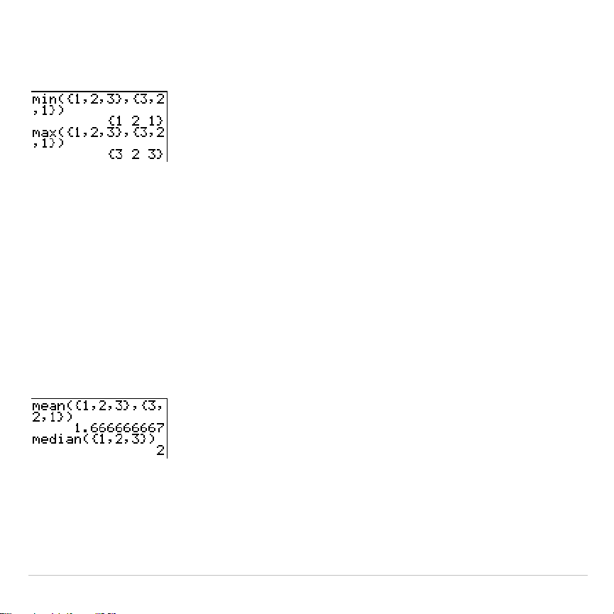
TI-83 Plus Lists 312
min(
listA
[
,
listB
]
)
max(
listA
[
,
listB
]
)
Note:
min(
and
max(
are the same as
min(
and
max(
on the
MATH NUM
menu.
mean(, median(
mean(
returns the mean value of
list
.
median(
returns the median value of
list
. The default value for
freqlist
is 1. Each
freqlist
element counts the
number of consecutive occurrences of the corresponding element in
list
.
Complex lists are not valid.
mean(
list
[
,
freqlist
]
)
median(
list
[
,
freqlist
]
)
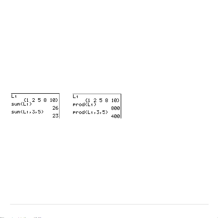
TI-83 Plus Lists 313
sum(, prod(
sum(
(summation) returns the sum of the elements in
list
.
start
and
end
are
optional; they specify a range of elements.
list
elements can be real or
complex numbers.
prod(
returns the product of all elements of
list
.
start
and
end
elements are
optional; they specify a range of list elements.
list
elements can be real
or complex numbers.
sum(
list
[
,
start
,
end
]
) prod(
list
[
,
start
,
end
]
)
Sums and Products of Numeric Sequences
You can combine
sum(
or
prod(
with
seq(
to obtain:
upper upper
G
expression(x)
∏
expression(x)
x=lower x=lower
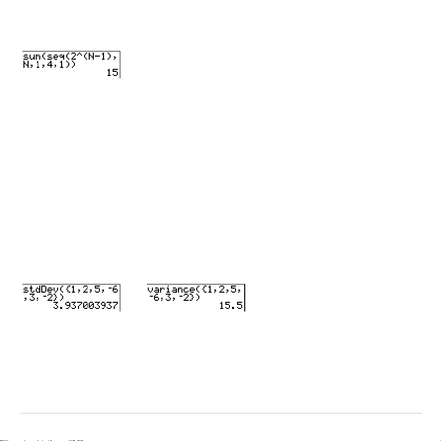
TI-83 Plus Lists 314
To evaluate
G
2
(N–1)
from N=1 to 4:
stdDev(, variance(
stdDev(
returns the standard deviation of the elements in
list
. The default
value for
freqlist
is 1. Each
freqlist
element counts the number of
consecutive occurrences of the corresponding element in
list
. Complex lists
are not valid.
variance(
returns the variance of the elements in
list
. The default value for
freqlist
is 1. Each
freqlist
element counts the number of consecutive
occurrences of the corresponding element in
list
. Complex lists are not
valid.
stdDev(
list
[
,
freqlist
]
) variance(
list
[
,
freqlist
]
)

TI-83 Plus Statistics 315
Chapter 12:
Statistics
Getting Started: Pendulum Lengths and
Periods
Getting Started is a fast-paced introduction. Read the chapter for details.
A group of students is attempting to determine the mathematical relationship
between the length of a pendulum and its period (one complete swing of a
pendulum). The group makes a simple pendulum from string and washers and
then suspends it from the ceiling. They record the pendulum’s period for each of
12 string lengths.*
Length (cm) Time (sec) Length (cm) Time (sec)
6.5 0.51 24.4 1.01
11.0 0.68 26.6 1.08
13.2 0.73 30.5 1.13
15.0 0.79 34.3 1.26
18.0 0.88 37.6 1.28
23.1 0.99 41.5 1.32
*
This example is quoted and adapted from
Contemporary Precalculus Through
Applications
, by the North Carolina School of Science and Mathematics, by permission
of Janson Publications, Inc., Dedham, MA. 1-800-322-MATH. © 1992. All rights
reserved.
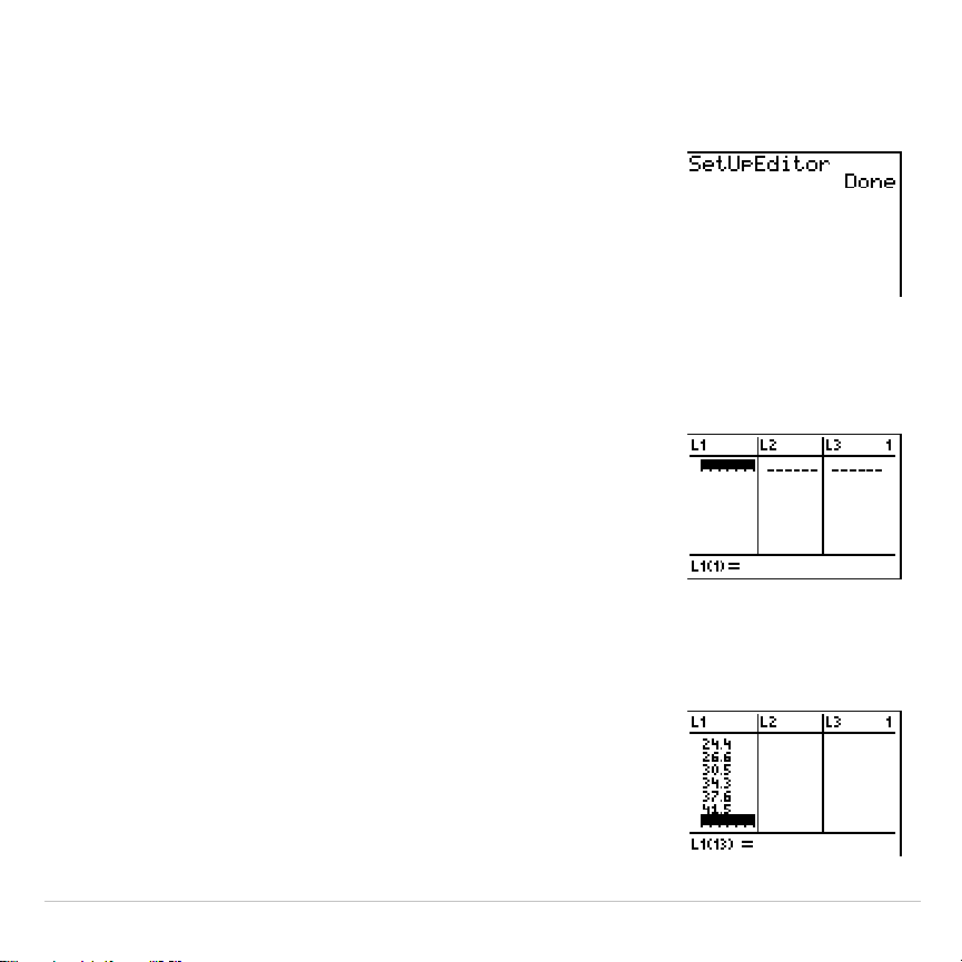
TI-83 Plus Statistics 316
1. Press
z
†
†
†
Í
to set
Func
graphing
mode.
2. Press
…
5
to select
5:SetUpEditor
.
SetUpEditor
is pasted to the home screen.
Press
Í
. This removes lists from stat list
editor columns
1
through
20
, and then stores
lists
L1
through
L6
in columns
1
through
6
.
Note: Removing lists from the stat list editor does
not delete them from memory.
3. Press
…
1
to select
1:Edit
from the
STAT
EDIT
menu. The stat list editor is displayed.
If elements are stored in
L1
and
L2
, press
}
to move the cursor onto
L1
, and then
press
‘
Í
~
}
‘
Í
to
clear both lists. Press
|
to move the
rectangular cursor back to the first row in
L1
.
4. Press
6
Ë
5
Í
to store the first pendulum
string length (6.5 cm) in
L1
. The rectangular
cursor moves to the next row. Repeat this step
to enter each of the 12 string length values in
the table.
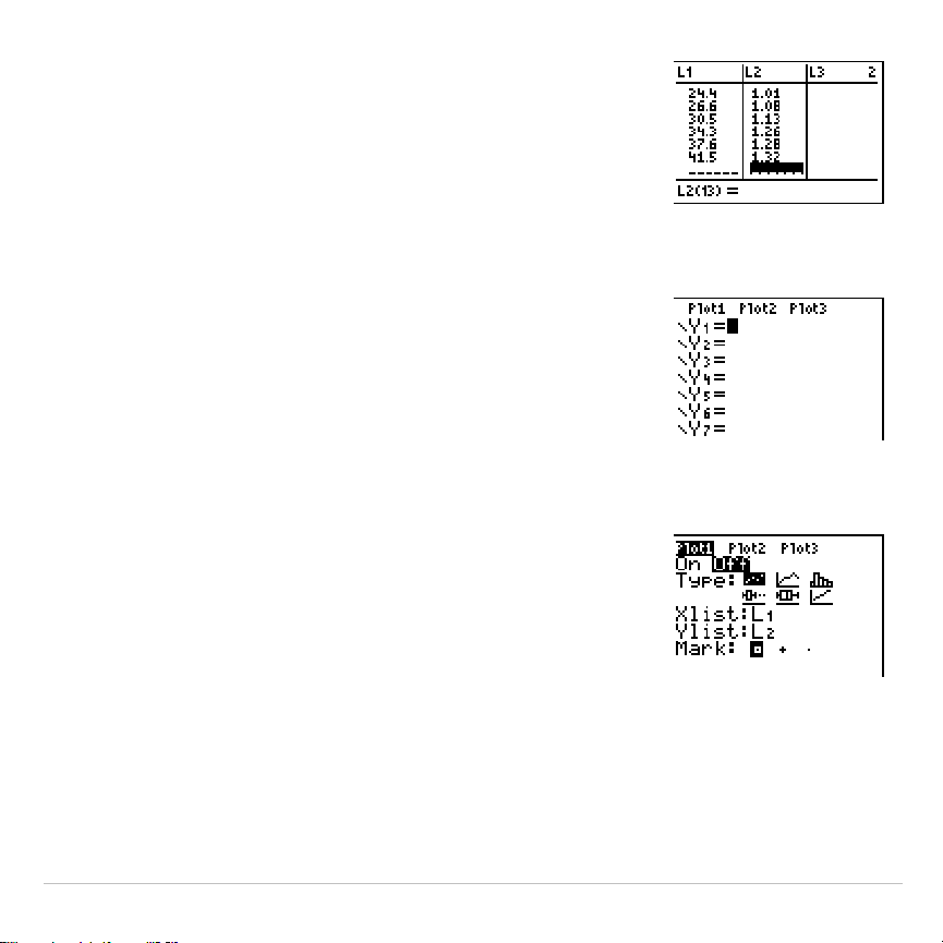
TI-83 Plus Statistics 317
5. Press
~
to move the rectangular cursor to the
first row in
L2
.
Press
Ë
51
Í
to store the first time
measurement (.51 sec) in
L2
. The rectangular
cursor moves to the next row. Repeat this step
to enter each of the 12 time values in the table.
6. Press
o
to display the
Y=
editor.
If necessary, press
‘
to clear the function
Y1
. As necessary, press
}
,
Í
, and
~
to turn
off
Plot1
,
Plot2
, and
Plot3
from the top line of the
Y=
editor (Chapter 3). As necessary, press
†
,
|
,
and
Í
to deselect functions.
7. Press
y
,
1
to select
1:Plot1
from the
STAT PLOTS
menu. The stat plot editor is
displayed for plot 1.
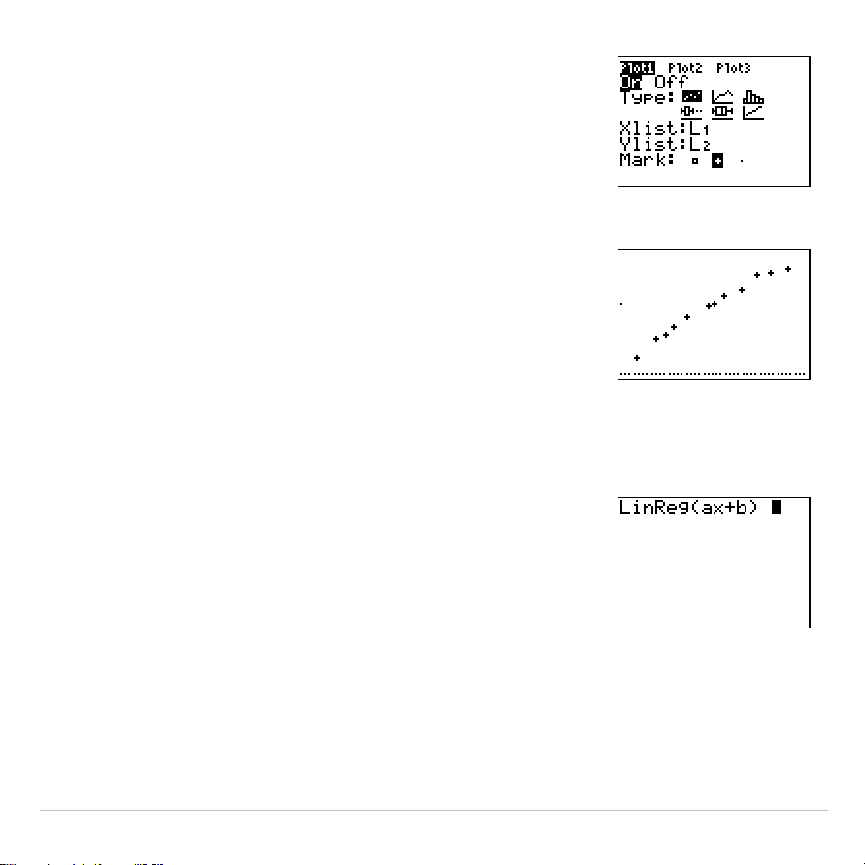
TI-83 Plus Statistics 318
8. Press
Í
to select
On
, which turns on plot 1.
Press
†
Í
to select
"
(scatter plot). Press
†
y
d
to specify
Xlist:L1
for plot 1. Press
†
y
e
to specify
Ylist:L2
for plot 1. Press
†
~
Í
to select
+
as the
Mark
for each data point
on the scatter plot.
9. Press
q
9
to select
9:ZoomStat
from the
ZOOM
menu. The window variables are adjusted
automatically, and plot 1 is displayed. This is a
scatter plot of the time-versus-length data.
Since the scatter plot of time-versus-length data appears to be
approximately linear, fit a line to the data.
10. Press
…
~
4
to select
4:LinReg(ax+b)
(linear
regression model) from the
STAT CALC
menu.
LinReg(ax+b)
is pasted to the home screen.

TI-83 Plus Statistics 319
11. Press
y
d
¢
y
e
¢
. Press
~
1
to
display the
VARS Y
.
VARS FUNCTION
secondary
menu, and then press
1
to select
1:Y1
.
L1
,
L2
,
and
Y1
are pasted to the home screen as
arguments to
LinReg(ax+b)
.
12. Press
Í
to execute
LinReg(ax+b)
. The linear
regression for the data in
L1
and
L2
is calculated.
Values for
a
and
b
are displayed on the home
screen. The linear regression equation is stored
in
Y1
. Residuals are calculated and stored
automatically in the list name
RESID
, which
becomes an item on the
LIST NAMES
menu.
13. Press
s
. The regression line and the
scatter plot are displayed.
The regression line appears to fit the central portion of the scatter plot
well. However, a residual plot may provide more information about this
fit.
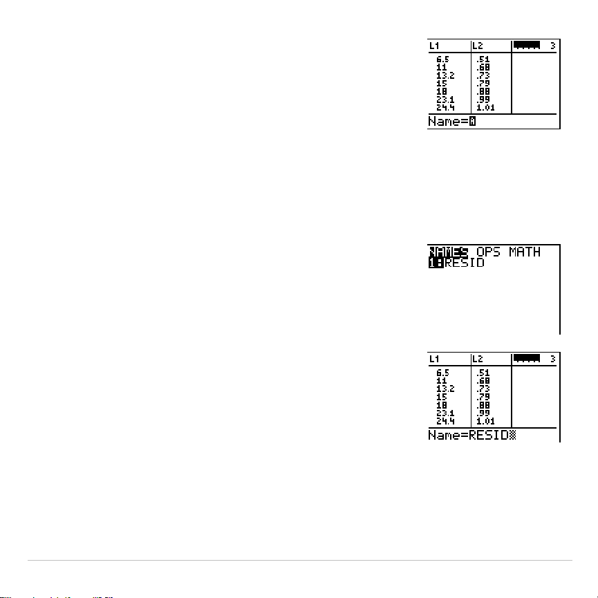
TI-83 Plus Statistics 320
14. Press
…
1
to select
1:Edit
. The stat list
editor is displayed.
Press
~
and
}
to move the cursor onto
L3
.
Press
y
6
. An unnamed column is
displayed in column
3
;
L3
,
L4
,
L5
, and
L6
shift
right one column. The
Name=
prompt is
displayed in the entry line, and alpha-lock is
on.
15. Press
y
9
to display the
LIST NAMES
menu.
If necessary, press
†
to move the cursor onto
the list name
RESID
.
16. Press
Í
to select
RESID
and paste it to the
stat list editor’s
Name=
prompt.
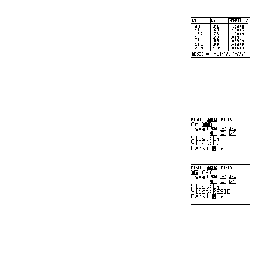
TI-83 Plus Statistics 321
17. Press
Í
.
RESID
is stored in column
3
of the
stat list editor.
Press
†
repeatedly to examine the residuals.
Notice that the first three residuals are negative. They correspond to the
shortest pendulum string lengths in
L1
. The next five residuals are
positive, and three of the last four are negative. The latter correspond to
the longer string lengths in
L1
. Plotting the residuals will show this pattern
more clearly.
18. Press
y
,
2
to select
2:Plot2
from the
STAT PLOTS
menu. The stat plot editor is
displayed for plot 2.
19. Press
Í
to select
On
, which turns on plot 2.
Press
†
Í
to select
"
(scatter plot). Press
†
y
d
to specify
Xlist:L1
for plot 2. Press
†
[
R
] [
E
] [
S
] [
I
] [
D
] (alpha-lock is on) to specify
Ylist:RESID
for plot 2. Press
†
Í
to select
›
as the mark for each data point on the
scatter plot.
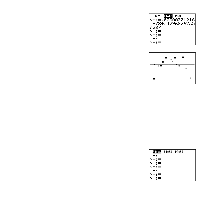
TI-83 Plus Statistics 322
20. Press
o
to display the
Y=
editor.
Press
|
to move the cursor onto the
=
sign,
and then press
Í
to deselect
Y1
. Press
}
Í
to turn off plot 1.
21. Press
q
9
to select
9:ZoomStat
from the
ZOOM
menu. The window variables are
adjusted automatically, and plot 2 is displayed.
This is a scatter plot of the residuals.
Notice the pattern of the residuals: a group of negative residuals, then a
group of positive residuals, and then another group of negative residuals.
The residual pattern indicates a curvature associated with this data set
for which the linear model did not account. The residual plot emphasizes
a downward curvature, so a model that curves down with the data would
be more accurate. Perhaps a function such as square root would fit. Try
a power regression to fit a function of the form y = a
ä
x
b
.
22. Press
o
to display the
Y=
editor.
Press
‘
to clear the linear regression
equation from
Y1
. Press
}
Í
to turn on
plot 1. Press
~
Í
to turn off plot 2.
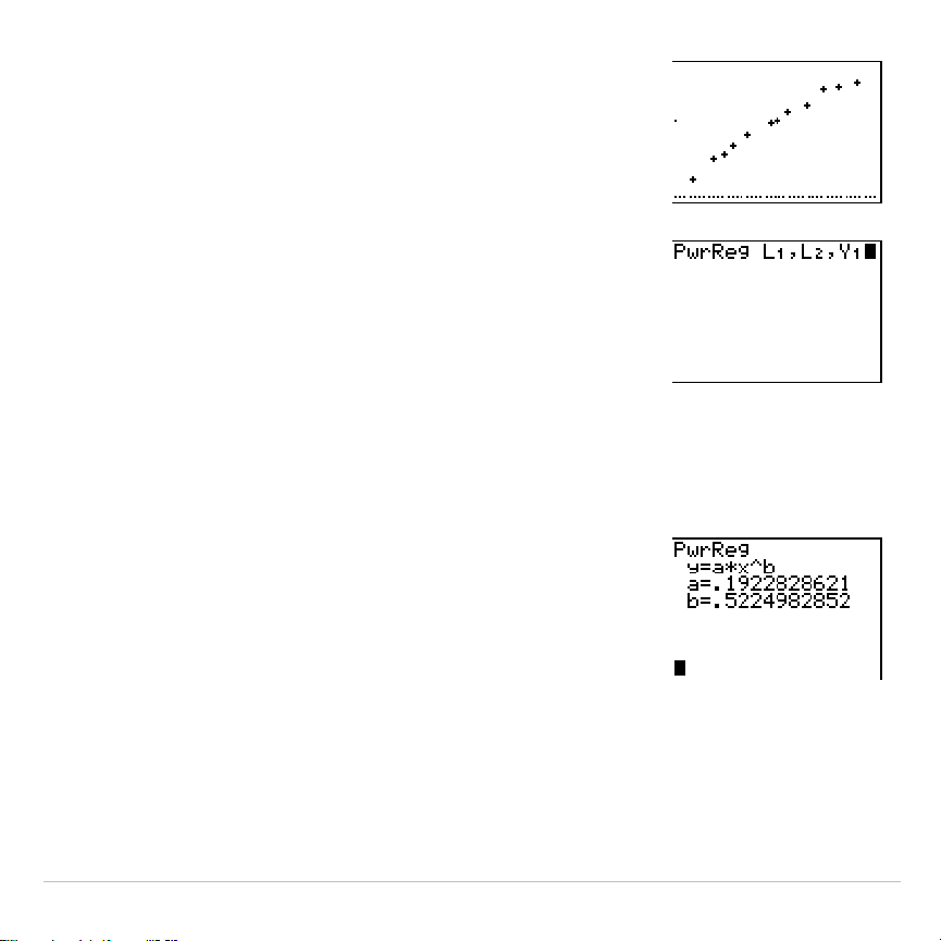
TI-83 Plus Statistics 323
23. Press
q
9
to select
9:ZoomStat
from the
ZOOM
menu. The window variables are
adjusted automatically, and the original scatter
plot of time-versus-length data (plot 1) is
displayed.
24. Press
…
~
ƒ
[
A
] to select
A:PwrReg
from the
STAT CALC
menu.
PwrReg
is pasted to
the home screen.
Press
y
d
¢
y
e
¢
. Press
~
1
to
display the
VARS Y
.
VARS FUNCTION
secondary
menu, and then press
1
to select
1:Y1
.
L1
,
L2
,
and
Y1
are pasted to the home screen as
arguments to
PwrReg
.
25. Press
Í
to calculate the power regression.
Values for
a
and
b
are displayed on the home
screen. The power regression equation is
stored in
Y1
. Residuals are calculated and
stored automatically in the list name
RESID
.
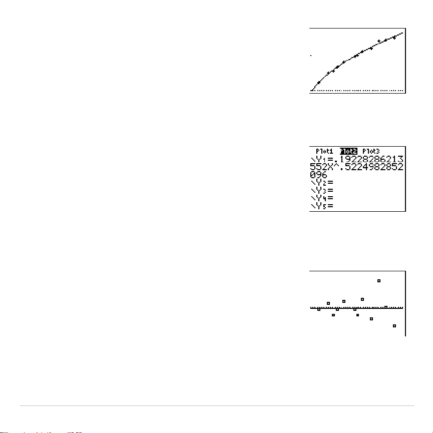
TI-83 Plus Statistics 324
26. Press
s
. The regression line and the
scatter plot are displayed.
The new function y=.192x
.
522
appears to fit the data well. To get more
information, examine a residual plot.
27. Press
o
to display the
Y=
editor.
Press
|
Í
to deselect
Y1
.
Press
}
Í
to turn off plot 1. Press
~
Í
to turn on plot 2.
Note: Step 19 defined plot 2 to plot residuals
(
RESID
) versus string length (
L1
).
28. Press
q
9
to select
9:ZoomStat
from the
ZOOM
menu. The window variables are
adjusted automatically, and plot 2 is displayed.
This is a scatter plot of the residuals.
The new residual plot shows that the residuals are random in sign, with
the residuals increasing in magnitude as the string length increases.
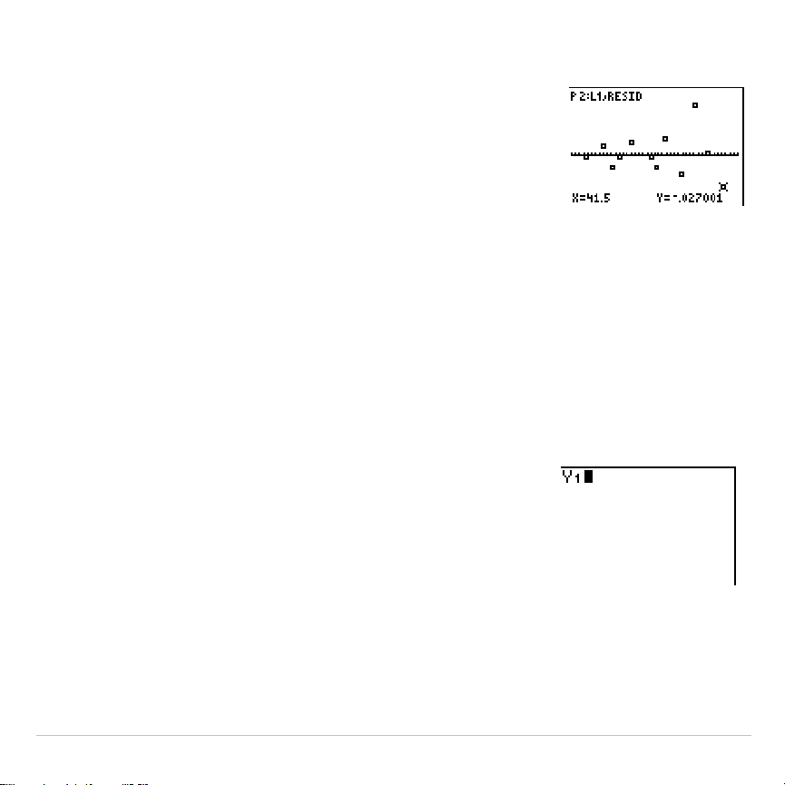
TI-83 Plus Statistics 325
To see the magnitudes of the residuals, continue with these steps.
29. Press
r
.
Press
~
and
|
to trace the data. Observe the
values for
Y
at each point.
With this model, the largest positive residual is
about 0.041 and the smallest negative residual
is about
L
0.027. All other residuals are less
than 0.02 in magnitude.
Now that you have a good model for the relationship between length and
period, you can use the model to predict the period for a given string
length. To predict the periods for a pendulum with string lengths of 20 cm
and 50 cm, continue with these steps.
30. Press
~
1
to display the
VARS Y
.
VARS
FUNCTION
secondary menu, and then press
1
to
select
1:Y1
.
Y1
is pasted to the home screen.
TI-83 Plus Statistics 326
31. Press
£
20
¤
to enter a string length of
20 cm.
Press
Í
to calculate the predicted time of
about 0.92 seconds.
Based on the residual analysis, we would
expect the prediction of about 0.92 seconds to
be within about 0.02 seconds of the actual
value.
TI-83 Plus Statistics 327
32. Press
y
[
to recall the Last Entry.
Press
|
|
|
5
to change the string length to
50 cm.
33. Press
Í
to calculate the predicted time of
about 1.48 seconds.
Since a string length of 50 cm exceeds the
lengths in the data set, and since residuals
appear to be increasing as string length
increases, we would expect more error with
this estimate.
Note: You also can make predictions using the
table with the
TABLE SETUP
settings
Indpnt:Ask
and
Depend:Auto
(Chapter 7).

TI-83 Plus Statistics 328
Setting Up Statistical Analyses
Using Lists to Store Data
Data for statistical analyses is stored in lists, which you can create and
edit using the stat list editor. The TI-83 Plus has six list variables in
memory,
L1
through
L6
, to which you can store data for statistical
calculations. Also, you can store data to list names that you create
(Chapter 11).
Setting Up a Statistical Analysis
To set up a statistical analysis, follow these steps. Read the chapter for
details.
1. Enter the statistical data into one or more lists.
2. Plot the data.
3. Calculate the statistical variables or fit a model to the data.
4. Graph the regression equation for the plotted data.
5. Graph the residuals list for the given regression model.
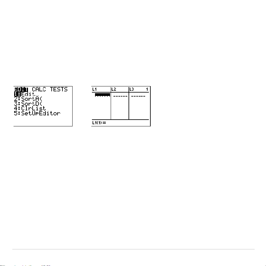
TI-83 Plus Statistics 329
Displaying the Stat List Editor
The stat list editor is a table where you can store, edit, and view up to 20
lists that are in memory. Also, you can create list names from the stat list
editor.
To display the stat list editor, press
…
, and then select
1:Edit
from the
STAT EDIT
menu.
The top line displays list names.
L1
through
L6
are stored in columns
1
through
6
after a memory reset. The number of the current column is
displayed in the top-right corner.
The bottom line is the entry line. All data entry occurs on this line. The
characteristics of this line change according to the current context.
The center area displays up to seven elements of up to three lists; it
abbreviates values when necessary. The entry line displays the full value
of the current element.

TI-83 Plus Statistics 330
Using the Stat List Editor
Entering a List Name in the Stat List Editor
To enter a list name in the stat list editor, follow these steps.
1. Display the
Name=
prompt in the entry line in either of two ways.
•
Move the cursor onto the list name in the column where you want
to insert a list, and then press
y
6
. An unnamed column is
displayed and the remaining lists shift right one column.
•
Press
}
until the cursor is on the top line, and then press
~
until
you reach the unnamed column.
Note: If list names are stored to all 20 columns, you must remove a list
name to make room for an unnamed column.
The
Name=
prompt is displayed and alpha-lock is on.
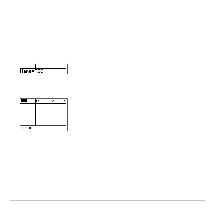
TI-83 Plus Statistics 331
2. Enter a valid list name in any of four ways.
•
Select a name from the
LIST NAMES
menu (Chapter 11).
•
Enter
L1
,
L2
,
L3
,
L4
,
L5
, or
L6
from the keyboard.
•
Enter an existing user-created list name directly from the keyboard.
•
Enter a new user-created list name.
3. Press
Í
or
†
to store the list name and its elements, if any, in
the current column of the stat list editor.
To begin entering, scrolling, or editing list elements, press
†
. The
rectangular cursor is displayed.
Note: If the list name you entered in step 2 already was stored in another stat
list editor column, then the list and its elements, if any, move to the current
column from the previous column. Remaining list names shift accordingly.

TI-83 Plus Statistics 332
Creating a Name in the Stat List Editor
To create a name in the stat list editor, follow these steps.
1. Display the
Name=
prompt.
2. Press [
letter from A to Z or
q
] to enter the first letter of the name. The
first character cannot be a number.
3. Enter zero to four letters,
q
, or numbers to complete the new user-
created list name. List names can be one to five characters long.
4. Press
Í
or
†
to store the list name in the current column of the
stat list editor. The list name becomes an item on the
LIST NAMES
menu (Chapter 11).
Removing a List from the Stat List Editor
To remove a list from the stat list editor, move the cursor onto the list
name and then press
{
. The list is not deleted from memory; it is only
removed from the stat list editor.
Note1: To delete a list name from memory, use the
MEMORY MANAGEMENT/
DELETE
secondary menu
(Chapter 18).
Note 2: If you archive a list, it will be removed from the stat list editor.

TI-83 Plus Statistics 333
Removing All Lists and Restoring L
1
through L
6
You can remove all user-created lists from the stat list editor and restore
list names
L1
through
L6
to columns
1
through
6
in either of two ways.
•
Use
SetUpEditor
with no arguments.
•
Reset all memory (Chapter 18).
Clearing All Elements from a List
You can clear all elements from a list in any of five ways.
•
Use
ClrList
to clear specified lists.
•
In the stat list editor, press
}
to move the cursor onto a list name,
and then press
‘
Í
.
•
In the stat list editor, move the cursor onto each element, and then
press
{
one by one.
•
On the home screen or in the program editor, enter
0
!
dim(
listname
)
to
set the dimension of
listname
to 0 (Chapter 11).
•
Use
ClrAllLists
to clear all lists in memory (Chapter 18).

TI-83 Plus Statistics 334
Editing a List Element
To edit a list element, follow these steps.
1. Move the rectangular cursor onto the element you want to edit.
2. Press
Í
to move the cursor to the entry line.
Note: If you want to replace the current value, you can enter a new value
without first pressing
Í
. When you enter the first character, the current
value is cleared automatically.
3. Edit the element in the entry line.
•
Press one or more keys to enter the new value. When you enter
the first character, the current value is cleared automatically.
•
Press
~
to move the cursor to the character before which you want
to insert, press
y
6
, and then enter one or more characters.
•
Press
~
to move the cursor to a character you want to delete, and
then press
{
to delete the character.
To cancel any editing and restore the original element at the
rectangular cursor, press
‘
Í
.
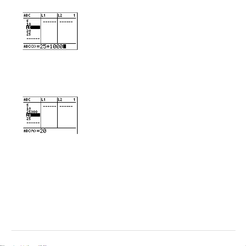
TI-83 Plus Statistics 335
Note:
You can enter expressions and variables for elements.
4. Press
Í
,
}
, or
†
to update the list. If you entered an expression,
it is evaluated. If you entered only a variable, the stored value is
displayed as a list element.
When you edit a list element in the stat list editor, the list is updated in
memory immediately.

TI-83 Plus Statistics 336
Attaching Formulas to List Names
Attaching a Formula to a List Name in Stat List Editor
You can attach a formula to a list name in the stat list editor, and then
display and edit the calculated list elements. When executed, the
attached formula must resolve to a list. Chapter 11 describes in detail the
concept of attaching formulas to list names.
To attach a formula to a list name that is stored in the stat list editor,
follow these steps.
1. Press
…
Í
to display the stat list editor.
2. Press
}
to move the cursor to the top line.
3. Press
|
or
~
, if necessary, to move the cursor onto the list name to
which you want to attach the formula.
Note: If a formula in quotation marks is displayed on the entry line, then a
formula is already attached to the list name. To edit the formula, press
Í
, and then edit the formula.
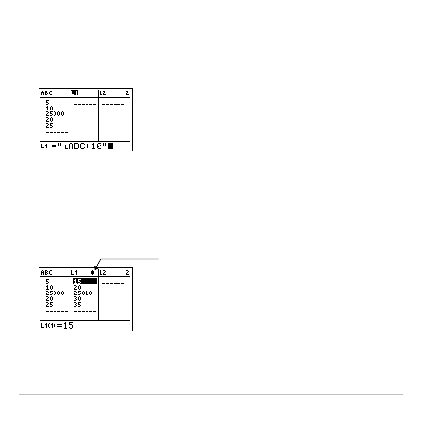
TI-83 Plus Statistics 337
4. Press
ƒ
[
ã
], enter the formula, and press
ƒ
[
ã
].
Note:
If you do not use quotation marks, the TI-83 Plus calculates and
displays the same initial list of answers, but does not attach the formula for
future calculations.
Note:
Any user-created list name referenced in a formula must be preceded
by an
Ù
symbol (Chapter 11).
5. Press
Í
. The TI-83 Plus calculates each list element and stores it
to the list name to which the formula is attached. A lock symbol is
displayed in the stat list editor, next to the list name to which the
formula is attached.
lock s
y
mbol
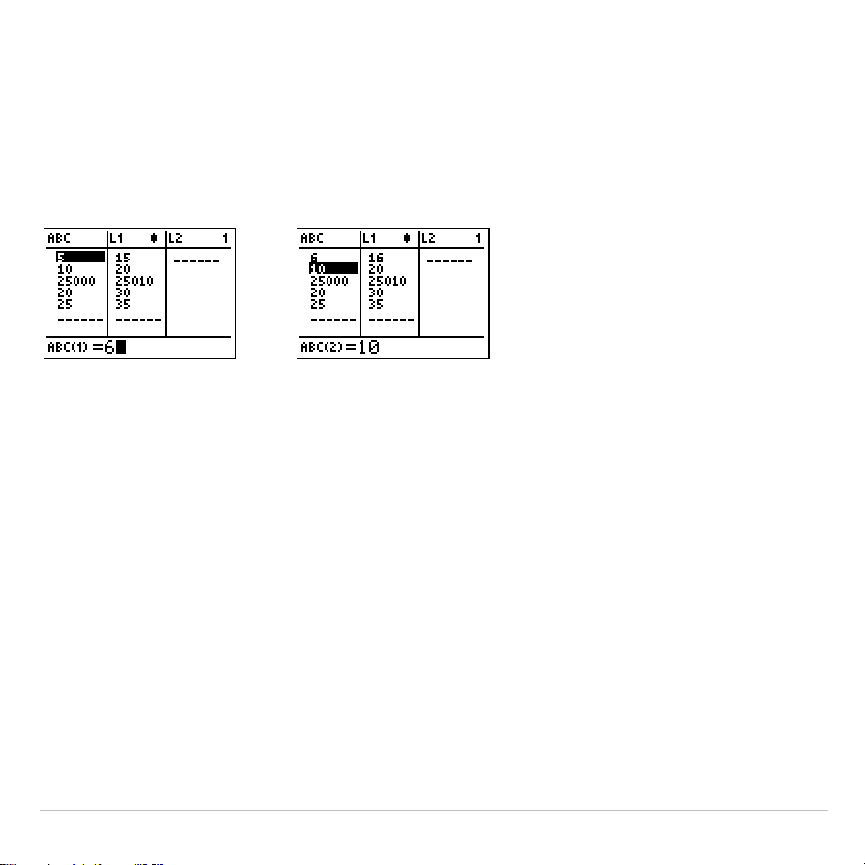
TI-83 Plus Statistics 338
Using the Stat List Editor When Formula-Generated Lists Are
Displayed
When you edit an element of a list referenced in an attached formula, the
TI-83 Plus updates the corresponding element in the list to which the
formula is attached (Chapter 11).
When a list with a formula attached is displayed in the stat list editor and
you edit or enter elements of another displayed list, then the TI-83 Plus
takes slightly longer to accept each edit or entry than when no lists with
formulas attached are in view.
Tip: To speed editing time, scroll horizontally until no lists with formulas are
displayed, or rearrange the stat list editor so that no lists with formulas are
displayed.

TI-83 Plus Statistics 339
Handling Errors Resulting from Attached Formulas
On the home screen, you can attach to a list a formula that references
another list with dimension 0 (Chapter 11). However, you cannot display
the formula-generated list in the stat list editor or on the home screen
until you enter at least one element to the list that the formula
references.
All elements of a list referenced by an attached formula must be valid for
the attached formula. For example, if
Real
number mode is set and the
attached formula is
log(L1)
, then each element of
L1
must be greater than
0, since the logarithm of a negative number returns a complex result.
Tip: If an error menu is returned when you attempt to display a formula-
generated list in the stat list editor, you can select
2:Goto
, write down the
formula that is attached to the list, and then press
‘
Í
to detach (clear)
the formula. You then can use the stat list editor to find the source of the error.
After making the appropriate changes, you can reattach the formula to a list.
If you do not want to clear the formula, you can select
1:Quit
, display the
referenced list on the home screen, and find and edit the source of the error. To
edit an element of a list on the home screen, store the new value to
listname
(
element#
)
(Chapter 11).

TI-83 Plus Statistics 340
Detaching Formulas from List Names
Detaching a Formula from a List Name
You can detach (clear) a formula from a list name in several ways.
For example:
•
In the stat list editor, move the cursor onto the name of the list to
which a formula is attached. Press
Í
‘
Í
. All list
elements remain, but the formula is detached and the lock symbol
disappears.
•
In the stat list editor, move the cursor onto an element of the list to
which a formula is attached. Press
Í
, edit the element, and then
press
Í
. The element changes, the formula is detached, and the
lock symbol disappears. All other list elements remain.
•
Use
ClrList
. All elements of one or more specified lists are cleared,
each formula is detached, and each lock symbol disappears. All list
names remain.
•
Use
ClrAllLists
(Chapter 18). All elements of all lists in memory are
cleared, all formulas are detached from all list names, and all lock
symbols disappear. All list names remain.

TI-83 Plus Statistics 341
Editing an Element of a Formula-Generated List
As described above, one way to detach a formula from a list name is to
edit an element of the list to which the formula is attached. The
TI-83 Plus protects against inadvertently detaching the formula from the
list name by editing an element of the formula-generated list.
Because of the protection feature, you must press
Í
before you can
edit an element of a formula-generated list.
The protection feature does not allow you to delete an element of a list to
which a formula is attached. To delete an element of a list to which a
formula is attached, you must first detach the formula in any of the ways
described above.
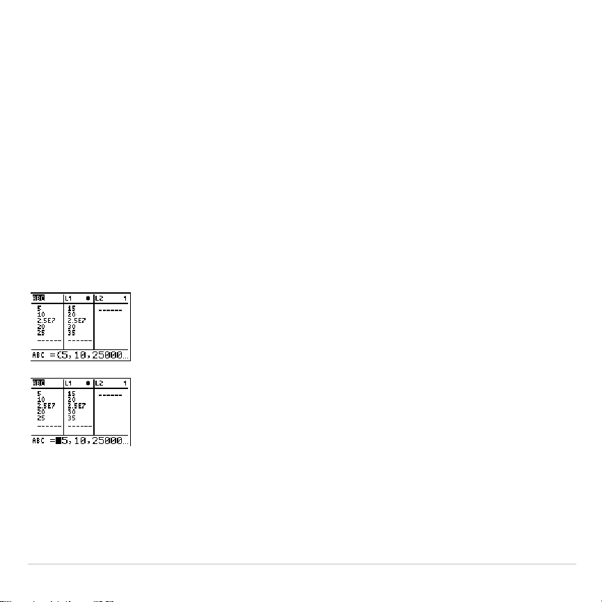
TI-83 Plus Statistics 342
Switching Stat List Editor Contexts
Stat List Editor Contexts
The stat list editor has four contexts.
•
View-elements context
•
Edit-elements context
•
View-names context
•
Enter-name context
The stat list editor is first displayed in view-elements context. To switch
through the four contexts, select
1:Edit
from the
STAT EDIT
menu and
follow these steps.
1. Press
}
to move the cursor onto a list name. You are
now in view-names context. Press
~
and
|
to view list
names stored in other stat list editor columns.
2. Press
Í
. You are now in edit-elements context.
You may edit any element in a list. All elements of the
current list are displayed in braces (
{
}
)in the entry
line. Press
~
and
|
to view more list elements.
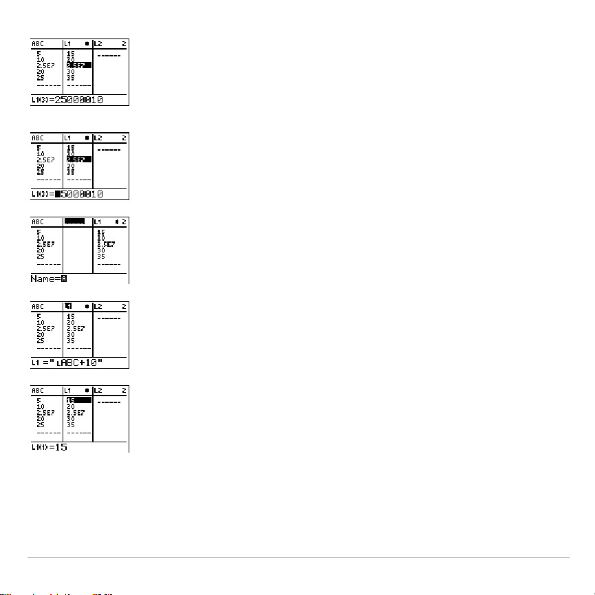
TI-83 Plus Statistics 343
3. Press
Í
again. You are now in view-elements
context. Press
~
,
|
,
†
, and
}
to view other list
elements. The current element’s full value is displayed
in the entry line.
4. Press
Í
again. You are now in edit-elements
context. You may edit the current element in the entry
line.
5. Press
}
until the cursor is on a list name, then press
y
6
. You are now in enter-name context.
6. Press
‘
. You are now in view-names context.
7. Press
†
. You are now back in view-elements context.
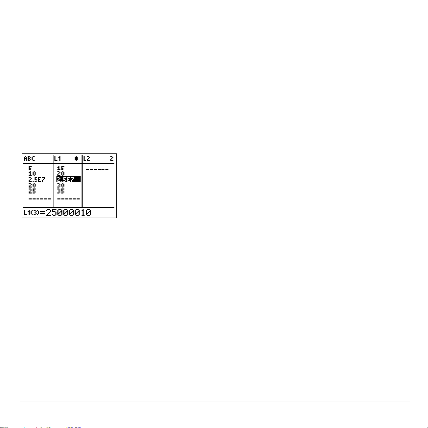
TI-83 Plus Statistics 344
Stat List Editor Contexts
View-Elements Context
In view-elements context, the entry line displays the list name, the
current element’s place in that list, and the full value of the current
element, up to 12 characters at a time. An ellipsis (
...
) indicates that the
element continues beyond 12 characters.
To page down the list six elements, press
ƒ
†
. To page up six
elements, press
ƒ
}
. To delete a list element, press
{
.
Remaining elements shift up one row. To insert a new element, press
y
6
.
0
is the default value for a new element.
Edit-Elements Context
In edit-elements context, the data displayed in the entry line depends on
the previous context.
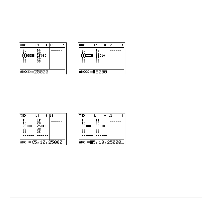
TI-83 Plus Statistics 345
•
When you switch to edit-elements context from view-elements
context, the full value of the current element is displayed. You can
edit the value of this element, and then press
†
and
}
to edit other
list elements.
&
•
When you switch to edit-elements context from view-names context,
the full values of all elements in the list are displayed. An ellipsis
indicates that list elements continue beyond the screen. You can
press
~
and
|
to edit any element in the list.
&
Note:
In edit-elements context, you can attach a formula to a list name only if
you switched to it from view-names context.
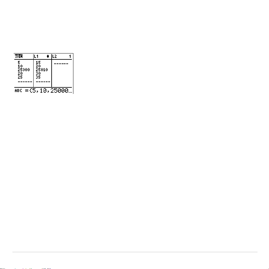
TI-83 Plus Statistics 346
View-Names Context
In view-names context, the entry line displays the list name and the list
elements.
To remove a list from the stat list editor, press
{
. Remaining lists shift
to the left one column. The list is not deleted from memory.
To insert a name in the current column, press
y
6
. Remaining
columns shift to the right one column.
Enter-Name Context
In enter-name context, the
Name=
prompt is displayed in the entry line,
and alpha-lock is on.
At the
Name=
prompt, you can create a new list name, paste a list name
from
L1
to
L6
from the keyboard, or paste an existing list name from the
LIST NAMES
menu (Chapter 11). The
Ù
symbol is not required at the
Name=
prompt.
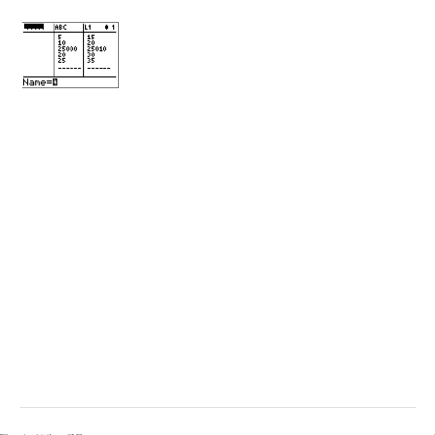
TI-83 Plus Statistics 347
To leave enter-name context without entering a list name, press
‘
.
The stat list editor switches to view-names context.
TI-83 Plus Statistics 348
STAT EDIT Menu
STAT EDIT Menu
To display the
STAT EDIT
menu, press
…
.
EDIT CALC TESTS
1:Edit
...
Displays the stat list editor.
2:SortA(
Sorts a list in ascending order.
3:SortD(
Sorts a list in descending order.
4:ClrList
Deletes all elements of a list.
5:SetUpEditor
Stores lists in the stat list editor.
Note: Chapter 13: Inferential Statistics describes the
STAT TESTS
menu items.
SortA(, SortD(
SortA(
(sort ascending) sorts list elements from low to high values.
SortD(
(sort descending) sorts list elements from high to low values. Complex
lists are sorted based on magnitude (modulus).
SortA(
and
SortD(
each
can sort in either of two ways.
•
With one
listname
,
SortA(
and
SortD(
sort the elements in
listname
and
update the list in memory.
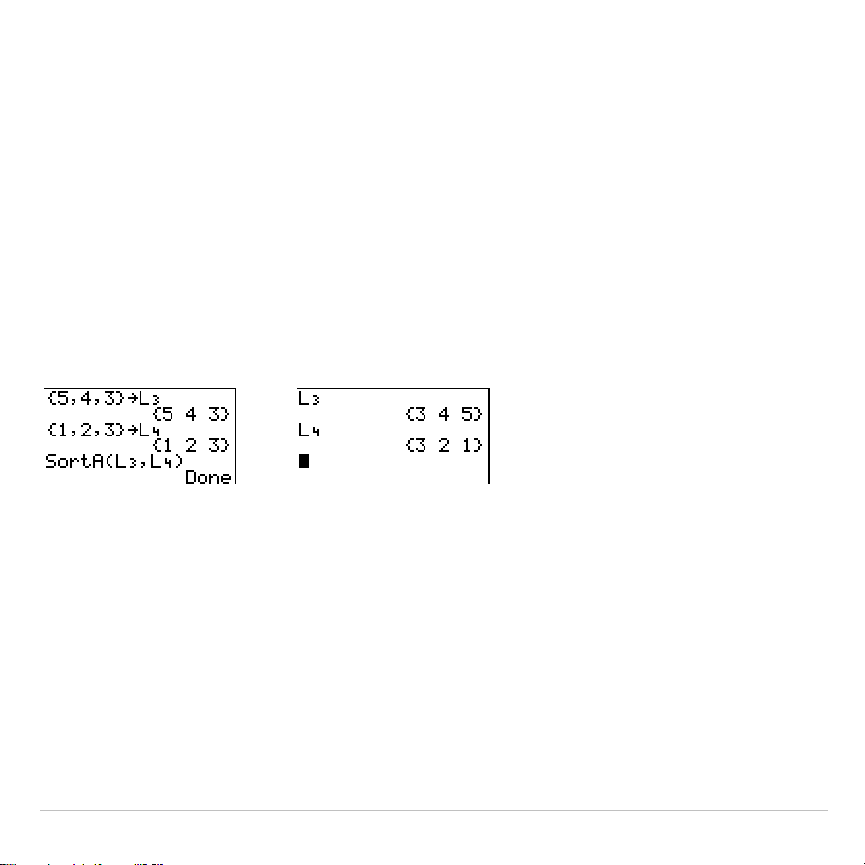
TI-83 Plus Statistics 349
•
With two or more lists,
SortA(
and
SortD(
sort
keylistname
, and then sort
each
dependlist
by placing its elements in the same order as the
corresponding elements in
keylistname
. This lets you sort two-variable
data on
X
and keep the data pairs together. All lists must have the
same dimension.
The sorted lists are updated in memory.
SortA(
listname
)
SortD(
listname
)
SortA(
keylistname
,
dependlist1
[
,
dependlist2
,
...
,
dependlist n
]
)
SortD(
keylistname
,
dependlist1
[
,
dependlist2
,
...
,
dependlist n
]
)
Note:
SortA(
and
SortD(
are the same as
SortA(
and
SortD(
on the
LIST OPS
menu.
ClrList
ClrList
clears (deletes) from memory the elements of one or more
listnames
.
ClrList
also detaches any formula attached to a
listname
.
ClrList
listname1
,
listname2
,
...
,
listname n
Note: To clear from memory all elements of all list names, use
ClrAllLists
(Chapter 18).
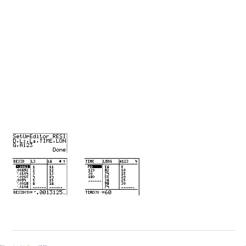
TI-83 Plus Statistics 350
SetUpEditor
With
SetUpEditor
you can set up the stat list editor to display one or more
listnames
in the order that you specify. You can specify zero to 20
listnames
.
Additionally, if you want to use
listnames
which happen to be archived, the
SetUp Editor will automatically unarchive the
listnames
and place them in
the stat list editor at the same time.
SetUpEditor
[
listname1
,
listname2
,
...
,
listname n
]
SetUpEditor
with one to 20
listnames
removes all list names from the stat
list editor and then stores
listnames
in the stat list editor columns in the
specified order, beginning in column
1
.
If you enter a
listname
that is not stored in memory already, then
listname
is
created and stored in memory; it becomes an item on the
LIST NAMES
menu.
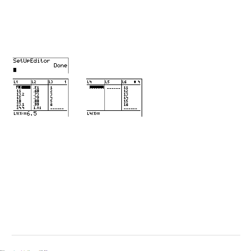
TI-83 Plus Statistics 351
Restoring L
1
through L
6
to the Stat List Editor
SetUpEditor
with no
listnames
removes all list names from the stat list
editor and restores list names
L1
through
L6
in the stat list editor columns
1
through
6
.

TI-83 Plus Statistics 352
Regression Model Features
Regression Model Features
STAT CALC
menu items
3
through
C
are regression models. The automatic
residual list and automatic regression equation features apply to all
regression models. Diagnostics display mode applies to some regression
models.
Automatic Residual List
When you execute a regression model, the automatic residual list feature
computes and stores the residuals to the list name
RESID
.
RESID
becomes an item on the
LIST NAMES
menu (Chapter 11).
The TI-83 Plus uses the formula below to compute
RESID
list elements.
The next section describes the variable
RegEQ
.
RESID
=
Ylistname
N
RegEQ
(
Xlistname
)
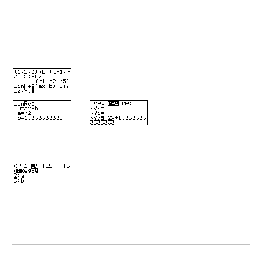
TI-83 Plus Statistics 353
Automatic Regression Equation
Each regression model has an optional argument,
regequ
, for which you
can specify a
Y=
variable such as
Y1
. Upon execution, the regression
equation is stored automatically to the specified
Y=
variable and the
Y=
function is selected.
Regardless of whether you specify a
Y=
variable for
regequ
, the
regression equation always is stored to the TI-83 Plus variable
RegEQ
,
which is item
1
on the
VARS Statistics EQ
secondary menu.
Note: For the regression equation, you can use the fixed-decimal mode setting
to control the number of digits stored after the decimal point (Chapter 1).
However, limiting the number of digits to a small number could affect the
accuracy of the fit.
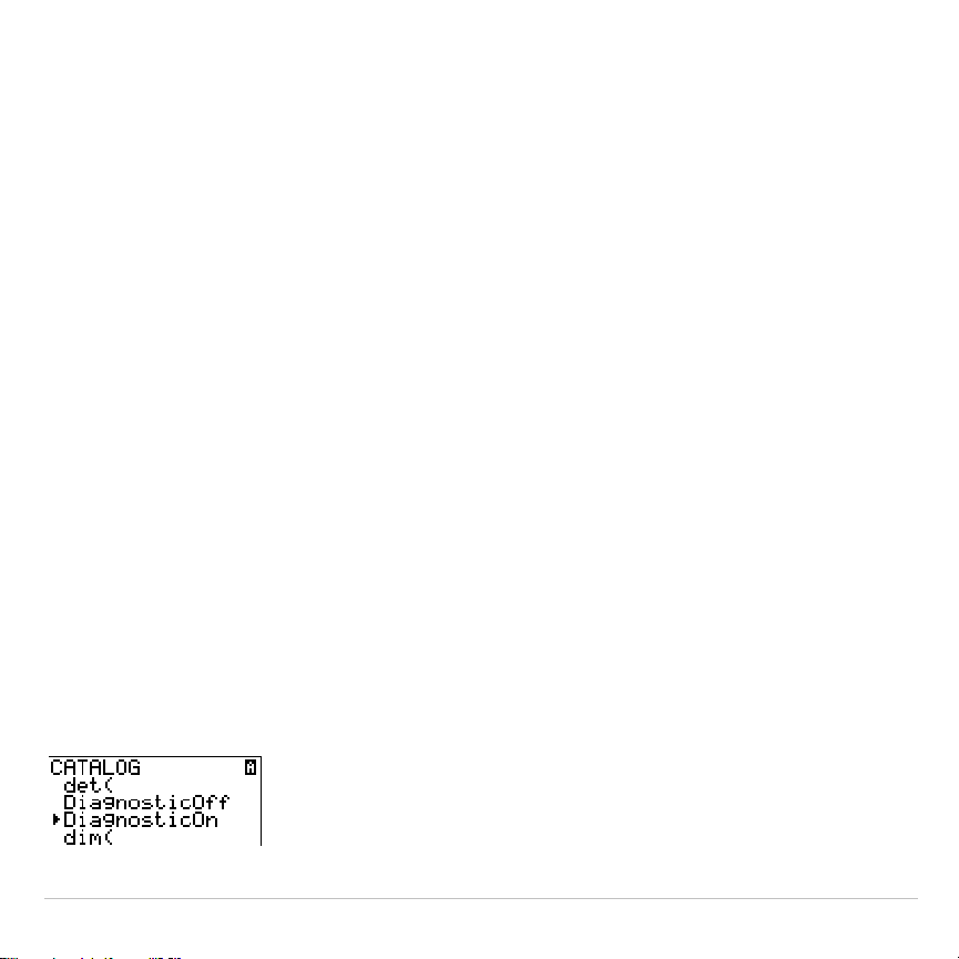
TI-83 Plus Statistics 354
Diagnostics Display Mode
When you execute some regression models, the TI-83 Plus computes
and stores diagnostics values for
r
(correlation coefficient) and
r
2
(coefficient of determination) or for
R
2
(coefficient of determination).
r
and
r
2
are computed and stored for these regression models.
LinReg(ax+b) LnReg PwrReg
LinReg(a+bx) ExpReg
R
2
is computed and stored for these regression models.
QuadReg CubicReg QuartReg
The
r
and
r
2
that are computed for
LnReg
,
ExpReg
, and
PwrReg
are
based on the linearly transformed data. For example, for
ExpReg
(y=ab^x),
r
and
r
2
are computed on ln y=ln a+x(ln b).
By default, these values are not displayed with the results of a
regression model when you execute it. However, you can set the
diagnostics display mode by executing the
DiagnosticOn
or
DiagnosticOff
instruction. Each instruction is in the
CATALOG
(Chapter 15).
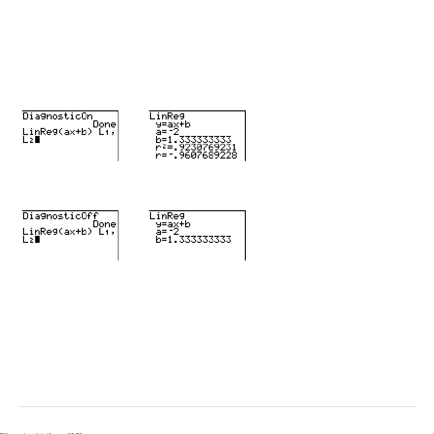
TI-83 Plus Statistics 355
Note:
To set
DiagnosticOn
or
DiagnosticOff
from the home screen, press
y
N
, and then select the instruction for the mode you want. The instruction
is pasted to the home screen. Press
Í
to set the mode.
When
DiagnosticOn
is set, diagnostics are displayed with the results
when you execute a regression model.
When
DiagnosticOff
is set, diagnostics are not displayed with the results
when you execute a regression model.
TI-83 Plus Statistics 356
STAT CALC Menu
STAT CALC Menu
To display the
STAT CALC
menu, press
…
~
.
EDIT CALC TESTS
1:1-Var Stats
Calculates 1-variable statistics.
2:2-Var Stats
Calculates 2-variable statistics.
3:Med-Med
Calculates a median-median line.
4:LinReg(ax+b)
Fits a linear model to data.
5:QuadReg
Fits a quadratic model to data.
6:CubicReg
Fits a cubic model to data.
7:QuartReg
Fits a quartic model to data.
8:LinReg(a+bx)
Fits a linear model to data.
9:LnReg
Fits a logarithmic model to data.
0:ExpReg
Fits an exponential model to data.
A:PwrReg
Fits a power model to data.
B:Logistic
Fits a logistic model to data.
C:SinReg
Fits a sinusoidal model to data.
For each
STAT CALC
menu item, if neither
Xlistname
nor
Ylistname
is
specified, then the default list names are
L1
and
L2
. If you do not specify
freqlist
, then the default is
1
occurrence of each list element.

TI-83 Plus Statistics 357
Frequency of Occurrence for Data Points
For most
STAT CALC
menu items, you can specify a list of data
occurrences, or frequencies (
freqlist
).
Each element in
freqlist
indicates how many times the corresponding data
point or data pair occurs in the data set you are analyzing.
For example, if
L1={15,12,9,14}
and
Ù
FREQ={1,4,1,3}
, then the TI-83 Plus
interprets the instruction
1
.
Var Stats
L1
,
Ù
FREQ
to mean that
15
occurs
once,
12
occurs four times,
9
occurs once, and
14
occurs three times.
Each element in
freqlist
must be
‚
0, and at least one element must be > 0.
Noninteger
freqlist
elements are valid. This is useful when entering
frequencies expressed as percentages or parts that add up to 1.
However, if
freqlist
contains noninteger frequencies,
Sx
and
Sy
are
undefined; values are not displayed for
Sx
and
Sy
in the statistical
results.
1
.
Var Stats
1
.
Var Stats
(one-variable statistics) analyzes data with one measured
variable. Each element in
freqlist
is the frequency of occurrence for each
corresponding data point in
Xlistname
.
freqlist
elements must be real
numbers > 0.
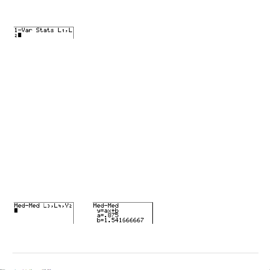
TI-83 Plus Statistics 358
1
.
Var Stats
[
Xlistname
,
freqlist
]
2
.
Var Stats
2
.
Var Stats
(two-variable statistics) analyzes paired data.
Xlistname
is the
independent variable.
Ylistname
is the dependent variable. Each element
in
freqlist
is the frequency of occurrence for each data pair
(
Xlistname,Ylistname
).
2
.
Var Stats
[
Xlistname
,
Ylistname
,
freqlist
]
Med
.
Med (ax+b)
Med
.
Med
(median-median) fits the model equation y=ax+b to the data
using the median-median line (resistant line) technique, calculating the
summary points
x
1
,
y
1
,
x
2
,
y
2
,
x
3
, and
y
3
.
Med
.
Med
displays values for
a
(slope) and
b
(y-intercept).
Med
.
Med
[
Xlistname
,
Ylistname
,
freqlist
,
regequ
]

TI-83 Plus Statistics 359
LinReg (ax+b)
LinReg(ax+b)
(linear regression) fits the model equation y=ax+b to the data
using a least-squares fit. It displays values for
a
(slope) and
b
(y-intercept);
when
DiagnosticOn
is set, it also displays values for
r
2
and
r
.
LinReg(ax+b)
[
Xlistname
,
Ylistname
,
freqlist
,
regequ
]
QuadReg (ax
2
+bx+c)
QuadReg
(quadratic regression) fits the second-degree polynomial
y=ax
2
+bx+c to the data. It displays values for
a
,
b
, and
c
; when
DiagnosticOn
is set, it also displays a value for
R
2
. For three data points,
the equation is a polynomial fit; for four or more, it is a polynomial
regression. At least three data points are required.
QuadReg
[
Xlistname
,
Ylistname
,
freqlist
,
regequ
]
CubicReg—(ax
3
+bx
2
+cx+d)
CubicReg
(cubic regression) fits the third-degree polynomial
y=ax
3
+bx
2
+cx+d to the data. It displays values for
a
,
b
,
c
, and
d
; when
DiagnosticOn
is set, it also displays a value for
R
2
. For four points, the
equation is a polynomial fit; for five or more, it is a polynomial regression.
At least four points are required.

TI-83 Plus Statistics 360
CubicReg
[
Xlistname
,
Ylistname
,
freqlist
,
regequ
]
QuartReg—(ax
4
+bx
3
+cx
2
+ dx+e)
QuartReg
(quartic regression) fits the fourth-degree polynomial
y=ax
4
+bx
3
+cx
2
+dx+e to the data. It displays values for
a
,
b
,
c
,
d
, and
e
;
when
DiagnosticOn
is set, it also displays a value for
R
2
. For five points,
the equation is a polynomial fit; for six or more, it is a polynomial
regression. At least five points are required.
QuartReg
[
Xlistname
,
Ylistname
,
freqlist
,
regequ
]
LinReg—(a+bx)
LinReg(a+bx)
(linear regression) fits the model equation y=a+bx to the data
using a least-squares fit. It displays values for
a
(y-intercept) and
b
(slope);
when
DiagnosticOn
is set, it also displays values for
r
2
and
r
.
LinReg(a+bx)
[
Xlistname
,
Ylistname
,
freqlist
,
regequ
]
LnReg—(a+b ln(x))
LnReg
(logarithmic regression) fits the model equation y=a+b ln(x) to the
data using a least-squares fit and transformed values ln(x) and y. It
displays values for
a
and
b
; when
DiagnosticOn
is set, it also displays
values for
r
2
and
r
.

TI-83 Plus Statistics 361
LnReg
[
Xlistname
,
Ylistname
,
freqlist
,
regequ
]
ExpReg—(ab
x
)
ExpReg
(exponential regression) fits the model equation y=ab
x
to the data
using a least-squares fit and transformed values x and ln(y). It displays
values for
a
and
b
; when
DiagnosticOn
is set, it also displays values for
r
2
and
r
.
ExpReg
[
Xlistname
,
Ylistname
,
freqlist
,
regequ
]
PwrReg—(ax
b
)
PwrReg
(power regression) fits the model equation y=ax
b
to the data using
a least-squares fit and transformed values ln(x) and ln(y). It displays
values for
a
and
b
; when
DiagnosticOn
is set, it also displays values for
r
2
and
r
.
PwrReg
[
Xlistname
,
Ylistname
,
freqlist
,
regequ
]
Logistic—c/(1+a
ä
e
L
bx
)
Logistic
fits the model equation y=c/(1+a
ä
e
L
bx
) to the data using an
iterative least-squares fit. It displays values for
a
,
b
, and
c
.
Logistic
[
Xlistname
,
Ylistname
,
freqlist
,
regequ
]

TI-83 Plus Statistics 362
SinReg—a sin(bx+c)+d
SinReg
(sinusoidal regression) fits the model equation y=a sin(bx+c)+d to
the data using an iterative least-squares fit. It displays values for
a
,
b
,
c
,
and
d
. At least four data points are required. At least two data points per
cycle are required in order to avoid aliased frequency estimates.
SinReg
[
iterations
,
Xlistname
,
Ylistname
,
period
,
regequ
]
iterations
is the maximum number of times the algorithm will iterate to find
a solution. The value for
iterations
can be an integer
‚
1 and
16; if not
specified, the default is 3. The algorithm may find a solution before
iterations
is reached. Typically, larger values for
iterations
result in longer
execution times and better accuracy for
SinReg
, and vice versa.
A
period
guess is optional. If you do not specify
period
, the difference
between time values in
Xlistname
must be equal and the time values must
be ordered in ascending sequential order. If you specify
period
, the
algorithm may find a solution more quickly, or it may find a solution when
it would not have found one if you had omitted a value for
period
. If you
specify
period
, the differences between time values in
Xlistname
can be
unequal.
Note: The output of
SinReg
is always in radians, regardless of the
Radian/Degree
mode setting.
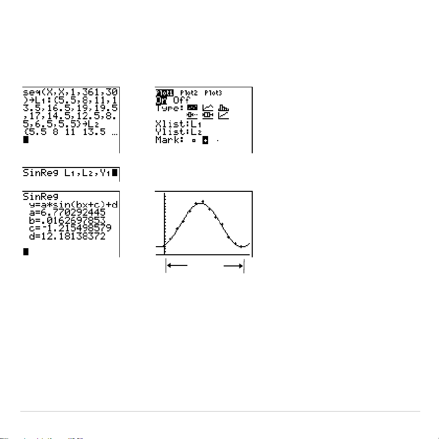
TI-83 Plus Statistics 363
SinReg Example: Daylight Hours in Alaska for One Year
Compute the regression model for the number of hours of daylight in
Alaska during one year.
&
&
With noisy data, you will achieve better convergence results when you
specify an accurate estimate for
period
. You can obtain a
period
guess in
either of two ways.
•
Plot the data and trace to determine the x-distance between the
beginning and end of one complete period, or cycle. The illustration
above and to the right graphically depicts a complete period, or cycle.
1 period

TI-83 Plus Statistics 364
•
Plot the data and trace to determine the x-distance between the
beginning and end of N complete periods, or cycles. Then divide the
total distance by N.
After your first attempt to use
SinReg
and the default value for
iterations
to
fit the data, you may find the fit to be approximately correct, but not
optimal. For an optimal fit, execute
SinReg 16,
Xlistname
,
Ylistname
,2
p
/
b
where
b
is the value obtained from the previous
SinReg
execution.

TI-83 Plus Statistics 365
Statistical Variables
The statistical variables are calculated and stored as indicated below. To
access these variables for use in expressions, press
, and select
5:Statistics
. Then select the
VARS
menu shown in the column below under
VARS
menu. If you edit a list or change the type of analysis, all statistical
variables are cleared.
Variables
1
.
Var
Stats
2
.
Var
Stats Other
VARS
menu
mean of
x
values
vv
XY
sum of
x
values
G
x
G
x
G
sum of
x
2
values
G
x
2
G
x
2
G
sample standard deviation of
xSxSx XY
population standard deviation of
x
s
x
s
x XY
number of data points
nn XY
mean of
y
values
w
XY
sum of
y
values
G
y
G
sum of
y
2
values
G
y
2
G
sample standard deviation of
ySyXY
population standard deviation of
y
s
y XY
sum of
x
…
y
G
xy
G
minimum of
x
values
minX minX XY

TI-83 Plus Statistics 366
Variables
1
.
Var
Stats
2
.
Var
Stats Other
VARS
menu
maximum of
x
values
maxX maxX XY
minimum of
y
values
minY XY
maximum of
y
values
maxY XY
1st quartile
Q1 PTS
median
Med PTS
3rd quartile
Q3 PTS
regression/fit coefficients
a
,
b EQ
polynomial,
Logistic
, and
SinReg
coefficients
a
,
b
,
c
,
d
,
e
EQ
correlation coefficient
r EQ
coefficient of determination
r
2
,
R
2
EQ
regression equation
RegEQ EQ
summary points (
Med
.
Med
only)
x1
,
y1
,
x2
,
y2
,
x3
,
y3
PTS
Q
1
and Q
3
The first quartile (
Q1
) is the median of points between
minX
and
Med
(median). The third quartile (
Q3
) is the median of points between
Med
and
maxX
.
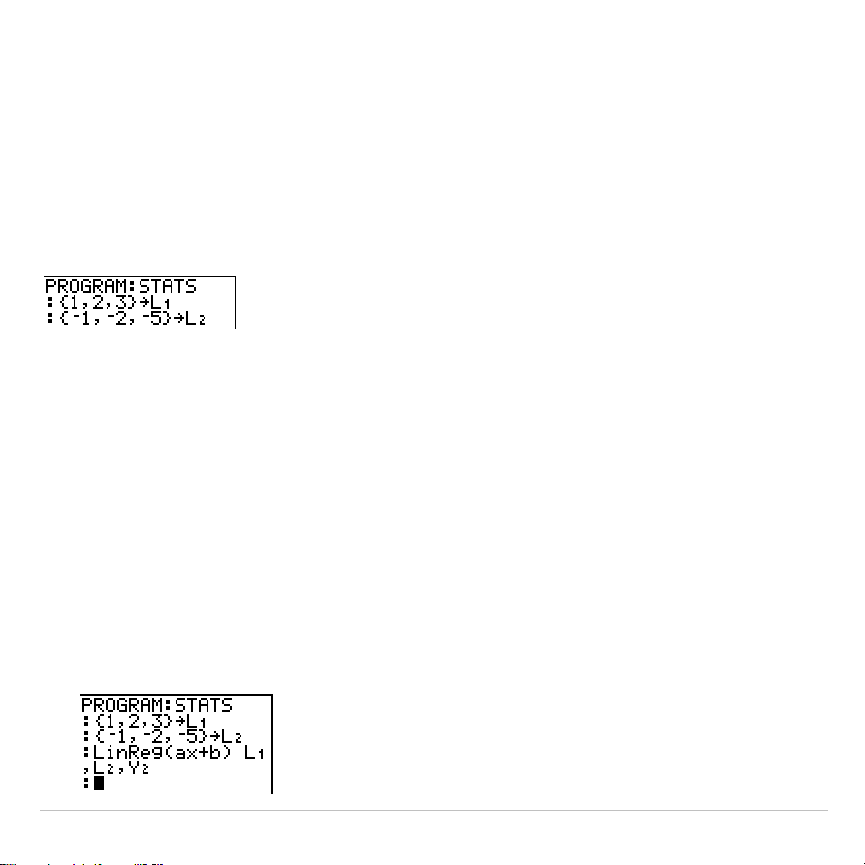
TI-83 Plus Statistics 367
Statistical Analysis in a Program
Entering Stat Data
You can enter statistical data, calculate statistical results, and fit models
to data from a program. You can enter statistical data into lists directly
within the program (Chapter 11).
Statistical Calculations
To perform a statistical calculation from a program, follow these steps.
1. On a blank line in the program editor, select the type of calculation
from the
STAT CALC
menu.
2. Enter the names of the lists to use in the calculation. Separate the list
names with a comma.
3. Enter a comma and then the name of a
Y=
variable, if you want to store
the regression equation to a
Y=
variable.

TI-83 Plus Statistics 368
Statistical Plotting
Steps for Plotting Statistical Data in Lists
You can plot statistical data that is stored in lists. The six types of plots
available are scatter plot, xyLine, histogram, modified box plot, regular
box plot, and normal probability plot. You can define up to three plots.
To plot statistical data in lists, follow these steps.
1. Store the stat data in one or more lists.
2. Select or deselect
Y=
functions as appropriate.
3. Define the stat plot.
4. Turn on the plots you want to display.
5. Define the viewing window.
6. Display and explore the graph.
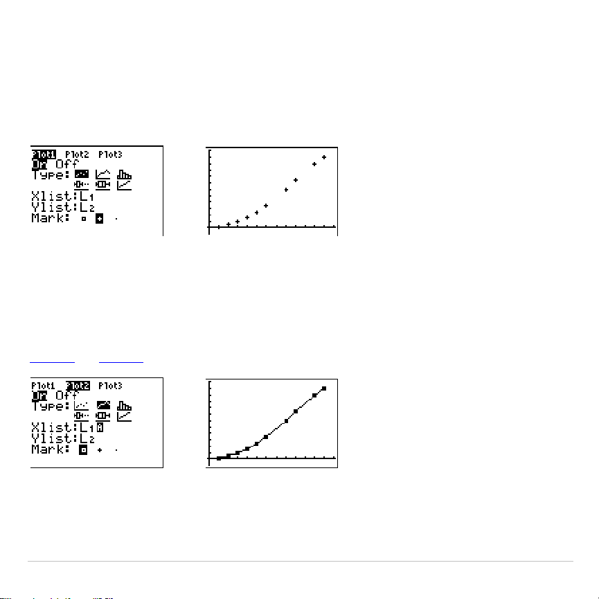
TI-83 Plus Statistics 369
"
(Scatter)
Scatter
plots plot the data points from
Xlist
and
Ylist
as coordinate pairs,
showing each point as a box (
›
), cross (
+
), or dot (
¦
).
Xlist
and
Ylist
must be the same length. You can use the same list for
Xlist
and
Ylist
.
Ó
(xyLine)
xyLine
is a scatter plot in which the data points are plotted and
connected in order of appearance in
Xlist
and
Ylist
. You may want to use
SortA(
or
SortD(
to sort the lists before you plot them.

TI-83 Plus Statistics 370
Ò
(Histogram)
Histogram
plots one-variable data. The
Xscl
window variable value
determines the width of each bar, beginning at
Xmin
.
ZoomStat
adjusts
Xmin
,
Xmax
,
Ymin
, and
Ymax
to include all values, and also adjusts
Xscl
.
The inequality (
Xmax
N
Xmin
)
à
Xscl
47 must be true. A value that occurs
on the edge of a bar is counted in the bar to the right.
Õ
(ModBoxplot)
ModBoxplot
(modified box plot) plots one-variable data, like the regular
box plot, except points that are 1.5
ä
Interquartile Range beyond the
quartiles. (The Interquartile Range is defined as the difference between
the third quartile
Q
3
and the first quartile
Q
1
.) These points are plotted
individually beyond the whisker, using the
Mark
(
›
or
+
or
¦
) you select.
You can trace these points, which are called outliers.
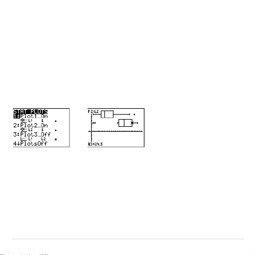
TI-83 Plus Statistics 371
The prompt for outlier points is
x=
, except when the outlier is the
maximum point (
maxX
) or the minimum point (
minX
). When outliers exist,
the end of each whisker will display
x=
. When no outliers exist,
minX
and
maxX
are the prompts for the end of each whisker.
Q1
,
Med
(median), and
Q3
define the box.
Box plots are plotted with respect to
Xmin
and
Xmax
, but ignore
Ymin
and
Ymax
. When two box plots are plotted, the first one plots at the top of the
screen and the second plots in the middle. When three are plotted, the
first one plots at the top, the second in the middle, and the third at the
bottom.
Ö
(Boxplot)
Boxplot
(regular box plot) plots one-variable data. The whiskers on the
plot extend from the minimum data point in the set (
minX
) to the first
quartile (
Q1
) and from the third quartile (
Q3
) to the maximum point
(
maxX
). The box is defined by
Q1
,
Med
(median), and
Q3
.
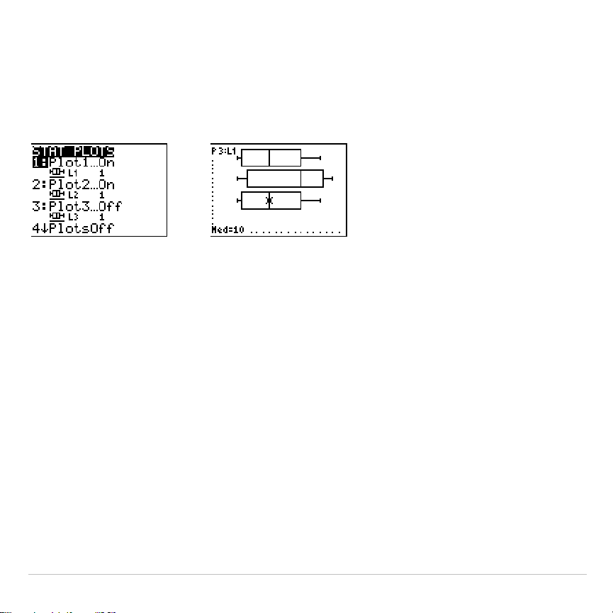
TI-83 Plus Statistics 372
Box plots are plotted with respect to
Xmin
and
Xmax
, but ignore
Ymin
and
Ymax
. When two box plots are plotted, the first one plots at the top of the
screen and the second plots in the middle. When three are plotted, the
first one plots at the top, the second in the middle, and the third at the
bottom.
Ô
(NormProbPlot)
NormProbPlot
(normal probability plot) plots each observation
X
in
Data List
versus the corresponding quantile
z
of the standard normal
distribution. If the plotted points lie close to a straight line, then the plot
indicates that the data are normal.
Enter a valid list name in the
Data List
field. Select
X
or
Y
for the
Data Axis
setting.
•
If you select
X
, the TI-83 Plus plots the data on the x-axis and the
z-values on the y-axis.
•
If you select
Y
, the TI-83 Plus plots the data on the y-axis and the
z-values on the x-axis.
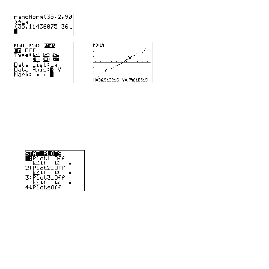
TI-83 Plus Statistics 373
Defining the Plots
To define a plot, follow these steps.
1. Press
y
,
. The
STAT PLOTS
menu is displayed with the
current plot definitions.
2. Select the plot you want to use. The stat plot editor is displayed for
the plot you selected.
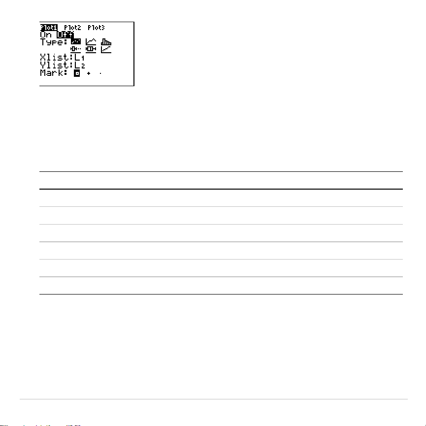
TI-83 Plus Statistics 374
3. Press
Í
to select
On
if you want to plot the statistical data
immediately. The definition is stored whether you select
On
or
Off
.
4. Select the type of plot. Each type prompts for the options checked in
this table.
Plot Type
XList YList Mark Freq
Data List Data Axis
"
Scatter
œœ œ
Ó
œœ œ
Ò
œœœ œ
Õ
œœ œ
Ö
œœœ œ
Ô
œœœ
5. Enter list names or select options for the plot type.
•
Xlist
(list name containing independent data)
•
Ylist
(list name containing dependent data)
•
Mark
(
›
or
+
or
¦
)
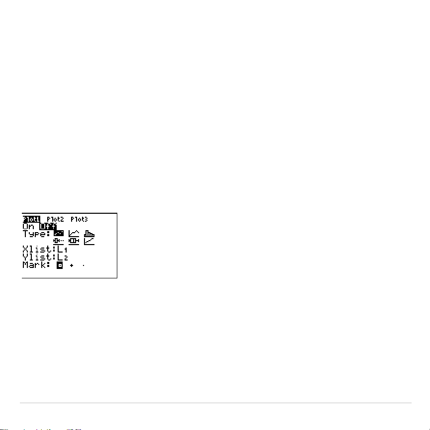
TI-83 Plus Statistics 375
•
Freq
(frequency list for
Xlist
elements; default is
1
)
•
Data List
(list name for
NormProbPlot
)
•
Data Axis
(axis on which to plot
Data List
)
Displaying Other Stat Plot Editors
Each stat plot has a unique stat plot editor. The name of the current stat
plot (
Plot1
,
Plot2
, or
Plot3
) is highlighted in the top line of the stat plot
editor. To display the stat plot editor for a different plot, press
}
,
~
, and
|
to move the cursor onto the name in the top line, and then press
Í
. The stat plot editor for the selected plot is displayed, and the
selected name remains highlighted.
Turning On and Turning Off Stat Plots
PlotsOn
and
PlotsOff
allow you to turn on or turn off stat plots from the
home screen or a program. With no plot number,
PlotsOn
turns on all
plots and
PlotsOff
turns off all plots. With one or more plot numbers (
1
,
2
,
and
3
),
PlotsOn
turns on specified plots, and
PlotsOff
turns off specified
plots.
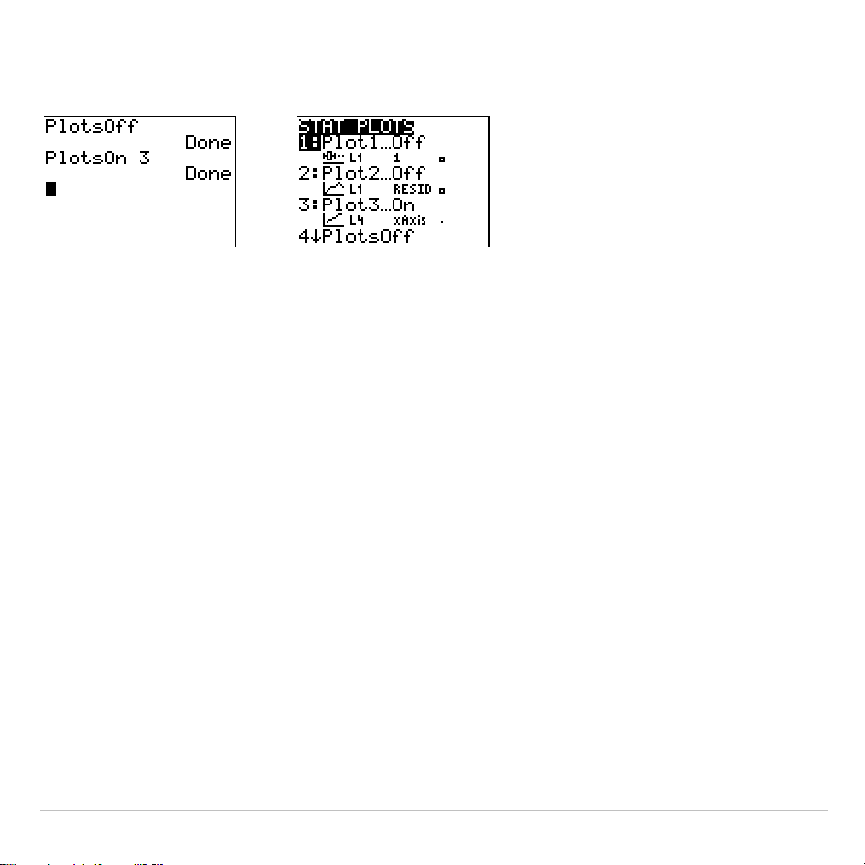
TI-83 Plus Statistics 376
PlotsOff
[
1,2,3
]
PlotsOn
[
1,2,3
]
Note: You also can turn on and turn off stat plots in the top line of the Y= editor
(Chapter 3).
Defining the Viewing Window
Stat plots are displayed on the current graph. To define the viewing
window, press
p
and enter values for the window variables.
ZoomStat
redefines the viewing window to display all statistical data
points.
Tracing a Stat Plot
When you trace a scatter plot or xyLine, tracing begins at the first
element in the lists.
When you trace a histogram, the cursor moves from the top center of
one column to the top center of the next, starting at the first column.

TI-83 Plus Statistics 377
When you trace a box plot, tracing begins at
Med
(the median). Press
|
to trace to
Q1
and
minX
. Press
~
to trace to
Q3
and
maxX
.
When you press
}
or
†
to move to another plot or to another Y=
function, tracing moves to the current or beginning point on that plot (not
the nearest pixel).
The
ExprOn
/
ExprOff
format setting applies to stat plots (Chapter 3). When
ExprOn
is selected, the plot number and plotted data lists are displayed
in the top-left corner.
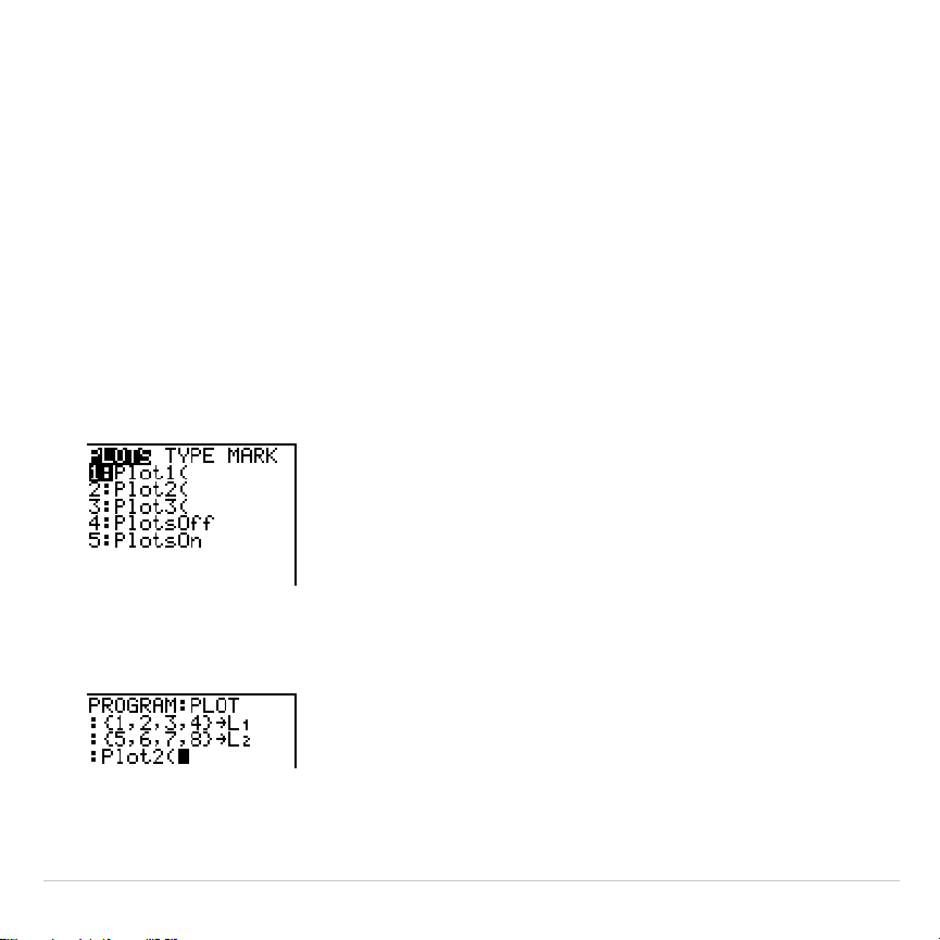
TI-83 Plus Statistics 378
Statistical Plotting in a Program
Defining a Stat Plot in a Program
To display a stat plot from a program, define the plot, and then display
the graph.
To define a stat plot from a program, begin on a blank line in the
program editor and enter data into one or more lists; then, follow these
steps.
1. Press
y
,
to display the
STAT PLOTS
menu.
2. Select the plot to define, which pastes
Plot1(
,
Plot2(
, or
Plot3(
to the
cursor location.
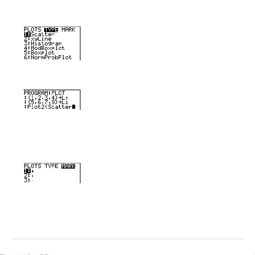
TI-83 Plus Statistics 379
3. Press
y
,
~
to display the
STAT TYPE
menu.
4. Select the type of plot, which pastes the name of the plot type to the
cursor location.
5. Press
¢
. Enter the list names, separated by commas.
6. Press
¢
y
,
|
to display the
STAT PLOT MARK
menu. (This
step is not necessary if you selected
3:Histogram
or
5:Boxplot
in
step 4.)
Select the type of mark (
›
or
+
or
¦
) for each data point. The selected
mark symbol is pasted to the cursor location.
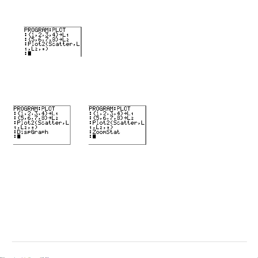
TI-83 Plus Statistics 380
7. Press
¤
Í
to complete the command line.
Displaying a Stat Plot from a Program
To display a plot from a program, use the
DispGraph
instruction
(Chapter 16) or any of the
ZOOM
instructions (Chapter 3).

TI-83 Plus Inferential Statistics and Distributions 381
Chapter 13:
Inferential Statistics and Distributions
Getting Started: Mean Height of a
Population
Getting Started is a fast-paced introduction. Read the chapter for details.
Suppose you want to estimate the mean height of a population of women given
the random sample below. Because heights among a biological population tend
to be normally distributed, a
t
distribution confidence interval can be used when
estimating the mean. The 10 height values below are the first 10 of 90 values,
randomly generated from a normally distributed population with an assumed
mean of 165.1 centimeters and a standard deviation of 6.35 centimeters
(
randNorm(165.1,6.35,90
) with a seed of 789).
Height (in centimeters) of Each of 10 Women
169.43 168.33 159.55 169.97 159.79 181.42 171.17 162.04
167.15 159.53
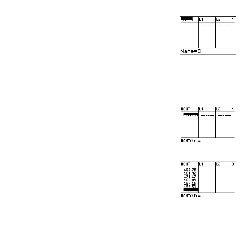
TI-83 Plus Inferential Statistics and Distributions 382
1. Press
…
Í
to display the stat list editor.
Press
}
to move the cursor onto
L1
, and then
press
y
6
. The
Name=
prompt is displayed
on the bottom line. The
Ø
cursor indicates that
alpha-lock is on. The existing list name columns
shift to the right.
Note: Your stat editor may not look like the one
pictured here, depending on the lists you have
already stored.
2. Enter [
H
] [
G
] [
H
] [
T
] at the
Name=
prompt, and
then press
Í
. The list to which you will
store the women’s height data is created.
Press
†
to move the cursor onto the first row of
the list.
HGHT(1)=
is displayed on the bottom line.
3. Press
169
Ë
43
to enter the first height value.
As you enter it, it is displayed on the bottom
line.
Press
Í
. The value is displayed in the first
row, and the rectangular cursor moves to the
next row.
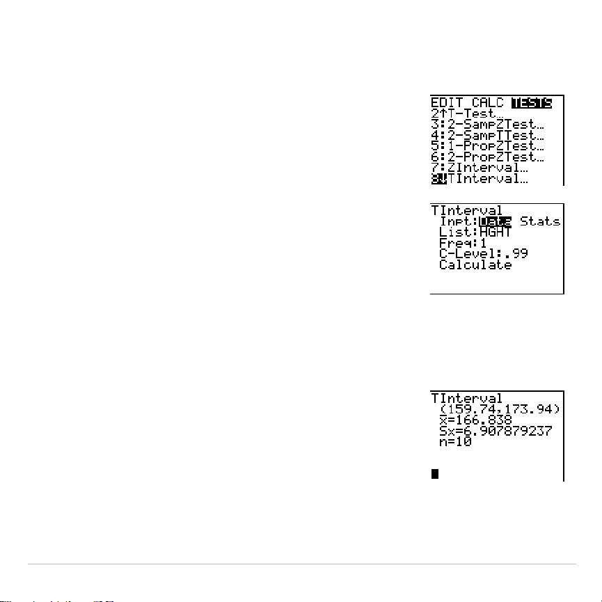
TI-83 Plus Inferential Statistics and Distributions 383
Enter the other nine height values the same
way.
4. Press
…
|
to display the
STAT TESTS
menu,
and then press
†
until
8:TInterval
is highlighted.
5. Press
Í
to select
8:TInterval
. The inferential
stat editor for
TInterval
is displayed. If
Data
is not
selected for
Inpt:
, press
|
Í
to select
Data
.
Press
†
and [
H
] [
G
] [
H
] [
T
] at the
List:
prompt
(alpha-lock is on).
Press
†
†
Ë
99
to enter a 99 percent
confidence level at the
C
.
Level:
prompt.
6. Press
†
to move the cursor onto
Calculate
, and
then press
Í
. The confidence interval is
calculated, and the
TInterval
results are
displayed on the home screen.

TI-83 Plus Inferential Statistics and Distributions 384
Interpret the results.
The first line,
(159.74,173.94)
, shows that the 99 percent confidence
interval for the population mean is between about 159.74 centimeters
and 173.94 centimeters. This is about a 14.2 centimeters spread.
The .99 confidence level indicates that in a very large number of
samples, we expect 99 percent of the intervals calculated to contain the
population mean. The actual mean of the population sampled is 165.1
centimeters, which is in the calculated interval.
The second line gives the mean height of the sample
þ
used to compute
this interval. The third line gives the sample standard deviation
Sx
. The
bottom line gives the sample size
n
.
To obtain a more precise bound on the population mean
m
of women’s
heights, increase the sample size to 90. Use a sample mean
þ
of 163.8
and sample standard deviation
Sx
of 7.1 calculated from the larger
random sample. This time, use the
Stats
(summary statistics) input
option.
7. Press
…
|
8
to display the inferential stat
editor for
TInterval
.
Press
~
Í
to select
Inpt:Stats
. The editor
changes so that you can enter summary
statistics as input.
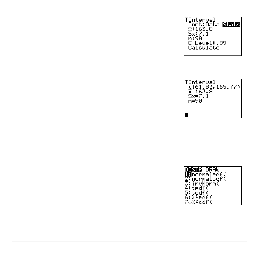
TI-83 Plus Inferential Statistics and Distributions 385
8. Press
†
163
Ë
8
Í
to store 163.8 to
ü
.
Press
7
Ë
1
Í
to store 7.1 to
Sx
.
Press
90
Í
to store 90 to
n
.
9. Press
†
to move the cursor onto
Calculate
, and
then press
Í
to calculate the new 99
percent confidence interval. The results are
displayed on the home screen.
If the height distribution among a population of women is normally
distributed with a mean
m
of 165.1 centimeters and a standard deviation
σ
of 6.35 centimeters, what height is exceeded by only 5 percent of the
women (the 95th percentile)?
10.Press
‘
to clear the home screen.
Press
y
=
to display the
DISTR
(distributions) menu.
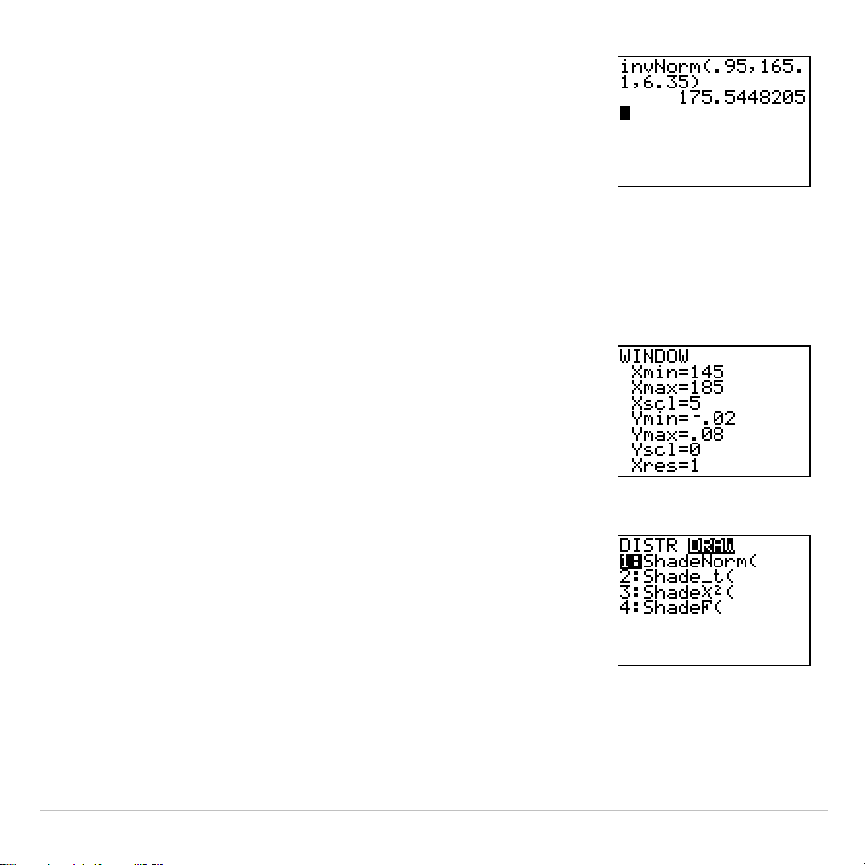
TI-83 Plus Inferential Statistics and Distributions 386
11. Press
3
to paste
invNorm(
to the home screen.
Press
Ë
95
¢
165
Ë
1
¢
6
Ë
35
¤
Í
.
.95
is the area,
165.1
is
µ
, and
6.35
is
σ
.
The result is displayed on the home screen; it shows that five percent of
the women are taller than 175.5 centimeters.
Now graph and shade the top 5 percent of the population.
12. Press
p
and set the window variables to
these values.
Xmin=145 Ymin=
L
.02 Xres=1
Xmax=185 Ymax=.08
Xscl=5 Yscl=0
13. Press
y
=
~
to display the
DISTR DRAW
menu.
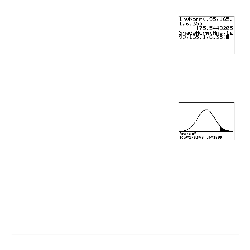
TI-83 Plus Inferential Statistics and Distributions 387
14. Press
Í
to paste
ShadeNorm(
to the home
screen.
Press
y
Z
¢
1
y
D
99
¢
165
Ë
1
¢
6
Ë
35
¤
.
Ans
(175.5448205 from step 11) is the lower
bound. 1
å
99 is the upper bound. The normal
curve is defined by a mean
µ
of 165.1 and a
standard deviation
σ
of 6.35.
15. Press
Í
to plot and shade the normal
curve.
Area
is the area above the 95th percentile.
low
is the lower bound.
up
is the upper bound.

TI-83 Plus Inferential Statistics and Distributions 388
Inferential Stat Editors
Displaying the Inferential Stat Editors
When you select a hypothesis test or confidence interval instruction from
the home screen, the appropriate inferential statistics editor is displayed.
The editors vary according to each test or interval’s input requirements.
Below is the inferential stat editor for
T-Test
.
Note: When you select the
ANOVA(
instruction, it is pasted to the home screen.
ANOVA(
does not have an editor screen.
Using an Inferential Stat Editor
To use an inferential stat editor, follow these steps.
1. Select a hypothesis test or confidence interval from the
STAT TESTS
menu. The appropriate editor is displayed.
2. Select
Data
or
Stats
input, if the selection is available. The appropriate
editor is displayed.
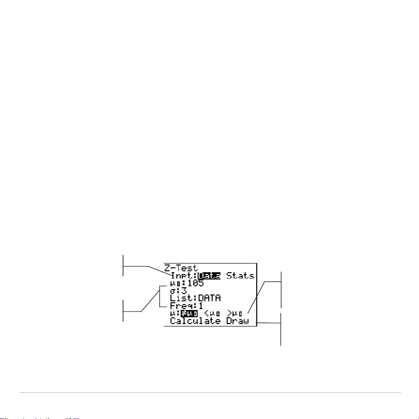
TI-83 Plus Inferential Statistics and Distributions 389
3. Enter real numbers, list names, or expressions for each argument in
the editor.
4. Select the alternative hypothesis (
ƒ
,
<
, or
>
) against which to test, if
the selection is available.
5. Select
No
or
Yes
for the
Pooled
option, if the selection is available.
6. Select
Calculate
or
Draw
(when
Draw
is available) to execute the
instruction.
•
When you select
Calculate
, the results are displayed on the home
screen.
•
When you select
Draw
, the results are displayed in a graph.
This chapter describes the selections in the above steps for each
hypothesis test and confidence interval instruction.
Enter values
for arguments
Select
Data
or
Stats
input
Select an
alternative
hypothesis
Select
Calculate
or
Draw
output

TI-83 Plus Inferential Statistics and Distributions 390
Selecting Data or Stats
Most inferential stat editors prompt you to select one of two types of
input. (
1
.
PropZInt
and
2
.
PropZTest
,
1
.
PropZInt
and
2
.
PropZInt
,
c
2
.
Test
, and
LinRegTTest
do not.)
•
Select
Data
to enter the data lists as input.
•
Select
Stats
to enter summary statistics, such as
þ
,
Sx
, and
n
, as
input.
To select
Data
or
Stats
, move the cursor to either
Data
or
Stats
, and then
press
Í
.
Entering the Values for Arguments
Inferential stat editors require a value for every argument. If you do not
know what a particular argument symbol represents, see the
Inferential
Statistics Input Descriptions tables
.
When you enter values in any inferential stat editor, the TI-83 Plus stores
them in memory so that you can run many tests or intervals without
having to reenter every value.

TI-83 Plus Inferential Statistics and Distributions 391
Selecting an Alternative Hypothesis (
ƒ
< >)
Most of the inferential stat editors for the hypothesis tests prompt you to
select one of three alternative hypotheses.
•
The first is a
ƒ
alternative hypothesis, such as
mƒm
0
for the
Z
.
Test
.
•
The second is a
<
alternative hypothesis, such as
m
1<
m
2
for the
2
.
SampTTest
.
•
The third is a
>
alternative hypothesis, such as
p1>p2
for the
2
.
PropZTest
.
To select an alternative hypothesis, move the cursor to the appropriate
alternative, and then press
Í
.
Selecting the Pooled Option
Pooled
(
2
.
SampTTest
and
2
.
SampTInt
only) specifies whether the
variances are to be pooled for the calculation.
•
Select
No
if you do not want the variances pooled. Population
variances can be unequal.
•
Select
Yes
if you want the variances pooled. Population variances are
assumed to be equal.
To select the
Pooled
option, move the cursor to
Yes
, and then press
Í
.

TI-83 Plus Inferential Statistics and Distributions 392
Selecting Calculate or Draw for a Hypothesis Test
After you have entered all arguments in an inferential stat editor for a
hypothesis test, you must select whether you want to see the calculated
results on the home screen (
Calculate
) or on the graph screen (
Draw
).
•
Calculate
calculates the test results and displays the outputs on the
home screen.
•
Draw
draws a graph of the test results and displays the test statistic
and p-value with the graph. The window variables are adjusted
automatically to fit the graph.
To select
Calculate
or
Draw
, move the cursor to either
Calculate
or
Draw
,
and then press
Í
. The instruction is immediately executed.
Selecting Calculate for a Confidence Interval
After you have entered all arguments in an inferential stat editor for a
confidence interval, select
Calculate
to display the results. The
Draw
option is not available.
When you press
Í
,
Calculate
calculates the confidence interval
results and displays the outputs on the home screen.
TI-83 Plus Inferential Statistics and Distributions 393
Bypassing the Inferential Stat Editors
To paste a hypothesis test or confidence interval instruction to the home
screen without displaying the corresponding inferential stat editor, select
the instruction you want from the
CATALOG
menu. Appendix A describes
the input syntax for each hypothesis test and confidence interval
instruction.
Note: You can paste a hypothesis test or confidence interval instruction to a
command line in a program. From within the program editor, select the
instruction from either the
CATALOG
(Chapter 15) or the
STAT TESTS
menu.
TI-83 Plus Inferential Statistics and Distributions 394
STAT TESTS Menu
STAT TESTS Menu
To display the
STAT TESTS
menu, press
…
|
. When you select an
inferential statistics instruction, the appropriate inferential stat editor is
displayed.
Most
STAT TESTS
instructions store some output variables to memory. For
a list of these variables, see the Test and Interval Output Variables table.
EDIT CALC TESTS
1: Z-Test...
Test for 1
m
, known
s
2: T-Test...
Test for 1
m
, unknown
s
3: 2-SampZTest...
Test comparing 2
m
’s, known
s
’s
4: 2-SampTTest...
Test comparing 2
m
’s, unknown
s
’s
5: 1-PropZTest...
Test for 1 proportion
6: 2-PropZTest...
Test comparing 2 proportions
7: ZInterval...
Confidence interval for 1
m
, known
s
8: TInterval...
Confidence interval for 1
m
, unknown
s
9: 2-SampZInt...
Confidence interval for difference of 2
m
’s, known
s
’s
0: 2-SampTInt...
Confidence interval for difference of 2
m
’s, unknown
s
’s
A: 1-PropZInt...
Confidence interval for 1 proportion
B: 2-PropZInt...
Confidence interval for difference of 2 proportions
C:
c
2-Test...
Chi-square test for 2-way tables
D: 2-SampÛTest...
Test comparing 2
s
’s
TI-83 Plus Inferential Statistics and Distributions 395
EDIT CALC TESTS
E: LinRegTTest...
t
test for regression slope and
r
F: ANOVA(
One-way analysis of variance
Note:
When a new test or interval is computed, all previous output variables are
invalidated.
Inferential Stat Editors for the STAT TESTS Instructions
In this chapter, the description of each
STAT TESTS
instruction shows the
unique inferential stat editor for that instruction with example arguments.
•
Descriptions of instructions that offer the
Data
/
Stats
input choice show
both types of input screens.
•
Descriptions of instructions that do not offer the
Data
/
Stats
input
choice show only one input screen.
The description then shows the unique output screen for that instruction
with the example results.
•
Descriptions of instructions that offer the
Calculate
/
Draw
output choice
show both types of screens: calculated and graphic results.
•
Descriptions of instructions that offer only the
Calculate
output choice
show the calculated results on the home screen.
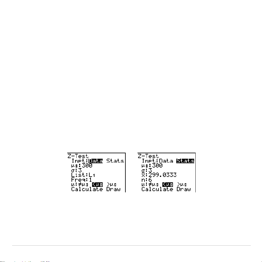
TI-83 Plus Inferential Statistics and Distributions 396
Z
.
Test
Z
.
Test
(one-sample
z
test; item
1
) performs a hypothesis test for a single
unknown population mean
m
when the population standard deviation
s
is
known. It tests the null hypothesis H
0
:
m
=
m
0
against one of the
alternatives below.
•
H
a
:
mƒm
0
(
m
:
ƒm
0
)
•
H
a
:
m
<
m
0
(
m
:<
m
0
)
•
H
a
:
m
>
m
0
(
m
:>
m
0
)
In the example:
L1={299.4 297.7 301 298.9 300.2 297}
Data Stats
Input:
,,
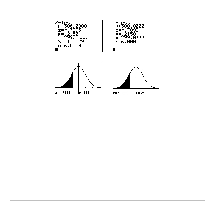
TI-83 Plus Inferential Statistics and Distributions 397
Data Stats
Calculated results:
,,
Drawn results:
Note:
All
STAT TESTS
examples assume a fixed-decimal mode setting of
4
(Chapter 1). If you set the decimal mode to
Float
or a different fixed-decimal
setting, your output may differ from the output in the examples.
T
.
Test
T
.
Test
(one-sample
t
test; item
2
) performs a hypothesis test for a single
unknown population mean
m
when the population standard deviation
s
is
unknown. It tests the null hypothesis H
0
:
m
=
m
0
against one of the
alternatives below.
•
H
a
:
mƒm
0
(
m
:
ƒm
0
)
•
H
a
:
m
<
m
0
(
m
:<
m
0
)
•
H
a
:
m
>
m
0
(
m
:>
m
0
)
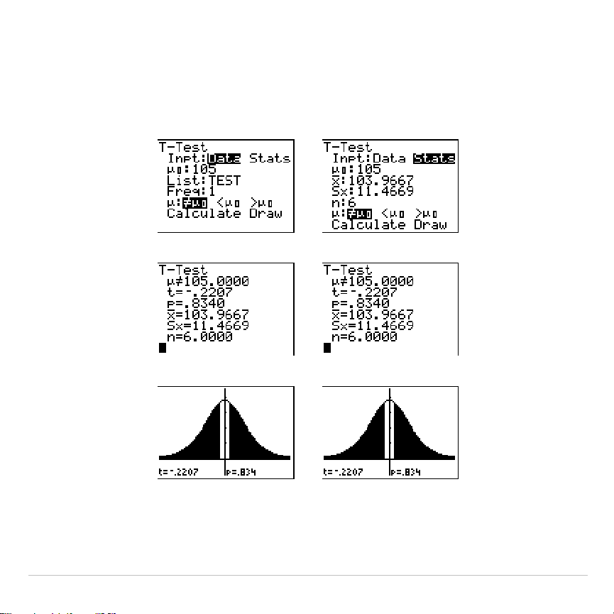
TI-83 Plus Inferential Statistics and Distributions 398
In the example:
TEST={91.9 97.8 111.4 122.3 105.4 95}
Data Stats
Input:
,,
Calculated results:
,,
Drawn results:
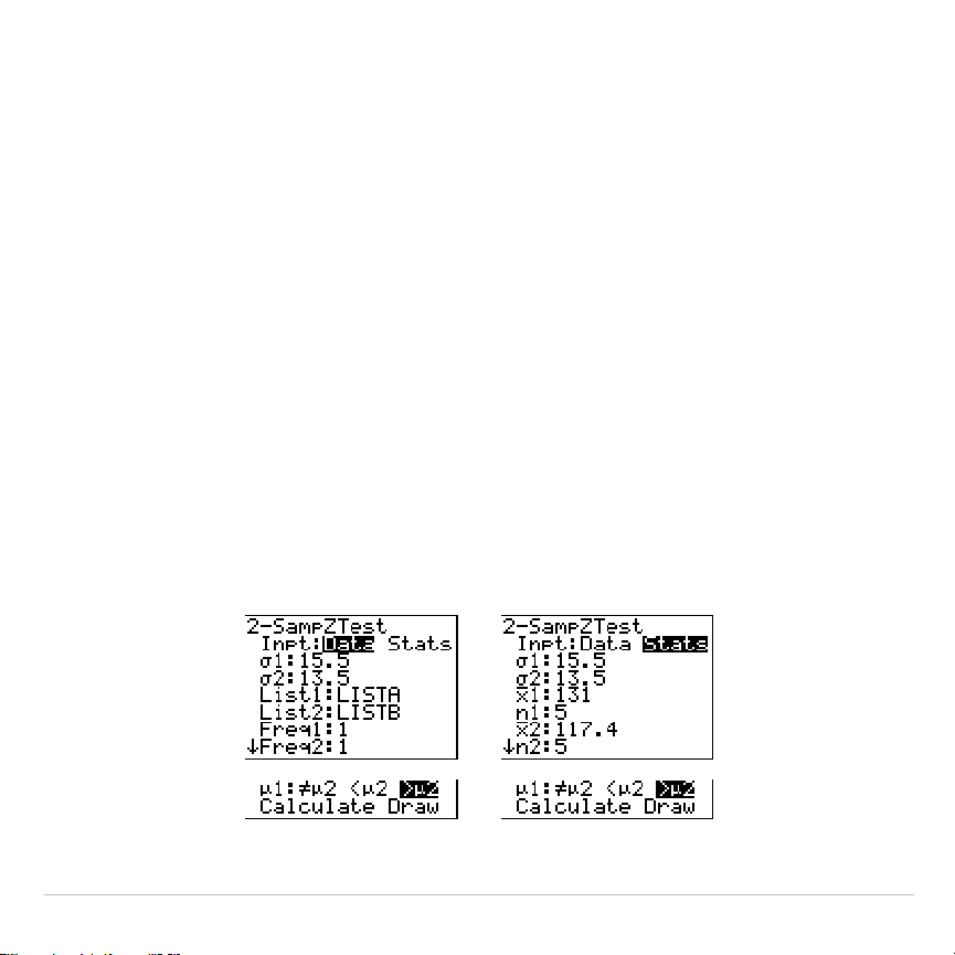
TI-83 Plus Inferential Statistics and Distributions 399
2
.
SampZTest
2
.
SampZTest
(two-sample
z
test; item
3
) tests the equality of the means of
two populations (
m
1
and
m
2
) based on independent samples when both
population standard deviations (
s
1
and
s
2
) are known. The null
hypothesis H
0
:
m
1
=
m
2
is tested against one of the alternatives below.
•
H
a
:
m
1
ƒm
2
(
m
1:
ƒm
2
)
•
H
a
:
m
1
<
m
2
(
m
1:<
m
2
)
•
H
a
:
m
1
>
m
2
(
m
1:>
m
2
)
In the example:
LISTA={154 109 137 115 140}
LISTB={108 115 126 92 146}
Data Stats
Input:
,,
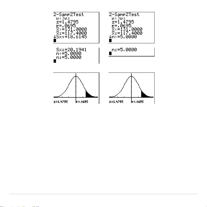
TI-83 Plus Inferential Statistics and Distributions 400
Calculated results:
,
,
Drawn results:
2
.
SampTTest
2
.
SampTTest
(two-sample
t
test; item
4
) tests the equality of the means of
two populations (
m
1
and
m
2
) based on independent samples when
neither population standard deviation (
s
1
or
s
2
) is known. The null
hypothesis H
0
:
m
1
=
m
2
is tested against one of the alternatives below.
•
H
a
:
m
1
ƒm
2
(
m
1:
ƒm
2
)
•
H
a
:
m
1
<
m
2
(
m
1:<
m
2
)
•
H
a
:
m
1
>
m
2
(
m
1:>
m
2
)
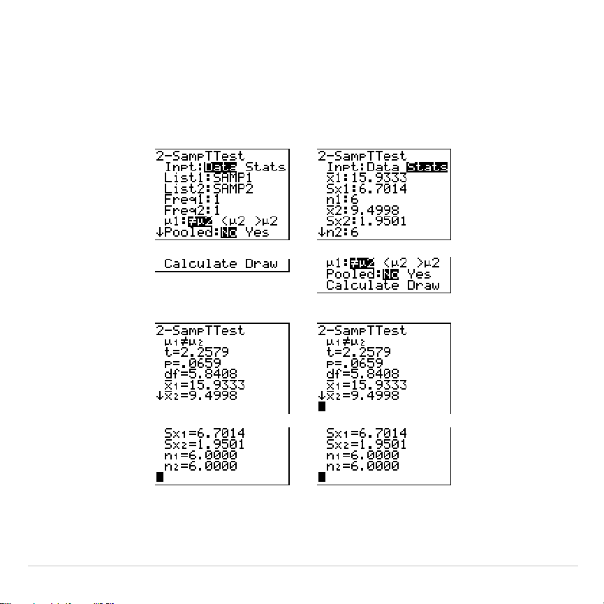
TI-83 Plus Inferential Statistics and Distributions 401
In the example:
SAMP1={12.207 16.869 25.05 22.429 8.456 10.589}
SAMP2={11.074 9.686 12.064 9.351 8.182 6.642}
Data Stats
Input:
,,
Calculated results:
,,
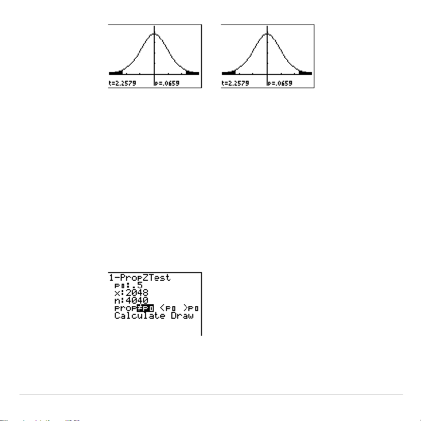
TI-83 Plus Inferential Statistics and Distributions 402
Drawn results:
1
.
PropZTest
1
.
PropZTest
(one-proportion
z
test; item
5
) computes a test for an
unknown proportion of successes (prop). It takes as input the count of
successes in the sample
x
and the count of observations in the sample
n
.
1
.
PropZTest
tests the null hypothesis H
0
: prop=p
0
against one of the
alternatives below.
•
H
a
: prop
ƒ
p
0
(
prop:
ƒ
p0
)
•
H
a
: prop<p
0
(
prop:<p0
)
•
H
a
: prop>p
0
(
prop:>p0
)
Input:
,
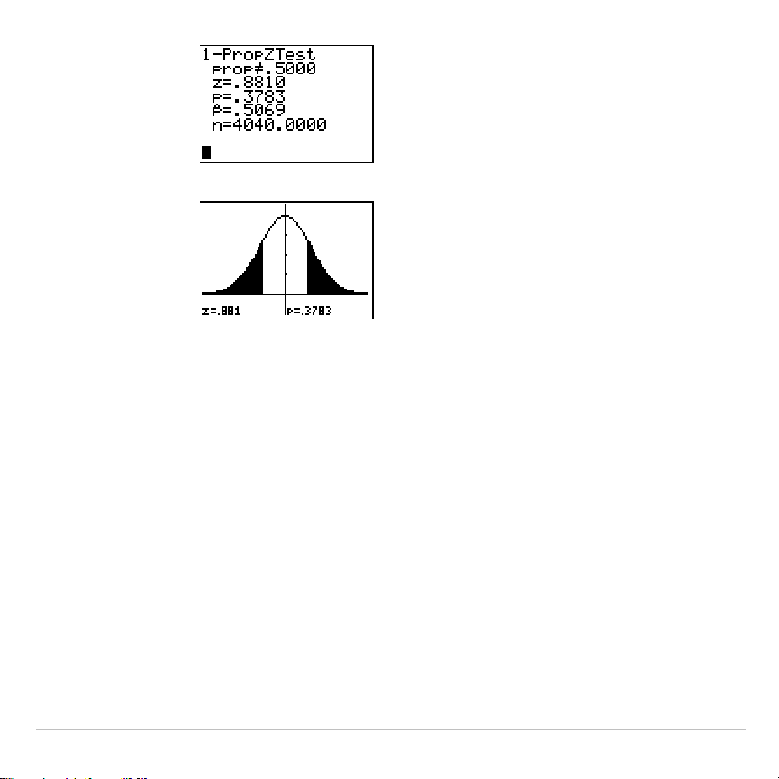
TI-83 Plus Inferential Statistics and Distributions 403
Calculated results:
,
Drawn results:
2
.
PropZTest
2
.
PropZTest
(two-proportion
z
test; item
6
) computes a test to compare
the proportion of successes (p
1
and p
2
) from two populations. It takes as
input the count of successes in each sample (
x
1
and
x
2
) and the count of
observations in each sample (
n
1
and
n
2
).
2
.
PropZTest
tests the null
hypothesis H
0
: p
1
=p
2
(using the pooled sample proportion
Ç
) against
one of the alternatives below.
•
H
a
: p
1
ƒ
p
2
(
p1:
ƒ
p2
)
•
H
a
: p
1
<p
2
(
p1:<p2
)
•
H
a
: p
1
>p
2
(
p1:>p2
)
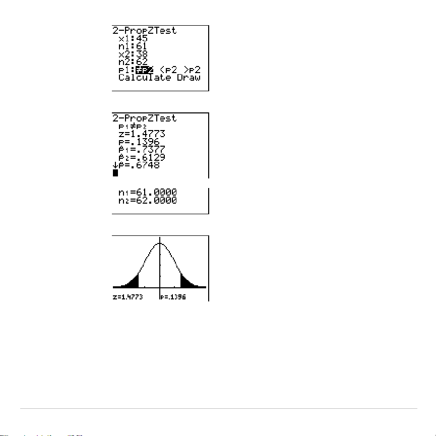
TI-83 Plus Inferential Statistics and Distributions 404
Input:
,
Calculated results:
,
Drawn results:
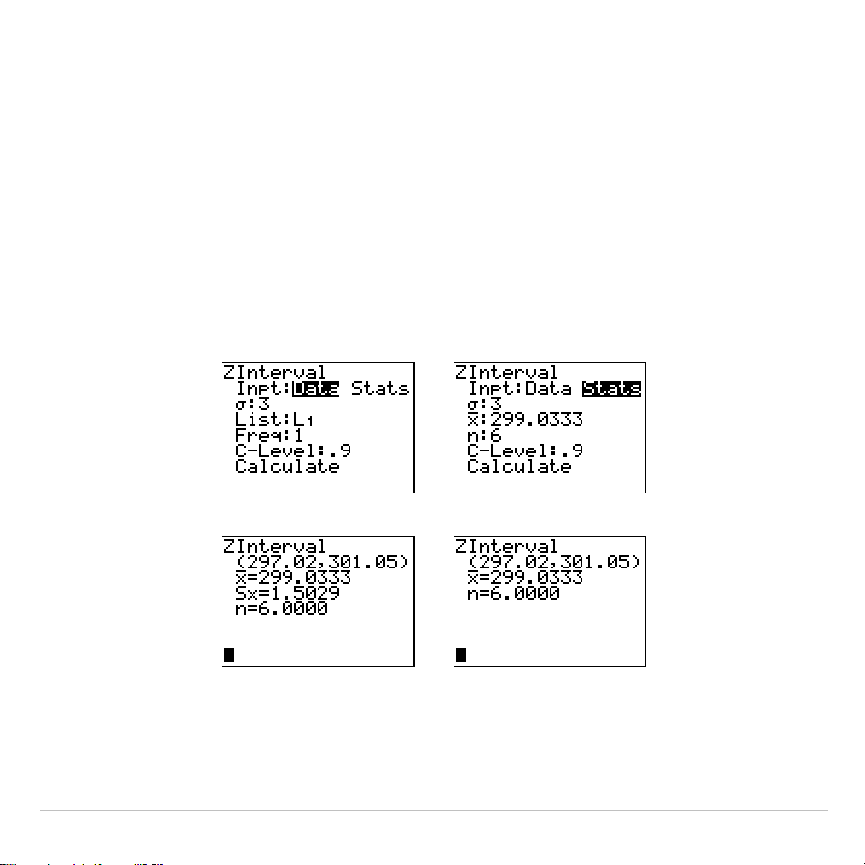
TI-83 Plus Inferential Statistics and Distributions 405
ZInterval
ZInterval
(one-sample
z
confidence interval; item
7
) computes a
confidence interval for an unknown population mean
m
when the
population standard deviation
s
is known. The computed confidence
interval depends on the user-specified confidence level.
In the example:
L1={299.4 297.7 301 298.9 300.2 297}
Data Stats
Input:
,,
Calculated results:
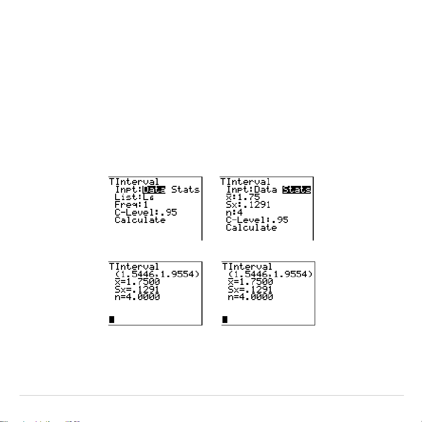
TI-83 Plus Inferential Statistics and Distributions 406
TInterval
TInterval
(one-sample
t
confidence interval; item
8
) computes a
confidence interval for an unknown population mean
m
when the
population standard deviation
s
is unknown. The computed confidence
interval depends on the user-specified confidence level.
In the example:
L6={1.6 1.7 1.8 1.9}
Data Stats
Input:
,,
Calculated results:
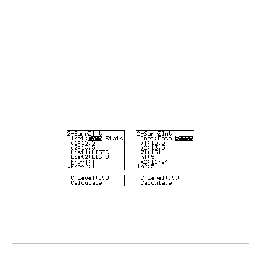
TI-83 Plus Inferential Statistics and Distributions 407
2
.
SampZInt
2
.
SampZInt
(two-sample
z
confidence interval; item
9
) computes a
confidence interval for the difference between two population means
(
m
1
Nm
2
) when both population standard deviations (
s
1
and
s
2
) are
known. The computed confidence interval depends on the user-specified
confidence level.
In the example:
LISTC={154 109 137 115 140}
LISTD={108 115 126 92 146}
Data Stats
Input:
,,
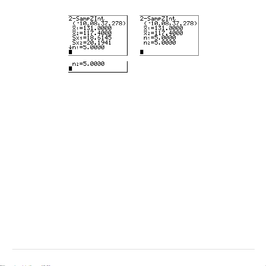
TI-83 Plus Inferential Statistics and Distributions 408
Calculated results:
2
.
SampTInt
2
.
SampTInt
(two-sample
t
confidence interval; item
0
) computes a
confidence interval for the difference between two population means
(
m
1
Nm
2
) when both population standard deviations (
s
1
and
s
2
) are
unknown. The computed confidence interval depends on the user-
specified confidence level.
In the example:
SAMP1={12.207 16.869 25.05 22.429 8.456 10.589}
SAMP2={11.074 9.686 12.064 9.351 8.182 6.642}
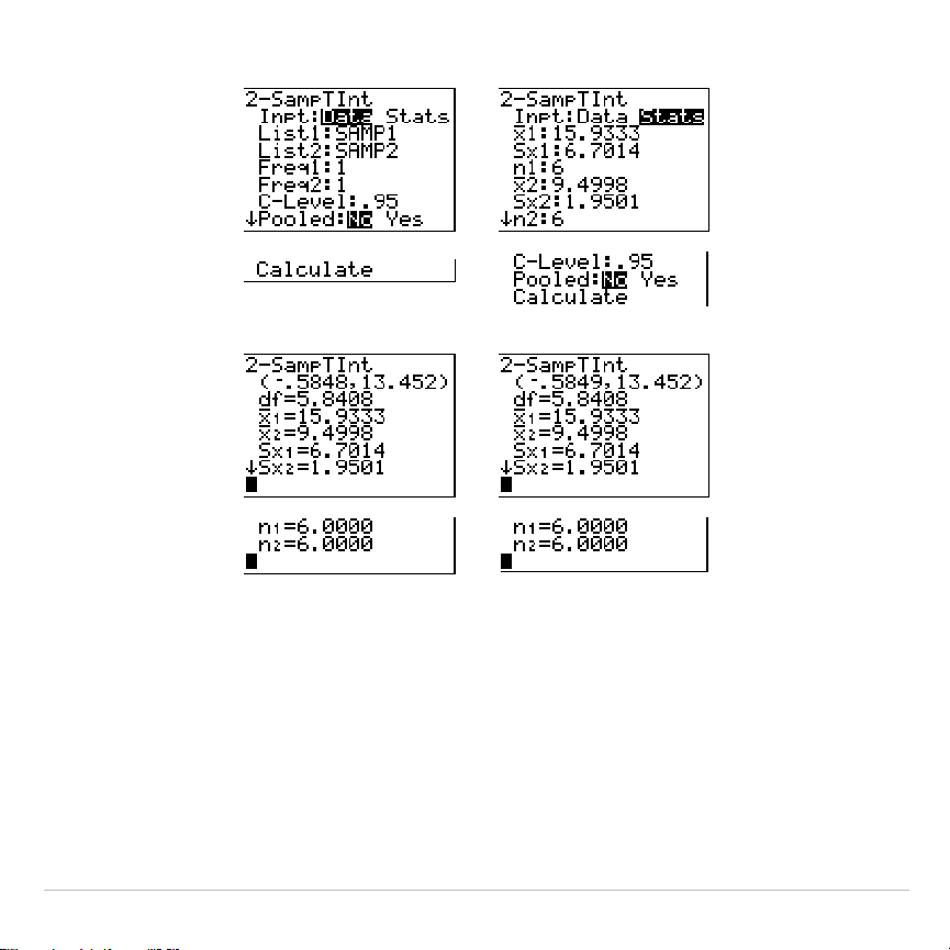
TI-83 Plus Inferential Statistics and Distributions 409
Data Stats
Input:
,,
Calculated results:
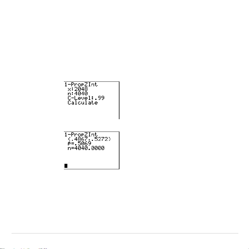
TI-83 Plus Inferential Statistics and Distributions 410
1
.
PropZInt
1
.
PropZInt
(one-proportion
z
confidence interval; item
A
) computes a
confidence interval for an unknown proportion of successes. It takes as
input the count of successes in the sample
x
and the count of
observations in the sample
n
. The computed confidence interval depends
on the user-specified confidence level.
Input:
,
Calculated results:
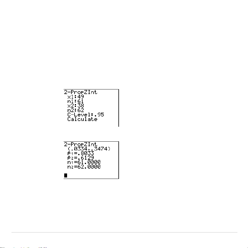
TI-83 Plus Inferential Statistics and Distributions 411
2
.
PropZInt
2
.
PropZInt
(two-proportion
z
confidence interval; item
B
) computes a
confidence interval for the difference between the proportion of
successes in two populations (p
1
N
p
2
). It takes as input the count of
successes in each sample (
x
1
and
x
2
) and the count of observations in
each sample
(
n
1
and
n
2
). The computed confidence interval depends on
the user-specified confidence level.
Input:
,
Calculated results:
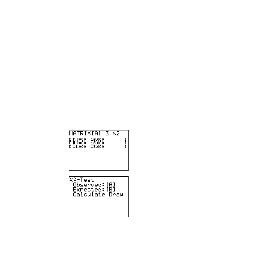
TI-83 Plus Inferential Statistics and Distributions 412
c
2
.
Test
c
2
.
Test
(chi-square test; item
C
) computes a chi-square test for
association on the two-way table of counts in the specified
Observed
matrix. The null hypothesis H
0
for a two-way table is: no association
exists between row variables and column variables. The alternative
hypothesis is: the variables are related.
Before computing a
c
2
.
Test, enter the observed counts in a matrix. Enter
that matrix variable name at the
Observed:
prompt in the
c
2
.
Test editor;
default=
[A]
. At the
Expected:
prompt, enter the matrix variable name to
which you want the computed expected counts to be stored; default=
[B]
.
Matrix editor:
Note:
Press
y
~
~
1
to select
1:
[A]
from the MATRX EDIT
menu.
Input:
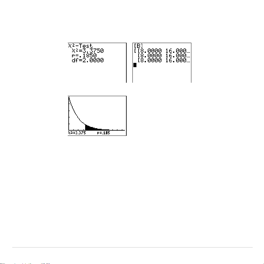
TI-83 Plus Inferential Statistics and Distributions 413
,
Note:
Press
y
[B]
Í
to display
matrix
[B]
.
Calculated results:
,
Drawn results:
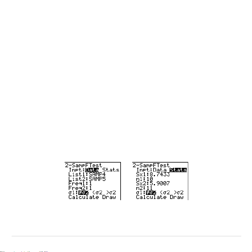
TI-83 Plus Inferential Statistics and Distributions 414
2
.
Samp
Ü
Test
2
.
Samp
Ü
Test
(two-sample
Û
-test; item
D
) computes an
Û
-test to compare
two normal population standard deviations (
s
1
and
s
2
). The population
means and standard deviations are all unknown.
2
.
Samp
Ü
Test
, which
uses the ratio of sample variances Sx1
2
/Sx2
2
, tests the null hypothesis
H
0
:
s
1
=
s
2
against one of the alternatives below.
•
H
a
:
s
1
ƒs
2
(
s
1:
ƒs
2
)
•
H
a
:
s
1
<
s
2
(
s
1:<
s
2
)
•
H
a
:
s
1
>
s
2
(
s
1:>
s
2
)
In the example:
SAMP4={ 7
L
41817
L
3
L
5 11011
L
2}
SAMP5={
L
112
L
1
L
33
L
552
L
11
L
1
L
3}
Data Stats
Input:
,,
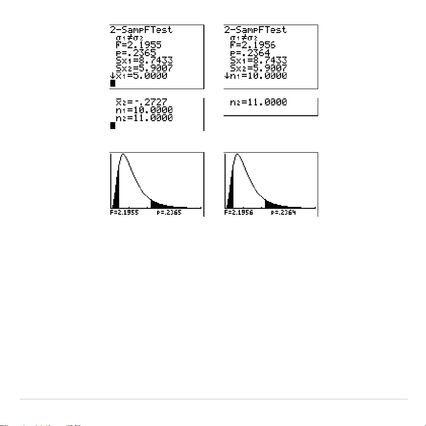
TI-83 Plus Inferential Statistics and Distributions 415
Calculated results:
,,
Drawn results:
LinRegTTest
LinRegTTest
(linear regression
t
test; item
E
) computes a linear
regression on the given data and a
t
test on the value of slope
b
and the
correlation coefficient
r
for the equation
y
=
a
+
b
x. It tests the null
hypothesis H
0
:
b
=0 (equivalently,
r
=0) against one of the alternatives
below.
•
H
a
:
bƒ
0 and
rƒ
0 (
b
&
r
:
ƒ
0
)
•
H
a
:
b
<0 and
r
<0 (
b
&
r
:<0
)
•
H
a
:
b
>0 and
r
>0 (
b
&
r
:>0
)
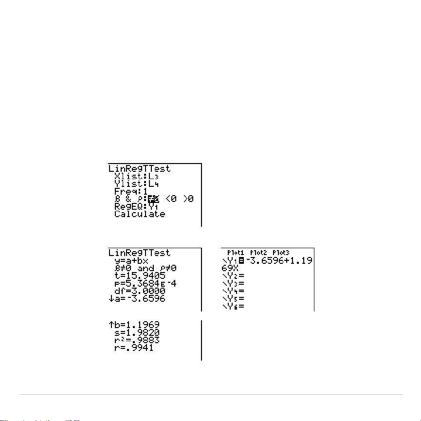
TI-83 Plus Inferential Statistics and Distributions 416
The regression equation is automatically stored to
RegEQ
(
VARS Statistics
EQ
secondary menu). If you enter a
Y=
variable name at the
RegEQ:
prompt, the calculated regression equation is automatically stored to the
specified
Y=
equation. In the example below, the regression equation is
stored to
Y1
, which is then selected (turned on).
In the example:
L3={ 3856596474}
L
4={ 4163707284}
Input:
,
Calculated results:

TI-83 Plus Inferential Statistics and Distributions 417
When
LinRegTTest
is executed, the list of residuals is created and stored
to the list name
RESID
automatically.
RESID
is placed on the
LIST NAMES
menu.
Note: For the regression equation, you can use the fix-decimal mode setting to
control the number of digits stored after the decimal point (Chapter 1).
However, limiting the number of digits to a small number could affect the
accuracy of the fit.
ANOVA(
ANOVA(
(one-way analysis of variance; item
F
) computes a one-way
analysis of variance for comparing the means of two to 20 populations.
The
ANOVA
procedure for comparing these means involves analysis of
the variation in the sample data. The null hypothesis H
0
:
m
1
=
m
2
=...=
m
k
is
tested against the alternative H
a
: not all
m
1
...
m
k
are equal.
ANOVA(
list1
,
list2
[
,
...
,
list20
]
)
In the example:
L1={7 4 6 6 5}
L
2={6 5 5 8 7}
L
3={4 7 6 7 6}
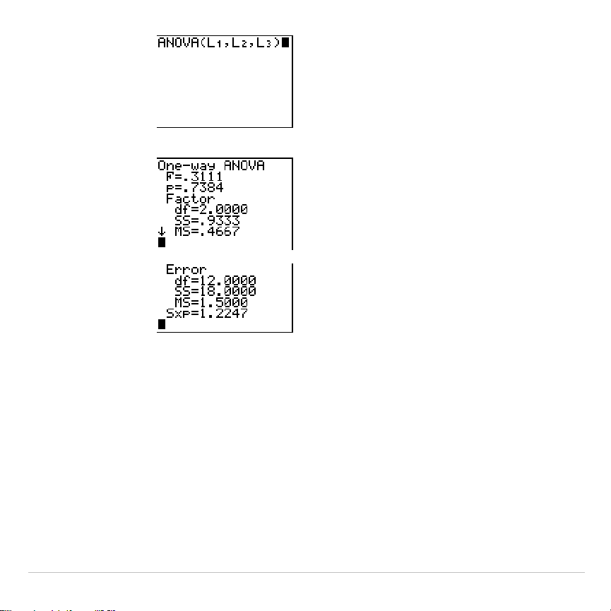
TI-83 Plus Inferential Statistics and Distributions 418
Input:
,
Calculated results:
Note:
SS
is sum of squares and
MS
is mean square.

TI-83 Plus Inferential Statistics and Distributions 419
Inferential Statistics Input Descriptions
The tables in this section describe the inferential statistics inputs
discussed in this chapter. You enter values for these inputs in the
inferential stat editors. The tables present the inputs in the same order
that they appear in this chapter.
Input Description
m
0
Hypothesized value of the population mean that you are
testing.
s
The known population standard deviation; must be a real
number > 0.
List
The name of the list containing the data you are testing.
Freq
The name of the list containing the frequency values for
the data in
List
. Default=1. All elements must be integers
|
0.
Calculate
/
Draw
Determines the type of output to generate for tests and
intervals.
Calculate
displays the output on the home
screen. In tests,
Draw
draws a graph of the results.
v
,
Sx
,
n
Summary statistics (mean, standard deviation, and
sample size) for the one-sample tests and intervals.
s
1
The known population standard deviation from the first
population for the two-sample tests and intervals. Must
be a real number > 0.
TI-83 Plus Inferential Statistics and Distributions 420
Input Description
s
2
The known population standard deviation from the
second population for the two-sample tests and intervals.
Must be a real number > 0.
List1
,
List2
The names of the lists containing the data you are testing
for the two-sample tests and intervals. Defaults are
L1
and
L2
, respectively.
Freq1
,
Freq2
The names of the lists containing the frequencies for the
data in
List1
and
List2
for the two-sample tests and
intervals. Defaults=1. All elements must be integers
|
0.
v
1
,
Sx1
,
n
1
,
v
2
,
Sx2
,
n
2
Summary statistics (mean, standard deviation, and
sample size) for sample one and sample two in the two-
sample tests and intervals.
Pooled
Specifies whether variances are to be pooled for
2
.
SampTTest
and
2
.
SampTInt. No
instructs the TI
.
83 not to
pool the variances.
Yes
instructs the TI
.
83 to pool the
variances.
p
0
The expected sample proportion for
1
.
PropZTest
. Must be
a real number, such that 0 <
p
0
< 1.
x
The count of successes in the sample for the
1
.
PropZTest
and
1
.
PropZInt.
Must be an integer
‚
0.
n
The count of observations in the sample for the
1
.
PropZTest
and
1
.
PropZInt
. Must be an integer > 0.
x1
The count of successes from sample one for the
2
.
PropZTest
and
2
.
PropZInt
. Must be an integer
‚
0.

TI-83 Plus Inferential Statistics and Distributions 421
Input Description
x2
The count of successes from sample two for the
2
.
PropZTest
and
2
.
PropZInt
. Must be an integer
‚
0.
n1
The count of observations in sample one for the
2
.
PropZTest
and
2
.
PropZInt
. Must be an integer > 0.
n2
The count of observations in sample two for the
2
.
PropZTest
and
2
.
PropZInt
. Must be an integer > 0.
C
.
Level
The confidence level for the interval instructions. Must be
‚
0 and <100. If it is
‚
1, it is assumed to be given as a
percent and is divided by 100. Default=0.95.
Observed (Matrix)
The matrix name that represents the columns and rows
for the observed values of a two-way table of counts for
the
c
2
.
Test
.
Observed
must contain all integers
‚
0. Matrix
dimensions must be at least 2×2.
Expected (Matrix)
The matrix name that specifies where the expected
values should be stored.
Expected
is created upon
successful completion of the
c
2
.
Test
.
Xlist
,
Ylist
The names of the lists containing the data for
LinRegTTest
.
Defaults are
L1
and
L2
, respectively. The dimensions of
Xlist
and
Ylist
must be the same.
RegEQ
The prompt for the name of the
Y=
variable where the
calculated regression equation is to be stored. If a
Y=
variable is specified, that equation is automatically
selected (turned on). The default is to store the
regression equation to the
RegEQ
variable only.

TI-83 Plus Inferential Statistics and Distributions 422
Test and Interval Output Variables
The inferential statistics variables are calculated as indicated below. To
access these variables for use in expressions, press
,
5
(
5:Statistics
), and then select the
VARS
menu listed in the last column
below.
Variables Tests Intervals
LinRegTTest
ANOVA
VARS
Menu
p-value
p p TEST
test statistics
z, t,
c
2,
Ü
t,
Ü
TEST
degrees of freedom
df df df TEST
sample mean of x values for sample
1 and sample 2
v
1,
v
2
v
1,
v
2 TEST
sample standard deviation of x for
sample 1 and sample 2
Sx1,
Sx2
Sx1,
Sx2
TEST
number of data points for sample 1
and sample 2
n1, n2 n1, n2 TEST
pooled standard deviation
SxP SxP SxP TEST
estimated sample proportion
ÇÇ
TEST
estimated sample proportion for
population 1
Ç
1
Ç
1 TEST
estimated sample proportion for
population 2
Ç
2
Ç
2 TEST

TI-83 Plus Inferential Statistics and Distributions 423
Variables Tests Intervals
LinRegTTest
ANOVA
VARS
Menu
confidence interval pair
lower,
upper
TEST
mean of x values
vv
XY
sample standard deviation of x
Sx Sx XY
number of data points
nn XY
standard error about the line
s TEST
regression/fit coefficients
a, b EQ
correlation coefficient
rEQ
coefficient of determination
r2 EQ
regression equation
RegEQ EQ
Note: The variables listed above cannot be archived.

TI-83 Plus Inferential Statistics and Distributions 424
Distribution Functions
DISTR menu
To display the
DISTR
menu, press
y
=
.
DISTR DRAW
1:normalpdf(
Normal probability density
2:normalcdf(
Normal distribution probability
3:invNorm(
Inverse cumulative normal distribution
4:tpdf(
Student-
t
probability density
5:tcdf(
Student-
t
distribution probability
6:
c
2
pdf(
Chi-square probability density
7:
c
2
cdf
Chi-square distribution probability
8:
Ü
pdf(
Û
probability density
9:
Ü
cdf(
Û
distribution probability
0:binompdf(
Binomial probability
A:binomcdf(
Binomial cumulative density
B:poissonpdf(
Poisson probability
C:poissoncdf(
Poisson cumulative density
D:geometpdf(
Geometric probability
E:geometcdf(
Geometric cumulative density
Note:
L
1
å
99 and 1
å
99 specify infinity. If you want to view the area left of
upperbound
, for example, specify
lowerbound
=
L
1
å
99.
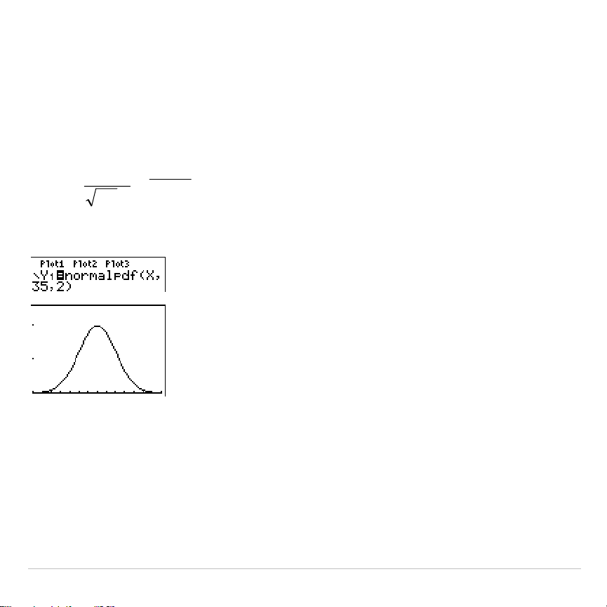
TI-83 Plus Inferential Statistics and Distributions 425
normalpdf(
normalpdf(
computes the probability density function (
pdf
) for the normal
distribution at a specified
x
value. The defaults are mean
m
=0 and
standard deviation
s
=1. To plot the normal distribution, paste
normalpdf(
to the
Y=
editor. The probability density function (pdf) is:
0,
2
1
)(
2
2
2
)(
>=
−
−
σ
σπ
σ
µ
x
exf
normalpdf(
x
[
,
m
,
s
]
)
Note: For this example,
Xmin = 28
Xmax = 42
Ymin = 0
Ymax = .25
Tip: For plotting the normal distribution, you can set window variables
Xmin
and
Xmax
so that the mean
m
falls between them, and then select
0:ZoomFit
from the
ZOOM
menu.
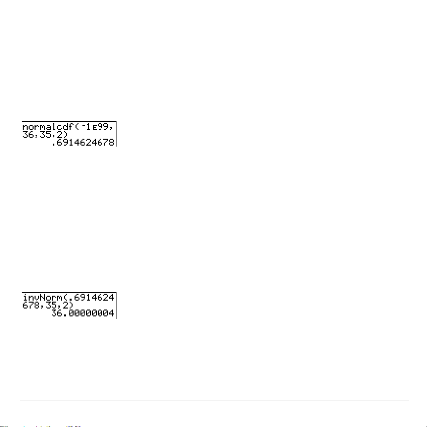
TI-83 Plus Inferential Statistics and Distributions 426
normalcdf(
normalcdf(
computes the normal distribution probability between
lowerbound
and
upperbound
for the specified mean
m
and standard
deviation
s
. The defaults are
m
=0 and
s
=1.
normalcdf(
lowerbound
,
upperbound
[
,
m
,
s
]
)
invNorm(
invNorm(
computes the inverse cumulative normal distribution function
for a given
area
under the normal distribution curve specified by mean
m
and standard deviation
s
. It calculates the
x
value associated with an
area
to the left of the
x
value. 0
area
1 must be true. The defaults are
m
=0
and
s
=1.
invNorm(
area
[
,
m
,
s
]
)
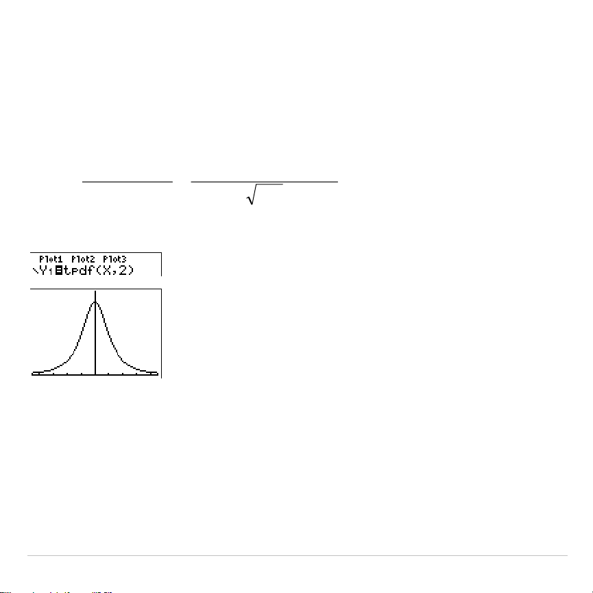
TI-83 Plus Inferential Statistics and Distributions 427
tpdf(
tpdf(
computes the probability density function (pdf) for the Student-
t
distribution at a specified
x
value.
df
(degrees of freedom) must be >0. To
plot the Student-
t
distribution, paste
tpdf(
to the
Y=
editor. The probability
density function (pdf)
is:
df
dfx
df
df
xf
df
π
2/)1(
2
)/1(
)2/(
]2/)1[(
)(
+−
+
Γ
+Γ
=
tpdf(
x
,
df
)
Note: For this example,
Xmin =
L
4.5
Xmax = 4.5
Ymin = 0
Ymax = .4
tcdf(
tcdf(
computes the Student-
t
distribution probability between
lowerbound
and
upperbound
for the specified
df
(degrees of freedom), which must be
> 0.
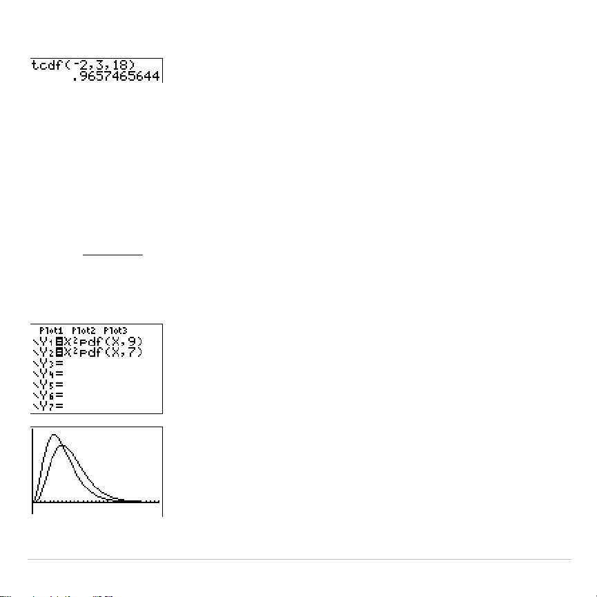
TI-83 Plus Inferential Statistics and Distributions 428
tcdf(
lowerbound
,
upperbound
,
df
)
c
2
pdf(
c
2
pdf(
computes the probability density function (pdf) for the
c
2
(chi-square) distribution at a specified
x
value.
df
(degrees of freedom)
must be an integer > 0. To plot the
c
2
distribution, paste
c
2
pdf(
to the
Y=
editor. The probability density function (pdf) is:
0,2)/(1
)2/(
1
)(
2/12/2/
≥
Γ
=
−−
xex
df
xf
xdfdf
c
2
pdf(
x
,
df
)
Note: For this example,
Xmin = 0
Xmax = 30
Ymin =
L
.02
Ymax = .132
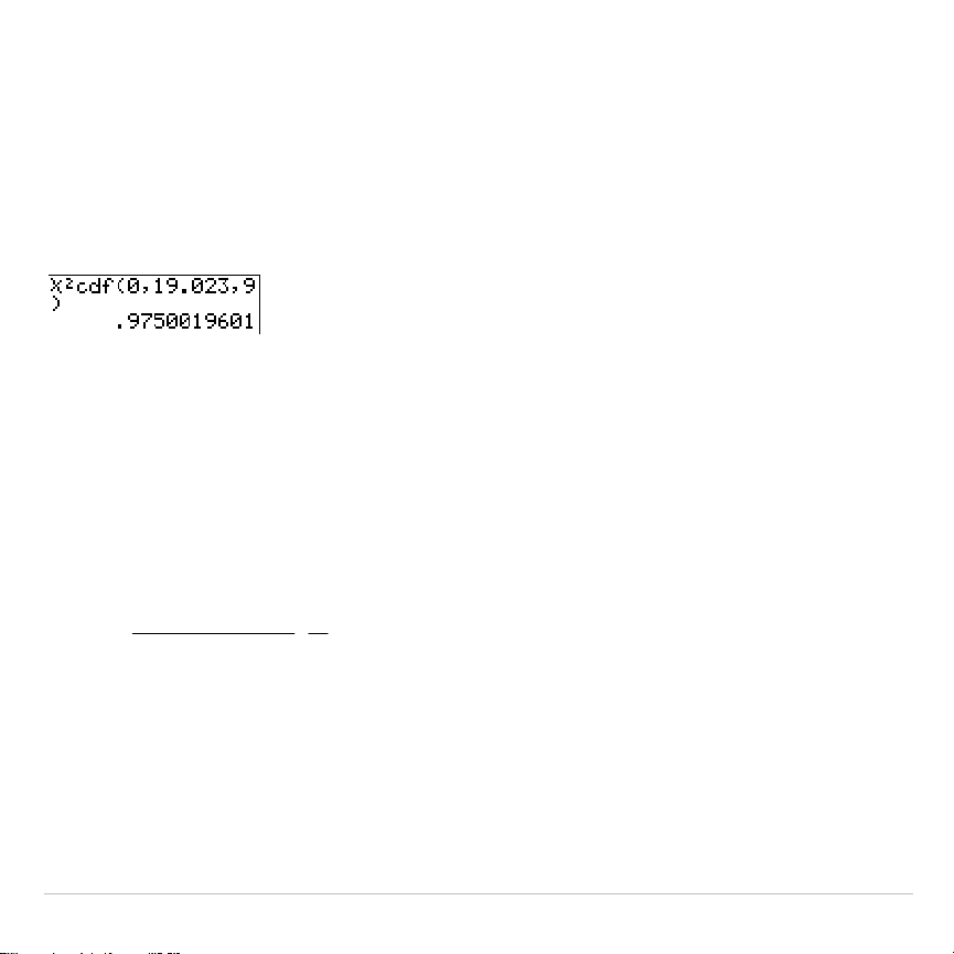
TI-83 Plus Inferential Statistics and Distributions 429
c
2
cdf(
c
2
cdf(
computes the
c
2
(chi-square) distribution probability between
lowerbound
and
upperbound
for the specified
df
(degrees of freedom), which
must be an integer > 0.
c
2
cdf(
lowerbound
,
upperbound
,
df
)
Ü
pdf(
Ü
pdf(
computes the probability density function (pdf) for the
Û
distribution
at a specified
x
value.
numerator df
(degrees of freedom) and
denominator df
must be integers > 0. To plot the
Û
distribution, paste
Ü
pdf(
to the
Y=
editor. The probability density function (pdf) is:
0,)/1(
)2/()2/(
]2/)[(
)(
2/)(12/
2/
≥+
ΓΓ
+Γ
=
+−−
xdnxx
d
n
dn
dn
xf
dnn
n
where
n
= numerator degrees of freedom
d
= denominator degrees of freedom
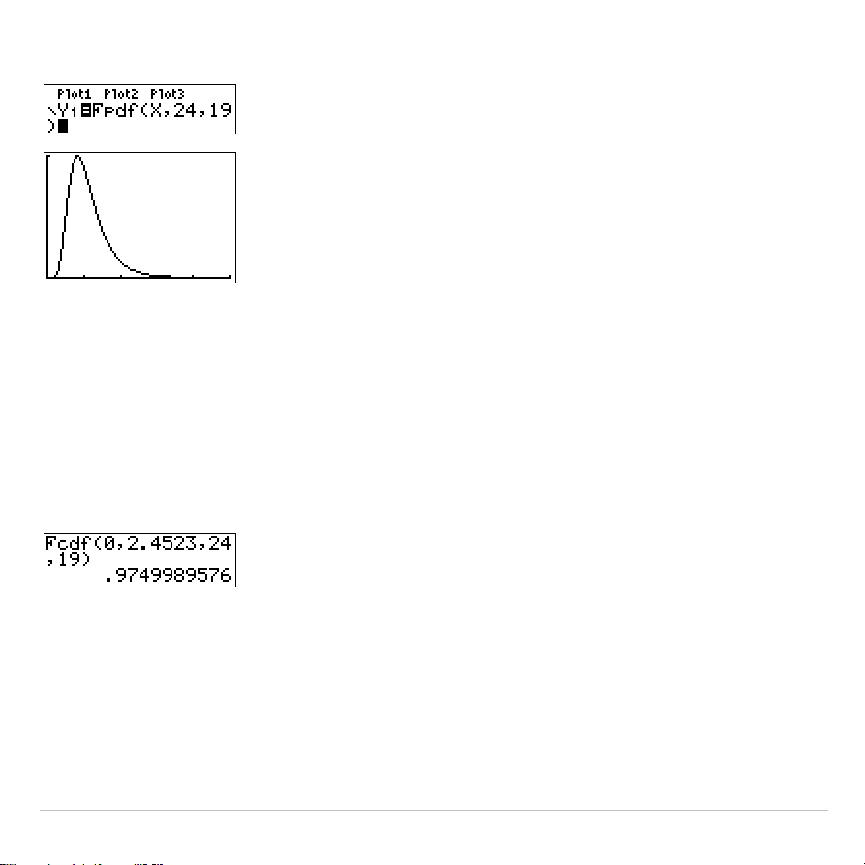
TI-83 Plus Inferential Statistics and Distributions 430
Ü
pdf(
x
,
numerator df
,
denominator df
)
Note: For this example,
Xmin = 0
Xmax = 5
Ymin = 0
Ymax = 1
Ü
cdf(
Ü
cdf(
computes the
Û
distribution probability between
lowerbound
and
upperbound
for the specified
numerator df
(degrees of freedom) and
denominator df
.
numerator df
and
denominator df
must be integers >0.
Ü
cdf(
lowerbound
,
upperbound
,
numerator df
,
denominator df
)
binompdf
binompdf(
computes a probability at
x
for the discrete binomial
distribution with the specified
numtrials
and probability of success (
p
) on
each trial.
x
can be an integer or a list of integers. 0
p
1 must be true.
numtrials
must be an integer > 0. If you do not specify
x
, a list of
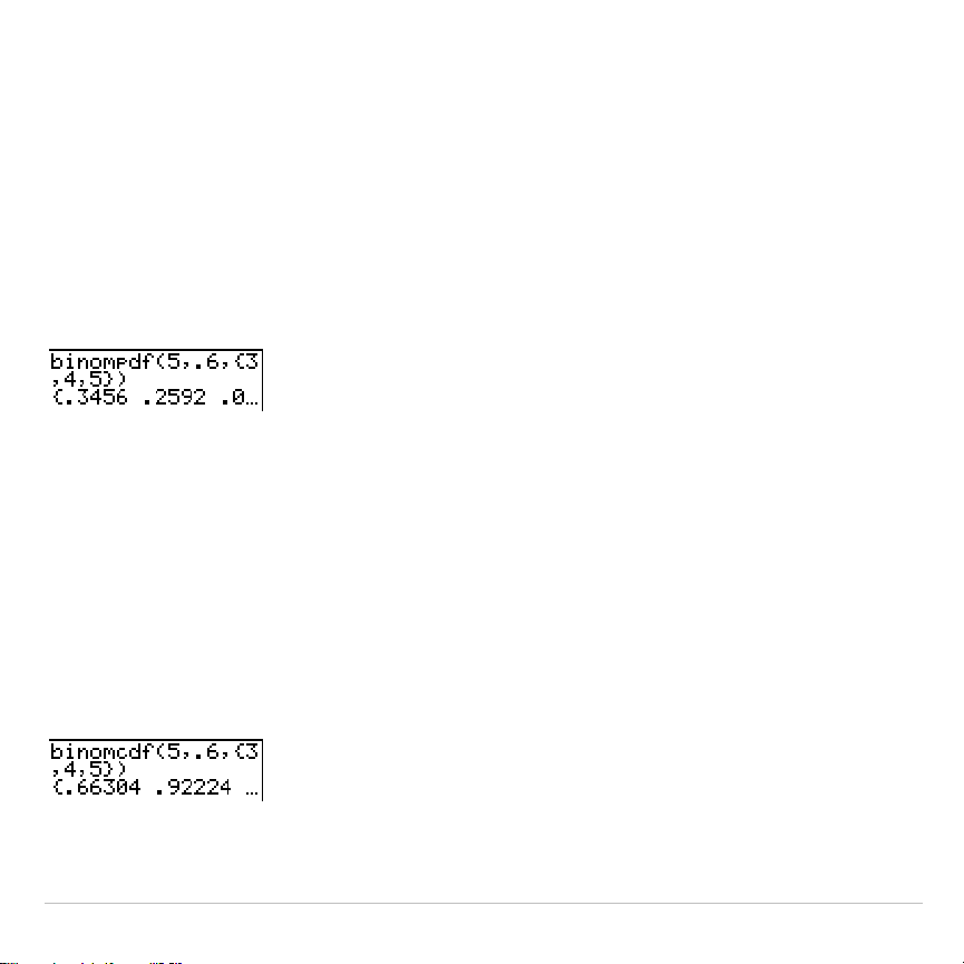
TI-83 Plus Inferential Statistics and Distributions 431
probabilities from 0 to
numtrials
is returned. The probability density
function (pdf) is:
nxpp
x
n
xf
xnx
,,1,0,)1()( K
=−
=
−
where
n = numtrials
binompdf(
numtrials
,
p
[
,
x
]
)
binomcdf(
binomcdf(
computes a cumulative probability at
x
for the discrete binomial
distribution with the specified
numtrials
and probability of success (
p
) on
each trial.
x
can be a real number or a list of real numbers. 0
p
1 must
be true.
numtrials
must be an integer > 0. If you do not specify
x
, a list of
cumulative probabilities is returned.
binomcdf(
numtrials
,
p
[
,
x
]
)
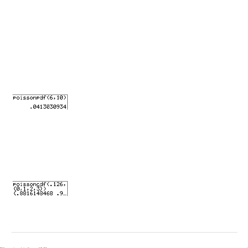
TI-83 Plus Inferential Statistics and Distributions 432
poissonpdf(
poissonpdf(
computes a probability at
x
for the discrete Poisson
distribution with the specified mean
m
, which must be a real number > 0.
x
can be an integer or a list of integers. The probability density function
(pdf) is:
,2,1,0,!/)(
==
−
xxexf
x
µ
µ
poissonpdf(
m
,
x
)
poissoncdf(
poissoncdf(
computes a cumulative probability at
x
for the discrete
Poisson distribution with the specified mean
m
, which must be a real
number > 0.
x
can be a real number or a list of real numbers.
poissoncdf(
m
,
x
)
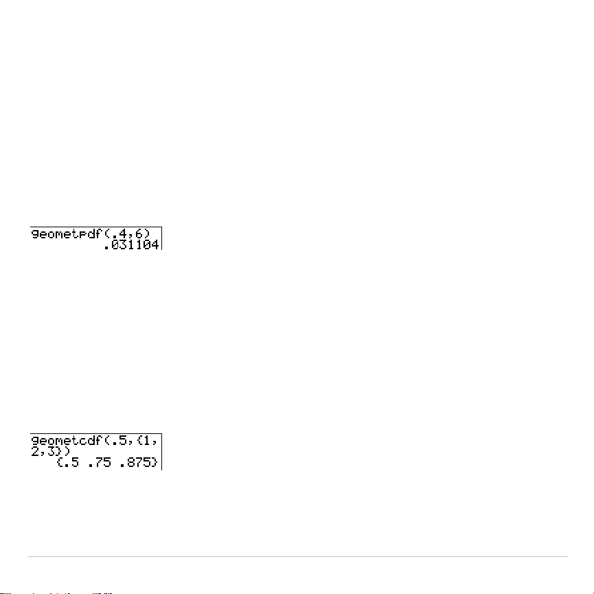
TI-83 Plus Inferential Statistics and Distributions 433
geometpdf(
geometpdf(
computes a probability at
x
, the number of the trial on which
the first success occurs, for the discrete geometric distribution with the
specified probability of success
p
. 0
p
1 must be true.
x
can be an
integer or a list of integers. The probability density function (pdf) is:
,2,1,)1()(
1
=−=
−
xppxf
x
geometpdf(
p
,
x
)
geometcdf(
geometcdf(
computes a cumulative probability at
x
, the number of the trial
on which the first success occurs, for the discrete geometric distribution
with the specified probability of success
p
. 0
p
1 must be true.
x
can be
a real number or a list of real numbers.
geometcdf(
p
,
x
)
TI-83 Plus Inferential Statistics and Distributions 434
Distribution Shading
DISTR DRAW Menu
To display the
DISTR DRAW
menu, press
y
=
~
.
DISTR DRAW
instructions draw various types of density functions, shade the area
specified by
lowerbound
and
upperbound
, and display the computed area
value.
To clear the drawings, select
1:ClrDraw
from the
DRAW
menu (Chapter 8).
Note: Before you execute a
DISTR DRAW
instruction, you must set the window
variables so that the desired distribution fits the screen.
DISTR DRAW
1: ShadeNorm(
Shades normal distribution.
2: Shade_t(
Shades Student-
t
distribution.
3: Shade
c
2
(
Shades
c
2
distribution.
4: ShadeÛ(
Shades
Û
distribution.
Note:
L
1
å
99 and 1
å
99 specify infinity. If you want to view the area left of
upperbound
, for example, specify
lowerbound
=
L
1
å
99.

TI-83 Plus Inferential Statistics and Distributions 435
ShadeNorm(
ShadeNorm(
draws the normal density function specified by mean
m
and
standard deviation
s
and shades the area between
lowerbound
and
upperbound
. The defaults are
m
=0 and
s
=1.
ShadeNorm(
lowerbound
,
upperbound
[
,
m
,
s
]
)
Note: For this example,
Xmin = 55
Xmax = 72
Ymin =
L
.05
Ymax = .2
Shade_t(
Shade_t(
draws the density function for the Student-
t
distribution specified
by
df
(degrees of freedom) and shades the area between
lowerbound
and
upperbound
.
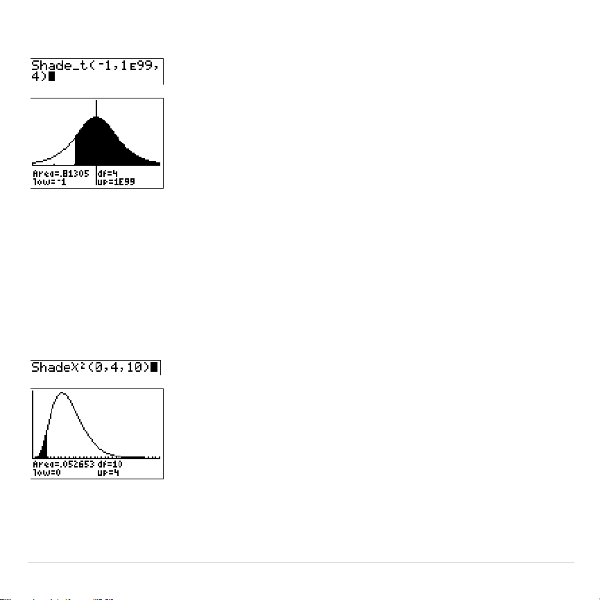
TI-83 Plus Inferential Statistics and Distributions 436
Shade_t(
lowerbound
,
upperbound
,
df
)
Note: For this example,
Xmin =
L
3
Xmax = 3
Ymin =
L
.15
Ymax = .5
Shade
c
2
(
Shade
c
2
(
draws the density function for the
c
2
(chi-square) distribution
specified by
df
(degrees of freedom) and shades the area between
lowerbound
and
upperbound
.
Shade
c
2
(
lowerbound
,
upperbound
,
df
)
Note: For this example,
Xmin = 0
Xmax = 35
Ymin =
L
.025
Ymax = .1
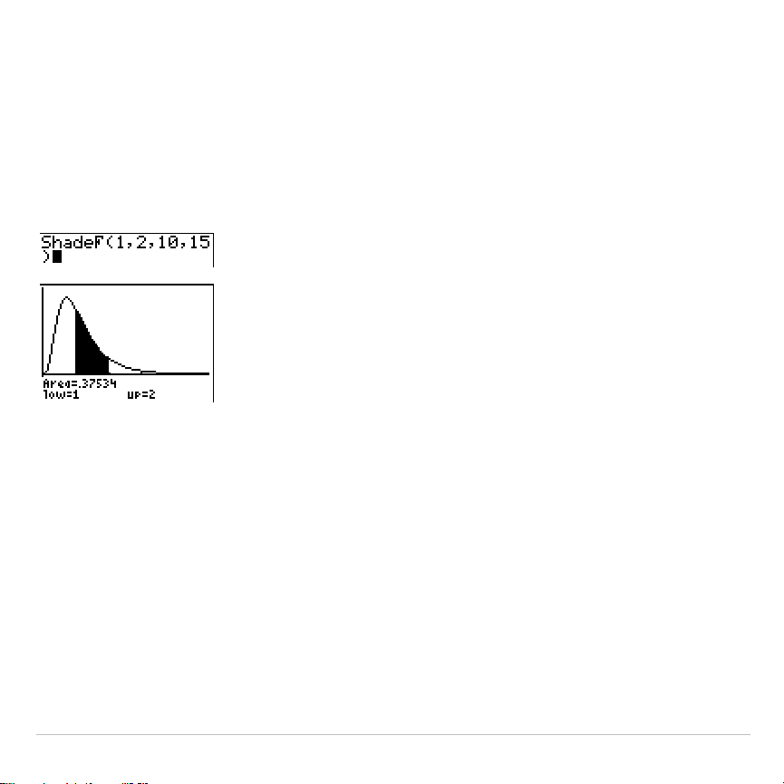
TI-83 Plus Inferential Statistics and Distributions 437
Shade
Ü
(
Shade
Ü
(
draws the density function for the
Û
distribution specified by
numerator df
(degrees of freedom)
and
denominator df
and shades the area
between
lowerbound
and
upperbound
.
Shade
Ü
(
lowerbound
,
upperbound
,
numerator df
,
denominator df
)
Note: For this example,
Xmin = 0
Xmax = 5
Ymin =
L
.25
Ymax = .9

TI-83 Plus Applications 438
Chapter 14:
Applications
The Applications Menu
The TI-83 Plus comes with
Finance
and
CBL
à
CBR
applications already
listed on the
APPLICATIONS
menu. Except for the
Finance
application, you
can add and remove applications as space permits. The
Finance
application is built into the TI-83 Plus code and cannot be deleted.
You can buy additional TI-83 Plus software applications that allow you to
customize further your calculator’s functionality. The calculator reserves
1.54 M of space within ROM memory specifically for applications.
Your TI-83 Plus includes Flash applications in addition to the ones
mentioned above. Press
Œ
to see the complete list of applications
that came with your calculator.
Documentation for TI Flash applications is on the TI Resource CD. Visit
education.ti.com/guides
for additional Flash application guidebooks.
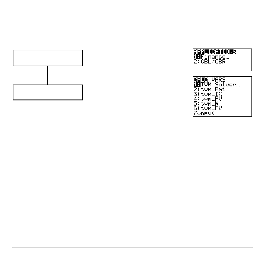
TI-83 Plus Applications 439
Steps for Running the Finance Application
Follow these basic steps when using the
Finance
application.
Select the Finance
application.
Press
9
b
.
Select from list of
functions.
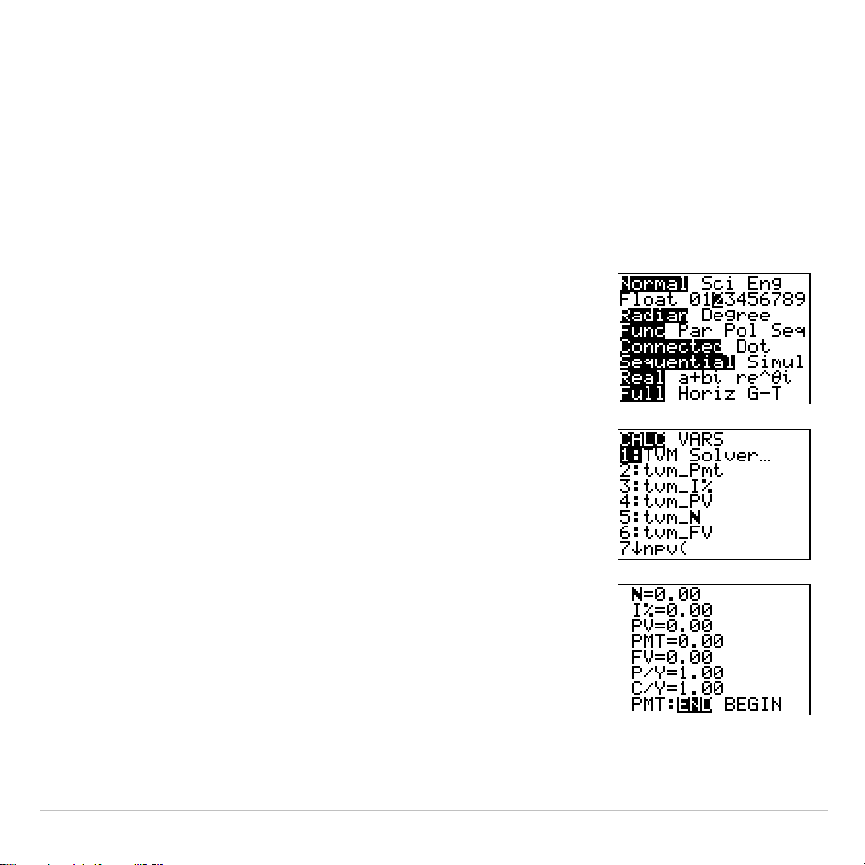
TI-83 Plus Applications 440
Getting Started: Financing a Car
Getting Started is a fast-paced introduction. Read the chapter for details.
You have found a car you would like to buy. The car costs 9,000. You can afford
payments of 250 per month for four years. What annual percentage rate (APR) will
make it possible for you to afford the car?
1. Press
z
†
~
~
~
Í
to set the fixed-
decimal mode setting to
2
. The TI-83 Plus will
display all numbers with two decimal places).
2. Press
Œ
Í
to select
1:Finance
from the
APPLICATIONS
menu.
3. Press
Í
to select
1:TVM Solver
from the
CALC VARS menu. The
TVM
Solver
is displayed.
Press
48
Í
to store 48 months to
Ú
. Press
†
9000
Í
to store 9,000 to
PV
. Press
Ì
250
Í
to store
L
250 to
PMT
. (Negation indicates
cash outflow.) Press
0
Í
to store 0 to
FV
.

TI-83 Plus Applications 441
Press
12
Í
to store 12 payments per year
to
P/Y
and 12 compounding periods per year to
C/Y
. Setting
P/Y
to 12 will compute an annual
percentage rate (compounded monthly) for
æ
.
Press
†
Í
to select
PMT:END
, which
indicates that payments are due at the end of
each period.
4. Press
}
}
}
}
}
}
to move the cursor to
the
æ
prompt. Press
ƒ
\
to solve for
æ
. What APR should you look for?
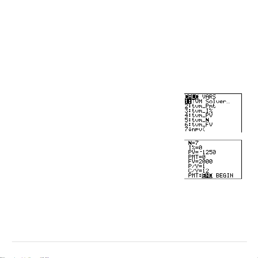
TI-83 Plus Applications 442
Getting Started: Computing Compound
Interest
At what annual interest rate, compounded monthly, will 1,250 accumulate to 2,000
in 7 years?
Note: Because there are no payments when you solve compound interest
problems,
PMT
must be set to
0
and
P/Y
must be
set to
1
.
1. Press
Œ
Í
to select
1:Finance
from the
APPLICATIONS
menu.
2. Press
Í
to select
1:TVM Solver
from the
CALC VARS
menu. The
TVM
Solver
is displayed.
Press
7
to enter the number of periods in years.
Press
†
†
Ì
1250
to enter the present value
as a cash outflow (investment). Press
†
0
to
specify no payments. Press
†
2000
to enter the
future value as a cash inflow (return). Press
†
1
to enter payment periods per year. Press
†
12
to set compounding periods per year to
12
.
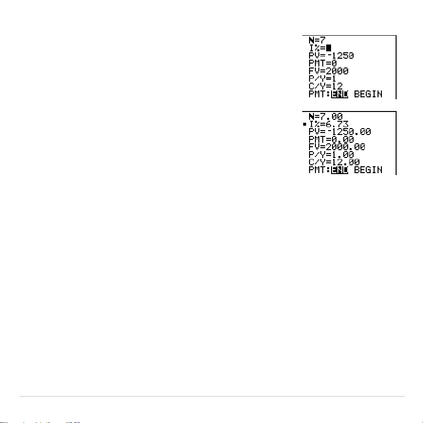
TI-83 Plus Applications 443
3. Press
}
}
}
}
}
to place the cursor on the
æ
prompt.
4. Press
ƒ
\
to solve for
æ
, the annual
interest rate.
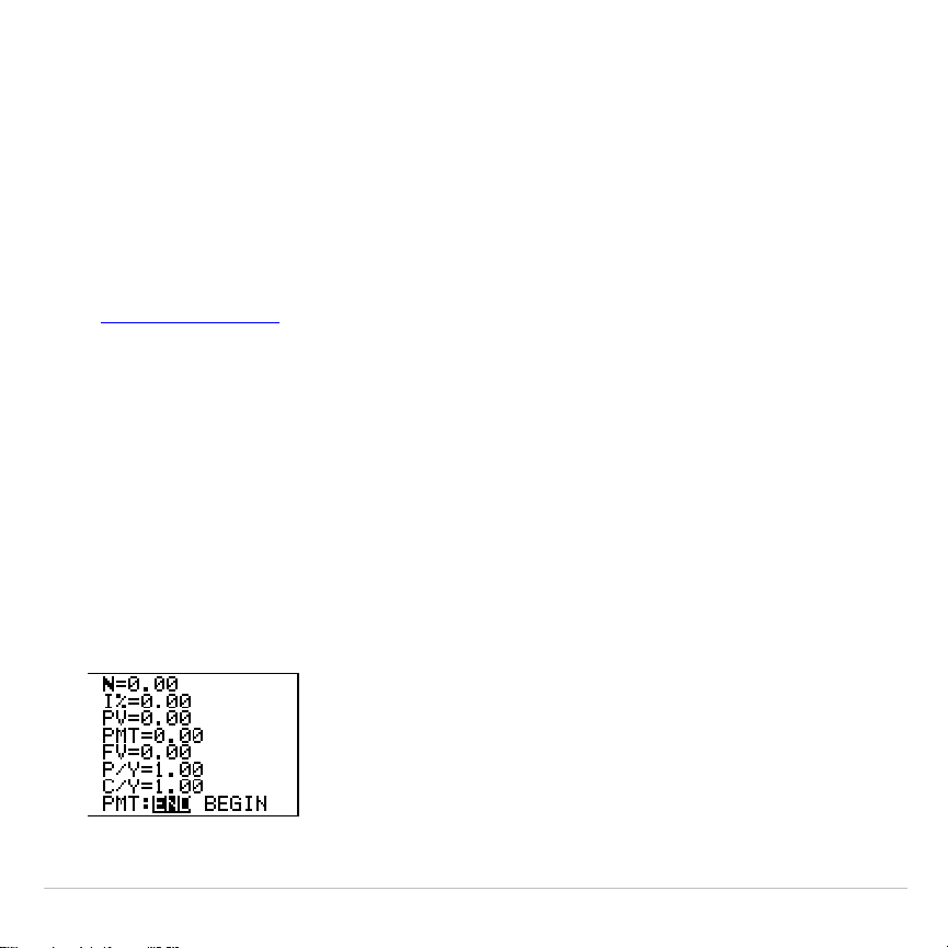
TI-83 Plus Applications 444
Using the TVM Solver
Using the TVM Solver
The
TVM Solver
displays the time-value-of-money (
TVM
) variables. Given
four variable values, the
TVM Solver
solves for the fifth variable.
The
FINANCE VARS
menu section describes the five
TVM
variables (
Ú
,
æ
,
PV
,
PMT
, and
FV
) and
P/Y
and
C/Y
.
PMT: END BEGIN
in the
TVM Solver
corresponds to the
FINANCE CALC
menu
items
Pmt_End
(payment at the end of each period) and
Pmt_Bgn
(payment at the beginning of each period).
To solve for an unknown
TVM
variable, follow these steps.
1. Press
Œ
Í
Í
to display the
TVM Solver
. The screen below
shows the default values with the fixed-decimal mode set to two
decimal places.
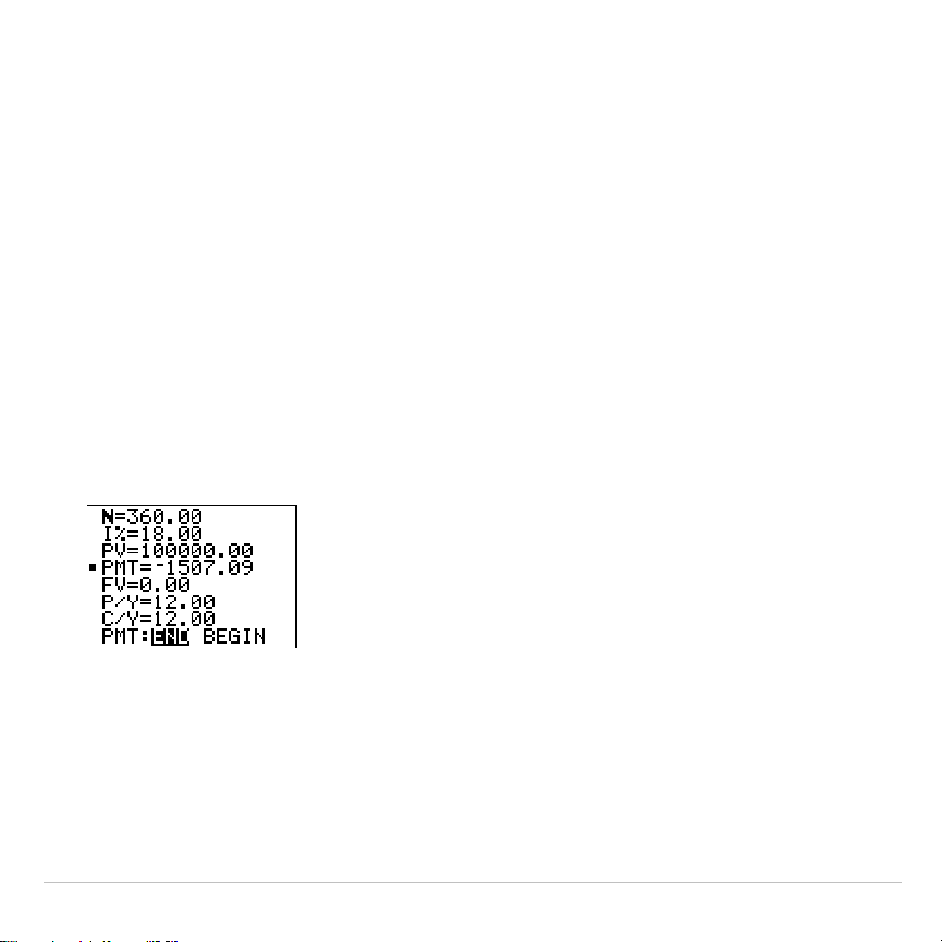
TI-83 Plus Applications 445
2. Enter the known values for four
TVM
variables.
Note: Enter cash inflows as positive numbers and cash outflows as
negative numbers.
3. Enter a value for
P/Y
, which automatically enters the same value for
C/Y
; if
P/Y
ƒ
C/Y
, enter a unique value for
C/Y
.
4. Select
END
or
BEGIN
to specify the payment method.
5. Place the cursor on the
TVM
variable for which you want to solve.
6. Press
ƒ
\
. The answer is computed, displayed in the
TVM
Solver
, and stored to the appropriate
TVM
variable. An indicator
square in the left column designates the solution variable.
TI-83 Plus Applications 446
Using the Financial Functions
Entering Cash Inflows and Cash Outflows
When using the TI-83 Plus financial functions, you must enter cash
inflows (cash received) as positive numbers and cash outflows (cash
paid) as negative numbers. The TI-83 Plus follows this convention when
computing and displaying answers.
FINANCE CALC Menu
To display the
FINANCE CALC
menu, press
Œ
Í
.
CALC VARS
1: TVM Solver
...
Displays the
TVM Solver
.
2: tvm_Pmt
Computes the amount of each payment.
3: tvm_æ
Computes the interest rate per year.
4: tvm_PV
Computes the present value.
5: tvm_Ú
Computes the number of payment periods.
6: tvm_FV
Computes the future value.
7: npv(
Computes the net present value.
8: irr(
Computes the internal rate of return.
9: bal(
Computes the amortization sched. balance.
0:
G
Prn(
Computes the amort. sched. princ. sum.
A:
G
Int(
Computes the amort. sched. interest sum.

TI-83 Plus Applications 447
CALC VARS
B:
4
Nom(
Computes the nominal interest rate.
C:
4
Eff(
Computes the effective interest rate.
D: dbd(
Calculates the days between two dates.
E: Pmt_End
Selects ordinary annuity (end of period).
F: Pmt_Bgn
Selects annuity due (beginning of period).
Use these functions to set up and perform financial calculations on the
home screen.
TVM Solver
TVM Solver
displays the
TVM Solver
.

TI-83 Plus Applications 448
Calculating Time Value of Money (TVM)
Calculating Time Value of Money
Use time-value-of-money (
TVM
) functions (menu items
2
through
6
) to
analyze financial instruments such as annuities, loans, mortgages,
leases, and savings.
Each
TVM
function takes zero to six arguments, which must be real
numbers. The values that you specify as arguments for these functions
are not stored to the
TVM
variables
.
Note: To store a value to a
TVM
variable, use the
TVM Solver
or use
¿
and
any
TVM
variable on the
FINANCE VARS
menu.
If you enter less than six arguments, the TI-83 Plus substitutes a
previously stored
TVM
variable value for each unspecified argument.
If you enter any arguments with a
TVM
function, you must place the
argument or arguments in parentheses.
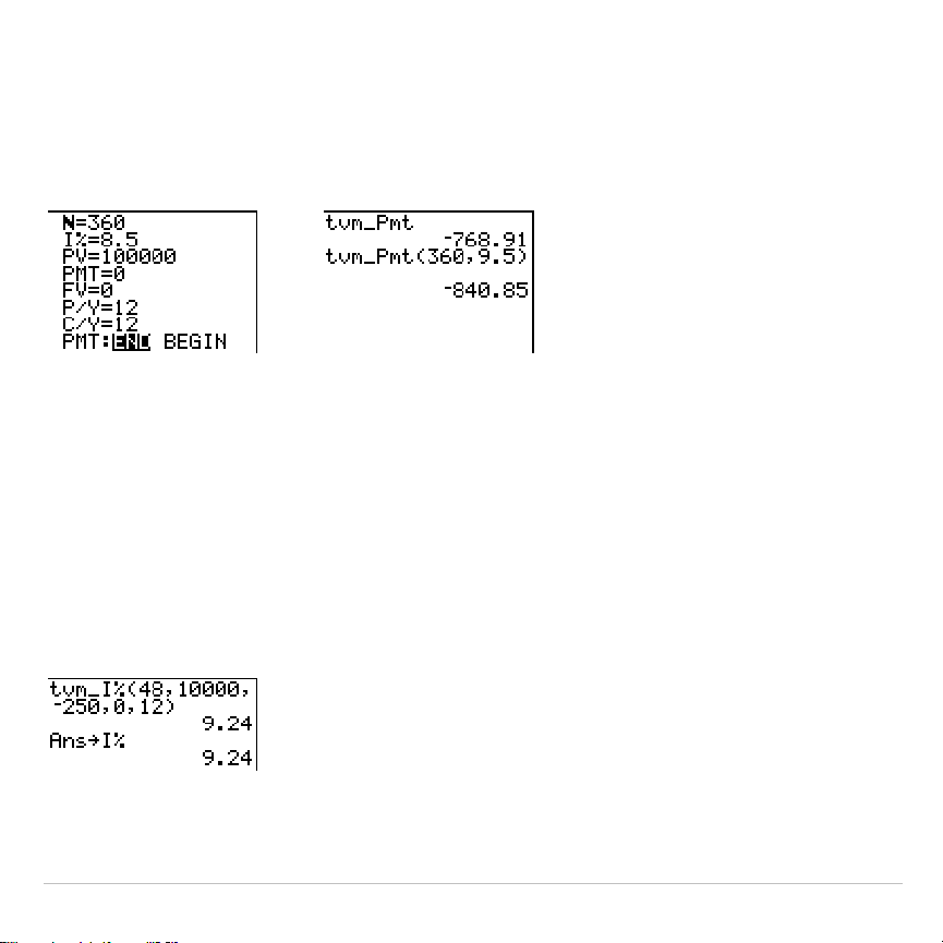
TI-83 Plus Applications 449
tvm_Pmt
tvm_Pmt
computes the amount of each payment.
tvm_Pmt
[
(
Ú
,
æ
,
PV
,
FV
,
P/Y
,
C/Y
)
]
Note: In the example above, the values are stored to the
TVM
variables in the
TVM Solver
. Then the payment (
tvm_Pmt
) is computed on the home screen
using the values in the
TVM Solver
. Next, the interest rate is changed to 9.5 to
illustrate the effect on the payment amount.
tvm_
æ
tvm_
æ
computes the annual interest rate.
tvm_
æ
[
(
Ú
,
PV
,
PMT
,
FV
,
P/Y
,
C/Y
)
]
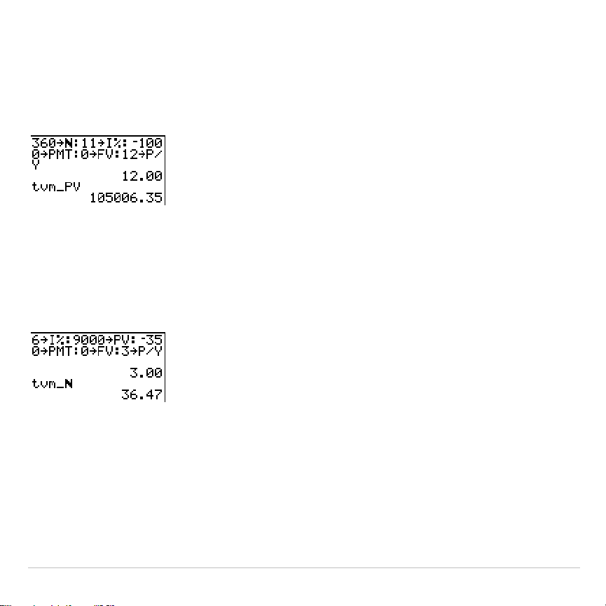
TI-83 Plus Applications 450
tvm_PV
tvm_PV
computes the present value.
tvm_PV
[
(
Ú
,
æ
,
PMT
,
FV
,
P/Y
,
C/Y
)
]
tvm_
Ú
tvm_
Ú
computes the number of payment periods.
tvm_
Ú
[
(
æ
,
PV
,
PMT
,
FV
,
P/Y
,
C/Y
)
]
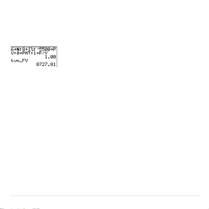
TI-83 Plus Applications 451
tvm_FV
tvm_FV
computes the future value.
tvm_FV
[
(
Ú
,
æ
,
PV
,
PMT
,
P/Y
,
C/Y
)
]
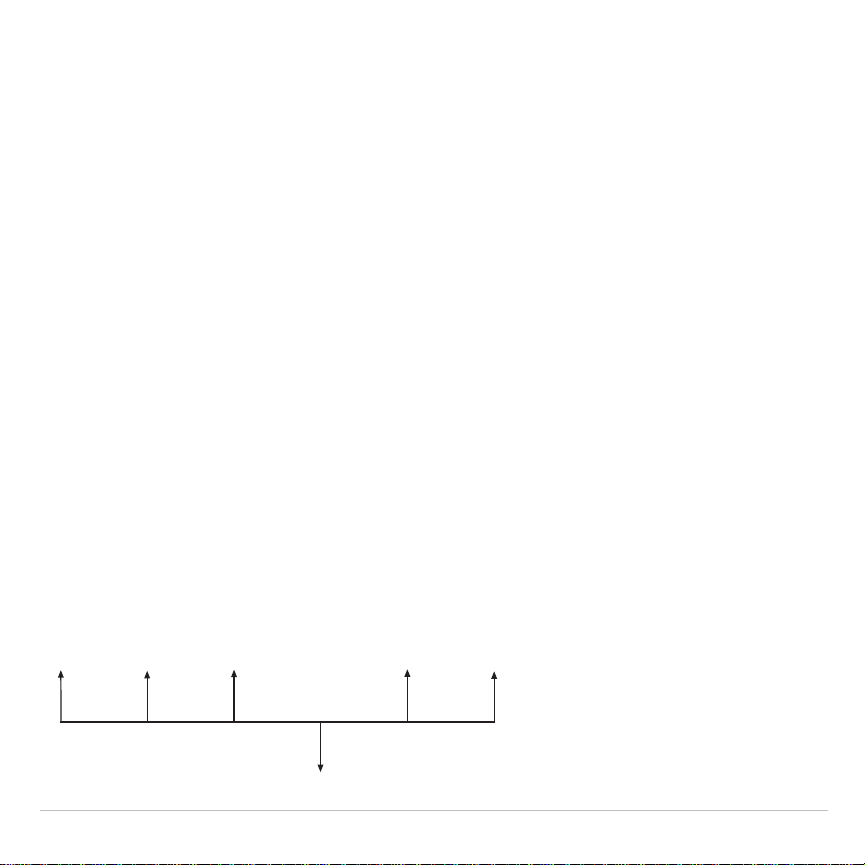
TI-83 Plus Applications 452
Calculating Cash Flows
Calculating a Cash Flow
Use the cash flow functions (menu items
7
and
8
) to analyze the value of
money over equal time periods. You can enter unequal cash flows,
which can be cash inflows or outflows. The syntax descriptions for
npv(
and
irr(
use these arguments.
•
interest rate
is the rate by which to discount the cash flows (the cost of
money) over one period.
• CF0
is the initial cash flow at time 0; it must be a real number.
•
CFList
is a list of cash flow amounts after the initial cash flow
CF0
.
•
CFFreq
is a list in which each element specifies the frequency of
occurrence for a grouped (consecutive) cash flow amount, which is
the corresponding element of
CFList
. The default is 1; if you enter
values, they must be positive integers < 10,000.
For example, express this uneven cash flow in lists.
2000
4000
2000
2000
- 3000
4000

TI-83 Plus Applications 453
CF0
=
2000
CFList
=
{2000,
L
3000,4000}
CFFreq
=
{2,1,2}
npv(, irr(
npv(
(net present value) is the sum of the present values for the cash
inflows and outflows. A positive result for
npv
indicates a profitable
investment.
npv(
interest rate
,
CF0
,
CFList
[
,
CFFreq
]
)
irr(
(internal rate of return) is the interest rate at which the net present
value of the cash flows is equal to zero.
irr(
CF0
,
CFList
[
,
CFFreq
]
)
3000
5000
1000
- 2000
- 2500
0
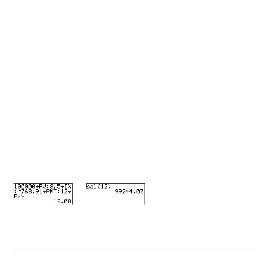
TI-83 Plus Applications 454
Calculating Amortization
Calculating an Amortization Schedule
Use the amortization functions (menu items
9
,
0
, and
A
) to calculate
balance, sum of principal, and sum of interest for an amortization
schedule.
bal(
bal(
computes the balance for an amortization schedule using stored
values for
æ
,
PV
, and
PMT
.
npmt
is the number of the payment at which
you want to calculate a balance. It must be a positive integer < 10,000.
roundvalue
specifies the internal precision the calculator uses to calculate
the balance; if you do not specify
roundvalue
, then the TI-83 Plus uses the
current
Float
/
Fix
decimal-mode setting.
bal(
npmt
[
,
roundvalue
]
)
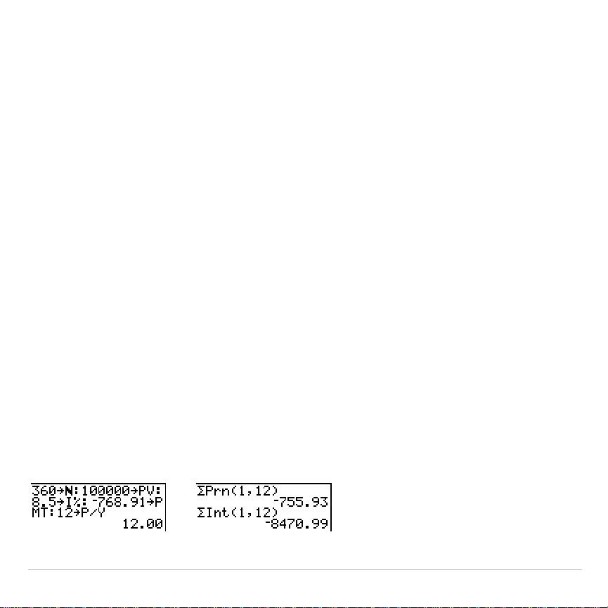
TI-83 Plus Applications 455
G
Prn(,
G
Int(
G
Prn(
computes the sum of the principal during a specified period for an
amortization schedule using stored values for
æ
,
PV
, and
PMT
.
pmt1
is the
starting payment.
pmt2
is the ending payment in the range.
pmt1
and
pmt2
must be positive integers < 10,000.
roundvalue
specifies the internal
precision the calculator uses to calculate the principal; if you do not specify
roundvalue
, the TI-83 Plus uses the current
Float
/
Fix
decimal-mode setting.
Note: You must enter values for
æ
,
PV
,
PMT
, and before computing the
principal.
G
Prn(
pmt1
,
pmt2
[
,
roundvalue
]
)
G
Int(
computes the sum of the interest during a specified period for an
amortization schedule using stored values for
æ
,
PV
, and
PMT
.
pmt1
is the
starting payment.
pmt2
is the ending payment in the range.
pmt1
and
pmt2
must be positive integers < 10,000.
roundvalue
specifies the internal
precision the calculator uses to calculate the interest; if you do not
specify
roundvalue
, the TI-83 Plus uses the current
Float
/
Fix
decimal-mode
setting.
G
Int(
pmt1
,
pmt2
[
,
roundvalue
]
)
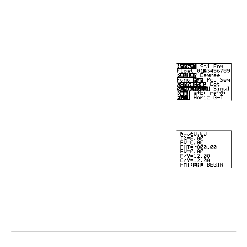
TI-83 Plus Applications 456
Amortization Example: Calculating an Outstanding Loan Balance
You want to buy a home with a 30-year mortgage at 8 percent APR.
Monthly payments are 800. Calculate the outstanding loan balance after
each payment and display the results in a graph and in the table.
1. Press
z
. Press
†
~
~
~
Í
to set the
fixed-decimal mode setting to
2
. Press
†
†
~
Í
to select
Par
graphing mode.
2.Press
Œ
Í
Í
to display the
TVM Solver
.
3. Press
Í
360
to enter number of payments.
Press
†
8
to enter the interest rate. Press
†
†
Ì
800
to enter the payment amount. Press
†
0
to enter the future value of the mortgage. Press
†
12
to enter the payments per year, which
also sets the compounding periods per year to
12
. Press
†
†
Í
to select
PMT:END
.
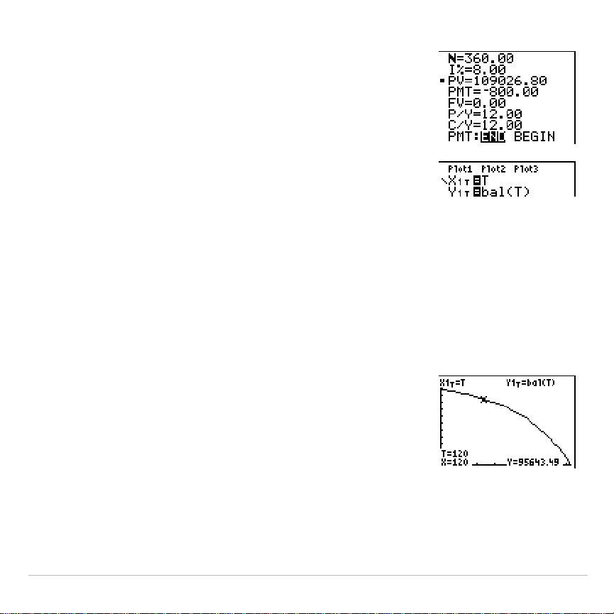
TI-83 Plus Applications 457
4. Press
}
}
}
}
}
to place the cursor on the
PV
prompt. Press
ƒ
\
to solve for the
present value.
5. Press
o
to display the parametric
Y=
editor.
Turn off all stat plots. Press
„
to define
X1T
as
T
. Press
†
Œ
Í
9
„¤
to define
Y1T
as
bal(T)
.
6. Press
p
to display the window variables.
Enter the values below.
Tmin=0 Xmin=0 Ymin=0
Tmax=360 Xmax=360 Ymax=125000
Tstep=12 Xscl=50 Yscl=10000
7. Press
r
to draw the graph and activate the
trace cursor. Press
~
and
|
to explore the
graph of the outstanding balance over time.
Press a number and then press
Í
to view
the balance at a specific time
T
.
8. Press
y
-
and enter the values below.
TblStart=0
@
Tbl=12
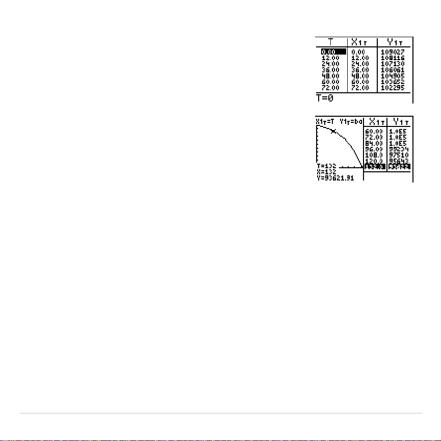
TI-83 Plus Applications 458
9. Press
y
0
to display the table of
outstanding balances (
Y1T
).
10.Press
z
†
†
†
†
†
†
†
~
~
Í
to
select
G
.
T
split-screen mode, in which the
graph and table are displayed simultaneously.
Press
r
to display
X1T
(time) and
Y1T
(balance) in the table.
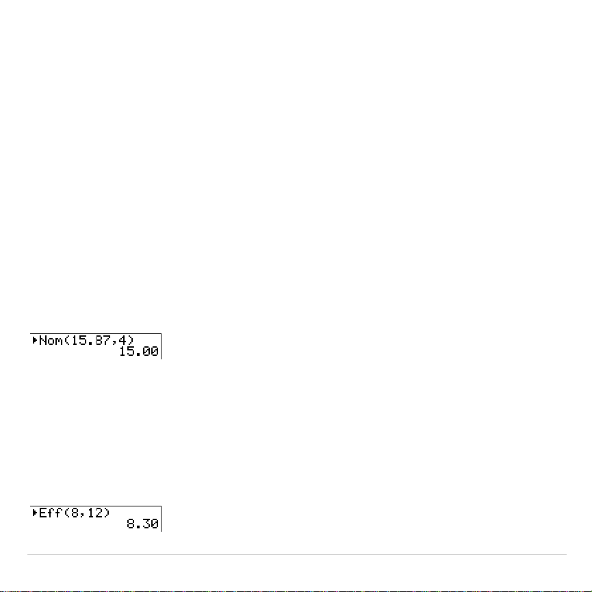
TI-83 Plus Applications 459
Calculating Interest Conversion
Calculating an Interest Conversion
Use the interest conversion functions (menu items
B
and
C
) to convert
interest rates from an annual effective rate to a nominal rate (
4
Nom(
) or
from a nominal rate to an annual effective rate (
4
Eff(
).
4
Nom(
4
Nom(
computes the nominal interest rate.
effective rate
and
compounding
periods
must be real numbers.
compounding periods
must be >0.
4
Nom(
effective rate
,
compounding periods
)
4
Eff(
4
Eff(
computes the effective interest rate.
nominal rate
and
compounding
periods
must be real numbers.
compounding periods
must be >0.
4
Eff(
nominal rate
,
compounding periods
)
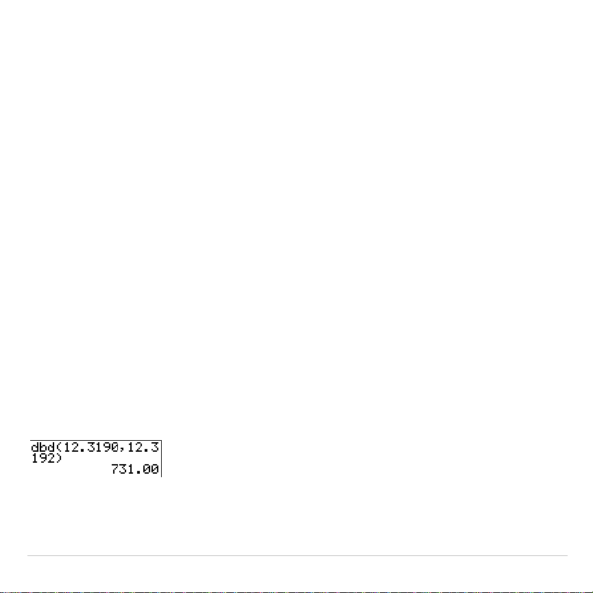
TI-83 Plus Applications 460
Finding Days between Dates/Defining
Payment Method
dbd(
Use the date function
dbd(
(menu item
D
) to calculate the number of days
between two dates using the actual-day-count method.
date1
and
date2
can be numbers or lists of numbers within the range of the dates on the
standard calendar.
Note: Dates must be between the years 1950 through 2049.
dbd(
date1
,
date2
)
You can enter
date1
and
date2
in either of two formats.
•
MM.DDYY (United States)
•
DDMM.YY (Europe)
The decimal placement differentiates the date formats.

TI-83 Plus Applications 461
Defining the Payment Method
Pmt_End
and
Pmt_Bgn
(menu items
E
and
F
) specify a transaction as an
ordinary annuity or an annuity due. When you execute either command,
the
TVM Solver
is updated.
Pmt_End
Pmt_End
(payment end) specifies an ordinary annuity, where payments
occur at the end of each payment period. Most loans are in this category.
Pmt_End
is the default.
Pmt_End
On the
TVM Solver
’s
PMT:END BEGIN
line, select
END
to set
PMT
to
ordinary annuity.
Pmt_Bgn
Pmt_Bgn
(payment beginning) specifies an annuity due, where payments
occur at the beginning of each payment period. Most leases are in this
category.
Pmt_Bgn
On the
TVM Solver
’s
PMT:END BEGIN
line, select
BEGIN
to set
PMT
to
annuity due.
TI-83 Plus Applications 462
Using the TVM Variables
FINANCE VARS Menu
To display the
FINANCE VARS
menu, press
Œ
Í
~
. You can use
TVM
variables in
TVM
functions and store values to them on the home
screen.
CALC VARS
1:Ú
Total number of payment periods
2:æ
Annual interest rate
3:PV
Present value
4:PMT
Payment amount
5:FV
Future value
6:P/Y
Number of payment periods per year
7:C/Y
Number of compounding periods/year
Ú
,
æ
, PV, PMT, FV
Ú
,
æ
,
PV
,
PMT
, and
FV
are the five
TVM
variables. They represent the
elements of common financial transactions, as described in the table
above.
æ
is an annual interest rate that is converted to a per-period rate
based on the values of
P/Y
and
C/Y
.

TI-83 Plus Applications 463
P/Y and C/Y
P/Y
is the number of payment periods per year in a financial transaction.
C/Y
is the number of compounding periods per year in the same
transaction.
When you store a value to
P/Y
, the value for
C/Y
automatically changes
to the same value. To store a unique value to
C/Y
, you must store the
value to
C/Y
after you have stored a value to
P/Y
.
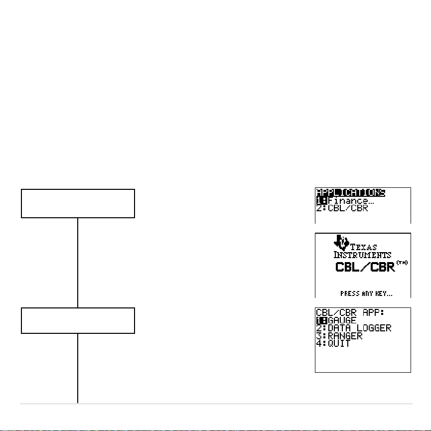
TI-83 Plus Applications 464
The CBL/CBR Application
The
CBL/CBR
application allows you to collect real world data. The
TI-83 Plus comes with the
CBL
à
CBR
application already listed on the
APPLICATIONS
menu (
9
2
).
Steps for Running the CBL
à
CBR Application
Follow these basic steps when using the
CBL
à
CBR
application. You may
not have to do all of them each time.
Select the CBL
à
CBR
application.
Press
9
2
.
Specify the data collection
method.
Press 1, 2, or 3
.
Press
b
.
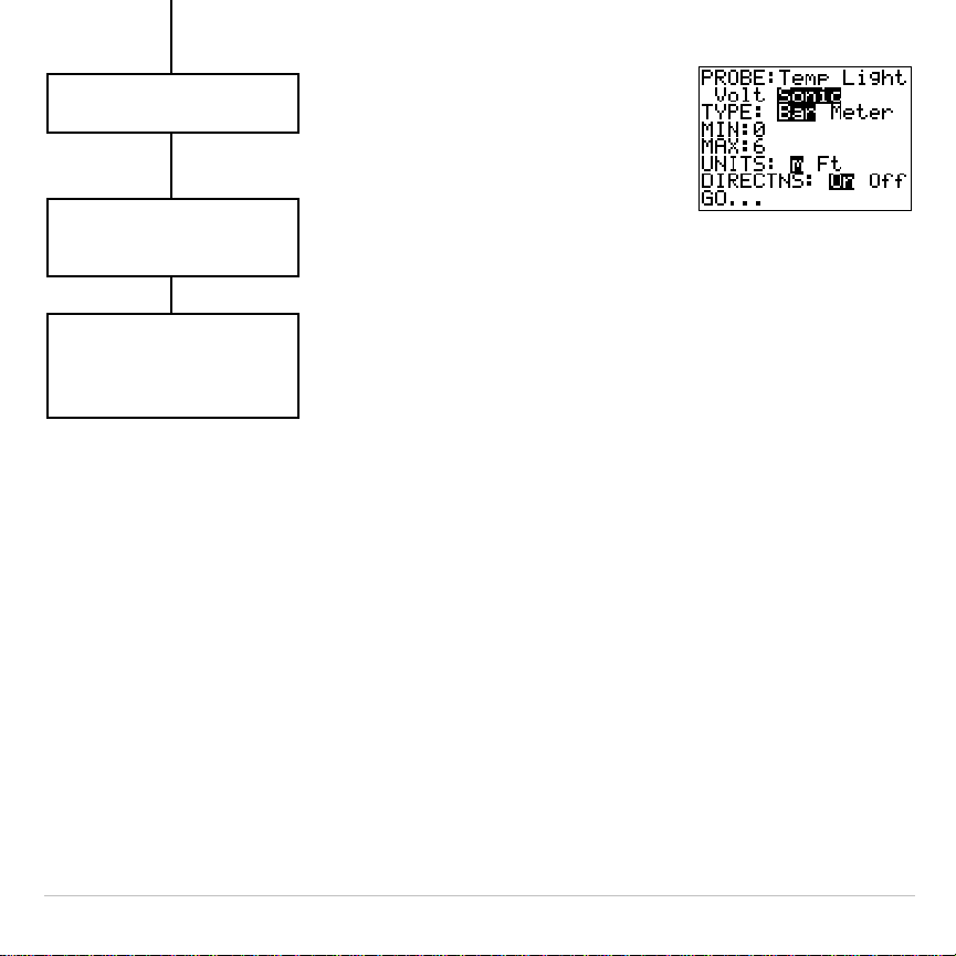
TI-83 Plus Applications 465
Select options, if
applicable.
Collect the data.
Follow directions, if
applicable.
Select
Go…
or
START NOW
.
Stop the data collection, if
necessary. Repeat these
steps or exit the
APPLICATIONS menu.
Press
^
and
° or ±.
Highlight options
or enter value and
press
b
.
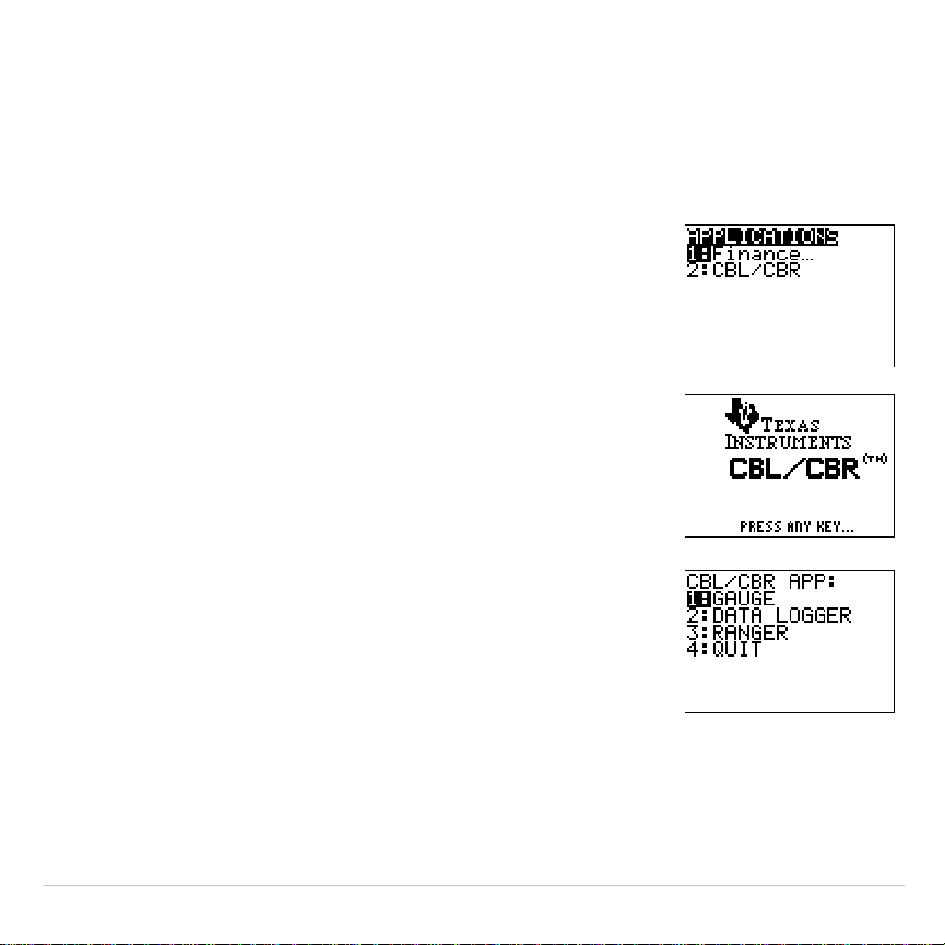
TI-83 Plus Applications 466
Selecting the CBL/CBR Application
To use a
CBL/CBR
application, you need a
CBL 2/CBL
or
CBR
(as
applicable), a TI-83 Plus, and a unit-to-unit link cable.
1. Press
Œ
.
2. Select
2:CBL/CBR
to set up the TI-83 Plus to
use either of the applications. An informational
screen appears first.
3. Press any key to continue to the next menu.

TI-83 Plus Applications 467
Data Collection Methods and Options
Specifying the Data Collection Method from the CBL/CBR APP
Menu
With a
CBL 2/CBL
or
CBR
, you can collect data in one of three ways:
GAUGE
(bar or meter),
DATA LOGGER
(a Temp-Time, Light-Time, Volt-Time, or
Sonic-Time graph), or
RANGER
, which runs the
RANGER
program, the
built-in
CBR
data collection program.
The
CBL/CBR APP
menu contains the following data collection methods:
CBL/CBR APP:
1: GAUGE
Displays results as either a bar or meter.
2: DATA LOGGER
Displays results as a Temp-Time, Light-Time, Volt-Time, or
Sonic-Time graph.
3: RANGER
Sets up and runs the
RANGER
program.
4: QUIT
Quits the CBL
à
CBR application.
Note:
CBL 2/CBL
and
CBR
differ in that
CBL 2/CBL
allows you to collect data using
one of several different probes including: Temp (Temperature), Light, Volt
(Voltage), or Sonic. CBR collects data using only the built-in Sonic probe. You
can find more information on CBL 2/CBL and CBR in their user manuals.
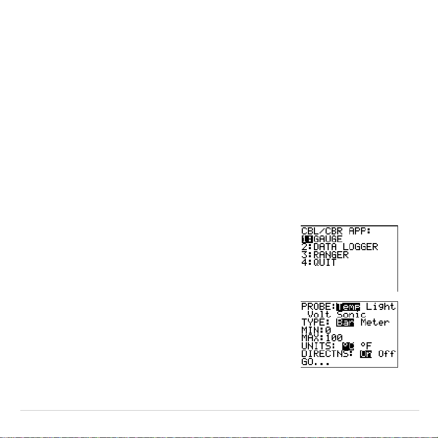
TI-83 Plus Applications 468
Specifying Options for Each Data Collection Method
After you select a data collection method from the
CBL/CBR APP
menu, a
screen showing the options for that method is displayed. The method
you choose, as well as the data collection options you choose for that
method, determine whether you use the
CBR
or the
CBL 2/CBL
. Refer to
the charts in the following sections to find the options for the application
you are using.
GAUGE
The
GAUGE
data collection method lets you choose one of four different
probes: temp, Light, Volt, or Sonic.
1. Press
Œ
2
Í
.
2. Select
1:GAUGE
.
3. Select options.
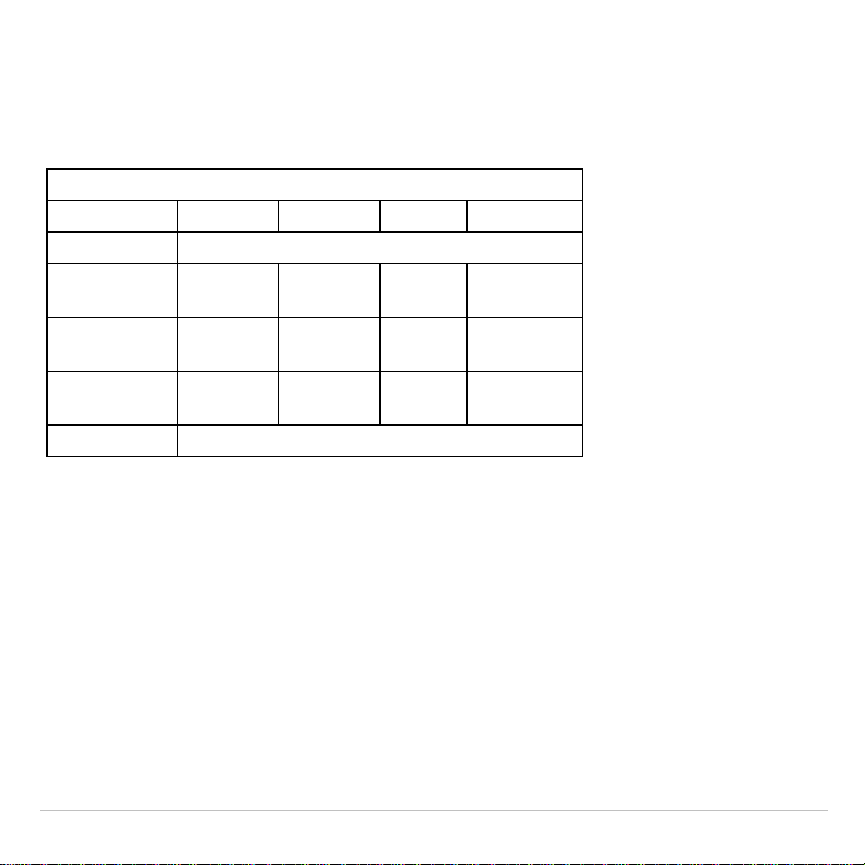
TI-83 Plus Applications 469
When you select a probe option, all other options change accordingly.
Use
"
and
!
to move between the probe options. To select a probe,
highlight the one you want with the cursor keys, and then press
Í
.
GAUGE Options (Defaults)
Probe:
Temp Light Volt Sonic
Type: Bar or Meter
Min:
00
M
10 0
Max:
100 1 10 6
Units:
¡
C or
¡
FmW
à
cm
2
Volt m or Ft
Directions: On or Off
TYPE
The
GAUGE
data collection results are represented according to
TYPE
:
Bar
or
Meter
. Highlight the one you want with the cursor keys, and then press
Í
.
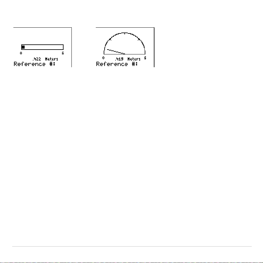
TI-83 Plus Applications 470
Bar Meter
MIN and MAX
MIN
and
MAX
refer to the minimum and maximum
UNIT
values for the
specified probe. Defaults are listed in the Gauge Options table. See the
CBL 2/CBL and CBR guidebook for specific
MIN
à
MAX
ranges. Enter
values using the number keys.
UNITS
The results are displayed according to the
UNITS
specified. To specify a
unit measurement (
Temp
or
Sonic
probes only), highlight the one you
want using the cursor keys, enter a value using the number keys, and
then press
Í
.

TI-83 Plus Applications 471
DIRECTNS (Directions)
If
DIRECTNS=On
, the calculator displays step-by-step directions on the
screen, which help you set up and run the data collection. To select
On
or
Off
, highlight the one you want with the cursor keys, and then press
Í
.
With the
Sonic
data collection probe, if
DIRECTNS=On
, the calculator
displays a menu screen before starting the application asking you to
select
1:CBL
or
2:CBR.
This ensures that you get the appropriate
directions. Press
1
to specify
CBL 2/CBL
or
2
to specify
CBR
.
Data Collection Comments and Results
To label a specific data point, press
Í
to pause the data collection.
You will see a
Reference#:
prompt. Enter a number using the number
keys. The calculator automatically converts the reference numbers and
the corresponding results into list elements using the following list names
(you cannot rename these lists):
Probe Comment Labels (
X
) Stored to: Data Results (
Y
) Stored to:
Temp
Ù
TREF
Ù
TEMP
Light
ÙLREF ÙLIGHT
Volt
ÙVREF ÙVOLT
Sonic
ÙDREF ÙDIST

TI-83 Plus Applications 472
To see all elements in one of these lists, you can insert these lists into
the List editor just as you would any other list. Access list names from
the
-
9
NAMES
menu.
Note: These lists are only temporary placeholders for comment labels and data
results for any particular probe. Therefore, every time you collect data and enter
comments for one of the four probes, the two lists pertaining to that probe are
overwritten with comment labels and data results from the most recently
collected data..
If you want to save comment labels and data results from more than one
data collection, copy all list elements that you want to save to a list with a
different name.
Also, the
DATA LOGGER
data collection method stores data results to the
same list names, overwriting previously-collected data results, even
those collected using the
GAUGE
data collection method.
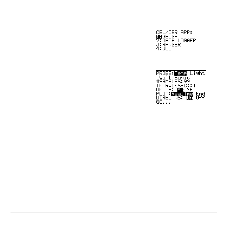
TI-83 Plus Applications 473
DATA LOGGER
1. Press
Œ
2
Í
.
2. Select
2:DATA LOGGER
.
The
DATA LOGGER
data collection method lets you choose one of four
different probes:
Temp
,
Light
,
Volt
, or
Sonic
. You can use the
CBL 2/CBL
with all probes; you can use the
CBR
only with the
Sonic
probe.
When you select a probe option, all other options change accordingly.
Use
"
and
!
to move between the probe options. To select a probe,
highlight the one you want with the cursor keys, and then press
Í
.
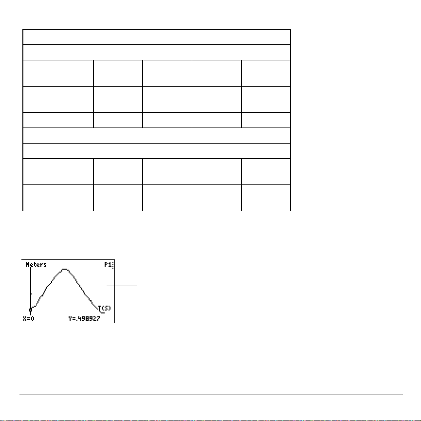
TI-83 Plus Applications 474
DATA LOGGER Options (Defaults)
Temp Light Volt Sonic
#SAMPLES:
99 99 99 99
INTRVL
(SEC):
1111
UNITS:
¡
C or
¡
F mW/cm
2
Volt Cm or Ft
PLOT: RealTme or End
DIRECTNS: On or Off
Ymin
(
'
):
00
M
10 0
Ymax
(
'
):
100 1 10 6
The
DATA LOGGER
data collection results are represented as a
Temp-Time, Light-Time, Volt-Time, or Distance-Time graph.
A Distance-Time graph in
meters (
Sonic
probe).

TI-83 Plus Applications 475
#SAMPLES
#SAMPLES
refers to how many data samples are collected and then
graphed. For example, if
#SAMPLES=99
, data collection stops after the
99
th
sample is collected. Enter values using the number keys.
INTRVL (SEC)
INTRVL
(SEC)
specifies the interval in seconds between each data sample
that is collected. For example, if you want to collect 99 samples and
INTRVL=1
, it takes 99 seconds to finish data collection. Enter values using
the number keys. See the
CBL 2/CBL
or
CBR
guidebook for more
information about interval limits.
UNITS
The results are displayed according to the
UNITS
specified. To specify a
unit measurement (
Temp
or
Sonic
only), highlight the one you want using
the cursor keys, and then press
Í
.

TI-83 Plus Applications 476
PLOT
You can specify whether you want the calculator to collect realtime
(
RealTme
) samples, which means that the calculator graphs data points
immediately as they are being collected, or you can wait and show the
graph only after all data points have been collected (
End
). Highlight the
option you want with the cursor keys, and then press
Í
.
Ymin and Ymax
To specify
Ymin
and
Ymax
values for the final graph, press
p
to view
the
PLOT WINDOW
screen. Use
$
and
#
to move between options. Enter
Ymin
and
Ymax
using the number keys. Press
-
l
to return to the
DATA LOGGER
options screen.
DIRECTNS (Directions)
If
DIRECTNS=On
, the calculator displays step-by-step directions on the
screen, which help you set up and run the data collection. To select
On
or
Off
, highlight the one you want with the cursor keys, and then press
b
.
With the
Sonic
data collection probe, if
DIRECTNS=On
, the calculator
displays a menu screen before starting the application asking you to
select
1:CBL
or
2:CBR.
This ensures that you get the appropriate
directions. Press
1
to specify
CBL 2/CBL
or
2
to specify
CBR
.

TI-83 Plus Applications 477
Data Collection Results
The calculator automatically converts all collected data points into list
elements using the following list names (you cannot rename the lists):
Probe Time Values (
X
) stored to: Data Results (
Y
) Stored to:
Temp
¨
TTEMP
¨
TEMP
Light
¨
TLGHT
¨
LIGHT
Volt
¨
TVOLT
¨
VOLT
Sonic
¨
TDIST
¨
DIST
To see all elements in one of these lists, you can insert these lists into
the List editor just as you would any other list. Access list names from
the
-
9
NAMES
menu.
Note: These lists are only temporary placeholders for data results for any
particular probe. Therefore, every time you collect data for one of the four
probes, the list pertaining to that probe is overwritten with data results from the
most recently collected data.
If you want to save data results from more than one data collection, copy
all list elements that you want to save to a list with a different name.
Also, the
GAUGE
data collection method stores data results to the same
list names, overwriting previously-collected data results, even those
collected using the
DATA LOGGER
data collection method.
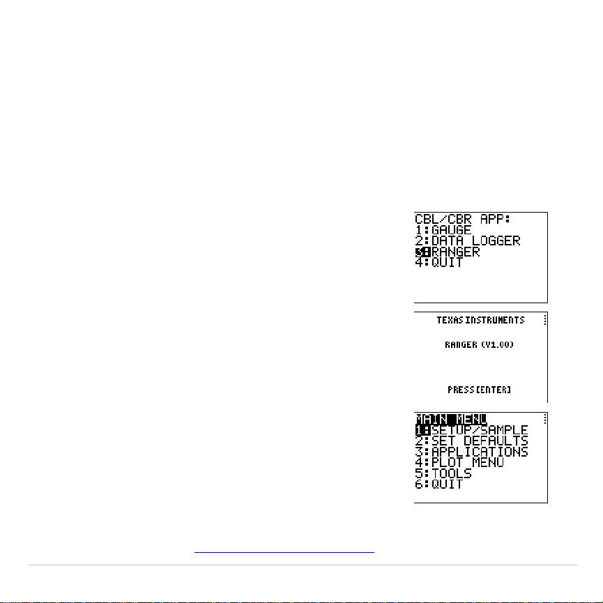
TI-83 Plus Applications 478
RANGER
Selecting the
RANGER
data collection method runs the CBR
RANGER
program, a customized program especially for the TI-83 Plus that makes
it compatible with the CBR. When the collection process is halted, the
CBR RANGER
is deleted from RAM. To run the CBR
RANGER
program
again, press
Œ
and select the
CBL/CBR
application.
Note: The Ranger data collection method only uses the Sonic probe.
1. Press
9
2
b
.
2. Select
3:RANGER
.
3. Press
b
.
4. Select options.
For detailed information about the
RANGER
program as well as option
explanations, see the
Getting Started with CBR
guidebook.

TI-83 Plus Applications 479
Starting Data Collection
Collecting the Data
After you specify all of the options for your data collection method, select
the
Go
option from the
GAUGE
or
DATA LOGGER
options screen. If you are
using the
RANGER
data collection method, select
1:SETUP
à
SAMPLE
from the
MAIN
menu, and then
START NOW
.
•
If
DIRECTNS=Off
,
GAUGE
and
DATA LOGGER
data collection begin
immediately.
•
If
DIRECTNS=On
, the calculator displays step-by-step directions.
If
PROBE=Sonic
, the calculator first displays a menu screen asking you to
select
1:CBL
or
2:CBR.
This ensures that you get the appropriate
directions. Press
1
to specify
CBL 2/CBL
or
2
to specify
CBR
.
If you select
START NOW
from the
MAIN menu
of the
RANGER
data
collection method, the calculator displays one directions screen. Press
b
to begin data collection.

TI-83 Plus Applications 480
Stopping Data Collection
To stop the
GAUGE
data collection method, press
:
on the
TI-83 Plus.
The
DATA LOGGER
and
RANGER
data collection methods stop after the
specified number of samples have been collected. To stop them before
this happens:
1. Press
^
on the TI-83 Plus.
2.Press
¤
on the CBR,
T
on the CBL 2, or
P
on the
CBL.
To exit from the
GAUGE
or
DATA LOGGER
option menus without beginning
data collection, press
-
l
.
To exit from the
RANGER
option menu without beginning data collection,
select
MAIN
menu. Select
6:QUIT
to return to the
CBL
à
CBR APP
menu.
Press
4:QUIT
from the
CBL
à
CBR APP
menu to return to the TI-83 Plus
Home screen.

TI-83 Plus CATALOG, Strings, Hyperbolic Functions 481
Chapter 15:
CATALOG, Strings, Hyperbolic
Functions
Browsing the TI-83 Plus CATALOG
What Is the CATALOG?
The
CATALOG
is an alphabetical list of all functions and instructions on the
TI
-
83 Plus. You also can access each
CATALOG
item from a menu or the
keyboard, except:
•
The six string functions
•
The six hyperbolic functions
•
The
solve(
instruction without the equation solver editor (Chapter 2)
•
The inferential stat functions without the inferential stat editors
(Chapter 13)
Note: The only
CATALOG
programming commands you can execute from the
home screen are
GetCalc(
,
Get(
, and
Send(
.
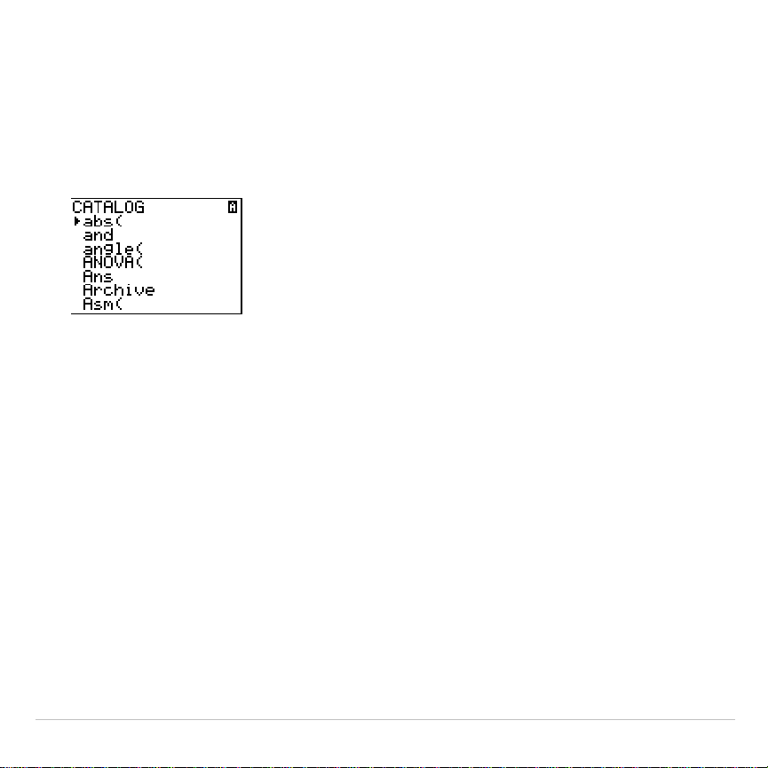
TI-83 Plus CATALOG, Strings, Hyperbolic Functions 482
Selecting an Item from the CATALOG
To select a
CATALOG
item, follow these steps.
1. Press
y
ã
CATALOGä
to display the
CATALOG
.
The
4
in the first column is the selection cursor.
2. Press
†
or
}
to scroll the
CATALOG
until the selection cursor points to
the item you want.
•
To jump to the first item beginning with a particular letter, press
that letter; alpha-lock is on.
•
Items that begin with a number are in alphabetical order according
to the first letter after the number. For example,
2
.
PropZTest(
is
among the items that begin with the letter
P
.
•
Functions that appear as symbols, such as
+
,
L
1
,
<
, and
‡
(
, follow
the last item that begins with
Z
. To jump to the first symbol,
!
,
press [
q
].
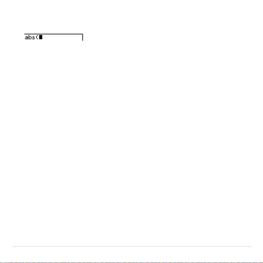
TI-83 Plus CATALOG, Strings, Hyperbolic Functions 483
3. Press
Í
to paste the item to the current screen.
Tip:
From the top of the
CATALOG
menu, press
}
to move to the bottom. From
the bottom, press
†
to move to the top.

TI-83 PlusCATALOG, Strings, Hyperbolic Functions484
Entering and Using Strings
What Is a String?
A string is a sequence of characters that you enclose within quotation
marks. On the TI-83 Plus, a string has two primary applications.
•
It defines text to be displayed in a program.
•
It accepts input from the keyboard in a program.
Characters are the units that you combine to form a string.
•
Count each number, letter, and space as one character.
•
Count each instruction or function name, such as
sin(
or
cos(
, as one
character; the TI
-
83 Plus interprets each instruction or function name
as one character.
Entering a String
To enter a string on a blank line on the home screen or in a program,
follow these steps.
1. Press
ƒ
[
ã
] to indicate the beginning of the string.
2. Enter the characters that comprise the string.
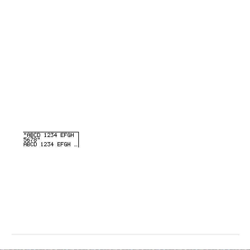
TI-83 Plus CATALOG, Strings, Hyperbolic Functions 485
•
Use any combination of numbers, letters, function names, or
instruction names to create the string.
•
To enter a blank space, press
ƒ
[
'
].
•
To enter several alpha characters in a row, press
y
7
to
activate alpha-lock.
3. Press
ƒ
[
ã
] to indicate the end of the string.
"
string
"
4. Press
Í
. On the home screen, the string is displayed on the next
line without quotations. An ellipsis (
...
) indicates that the string continues
beyond the screen. To scroll the entire string, press
~
and
|
.
Note: Quotation marks do not count as string characters.
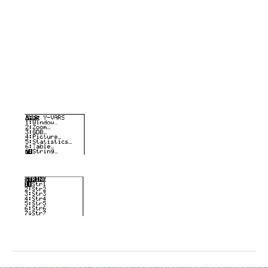
TI-83 PlusCATALOG, Strings, Hyperbolic Functions486
Storing Strings to String Variables
String Variables
The TI-83 Plus has 10 variables to which you can store strings. You can
use string variables with string functions and instructions.
To display the
VARS STRING
menu, follow these steps.
1. Press
to display the
VARS
menu. Move the cursor to
7:String
.
2. Press
Í
to display the
STRING
secondary menu.
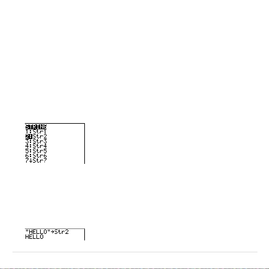
TI-83 Plus CATALOG, Strings, Hyperbolic Functions 487
Storing a String to a String Variable
To store a string to a string variable, follow these steps.
1. Press
ƒ
[
ã
], enter the string, and press
ƒ
[
ã
].
2. Press
¿
.
3. Press
7
to display the
VARS STRING
menu.
4. Select the string variable (from
Str1
to
Str9
, or
Str0
) to which you want
to store the string.
The string variable is pasted to the current cursor location, next to the
store symbol (
!
).
5. Press
Í
to store the string to the string variable. On the home
screen, the stored string is displayed on the next line without
quotation marks.
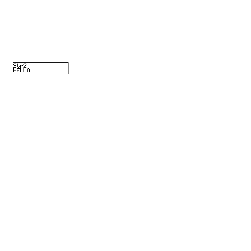
TI-83 Plus CATALOG, Strings, Hyperbolic Functions 488
Displaying the Contents of a String Variable
To display the contents of a string variable on the home screen, select
the string variable from the
VARS STRING
menu, and then press
Í
.
The string is displayed.

TI-83 Plus CATALOG, Strings, Hyperbolic Functions 489
String Functions and Instructions in the
CATALOG
Displaying String Functions and Instructions in the CATALOG
String functions and instructions are available only from the
CATALOG
.
The table below lists the string functions and instructions in the order in
which they appear among the other
CATALOG
menu items. The ellipses in
the table indicate the presence of additional
CATALOG
items.
CATALOG
...
Equ
4
String(
Converts an equation to a string.
expr(
Converts a string to an expression.
...
inString(
Returns a character’s place number.
...
length(
Returns a string’s character length.
...
String
4
Equ(
Converts a string to an equation.
sub(
Returns a string subset as a string.
...
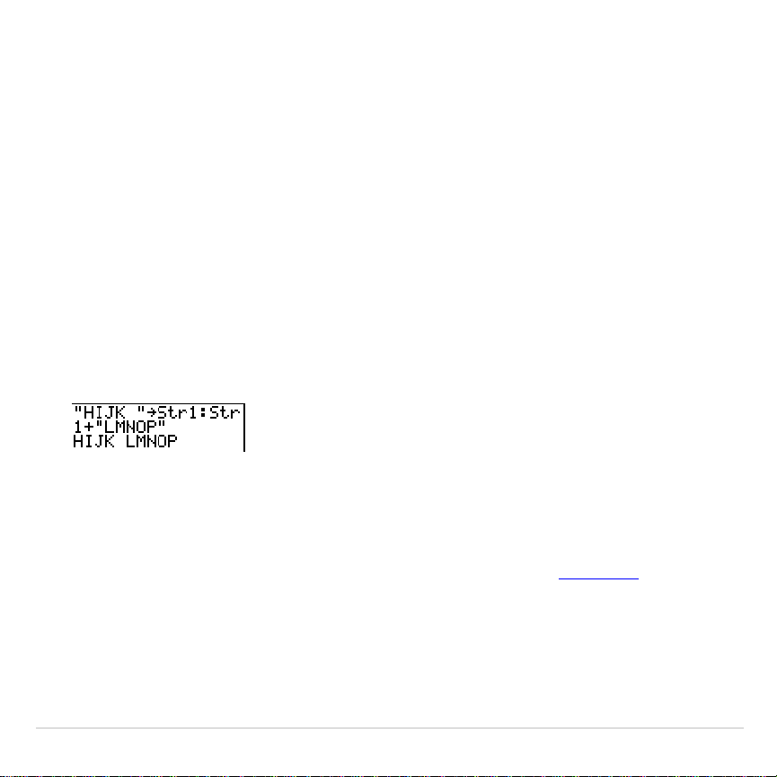
TI-83 Plus CATALOG, Strings, Hyperbolic Functions 490
+ (Concatenation)
To concatenate two or more strings, follow these steps.
1. Enter
string1
, which can be a string or string name.
2. Press
Ã
.
3. Enter
string2
, which can be a string or string name. If necessary,
press
Ã
and enter
string3
, and so on.
string1
+
string2
+
string3
. . .
4. Press
Í
to display the strings as a single string.
Selecting a String Function from the CATALOG
To select a string function or instruction and paste it to the current
screen, follow the steps for selecting an item from the
CATALOG
.
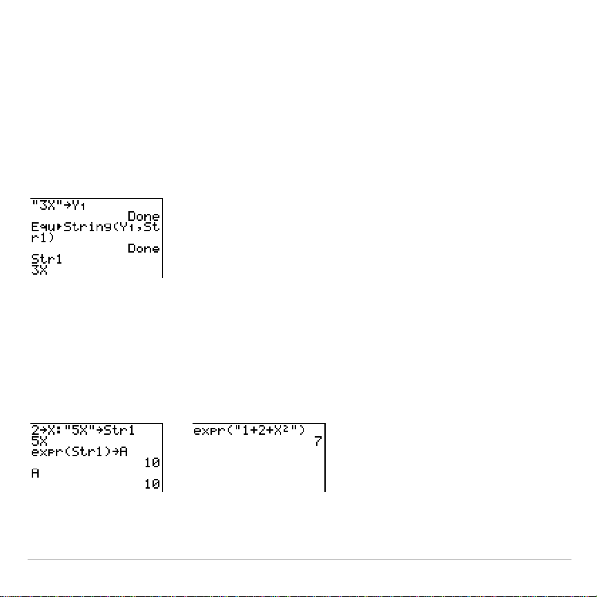
TI-83 Plus CATALOG, Strings, Hyperbolic Functions 491
Equ
4
String(
Equ
4
String(
converts to a string an equation that is stored to any
VARS
Y
.
VARS
variable.
Y
n
contains the equation.
Str
n
(from
Str1
to
Str9
, or
Str0
)
is the string variable to which you want the equation to be stored as a
string.
Equ
4
String(Y
n
,Str
n
)
expr(
expr(
converts the character string contained in
string
to an expression
and executes it.
string
can be a string or a string variable.
expr(
string
)
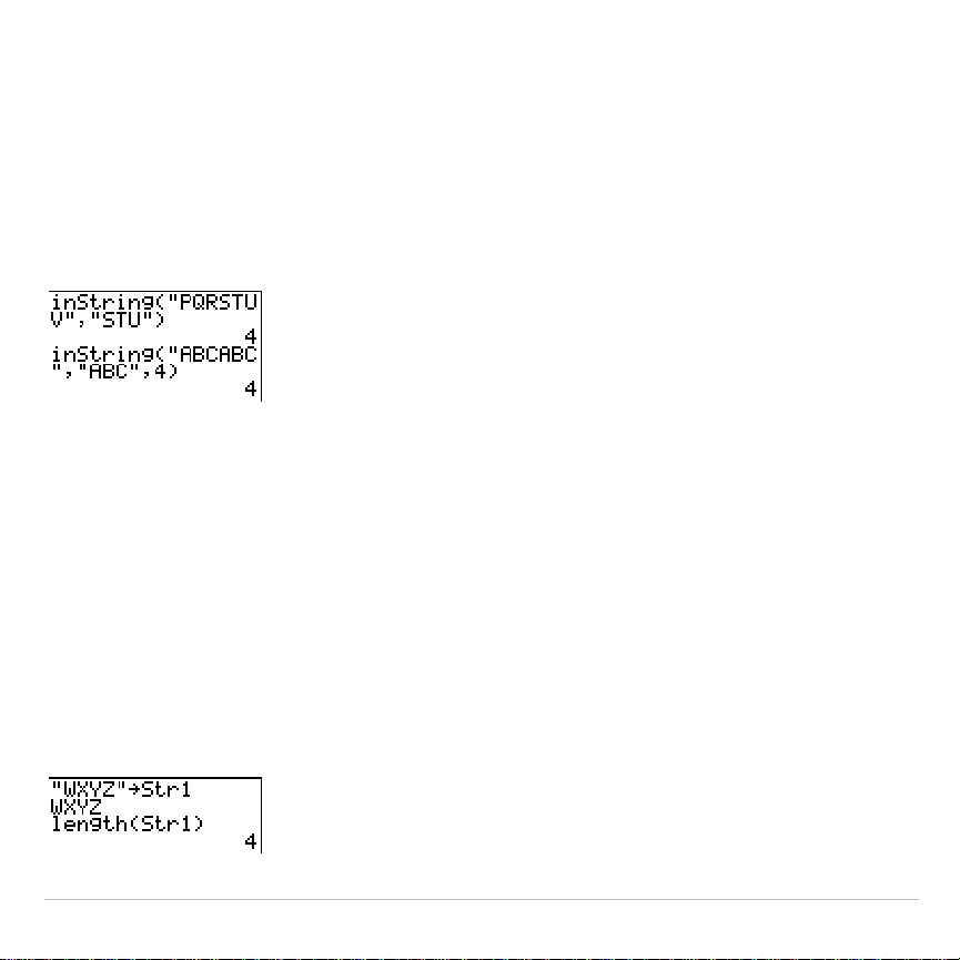
TI-83 Plus CATALOG, Strings, Hyperbolic Functions 492
inString(
inString(
returns the character position in
string
of the first character of
substring
.
string
can be a string or a string variable.
start
is an optional
character position at which to start the search; the default is 1.
inString(
string
,
substring
[
,
start
]
)
Note: If
string
does not contain
substring
, or
start
is greater than the length of
string
,
inString(
returns
0
.
length(
length(
returns the number of characters in
string
.
string
can be a string or
string variable.
Note: An instruction or function name, such as
sin(
or
cos(
, counts as one
character.
length(
string
)
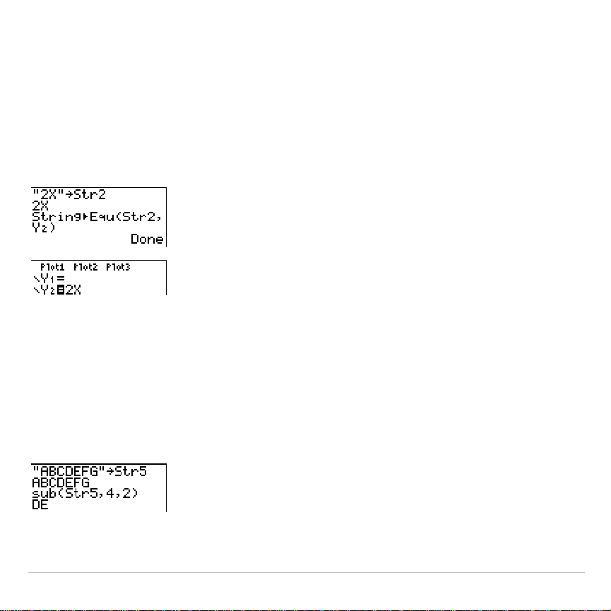
TI-83 Plus CATALOG, Strings, Hyperbolic Functions 493
String
4
Equ(
String
4
Equ(
converts
string
into an equation and stores the equation to
Y
n
.
string
can be a string or string variable.
String
4
Equ(
is the inverse of
Equ
4
String(
.
String
4
Equ(
string
,Y
n
)
sub(
sub(
returns a string that is a subset of an existing
string
.
string
can be a
string or a string variable.
begin
is the position number of the first
character of the subset.
length
is the number of characters in the subset.
sub(
string
,
begin
,
length
)
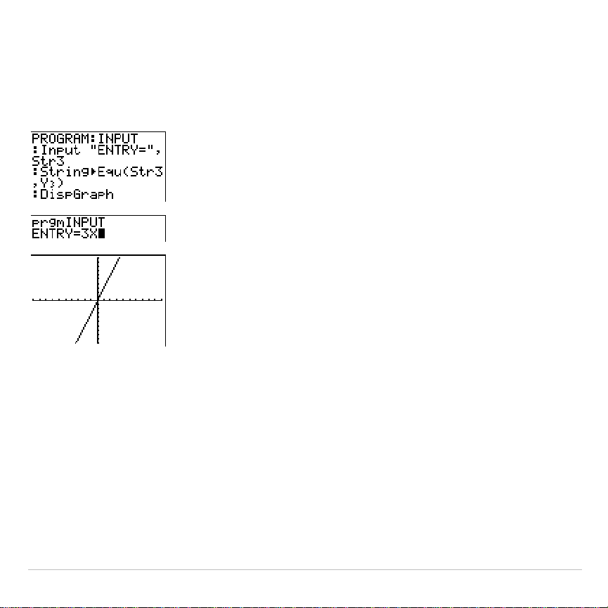
TI-83 Plus CATALOG, Strings, Hyperbolic Functions 494
Entering a Function to Graph during Program Execution
In a program, you can enter a function to graph during program
execution using these commands.
Note: When you execute this program, enter a function to store to
Y3
at the
ENTRY=
prompt.

TI-83 Plus CATALOG, Strings, Hyperbolic Functions 495
Hyperbolic Functions in the CATALOG
Hyperbolic Functions
The hyperbolic functions are available only from the
CATALOG
. The table
below lists the hyperbolic functions in the order in which they appear
among the other
CATALOG
menu items. The ellipses in the table indicate
the presence of additional
CATALOG
items.
CATALOG
...
cosh(
Hyperbolic cosine
cosh
L
1
(
Hyperbolic arccosine
...
sinh(
Hyperbolic sine
sinh
L
1
(
Hyperbolic arcsine
...
tanh(
Hyperbolic tangent
tanh
L
1
(
Hyperbolic arctangent
...
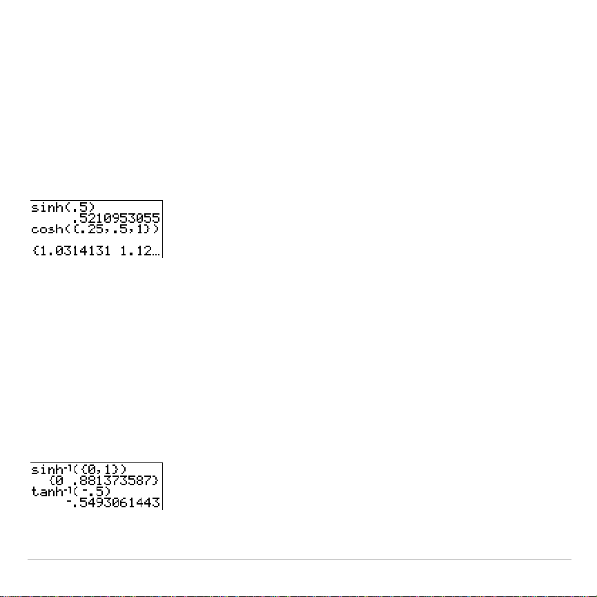
TI-83 Plus CATALOG, Strings, Hyperbolic Functions 496
sinh(, cosh(, tanh(
sinh(
,
cosh(
, and
tanh(
are the hyperbolic functions. Each is valid for real
numbers, expressions, and lists.
sinh(
value
)
cosh(
value
)
tanh(
value
)
sinh
L
1
(, cosh
L
1
(, tanh
L
1
(
sinh
L
1
(
is the hyperbolic arcsine function.
cosh
L
1
(
is the hyperbolic
arccosine function.
tanh
L
1
(
is the hyperbolic arctangent function. Each is
valid for real numbers, expressions, and lists.
sinh
L
1
(
value
)
cosh
L
1
(
value
)
sinh
L
1
(
value
)
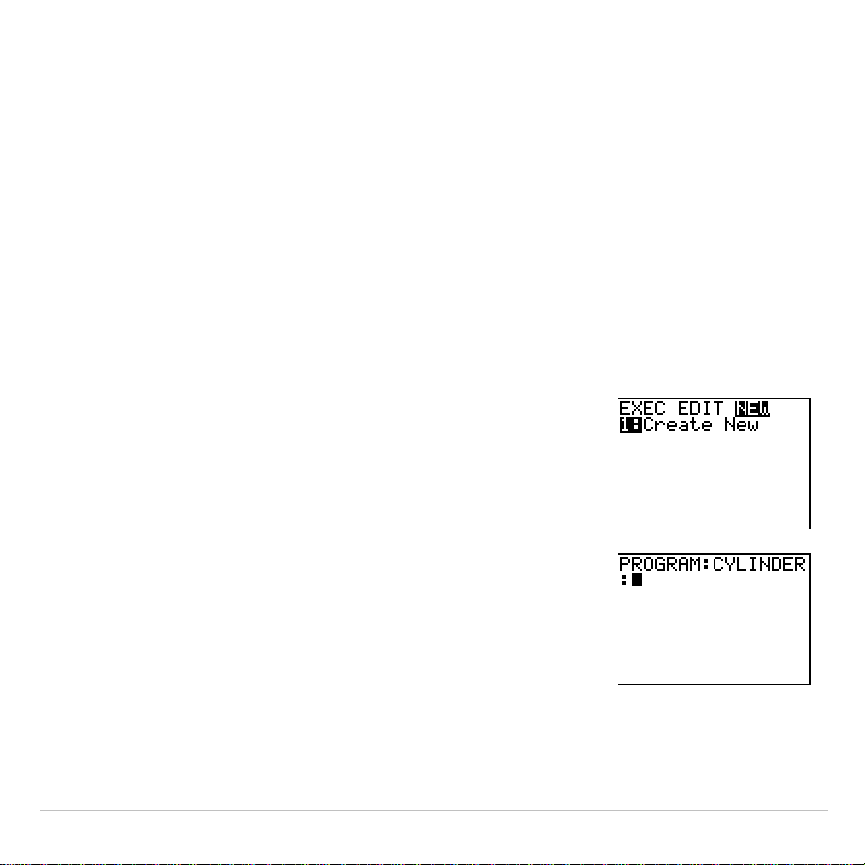
TI-83 Plus Programming 497
Chapter 16:
Programming
Getting Started: Volume of a Cylinder
Getting Started is a fast-paced introduction. Read the chapter for details.
A program is a set of commands that the TI-83 Plus executes sequentially, as if
you had entered them from the keyboard. Create a program that prompts for the
radius R and the height H of a cylinder and then computes its volume.
1. Press
~
~
to display the
PRGM NEW
menu.
2. Press
Í
to select
1:Create New
. The
Name=
prompt is displayed, and alpha-lock is on. Press
[
C
] [
Y
] [
L
] [
I
] [
N
] [
D
] [
E
] [
R
], and then press
Í
to
name the program
CYLINDER
.
You are now in the program editor. The colon
(
:
) in the first column of the second line
indicates the beginning of a command line.
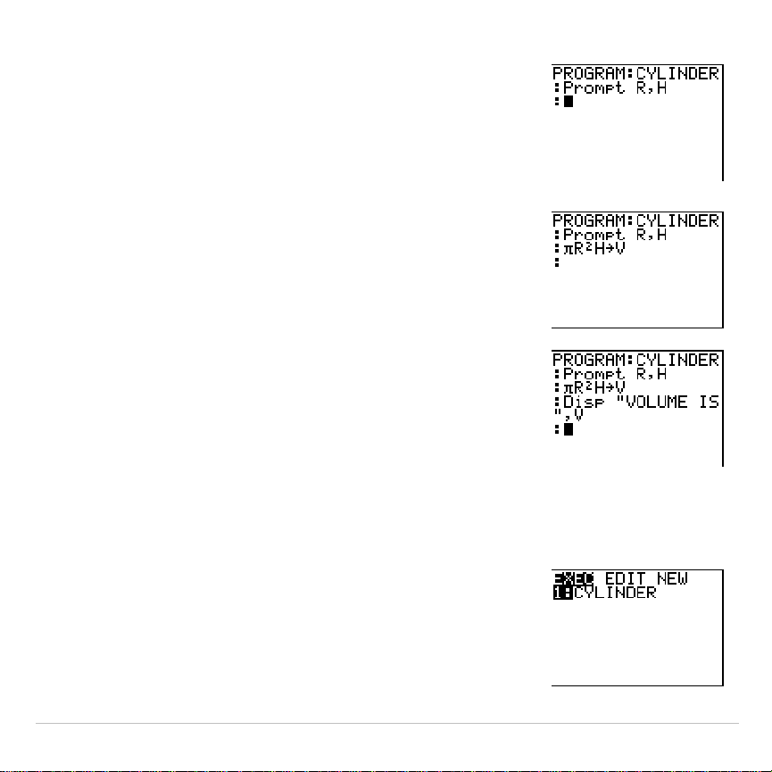
TI-83 Plus Programming 498
3. Press
~
2
to select
2:Prompt
from the
PRGM I/O
menu.
Prompt
is copied to the
command line. Press
ƒ
[
R
]
¢
ƒ
[
H
] to
enter the variable names for radius and height.
Press
Í
.
4. Press
y
ãpä
ƒ
[
R
]
¡
ƒ
[
H
]
¿
ƒ
[
V
]
Í
to enter the expression
p
R
2
H
and store it to the variable
V
.
5. Press
~
3
to select
3:Disp
from the
PRGM
I/O
menu.
Disp
is pasted to the command line.
Press
y
7
ã
ã
ä
[
V
] [
O
] [
L
] [
U
] [
M
] [
E
][
'
] [
I
] [
S
]
ã
ã
ä
ƒ
¢
ƒ
[
V
]
Í
to set up the
program to display the text
VOLUME IS
on one
line and the calculated value of
V
on the next.
6. Press
y
5
to display the home screen.
7. Press
to display the
PRGM EXEC
menu. The
items on this menu are the names of stored
programs.
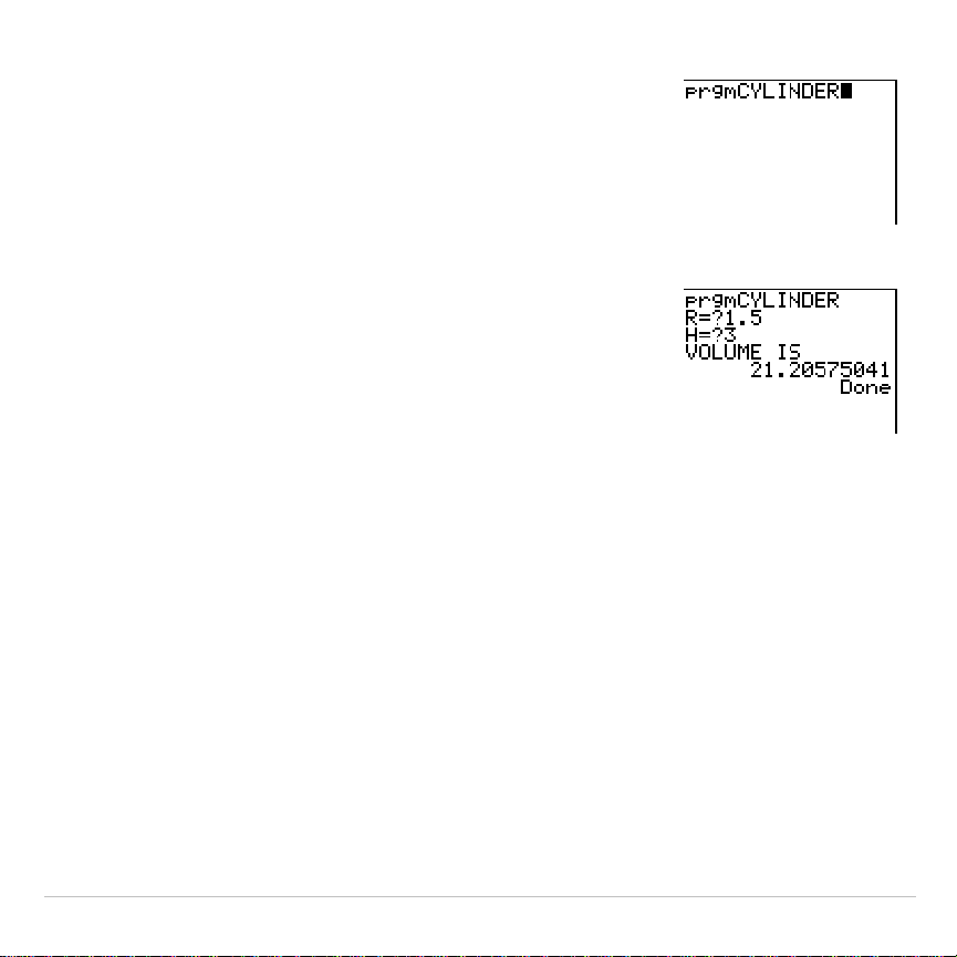
TI-83 Plus Programming 499
8. Press
Í
to paste
prgmCYLINDER
to the
current cursor location. (If
CYLINDER
is not item
1
on your
PRGM EXEC
menu, move the cursor to
CYLINDER
before you press
Í
.)
9. Press
Í
to execute the program. Enter
1.5
for the radius, and then press
Í
. Enter
3
for
the height, and then press
Í
. The text
VOLUME IS
, the value of
V
, and
Done
are
displayed.
Repeat steps 7 through 9 and enter different
values for
R
and
H
.
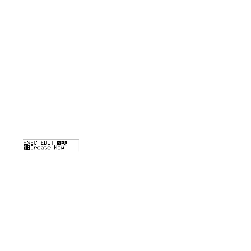
TI-83 Plus Programming 500
Creating and Deleting Programs
What Is a Program?
A program is a set of one or more command lines. Each line contains
one or more instructions. When you execute a program, the TI-83 Plus
performs each instruction on each command line in the same order in
which you entered them. The number and size of programs that the
TI-83 Plus can store is limited only by available memory.
Creating a New Program
To create a new program, follow these steps.
1. Press
|
to display the
PRGM NEW
menu.
2. Press
Í
to select
1:Create New
. The
Name=
prompt is displayed,
and alpha-lock is on.
3. Press a letter from A to Z or
q
to enter the first character of the new
program name.
Note: A program name can be one to eight characters long. The first
character must be a letter from A to Z or
q
. The second through eighth
characters can be letters, numbers, or
q
.
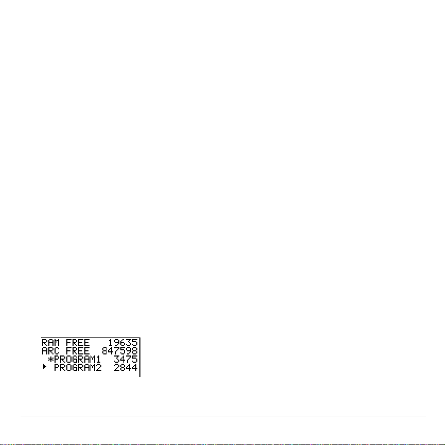
TI-83 Plus Programming 501
4. Enter zero to seven letters, numbers, or
q
to complete the new
program name.
5. Press
Í
. The program editor is displayed.
6. Enter one or more program commands.
7. Press
y
5
to leave the program editor and return to the home
screen.
Managing Memory and Deleting a Program
To check whether adequate memory is available for a program you want
to enter:
1. Press
y
L
to display the
MEMORY
menu.
2.Select
2:Mem Mgmt/Del
to display the
MEMORY MANAGEMENT/DELETE
menu (Chapter 18).
3. Select
7:Prgm
to display the PRGM editor.
The TI-83 Plus expresses memory quantities in bytes.

TI-83 Plus Programming 502
You can increase available memory in one of two ways. You can delete
one or more programs or you can archive some programs.
To increase available memory by deleting a specific program:
1. Press
y
L
and then select
2:Mem Mgmt/Del
from the
MEMORY
menu.
2. Select
7:Prgm
to display the PRGM editor (Chapter 18).
3. Press
}
and
†
to move the selection cursor (
4
) next to the program
you want to delete, and then press
{
. The program is deleted from
memory.
Note: You will receive a message asking you to confirm this delete action.
Select
2:yes
to continue.
To leave the PRGM editor screen without deleting anything, press
y
5
, which displays the home screen.
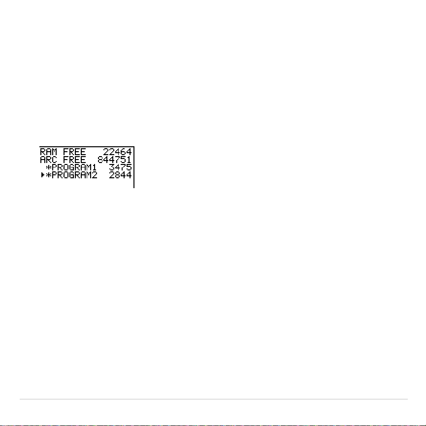
TI-83 Plus Programming 503
To increase available memory by archiving a program:
1. Press
y
L
and then select
2:Mem Mgmt/Del
from the
MEMORY
menu.
2. Select
2:Mem Mgmt/Del
to display the
MEM MGMT/DEL
menu.
3. Select
7:Prgm...
to display the
PRGM
menu.
4. Press
Í
to archive the program. An asterisk will appear to the left
of the program to indicate it is an archived program.
To unarchive a program in this screen, put the cursor next to the
archived program and press
Í
. The asterisk will disappear.
Note: Archive programs cannot be edited or executed. In order to edit or
execute an archived program, you must first unarchive it.

TI-83 Plus Programming 504
Entering Command Lines and Executing
Programs
Entering a Program Command Line
You can enter on a command line any instruction or expression that you
could execute from the home screen. In the program editor, each new
command line begins with a colon. To enter more than one instruction or
expression on a single command line, separate each with a colon.
Note: A command line can be longer than the screen is wide; long command
lines wrap to the next screen line.
While in the program editor, you can display and select from menus. You
can return to the program editor from a menu in either of two ways.
•
Select a menu item, which pastes the item to the current command line.
•
Press
‘
.
When you complete a command line, press
Í
. The cursor moves to
the next command line.
Programs can access variables, lists, matrices, and strings saved in
memory. If a program stores a new value to a variable, list, matrix, or
string, the program changes the value in memory during execution.
You can call another program as a subroutine.

TI-83 Plus Programming 505
Executing a Program
To execute a program, begin on a blank line on the home screen and
follow these steps.
1. Press
to display the
PRGM EXEC
menu.
2. Select a program name from the
PRGM EXEC
menu.
prgm
name
is
pasted to the home screen (for example,
prgmCYLINDER
).
3. Press
Í
to execute the program. While the program is executing,
the busy indicator is on.
Last Answer (
Ans
) is updated during program execution. Last Entry is
not updated as each command is executed (Chapter 1).
The TI-83 Plus checks for errors during program execution. It does not
check for errors as you enter a program.

TI-83 Plus Programming 506
Breaking a Program
To stop program execution, press
É
. The
ERR:BREAK
menu is displayed.
•
To return to the home screen, select
1:Quit
.
•
To go where the interruption occurred, select
2:Goto
.

TI-83 Plus Programming 507
Editing Programs
Editing a Program
To edit a stored program, follow these steps.
1. Press
~
to display the
PRGM EDIT
menu.
2. Select a program name from the
PRGM EDIT
menu. Up to the first
seven lines of the program are displayed.
Note: The program editor does not display a
$
to indicate that a program
continues beyond the screen.
3. Edit the program command lines.
•
Move the cursor to the appropriate location, and then delete,
overwrite, or insert.
•
Press
‘
to clear all program commands on the command line
(the leading colon remains), and then enter a new program
command.
Tip: To move the cursor to the beginning of a command line, press
y
|
; to
move to the end, press
y
~
. To scroll the cursor down seven command lines,
press
ƒ
†
. To scroll the cursor up seven command lines, press
ƒ
}
.

TI-83 Plus Programming 508
Inserting and Deleting Command Lines
To insert a new command line anywhere in the program, place the
cursor where you want the new line, press
y
6
, and then press
Í
. A colon indicates a new line.
To delete a command line, place the cursor on the line, press
‘
to
clear all instructions and expressions on the line, and then press
{
to
delete the command line, including the colon.

TI-83 Plus Programming 509
Copying and Renaming Programs
Copying and Renaming a Program
To copy all command lines from one program into a new program, follow
steps 1 through 5 for
Creating a New Program
, and then follow these
steps.
1. Press
y
K
.
Rcl
is displayed on the bottom line of the program
editor in the new program (Chapter 1).
2. Press
|
to display the
PRGM EXEC
menu.
3. Select a name from the menu.
prgm
name
is pasted to the bottom line
of the program editor.
4. Press
Í
. All command lines from the selected program are
copied into the new program.
Copying programs has at least two convenient applications.
•
You can create a template for groups of instructions that you use
frequently.
•
You can rename a program by copying its contents into a new
program.

TI-83 Plus Programming 510
Note:
You also can copy all the command lines from one existing program to
another existing program using
RCL
.
Scrolling the PRGM EXEC and PRGM EDIT Menus
The TI-83 Plus sorts
PRGM EXEC
and
PRGM EDIT
menu items automatically
into alphanumerical order. Each menu only labels the first 10 items using
1
through
9
, then
0
.
To jump to the first program name that begins with a particular alpha
character or
q
, press
ƒ
[
letter from A to Z or
q
].
Tip:
From the top of either the
PRGM EXEC
or
PRGM EDIT
menu, press
}
to
move to the bottom. From the bottom, press
†
to move to the top. To scroll the
cursor down the menu seven items, press
ƒ
†
. To scroll the cursor up the
menu seven items, press
ƒ
}
.
TI-83 Plus Programming 511
PRGM CTL (Control) Instructions
PRGM CTL Menu
To display the
PRGM CTL
(program control) menu, press
from the
program editor only.
CTL I/O EXEC
1:If
Creates a conditional test.
2:Then
Executes commands when
If
is true.
3:Else
Executes commands when
If
is false.
4:For(
Creates an incrementing loop.
5:While
Creates a conditional loop.
6:Repeat
Creates a conditional loop.
7:End
Signifies the end of a block.
8:Pause
Pauses program execution.
9:Lbl
Defines a label.
0:Goto
Goes to a label.
A:IS>(
Increments and skips if greater than.
B:DS<(
Decrements and skips if less than.
C:Menu(
Defines menu items and branches.
D:prgm
Executes a program as a subroutine.
E:Return
Returns from a subroutine.
F:Stop
Stops execution.
G:DelVar
Deletes a variable from within program.
H:GraphStyle(
Designates the graph style to be drawn.

TI-83 Plus Programming 512
These menu items direct the flow of an executing program. They make it
easy to repeat or skip a group of commands during program execution.
When you select an item from the menu, the name is pasted to the
cursor location on a command line in the program.
To return to the program editor without selecting an item, press
‘
.
Controlling Program Flow
Program control instructions tell the TI-83 Plus which command to
execute next in a program.
If
,
While
, and
Repeat
check a defined
condition to determine which command to execute next. Conditions
frequently use relational or Boolean tests (Chapter 2), as in:
If A<7:A+1
!
A
or
If N=1 and M=1:Goto Z
If
Use
If
for testing and branching. If
condition
is false (zero), then the
command
immediately following
If
is skipped. If
condition
is true (nonzero),
then the next
command
is executed.
If
instructions can be nested.
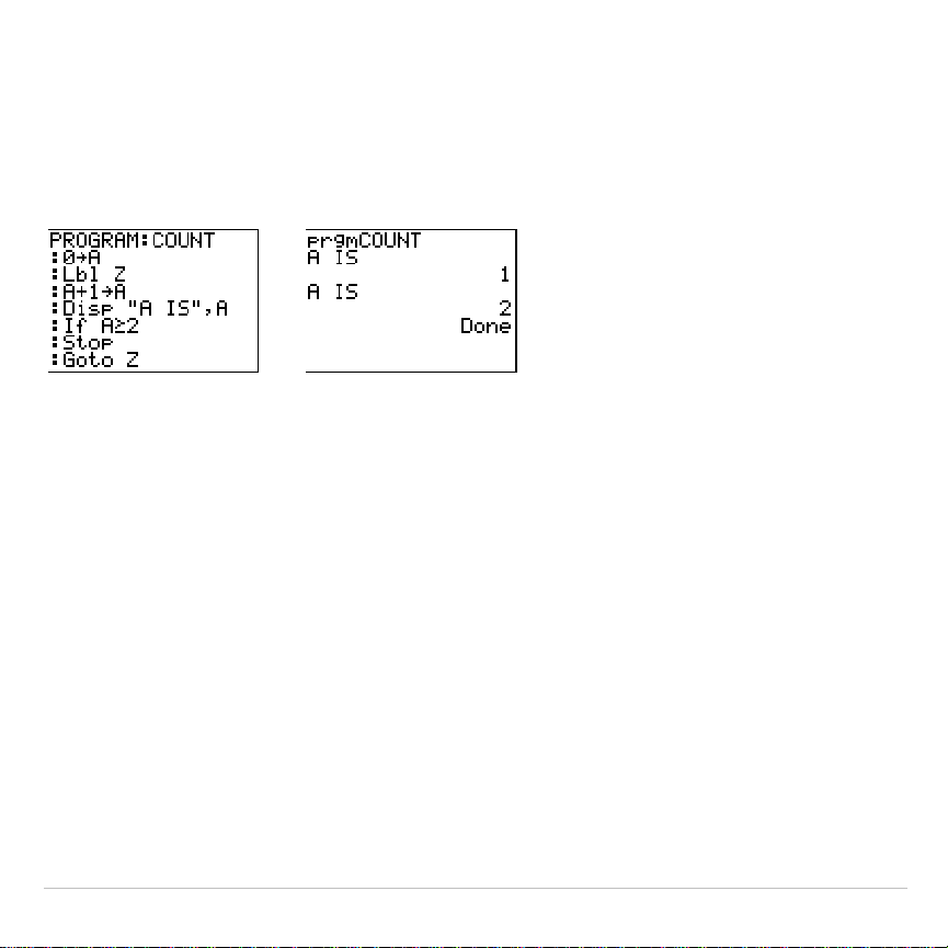
TI-83 Plus Programming 513
:If
condition
:
command
(if true)
:
command
Program Output
If
.
Then
Then
following an
If
executes a group of
commands
if
condition
is true
(nonzero).
End
identifies the end of the group of
commands
.
:If
condition
:Then
:
command
(if true)
:
command
(if true)
:End
:
command
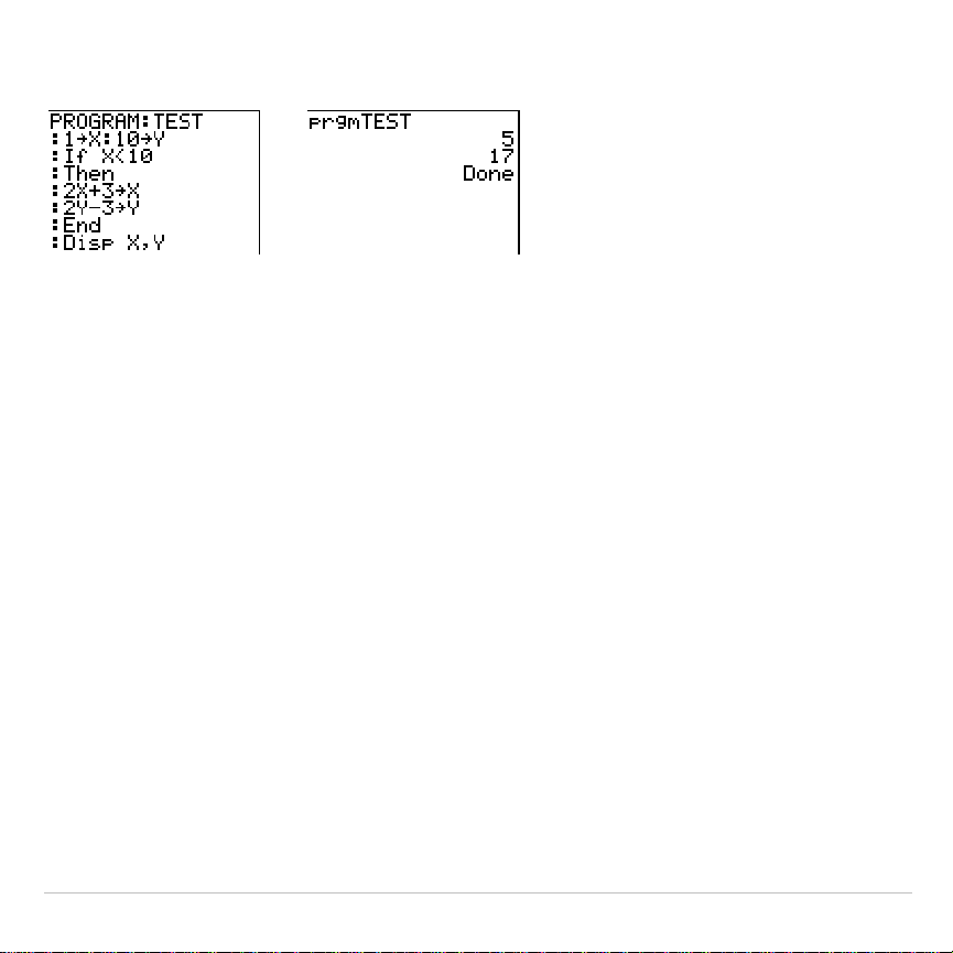
TI-83 Plus Programming 514
Program Output
If
.
Then
.
Else
Else
following
If
.
Then
executes a group of
commands
if
condition
is false
(zero).
End
identifies the end of the group of
commands
.
:If
condition
:Then
:
command
(if true)
:
command
(if true)
:Else
:
command
(if false)
:
command
(if false)
:End
:
command
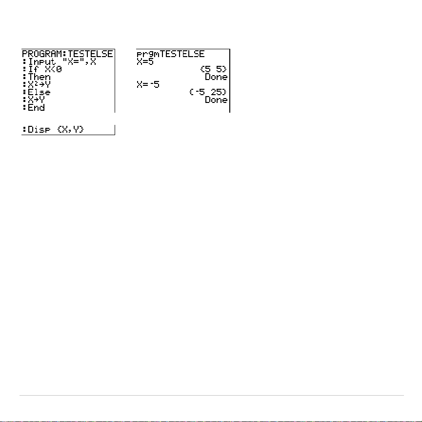
TI-83 Plus Programming 515
Program Output
For(
For(
loops and increments. It increments
variable
from
begin
to
end
by
increment
.
increment
is optional (default is 1) and can be negative
(
end
<
begin
).
end
is a maximum or minimum value not to be exceeded.
End
identifies the end of the loop.
For(
loops can be nested.
:For(
variable
,
begin
,
end
[
,
increment
]
)
:
command
(while
end
not exceeded)
:
command
(while
end
not exceeded)
:End
:
command
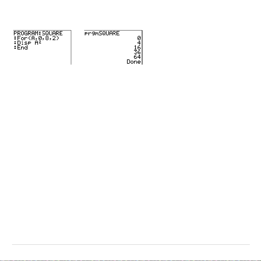
TI-83 Plus Programming 516
Program Output
While
While
performs a group of
commands
while
condition
is true.
condition
is
frequently a relational test (Chapter 2).
condition
is tested when
While
is
encountered. If
condition
is true (nonzero), the program executes a group
of
commands
.
End
signifies the end of the group. When
condition
is false
(zero), the program executes each
command
following
End
.
While
instructions can be nested.
:While
condition
:
command
(while
condition
is true)
:
command
(while
condition
is true)
:End
:
command
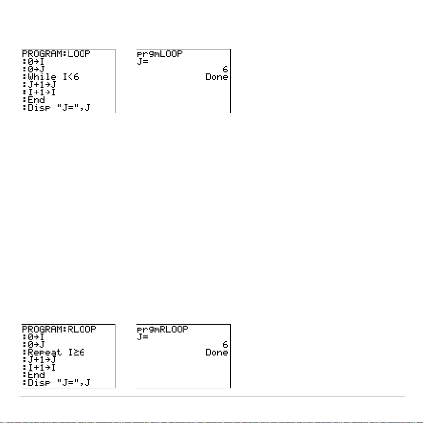
TI-83 Plus Programming 517
Program Output
Repeat
Repeat
repeats a group of
commands
until
condition
is true (nonzero). It is
similar to
While
, but
condition
is tested when
End
is encountered;
therefore, the group of
commands
is always executed at least once.
Repeat
instructions can be nested.
:Repeat
condition
:
command
(until
condition
is true)
:
command
(until
condition
is true)
:End
:
c
ommand
Program Output

TI-83 Plus Programming 518
End
End
identifies the end of a group of
commands
. You must include an
End
instruction at the end of each
For(
,
While
, or
Repeat
loop. Also, you must
paste an
End
instruction at the end of each
If
.
Then
group and each
If
.
Then
.
Else
group.
Pause
Pause
suspends execution of the program so that you can see answers
or graphs. During the pause, the pause indicator is on in the top-right
corner. Press
Í
to resume execution.
•
Pause
without a
value
temporarily pauses the program. If the
DispGraph
or
Disp
instruction has been executed, the appropriate
screen is displayed.
•
Pause
with
value
displays
value
on the current home screen.
value
can
be scrolled.
Pause
[
value
]
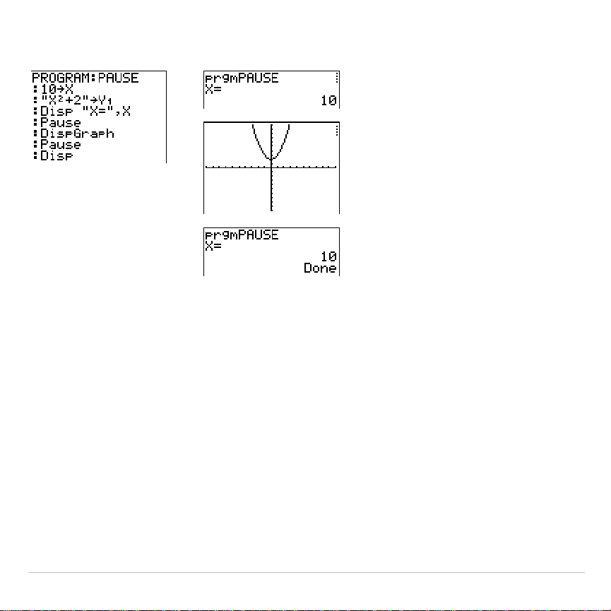
TI-83 Plus Programming 519
Program Output
Lbl, Goto
Lbl
(label) and
Goto
(go to) are used together for branching.
Lbl
specifies the
label
for a command.
label
can be one or two characters
(
A
through
Z
,
0
through
99
, or
q
).
Lbl
label
Goto
causes the program to branch to
label
when
Goto
is encountered.
Goto
label
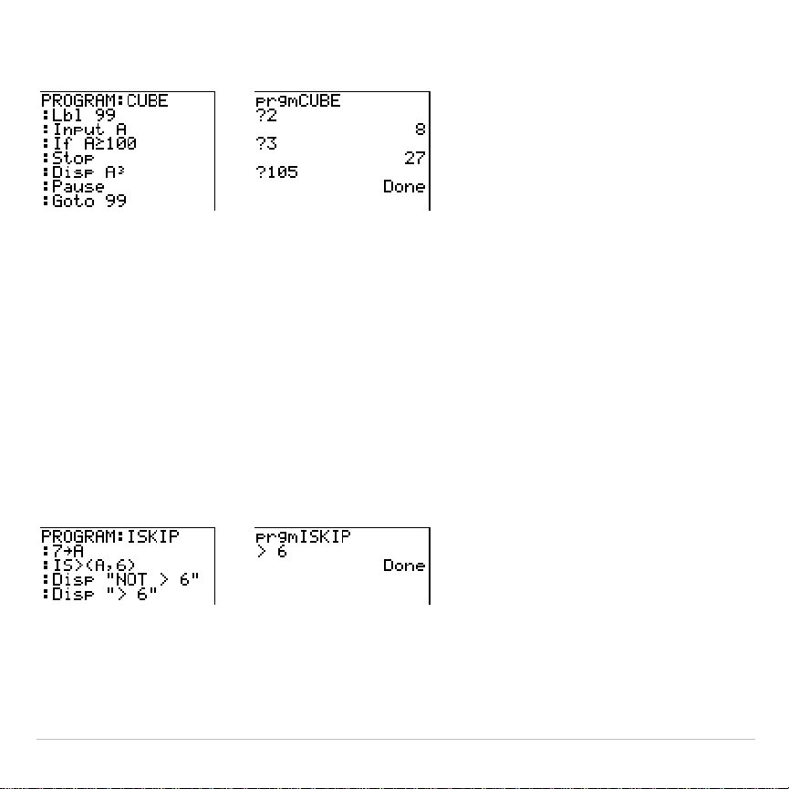
TI-83 Plus Programming 520
Program Output
IS>(
IS>(
(increment and skip) adds 1 to
variable.
If the answer is >
value
(which
can be an expression), the next
command
is skipped; if the answer is
{
value
, the next
command
is executed.
variable
cannot be a system variable.
:IS>(
variable
,
value
)
:
command
(if answer
value
)
:
command
(if answer >
value
)
Program Output
Note:
IS>(
is not a looping instruction.

TI-83 Plus Programming 521
DS<(
DS<(
(decrement and skip) subtracts 1 from
variable
. If the answer is
<
value
(which can be an expression), the next
command
is skipped; if the
answer is
|
value
, the next
command
is executed.
variable
cannot be a
system variable.
:DS<(
variable
,
value
)
:
command
(if answer
‚
value
)
:
command
(if answer <
value
)
Program Output
Note:
DS<(
is not a looping instruction.
Menu(
Menu(
sets up branching within a program. If
Menu(
is encountered during
program execution, the menu screen is displayed with the specified
menu items, the pause indicator is on, and execution pauses until you
select a menu item.
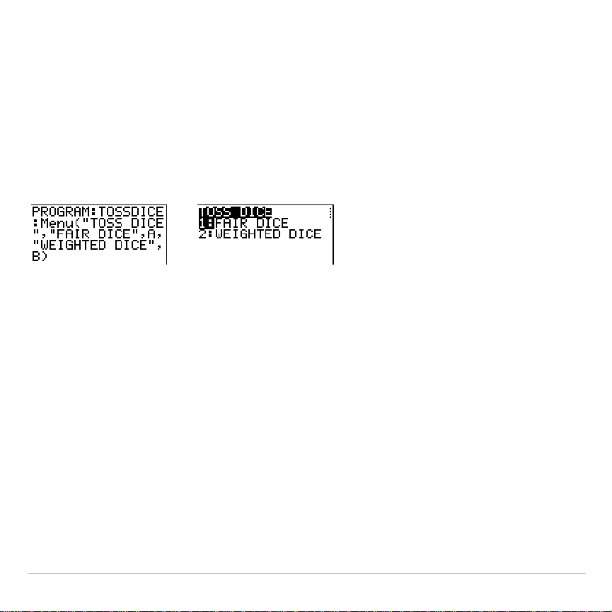
TI-83 Plus Programming 522
The menu
title
is enclosed in quotation marks (
"
). Up to seven pairs of
menu items follow. Each pair comprises a
text
item (also enclosed in
quotation marks) to be displayed as a menu selection, and a
label
item to
which to branch if you select the corresponding menu selection.
Menu("
title
","
text1
",
label1
,"
text2
",
label2
,
. . .
)
Program Output
The program above pauses until you select
1
or
2
. If you select
2
, for
example, the menu disappears and the program continues execution at
Lbl B
.
prgm
Use
prgm
to execute other programs as subroutines. When you select
prgm
, it is pasted to the cursor location. Enter characters to spell a
program
name
. Using
prgm
is equivalent to selecting existing programs
from the
PRGM EXEC
menu; however, it allows you to enter the name of a
program that you have not yet created.
prgm
name
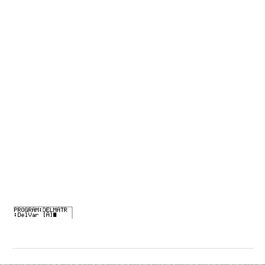
TI-83 Plus Programming 523
Note:
You cannot directly enter the subroutine name when using
RCL
. You
must paste the name from the
PRGM EXEC
menu.
Return
Return
quits the subroutine and returns execution to the calling program,
even if encountered within nested loops. Any loops are ended. An
implied
Return
exists at the end of any program that is called as a
subroutine. Within the main program,
Return
stops execution and returns
to the home screen.
Stop
Stop
stops execution of a program and returns to the home screen.
Stop
is optional at the end of a program.
DelVar
DelVar
deletes from memory the contents of
variable
.
DelVar
variable

TI-83 Plus Programming 524
GraphStyle(
GraphStyle(
designates the style of the graph to be drawn.
function#
is the
number of the
Y=
function name in the current graphing mode.
graphstyle
is a number from
1
to
7
that corresponds to the graph style, as shown
below.
1
=
ç
(line)
5
=
ë
(path)
2
=
è
(thick)
6
=
ì
(animate)
3
=
é
(shade above)
7
=
í
(dot)
4
=
ê
(shade below)
GraphStyle(
function#
,
graphstyle
)
For example,
GraphStyle(1,5)
in
Func
mode sets the graph style for
Y1
to
ë
(path;
5
).
Not all graph styles are available in all graphing modes. For a detailed
description of each graph style, see the Graph Styles table in Chapter 3.

TI-83 Plus Programming 525
PRGM I/O (Input/Output) Instructions
PRGM I/O Menu
To display the
PRGM I/O
(program input/output) menu, press
~
from
within the program editor only.
CTL I/O EXEC
1:Input
Enters a value or uses the cursor.
2:Prompt
Prompts for entry of variable values.
3:Disp
Displays text, value, or the home screen.
4:DispGraph
Displays the current graph.
5:DispTable
Displays the current table.
6:Output(
Displays text at a specified position.
7:getKey
Checks the keyboard for a keystroke.
8:ClrHome
Clears the display.
9:ClrTable
Clears the current table.
0:GetCalc(
Gets a variable from another TI-83 Plus.
A:Get(
Gets a variable from CBL 2™/CBL™ or CBR™.
B:Send(
Sends a variable to CBL 2/CBL or CBR.
These instructions control input to and output from a program during
execution. They allow you to enter values and display answers during
program execution.
To return to the program editor without selecting an item, press
‘
.
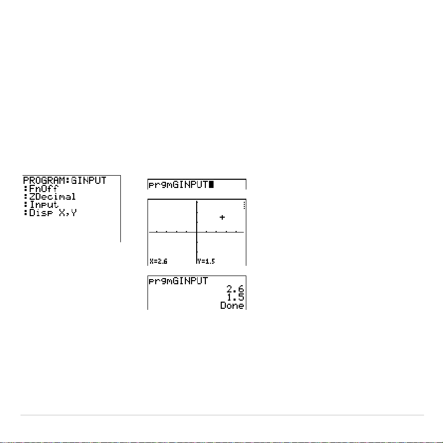
TI-83 Plus Programming 526
Displaying a Graph with Input
Input
without a variable displays the current graph. You can move the
free-moving cursor, which updates
X
and
Y
(and
R
and
q
for
PolarGC
format). The pause indicator is on. Press
Í
to resume program
execution.
Input
Program Output
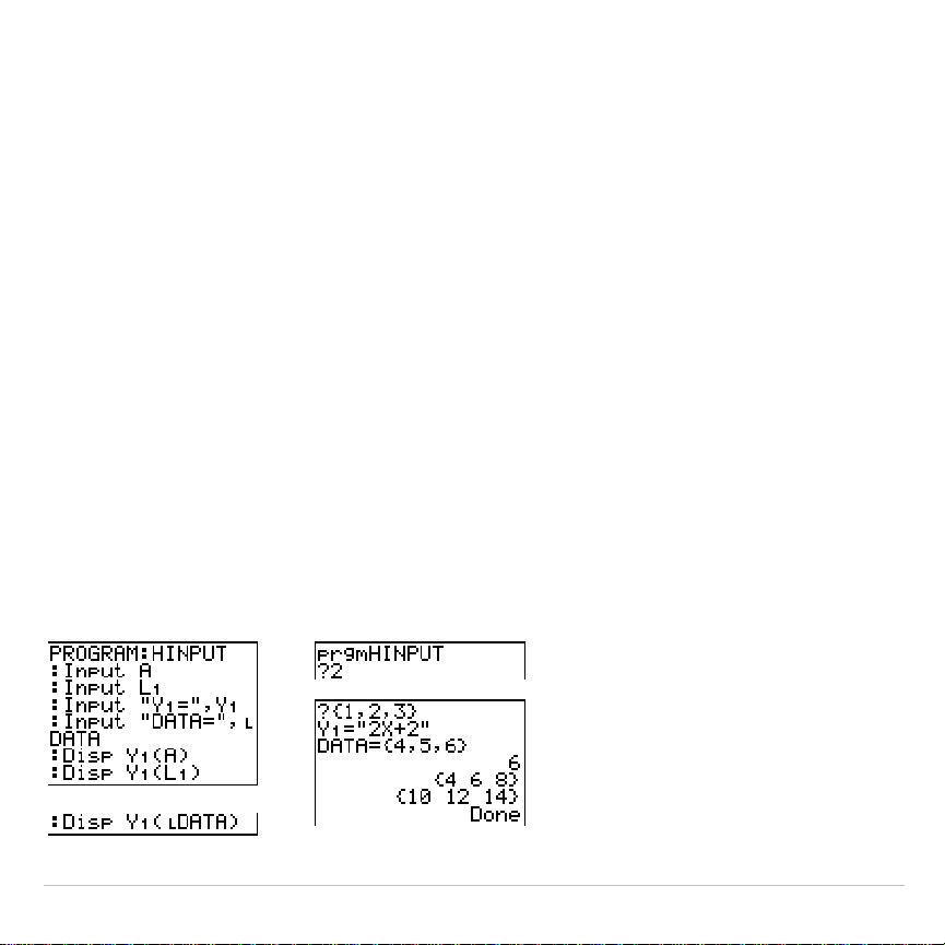
TI-83 Plus Programming 527
Storing a Variable Value with Input
Input
with
variable
displays a
?
(question mark) prompt during execution.
variable
may be a real number, complex number, list, matrix, string, or
Y=
function. During program execution, enter a value, which can be an
expression, and then press
Í
. The value is evaluated and stored to
variable
, and the program resumes execution.
Input
[
variable
]
You can display
text
or the contents of
Str
n
(a string variable) of up to 16
characters as a prompt. During program execution, enter a value after
the prompt and then press
Í
. The value is stored to
variable
, and the
program resumes execution.
Input
[
"
text
",
variable
]
Input
[
Str
n
,
variable
]
Program Output
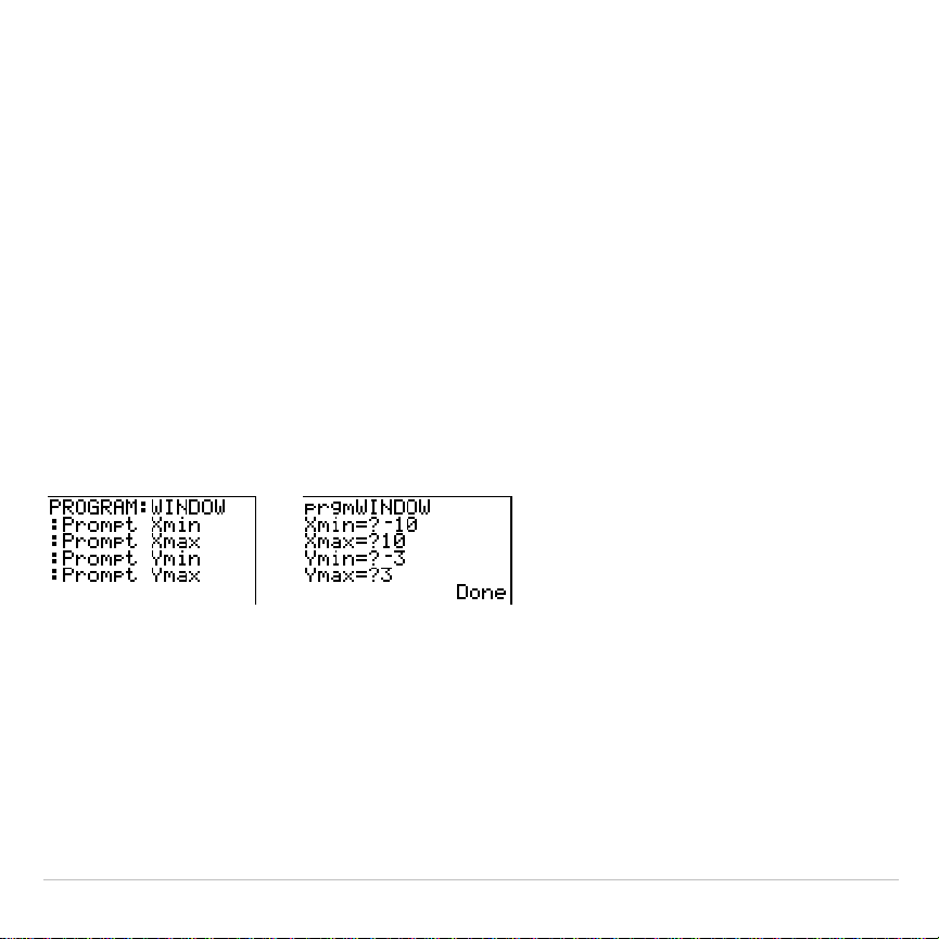
TI-83 Plus Programming 528
Note:
When a program prompts for input of lists and
Y
n
functions during
execution, you must include the braces (
{ }
) around the list elements and
quotation marks (
"
) around the expressions.
Prompt
During program execution,
Prompt
displays each
variable
, one at a time,
followed by
=?
. At each prompt, enter a value or expression for each
variable
, and then press
Í
. The values are stored, and the program
resumes execution.
Prompt
variableA
[
,
variableB
,
...
,
variable n
]
Program Output
Note:
Y= functions are not valid with
Prompt
.
Displaying the Home Screen
Disp
(display) without a value displays the home screen. To view the
home screen during program execution, follow the
Disp
instruction with a
Pause
instruction.
Disp
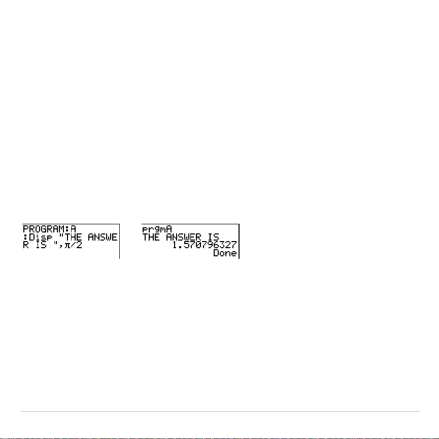
TI-83 Plus Programming 529
Displaying Values and Messages
Disp
with one or more
values
displays the value of each.
Disp
[
valueA
,
valueB
,
valueC
,
...
,
value n
]
•
If
value
is a variable, the current value is displayed.
•
If
value
is an expression, it is evaluated and the result is displayed on
the right side of the next line.
•
If
value
is text within quotation marks, it is displayed on the left side of
the current display line.
!
is not valid as text.
Program Output
If
Pause
is encountered after
Disp
, the program halts temporarily so you
can examine the screen. To resume execution, press
Í
.
Note: If a matrix or list is too large to display in its entirety, ellipses (...) are
displayed in the last column, but the matrix or list cannot be scrolled. To scroll,
use
Pause
value
.

TI-83 Plus Programming 530
DispGraph
DispGraph
(display graph) displays the current graph. If
Pause
is
encountered after
DispGraph
, the program halts temporarily so you can
examine the screen. Press
Í
to resume execution.
DispTable
DispTable
(display table) displays the current table. The program halts
temporarily so you can examine the screen. Press
Í
to resume
execution.
Output(
Output(
displays
text
or
value
on the current home screen beginning at
row
(
1
through
8
) and
column
(
1
through
16
), overwriting any existing
characters.
Tip: You may want to precede
Output(
with
ClrHome
.
Expressions are evaluated and values are displayed according to the
current mode settings. Matrices are displayed in entry format and wrap
to the next line.
!
is not valid as text.
Output(
row
,
column
,"
text
")
Output(
row
,
column
,
value
)
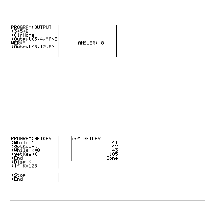
TI-83 Plus Programming 531
Program Output
For
Output(
on a
Horiz
split screen, the maximum value for
row
is 4.
getKey
getKey
returns a number corresponding to the last key pressed,
according to the key code diagram below. If no key has been pressed,
getKey
returns 0. Use
getKey
inside loops to transfer control, for
example, when creating video games.
Program Output
Note:
,
Œ
,
, and
Í
were pressed during
program execution.
Note:
You can press
É
at any time during execution to break the program.
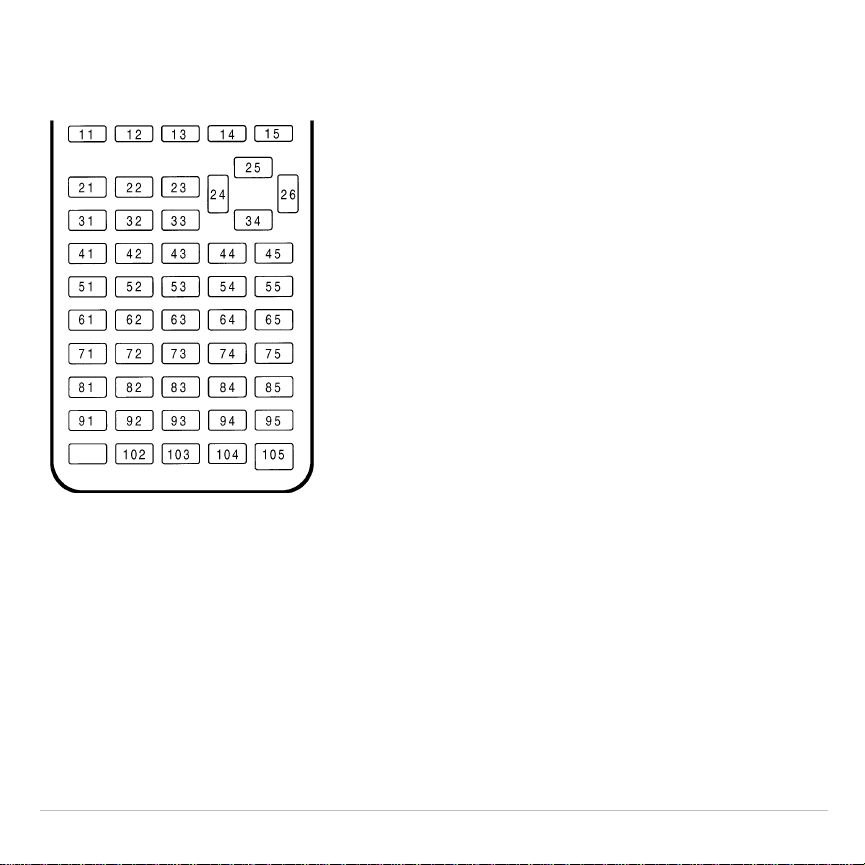
TI-83 Plus Programming 532
TI-83 Plus Key Code Diagram
ClrHome, ClrTable
ClrHome
(clear home screen) clears the home screen during program
execution.
ClrTable
(clear table) clears the values in the table during program
execution.

TI-83 Plus Programming 533
GetCalc(
GetCalc(
gets the contents of
variable
on another TI-83 Plus and stores it
to
variable
on the receiving TI-83 Plus.
variable
can be a real or complex
number, list element, list name, matrix element, matrix name, string,
Y=
variable, graph database, or picture.
GetCalc(
variable
)
Note:
GetCalc(
does not work between TI
.
82 and TI-83 Plus calculators.
Get(, Send(
Get(
gets data
from the CBL 2/CBL or CBR and stores it to
variable
on the
receiving TI-83 Plus.
variable
can be a real number, list element, list
name, matrix element, matrix name, string,
Y=
variable, graph database,
or picture.
Get(
variable
)
Note: If you transfer a program that references the
Get(
command to the
TI-83 Plus from a TI
.
82, the TI-83 Plus will interpret it as the
Get(
described
above. Use
GetCalc(
to get data from another TI-83 Plus.
Send(
sends the contents of
variable
to the CBL 2/CBL or CBR. You
cannot use it to send to another TI-83 Plus.
variable
can be a real
number, list element, list name, matrix element, matrix name, string,
Y=
variable, graph database, or picture.
variable
can be a list of elements.
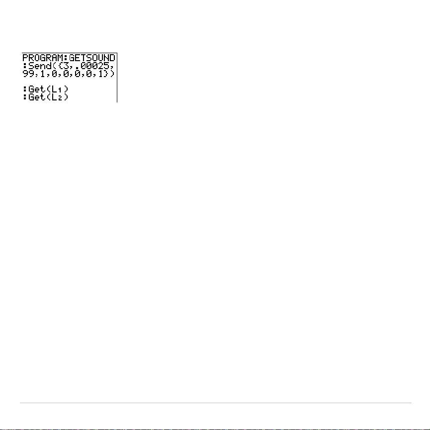
TI-83 Plus Programming 534
Send(
variable
)
Note: This program gets sound
data and time in seconds from
CBL 2/CBL.
Note: You can access
Get(
,
Send(
, and
GetCalc(
from the
CATALOG
to execute
them from the home screen (Chapter 15).

TI-83 Plus Programming 535
Calling Other Programs as Subroutines
Calling a Program from Another Program
On the TI-83 Plus, any stored program can be called from another
program as a subroutine. Enter the name of the program to use as a
subroutine on a line by itself.
You can enter a program name on a command line in either of two ways.
•
Press
|
to display the
PRGM EXEC
menu and select the name of
the program
prgm
name
is pasted to the current cursor location on a
command line.
•
Select
prgm
from the
PRGM CTL
menu, and then enter the program
name.
prgm
name
When
prgm
name
is encountered during execution, the next command that
the program executes is the first command in the second program. It
returns to the subsequent command in the first program when it
encounters either
Return
or the implied
Return
at the end of the second
program.
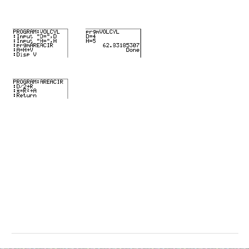
TI-83 Plus Programming 536
Program Output
&
Subroutine
(
'
Notes about Calling Programs
Variables are global.
label
used with
Goto
and
Lbl
is local to the program where it is located.
label
in one program is not recognized by another program. You cannot
use
Goto
to branch to a
label
in another program.
Return
exits a subroutine and returns to the calling program, even if it is
encountered within nested loops.

TI-83 Plus Programming 537
Running an Assembly Language Program
You can run programs written for the TI-83 Plus in assembly language.
Typically, assembly language programs run much faster and provide
greater control than than the keystroke programs that you write with the
built-in program editor.
Note:
Because an assembly langauge program has greater control over the
calculator, if your assembly language program has error(s), it may cause your
calculator to reset and lose all data, programs, and applications stored in
memory.
When you download an assembly language program, it is stored among
the other programs as a
PRGM
menu item. You can:
•
Transmit it using the TI-83 Plus communication link (Chapter 19).
•
Delete it using the
MEM MGMT
DEL
screen (Chapter 18).
To run an assembly Program, the syntax is:
Asm(
assemblyprgmname
)
If you write an assembly language program, use the two instructions below
from the
CATALOG
to identify and compile the program.

TI-83 Plus Programming 538
Instructions Comments
AsmComp(
prgmASM1,
p
rgmASM2
)
Compiles an assembly language program written in
ASCII and stores the hex version
AsmPrgm
Identifies an assembly language program; must be
entered as the first line of an assembly language
program
To compile an assembly program that you have written:
1. Follow the steps for writing a program (16-4) but be sure to include
AsmPrgm
as the first line of your program.
2. From the home screen, press
y
N
and then select
AsmComp(
to paste it to the screen
3. Press
to display the
PRGM EXEC
menu.
4. Select the program you want to compile. It will be pasted to the home
screen.
5. Press
¢
and then select
prgm
from the
CATALOG
6. Key in the name you have chosen for the output program.
Note: This name must be unique — not a copy of an existing program
name.

TI-83 Plus Programming 539
7. Press
¤
to complete the sequence.
The sequence of the arguments should be as follows:
AsmComp(
prgmASM1,
prgmASM2
)
8. Press
Í
to compile your program and generate the output
program.

TI-83 Plus Activities 540
Chapter 17:
Activities
The Quadratic Formula
Entering a Calculation
Use the quadratic formula to solve the quadratic equations 3X
2
+ 5X + 2 = 0 and
2X
2
N
X + 3 = 0. Begin with the equation 3X
2
+ 5X + 2 = 0.
1. Press
3
¿
ƒ
[
A
] (above
) to store
the coefficient of the X
2
term.
2. Press
ƒ
[
:
] (above
Ë
). The colon allows
you to enter more than one instruction on a line.
3. Press
5
¿
ƒ
[
B
] (above
Œ
) to store
the coefficient of the X term. Press
ƒ
[
:
] to
enter a new instruction on the same line. Press
2
¿
ƒ
[
C
] (above
) to store the
constant.
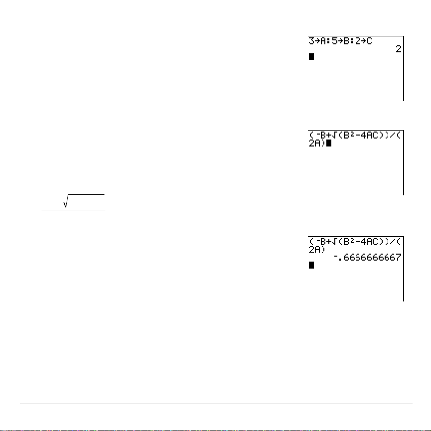
TI-83 Plus Activities 541
4. Press
Í
to store the values to the variables
A, B, and C.
The last value you stored is shown on the right
side of the display. The cursor moves to the
next line, ready for your next entry.
5. Press
£
Ì
ƒ
[
B
]
Ã
y
C
ƒ
[
B
]
¡
¹
4
ƒ
[
A
]
ƒ
[
C
]
¤
¤
¥
£
2
ƒ
[
A
]
¤
to enter the expression for one of the
solutions for the quadratic formula,
a
acbb
2
4
2
−±−
6. Press
Í
to find one solution for the
equation 3X
2
+ 5X + 2 = 0.
The answer is shown on the right side of the
display. The cursor moves to the next line,
ready for you to enter the next expression.
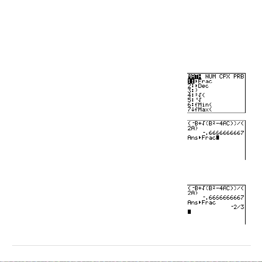
TI-83 Plus Activities 542
The Quadratic Formula
Converting to a Fraction
You can show the solution as a fraction.
1. Press
to display the
MATH
menu.
2. Press
1
to select
1:
4
Frac
from the
MATH
menu.
When you press
1
,
Ans
4
Frac
is displayed on the
home screen.
Ans
is a variable that contains the
last calculated answer.
3. Press
Í
to convert the result to a fraction.
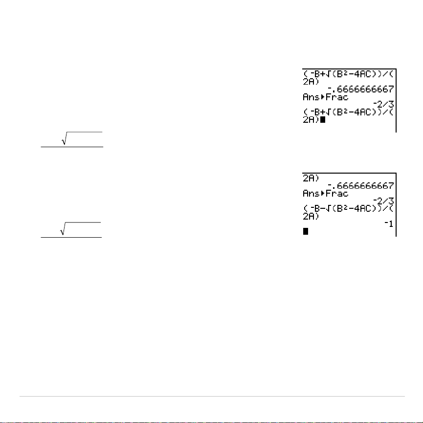
TI-83 Plus Activities 543
To save keystrokes, you can recall the last expression you entered, and
then edit it for a new calculation.
4. Press
y
[
(above
Í
) to recall the
fraction conversion entry, and then press
y
[
again to recall the quadratic-formula
expression,
a
acbb
2
4
2
−+−
5. Press
}
to move the cursor onto the
+
sign in
the formula. Press
¹
to edit the quadratic-
formula expression to become:
a
acbb
2
4
2
−−
−
6. Press
Í
to find the other solution for the
quadratic equation 3X
2
+ 5X + 2 = 0.
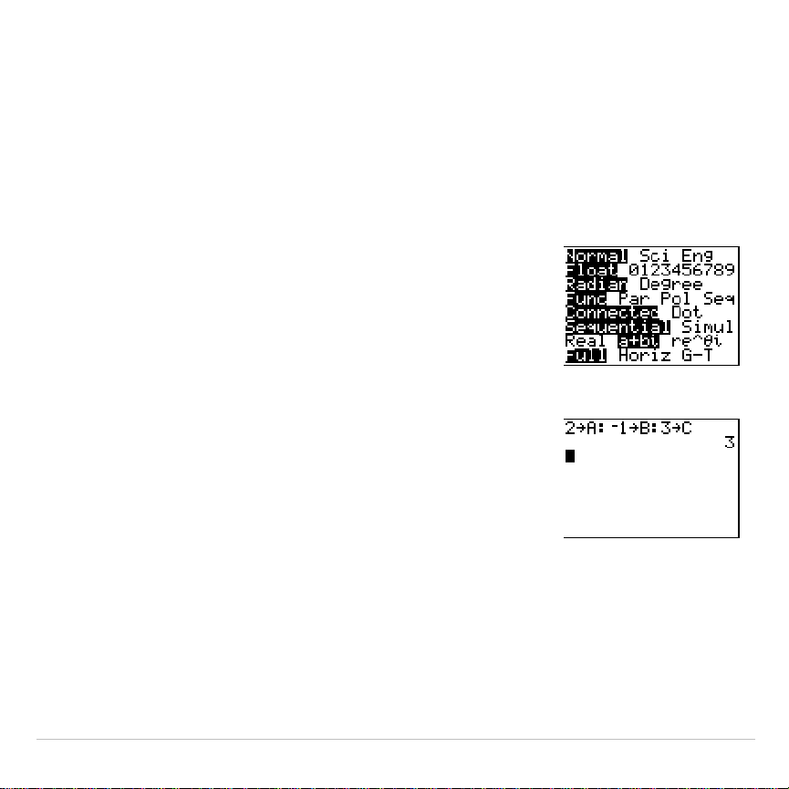
TI-83 Plus Activities 544
The Quadratic Formula
Displaying Complex Results
Now solve the equation 2X
2
N
X + 3 = 0. When you set
a+b
i
complex
number mode, the TI-83 Plus displays complex results.
1. Press
z
†
†
†
†
†
†
(6 times), and
then press
~
to position the cursor over
a+b
i
.
Press
Í
to select
a+b
i
complex-number
mode.
2. Press
y
5
(above
z
) to return to the
home screen, and then press
‘
to clear it.
3. Press
2
¿
ƒ
[
A
]
ƒ
[
:
]
Ì
1
¿
ƒ
[
B
]
ƒ
[
:
]
3
¿
ƒ
[
C
]
Í
.
The coefficient of the X
2
term, the coefficient of
the X term, and the constant for the new
equation are stored to A, B, and C, respectively.
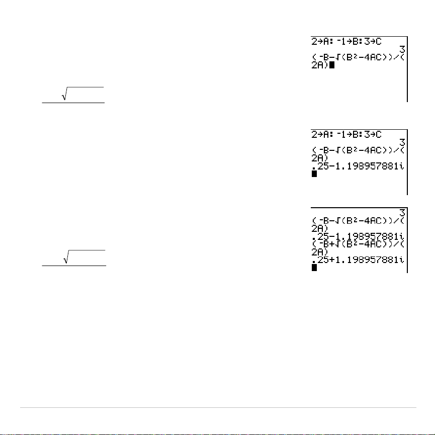
TI-83 Plus Activities 545
4. Press
y
[
to recall the store instruction,
and then press
y
[
again to recall the
quadratic-formula expression,
a
acbb
2
4
2
−−
−
5. Press
Í
to find one solution for the
equation 2X
2
N
X + 3 = 0.
6. Press
y
[
repeatedly until this quadratic-
formula expression is displayed:
a
acbb
2
4
2
−+−
7. Press
Í
to find the other solution for the
quadratic equation: 2X
2
N
X + 3 = 0.
Note:
An alternative for solving equations for real numbers is to use the built-in
Equation Solver (Chapter 2).
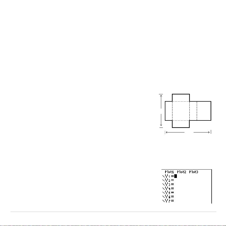
TI-83 Plus Activities 546
Box with Lid
Defining a Function
Take a 20 cm × 25 cm. sheet of paper and cut X × X squares from two
corners. Cut X × 12.5 cm rectangles from the other two corners as
shown in the diagram below. Fold the paper into a box with a lid. What
value of X would give your box the maximum volume V? Use the table
and graphs to determine the solution.
Begin by defining a function that describes the
volume of the box.
From the diagram: 2X + A = 20
2X + 2B = 25
V = A*B*X
Substituting: V = (20
N
2X) (25
à
2
N
X) X
1. Press
o
to display the
Y=
editor, which is
where you define functions for tables and
graphing.
A2
0
X
X B X B
25
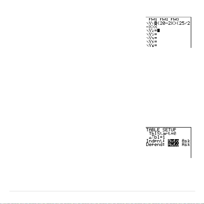
TI-83 Plus Activities 547
2. Press
£
20
¹
2
„
¤
£
25
¥
2
¹
„
¤
„
Í
to define the volume function
as
Y1
in terms of
X
.
„
lets you enter
X
quickly, without having
to press
ƒ
. The highlighted
=
sign indicates
that
Y1
is selected.
Box with Lid
Defining a Table of Values
The table feature of the TI-83 Plus displays numeric information about a
function. You can use a table of values from the function you just defined
to estimate an answer to the problem.
1. Press
y
-
(above
p
) to display the
TABLE SETUP
menu.
2. Press
Í
to accept
TblStart=0
.
3. Press
1
Í
to define the table increment
@
Tbl=1
. Leave
Indpnt: Auto
and
Depend: Auto
so
that the table will be generated automatically.
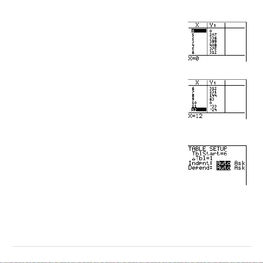
TI-83 Plus Activities 548
4. Press
y
0
(above
s
) to display the
table.
Notice that the maximum value for
Y1
(box’s
volume) occurs when
X
is about
4
, between
3
and
5
.
5. Press and hold
†
to scroll the table until a
negative result for
Y1
is displayed.
Notice that the maximum length of
X
for this
problem occurs where the sign of
Y1
(box’s
volume) changes from positive to negative,
between
10
and
11
.
6. Press
y
-
.
Notice that
TblStart
has changed to
6
to reflect
the first line of the table as it was last displayed.
(In step 5, the first value of
X
displayed in the
table is
6
.)
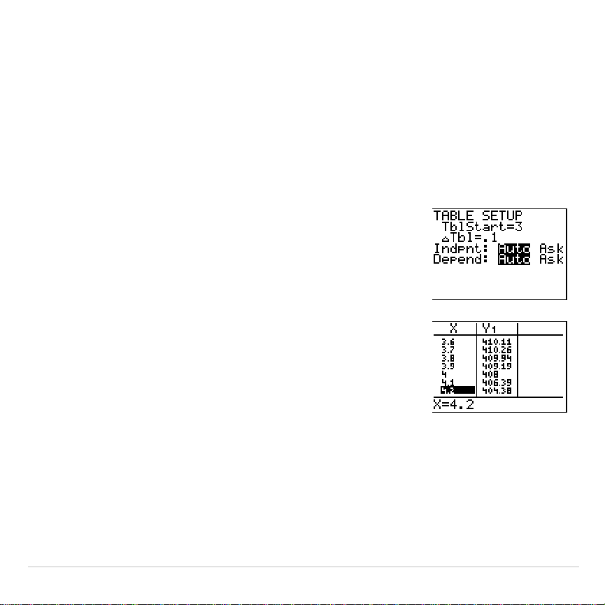
TI-83 Plus Activities 549
Box with Lid
Zooming In on the Table
You can adjust the way a table is displayed to get more information
about a defined function. With smaller values for
@
Tbl
, you can zoom in
on the table.
1. Press
3
Í
to set
TblStart
. Press
Ë
1
Í
to set
@
Tbl
.
This adjusts the table setup to get a more
accurate estimate of
X
for maximum volume
Y1
.
2. Press
y
0
.
3. Press
†
and
}
to scroll the table.
Notice that the maximum value for
Y1
is
410.26
,
which occurs at
X
=
3.7
. Therefore, the maximum
occurs where
3.6
<
X
<
3.8
.
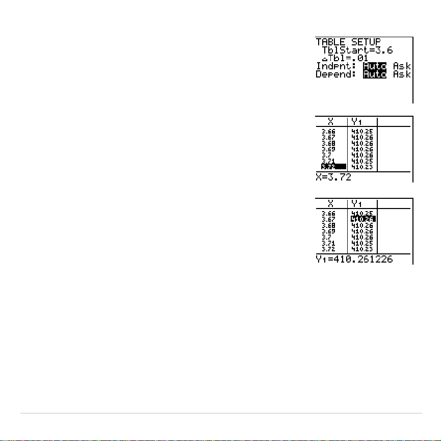
TI-83 Plus Activities 550
4. Press
y
-
. Press
3
Ë
6
Í
to set
TblStart
. Press
Ë
01
Í
to set
@
Tbl
.
5. Press
y
0
, and then press
†
and
}
to
scroll the table.
Four equivalent maximum values are shown,
410.26
at
X
=
3.67
,
3.68
,
3.69
, and
3.70
.
6. Press
†
or
}
to move the cursor to
3.67
. Press
~
to move the cursor into the
Y1
column.
The value of
Y1
at
X
=
3.67
is displayed on the
bottom line in full precision as
410.261226
.
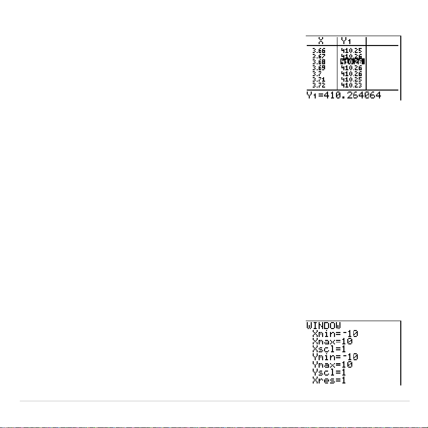
TI-83 Plus Activities 551
7. Press
†
to display the other maximum.
The value of
Y1
at
X
=
3.68
in full precision is
410.264064
, at
X
=
3.69
is
410.262318
and at
X
=
3.7
is
410.256
.
The maximum volume of the box would occur at
3.68
if you could measure and cut the paper at
.01-centimeter increments.
Box with Lid
Setting the Viewing Window
You also can use the graphing features of the TI-83 Plus to find the
maximum value of a previously defined function. When the graph is
activated, the viewing window defines the displayed portion of the
coordinate plane. The values of the window variables determine the size
of the viewing window.
1. Press
p
to display the window editor,
where you can view and edit the values of the
window variables.
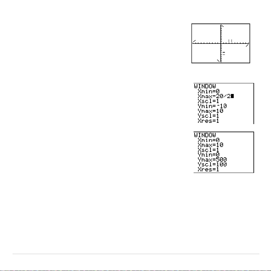
TI-83 Plus Activities 552
The standard window variables define the
viewing window as shown.
Xmin
,
Xmax
,
Ymin
,
and
Ymax
define the boundaries of the display.
Xscl
and
Yscl
define the distance between tick
marks on the
X
and
Y
axes.
Xres
controls
resolution.
Xmax
Ymin
Ymax
Xscl
Yscl
Xmin
2. Press
0
Í
to define
Xmin
.
3. Press
20
¥
2
to define
Xmax
using an
expression.
4. Press
Í
. The expression is evaluated, and
10
is stored in
Xmax
. Press
Í
to accept
Xscl
as
1
.
5. Press
0
Í
500
Í
100
Í
1
Í
to
define the remaining window variables.
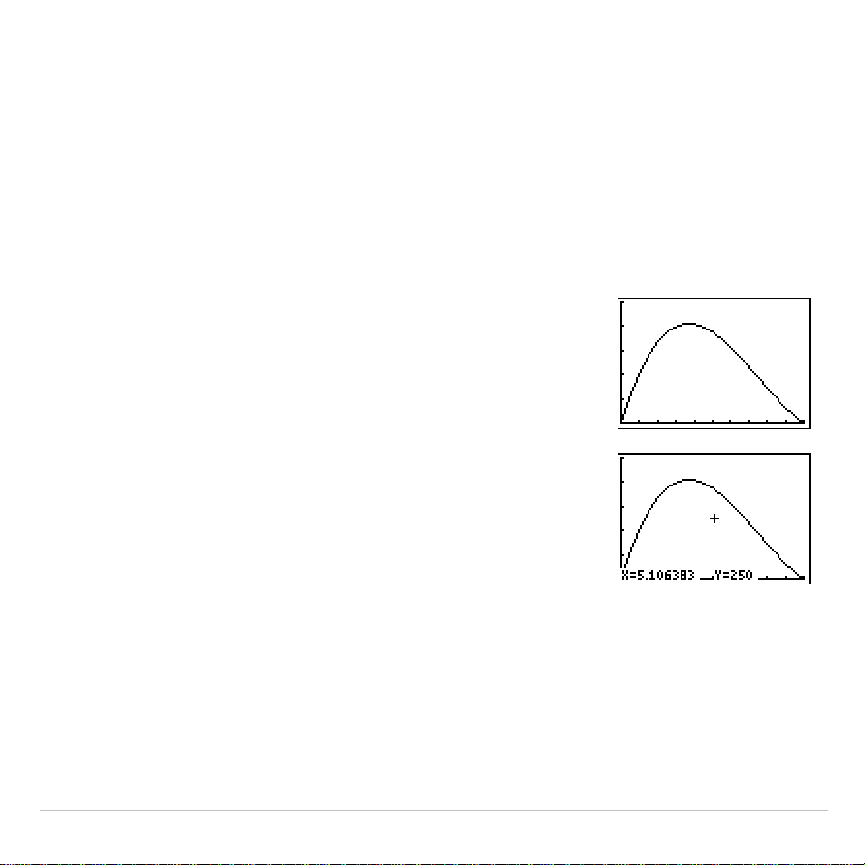
TI-83 Plus Activities 553
Box with Lid
Displaying and Tracing the Graph
Now that you have defined the function to be graphed and the window in
which to graph it, you can display and explore the graph. You can trace
along a function using the
TRACE
feature.
1. Press
s
to graph the selected function in
the viewing window.
The graph of
Y1=(20
N
2X)(25
à
2
N
X)X
is displayed.
2. Press
~
to activate the free-moving graph
cursor.
The
X
and
Y
coordinate values for the position
of the graph cursor are displayed on the bottom
line.
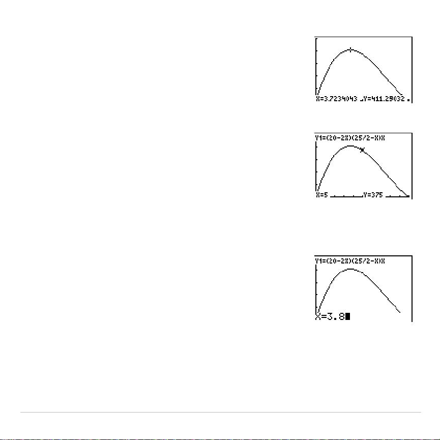
TI-83 Plus Activities 554
3. Press
|
,
~
,
}
, and
†
to move the free-
moving cursor to the apparent maximum of the
function.
As you move the cursor, the
X
and
Y
coordinate
values are updated continually.
4. Press
r
. The trace cursor is displayed on
the
Y1
function.
The function that you are tracing is displayed in
the top-left corner.
5. Press
|
and
~
to trace along
Y1
, one
X
dot at
a time, evaluating
Y1
at each
X
.
You also can enter your estimate for the
maximum value of
X
.
6. Press
3
Ë
8
. When you press a number key
while in
TRACE
, the
X=
prompt is displayed in the
bottom-left corner.
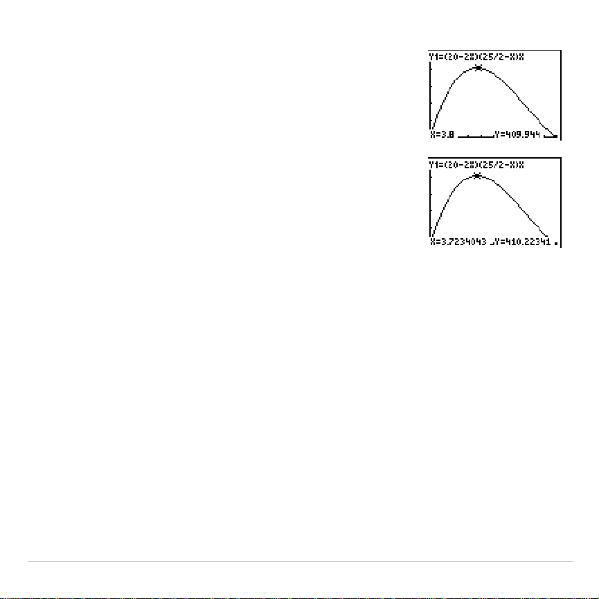
TI-83 Plus Activities 555
7. Press
Í
.
The trace cursor jumps to the point on the
Y1
function evaluated at
X=3.8
.
8. Press
|
and
~
until you are on the maximum
Y
value.
This is the maximum of
Y1(X)
for the
X
pixel
values. The actual, precise maximum may lie
between pixel values.
Box with Lid
Zooming In on the Graph
To help identify maximums, minimums, roots, and intersections of
functions, you can magnify the viewing window at a specific location
using the
ZOOM
instructions.
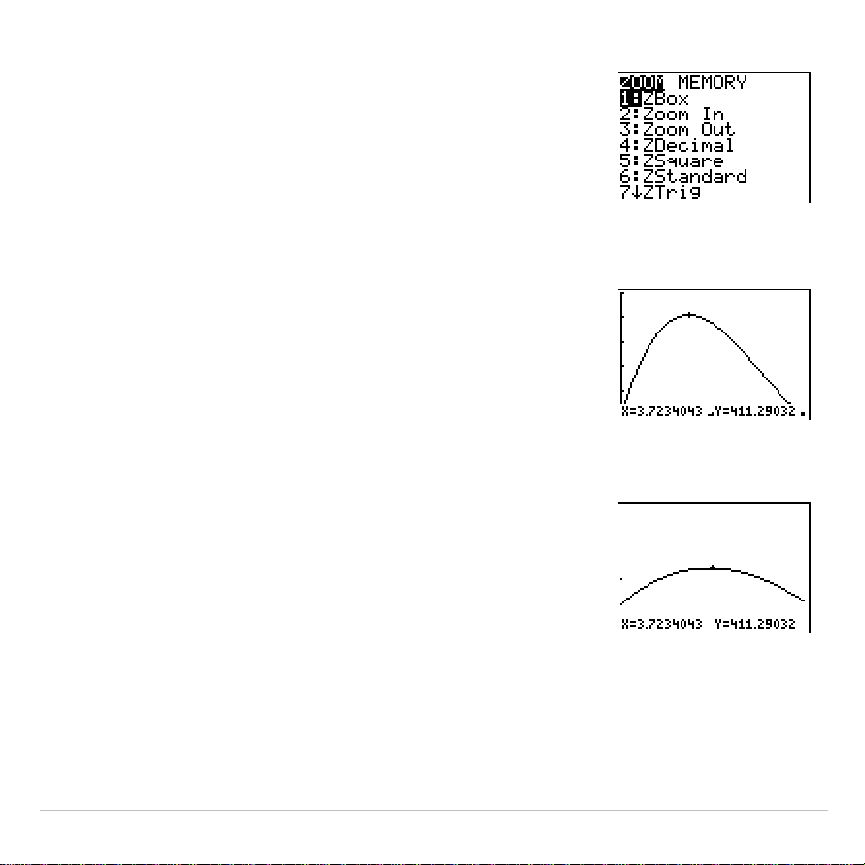
TI-83 Plus Activities 556
1. Press
q
to display the
ZOOM
menu.
This menu is a typical TI-83 Plus menu. To
select an item, you can either press the number
or letter next to the item, or you can press
†
until the item number or letter is highlighted,
and then press
Í
.
2. Press
2
to select
2:Zoom In
.
The graph is displayed again. The cursor has
changed to indicate that you are using a
ZOOM
instruction.
3. With the cursor near the maximum value of the
function, press
Í
.
The new viewing window is displayed. Both
Xmax
N
Xmin
and
Ymax
N
Ymin
have been
adjusted by factors of 4, the default values for
the zoom factors.
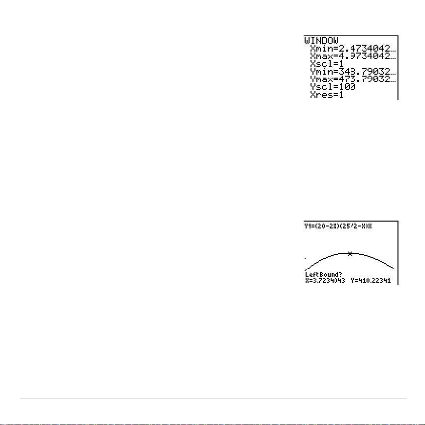
TI-83 Plus Activities 557
4. Press
p
to display the new window
settings.
Box with Lid
Finding the Calculated Maximum
You can use a
CALCULATE
menu operation to calculate a local maximum
of a function.
1. Press
y
/
(above
r
) to display the
CALCULATE
menu. Press
4
to select
4:maximum
.
The graph is displayed again with a
Left Bound?
prompt.
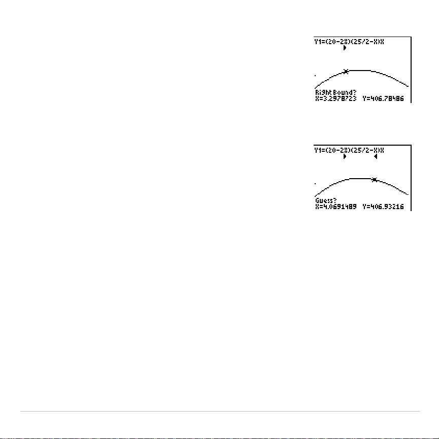
TI-83 Plus Activities 558
2. Press
|
to trace along the curve to a point to
the left of the maximum, and then press
Í
.
A
4
at the top of the screen indicates the
selected bound.
A
Right Bound?
prompt is displayed.
3. Press
~
to trace along the curve to a point to
the right of the maximum, and then press
Í
.
A
3
at the top of the screen indicates the
selected bound.
A
Guess?
prompt is displayed.
4. Press
|
to trace to a point near the maximum,
and then press
Í
.
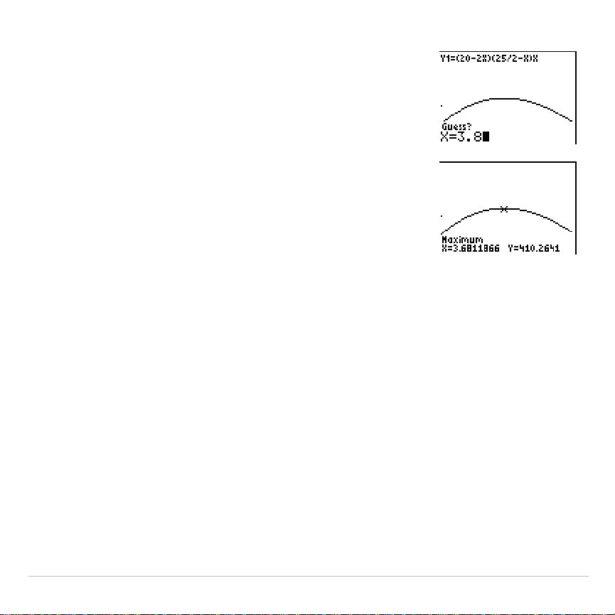
TI-83 Plus Activities 559
Or, press
3
Ë
8
, and then press
Í
to enter
a guess for the maximum.
When you press a number key in
TRACE
, the
X=
prompt is displayed in the bottom-left corner.
Notice how the values for the calculated
maximum compare with the maximums found
with the free-moving cursor, the trace cursor,
and the table.
Note: In steps 2 and 3 above, you can enter values
directly for Left Bound and Right Bound, in the same
way as described in step 4.

TI-83 Plus Activities 560
Comparing Test Results Using Box Plots
Problem
An experiment found a significant difference between boys and girls
pertaining to their ability to identify objects held in their left hands, which
are controlled by the right side of their brains, versus their right hands,
which are controlled by the left side of their brains. The TI Graphics team
conducted a similar test for adult men and women.
The test involved 30 small objects, which participants were not allowed to
see. First, they held 15 of the objects one by one in their left hands and
guessed what they were. Then they held the other 15 objects one by one
in their right hands and guessed what they were. Use box plots to
compare visually the correct-guess data from this table.
Correct Guesses
Women
Left
Women
Right
Men
Left
Men
Right
84712
9186
12 8 7 12
11 12 5 12
10 11 7 7
811811

TI-83 Plus Activities 561
Women
Left
Women
Right
Men
Left
Men
Right
12 13 11 12
7124 8
9111012
11 12 14 11
13 9
59
Procedure
1. Press
…
5
to select
5:SetUpEditor
. Enter list names
WLEFT
,
WRGHT
,
MLEFT
, and
MRGHT
, separated by commas. Press
Í
.
The stat list editor now contains only these four lists.
2. Press
…
1
to select
1:Edit
.
3. Enter into
WLEFT
the number of correct guesses each woman made
using her left hand (
Women Left
). Press
~
to move to
WRGHT
and enter
the number of correct guesses each woman made using her right hand
(
Women Right
).
4. Likewise, enter each man’s correct guesses in
MLEFT
(
Men Left
)
and
MRGHT
(
Men Right
).
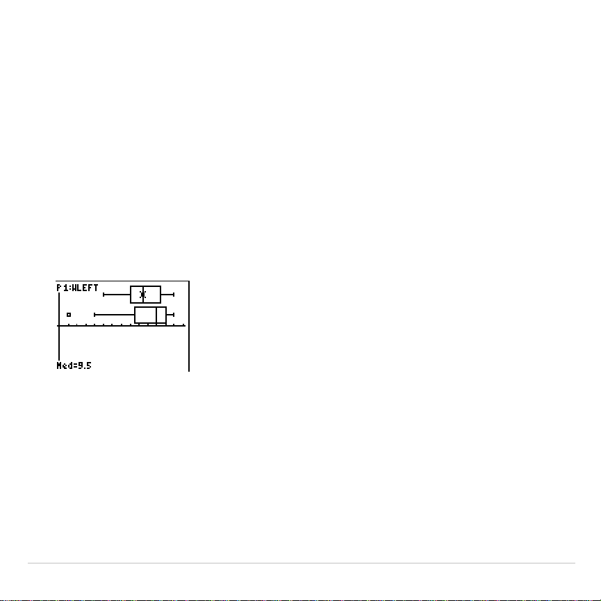
TI-83 Plus Activities 562
5. Press
y
,
. Select
1:Plot1
. Turn on plot 1; define it as a
modified box plot
Õ
that uses
WLEFT
. Move the cursor to the top line
and select
Plot2
. Turn on plot 2; define it as a modified box plot that
uses
WRGHT
.
6. Press
o
. Turn off all functions.
7. Press
p
. Set
Xscl=1
and
Yscl=0
. Press
q
9
to select
9:ZoomStat
. This adjusts the viewing window and displays the box
plots for the women’s results.
8. Press
r
.
% Women’s left-hand data
% Women’s right-hand data
Use
|
and
~
to examine
minX
,
Q1
,
Med
,
Q3
, and
maxX
for each plot.
Notice the outlier to the women’s right-hand data. What is the median
for the left hand? For the right hand? With which hand were the
women more accurate guessers, according to the box plots?
9. Examine the men’s results. Redefine plot 1 to use
MLEFT
, redefine
plot 2 to use
MRGHT
. Press
r
.
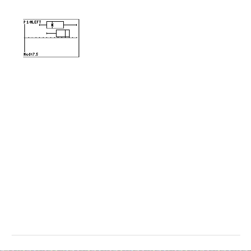
TI-83 Plus Activities 563
% Men’s left-hand data
% Men’s right-hand data
Press
|
and
~
to examine
minX
,
Q1
,
Med
,
Q3
, and
maxX
for each
plot. What difference do you see between the plots?
10.Compare the left-hand results. Redefine plot 1 to use
WLEFT
,
redefine plot 2 to use
MLEFT
, and then press
r
to examine
minX
,
Q1
,
Med
,
Q3
, and
maxX
for each plot. Who were the better left-hand
guessers, men or women?
11.Compare the right-hand results. Define plot 1 to use
WRGHT
, define plot
2 to use
MRGHT
, and then press
r
to examine
minX
,
Q1
,
Med
,
Q3
,
and
maxX
for each plot. Who were the better right-hand guessers?
In the original experiment boys did not guess as well with right hands,
while girls guessed equally well with either hand. This is not what our
box plots show for adults. Do you think that this is because adults
have learned to adapt or because our sample was not large enough?

TI-83 Plus Activities 564
Graphing Piecewise Functions
Problem
The fine for speeding on a road with a speed limit of 45 kilometers per
hour (kph) is 50; plus 5 for each kph from 46 to 55 kph; plus 10 for each
kph from 56 to 65 kph; plus 20 for each kph from 66 kph and above.
Graph the piecewise function that describes the cost of the ticket.
The fine (Y) as a function of kilometers per hour (X) is:
Y = 0 0 < X
45
Y = 50 + 5 (X
N
45) 45 < X
55
Y = 50 + 5
ä
10 + 10 (X
N
55) 55 < X
65
Y = 50 + 5
ä
10 + 10
ä
10 + 20 (X
N
65) 65 < X
Procedure
1. Press
z
. Select
Func
and the default settings.
2. Press
o
. Turn off all functions and stat plots. Enter the
Y=
function to
describe the fine. Use the
TEST
menu operations to define the
piecewise function. Set the graph style for
Y1
to
í
(dot).
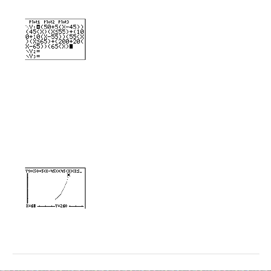
TI-83 Plus Activities 565
3. Press
p
and set
Xmin=
L
2
,
Xscl=10
,
Ymin=
L
5
, and
Yscl=10
. Ignore
Xmax
and
Ymax
; they are set by
@
X
and
@
Y
in step 4.
4. Press
y
5
to return to the home screen. Store
1
to
@
X
, and then
store
5
to
@
Y
.
@
X
and
@
Y
are on the
VARS Window X/Y
secondary menu.
@
X
and
@
Y
specify the horizontal and vertical distance between the
centers of adjacent pixels. Integer values for
@
X
and
@
Y
produce nice
values for tracing.
5. Press
r
to plot the function. At what speed does the ticket
exceed 250?
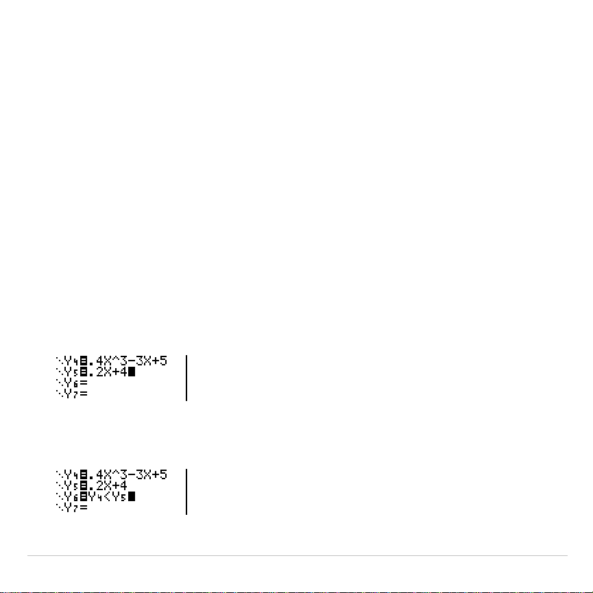
TI-83 Plus Activities 566
Graphing Inequalities
Problem
Graph the inequality 0
.
4X
3
N
3X + 5 < 0
.
2X + 4. Use the
TEST
menu
operations to explore the values of X where the inequality is true and
where it is false.
Procedure
1. Press
z
. Select
Dot
,
Simul
, and the default settings. Setting
Dot
mode changes all graph style icons to
í
(dot) in the
Y=
editor.
2. Press
o
. Turn off all functions and stat plots. Enter the left side of the
inequality as
Y4
and the right side as
Y5
.
3. Enter the statement of the inequality as
Y6
. This function evaluates to
1
if true or
0
if false.
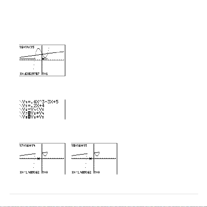
TI-83 Plus Activities 567
4. Press
q
6
to graph the inequality in the standard window.
5. Press
r
†
†
to move to
Y6
. Then press
|
and
~
to trace the
inequality, observing the value of
Y
.
6. Press
o
. Turn off
Y4
,
Y5
, and
Y6
. Enter equations to graph only the
inequality.
7. Press
r
. Notice that the values of
Y7
and
Y8
are zero where the
inequality is false.
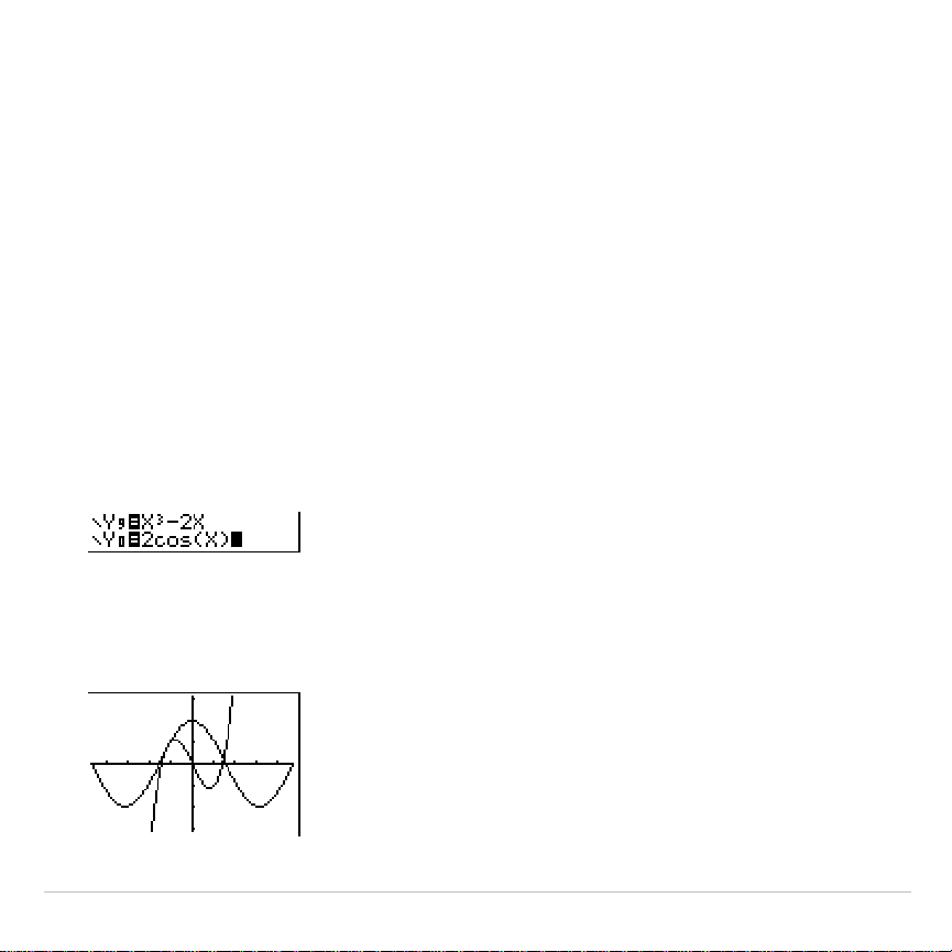
TI-83 Plus Activities 568
Solving a System of Nonlinear Equations
Problem
Using a graph, solve the equation X
3
N
2X = 2cos(X). Stated another
way, solve the system of two equations and two unknowns: Y = X
3
N
2X
and Y = 2cos(X). Use
ZOOM
factors to control the decimal places
displayed on the graph.
Procedure
1. Press
z
. Select the default mode settings. Press
o
. Turn off all
functions and stat plots. Enter the functions.
2. Press
q
4
to select
4:ZDecimal
. The display shows that two
solutions may exist (points where the two functions appear to
intersect).

TI-83 Plus Activities 569
3. Press
q
~
4
to select
4:SetFactors
from the
ZOOM MEMORY
menu.
Set
XFact=10
and
YFact=10
.
4. Press
q
2
to select
2:Zoom In
. Use
|
,
~
,
}
, and
†
to move the
free-moving cursor onto the apparent intersection of the functions on
the right side of the display. As you move the cursor, notice that the
X
and
Y
values have one decimal place.
5. Press
Í
to zoom in. Move the cursor over the intersection. As
you move the cursor, notice that now the
X
and
Y
values have two
decimal places.
6. Press
Í
to zoom in again. Move the free-moving cursor onto a
point exactly on the intersection. Notice the number of decimal
places.
7. Press
y
/
5
to select
5:intersect
. Press
Í
to select the first
curve and
Í
to select the second curve. To guess, move the
trace cursor near the intersection. Press
Í
. What are the
coordinates of the intersection point?
8. Press
q
4
to select
4:ZDecimal
to redisplay the original graph.
9. Press
q
. Select
2:Zoom In
and repeat steps 4 through 8 to explore
the apparent function intersection on the left side of the display.
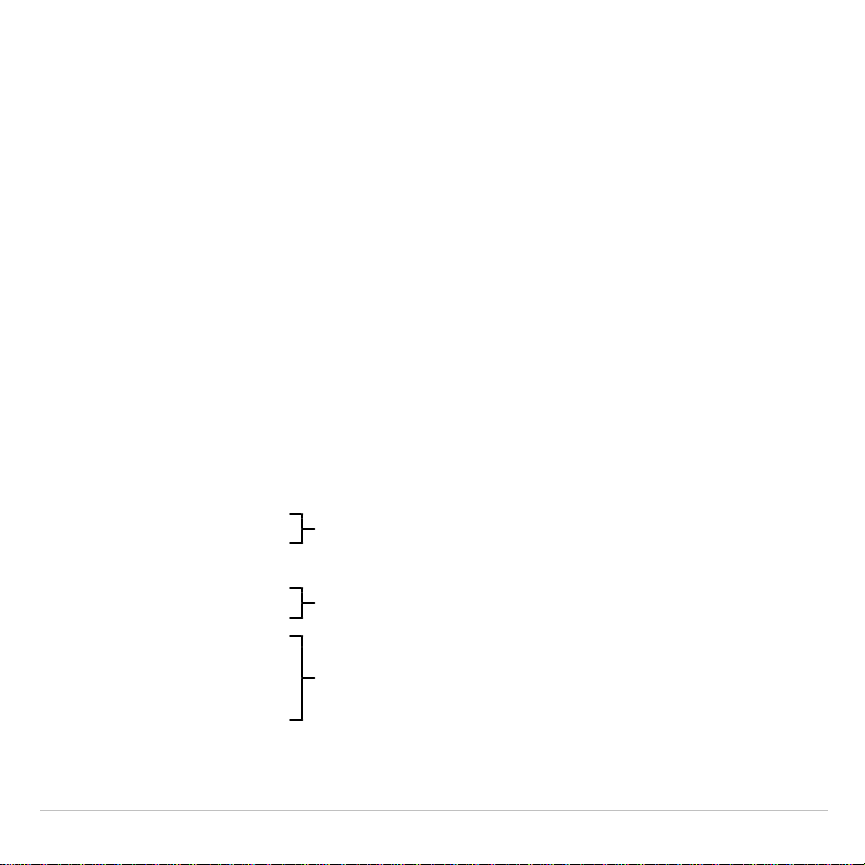
TI-83 Plus Activities 570
Using a Program to Create the Sierpinski
Triangle
Setting up the Program
This program creates a drawing of a famous fractal, the Sierpinski
Triangle, and stores the drawing to a picture. To begin, press
~
~
1
. Name the program
SIERPINS
, and then press
Í
. The program
editor is displayed.
Program
PROGRAM:SIERPINS
:FnOff :ClrDraw
:PlotsOff
:AxesOff
:0!Xmin:1!Xmax
:0!Ymin:1!Ymax
Set viewing window.
:rand!X:rand!Y
:For(K,1,3000)
:rand!N
Beginning of
For
group.
:If N
1
à
3
:Then
:.5X!X
:.5Y!Y
:End
If
/
Then
group
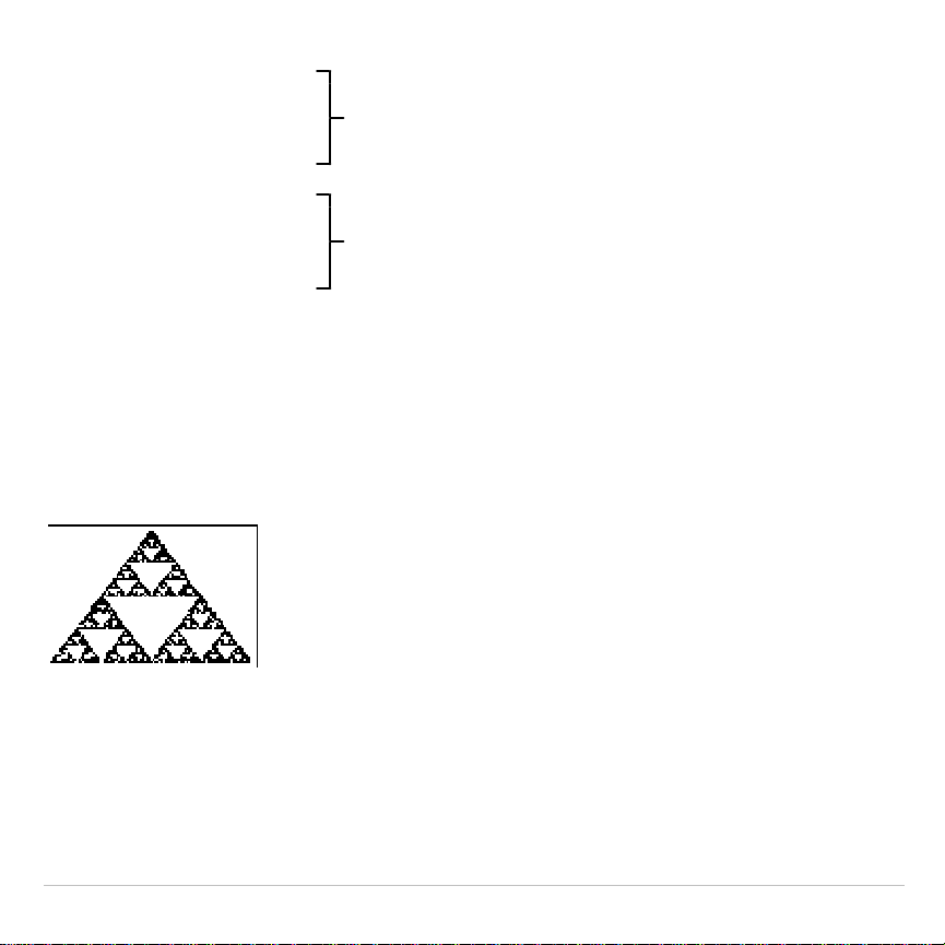
TI-83 Plus Activities 571
:If 1
à
3<N and N
2
à
3
:Then
:.5(.5+X)!X
:.5(1+Y)!Y
:End
If
/
Then
group.
:If 2
à
3<N
:Then
:.5(1+X)!X
:.5Y!Y
:End
If
/
Then
group.
:Pt-On(X,Y)
Draw point.
:End
End of
For
group.
:StorePic 6
Store picture.
After you execute the program above, you can recall and display the
picture with the instruction
RecallPic 6
.

TI-83 Plus Activities 572
Graphing Cobweb Attractors
Problem
Using
Web
format, you can identify points with attracting and repelling
behavior in sequence graphing.
Procedure
1. Press
z
. Select
Seq
and the default mode settings. Press
y
.
. Select
Web
format and the default format settings.
2. Press
o
. Clear all functions and turn off all stat plots. Enter the
sequence that corresponds to the expression Y = K X(1
N
X).
u(
n
)=Ku(
n
N
1)(1
N
u(
n
N
1))
u(
n
Min)=.01
3. Press
y
5
to return to the home screen, and then store
2.9
to
K
.
4. Press
p
. Set the window variables.
n
Min=0 Xmin=0 Ymin=
M
.26
n
Max=10 Xmax=1 Ymax=1.1
PlotStart=1 Xscl=1 Yscl=1
PlotStep=1
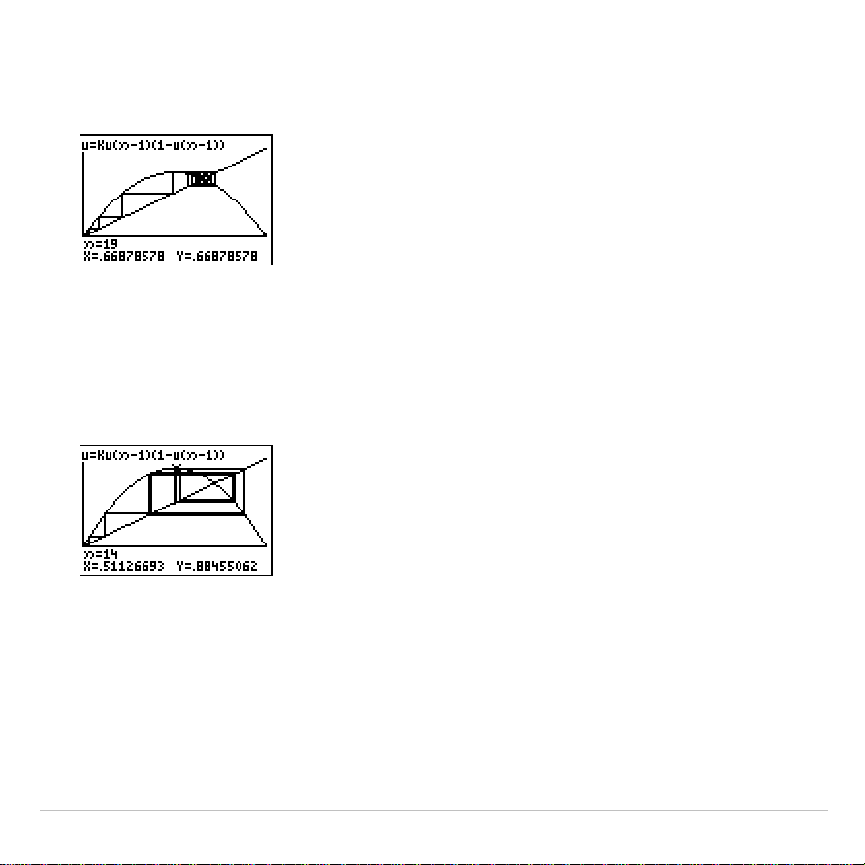
TI-83 Plus Activities 573
5. Press
r
to display the graph, and then press
~
to trace the
cobweb. This is a cobweb with one attractor.
6. Change
K
to
3.44
and trace the graph to show a cobweb with two
attractors.
7. Change
K
to
3.54
and trace the graph to show a cobweb with four
attractors.
TI-83 Plus Activities 574
Using a Program to Guess the Coefficients
Setting Up the Program
This program graphs the function A sin(BX) with random integer
coefficients between 1 and 10. Try to guess the coefficients and graph
your guess as C sin(DX). The program continues until your guess is
correct.
Program
PROGRAM:GUESS
:PlotsOff :Func
:FnOff :Radian
:ClrHome
:"Asin(BX)"!Y1
:"Csin(DX)"!Y2
Define equations.
:GraphStyle(1,1)
:GraphStyle(2,5)
Set line and path graph styles.
:FnOff 2
:randInt(1,10)!A
:randInt(1,10)!B
:0!C:0!D
Initialize coefficients.
:
L
2
p!Xmin
:2
p!Xmax
:
pà
2!Xscl
:
L
10!Ymin
:10!Ymax
Set viewing window.
TI-83 Plus Activities 575
:1!Yscl
:DispGraph
:Pause
Display graph.
:FnOn 2
:Lbl Z
:Prompt C,D
Prompt for guess.
:DispGraph
:Pause
Display graph.
:If C=A
:Text(1,1,"C IS OK")
:If C
ƒ
A
:Text(1,1,"C IS WRONG")
:If D=B
:Text(1,50,"D IS OK")
:If D
ƒ
B
:Text(1,50,"D IS WRONG")
Display results.
:DispGraph
:Pause
Display graph.
:If C=A and D=B
:Stop
:Goto Z
Quit if guesses are correct.

TI-83 Plus Activities 576
Graphing the Unit Circle and Trigonometric
Curves
Problem
Using parametric graphing mode, graph the unit circle and the sine curve
to show the relationship between them.
Any function that can be plotted in
Func
mode can be plotted in
Par
mode
by defining the
X
component as
T
and the
Y
component as
F(T)
.
Procedure
1. Press
z
. Select
Par
,
Simul
, and the default settings.
2. Press
p
. Set the viewing window.
Tmin=0 Xmin=
L
2 Ymin=
L
3
Tmax=2
p
Xmax=7.4 Ymax=3
Tstep=.1 Xscl=
pà
2 Yscl=1
3. Press
o
. Turn off all functions and stat plots. Enter the expressions
to define the unit circle centered on (0,0).
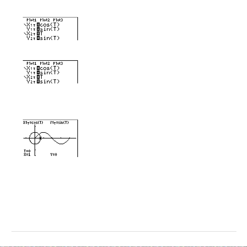
TI-83 Plus Activities 577
4. Enter the expressions to define the sine curve.
5. Press
r
. As the graph is plotting, you may press
Í
to pause
and
Í
again to resume graphing as you watch the sine function
“unwrap” from the unit circle.
Note:
You can generalize the unwrapping. Replace
sin(T)
in
Y
2
T
with any other
trig function to unwrap that function.

TI-83 Plus Activities 578
Finding the Area between Curves
Problem
Find the area of the region bounded by
f(x) = 300x/(x
2
+ 625)
g(x)= 3cos(
.
1x)
x=75
Procedure
1. Press
z
. Select the default mode settings.
2. Press
p
. Set the viewing window.
Xmin=0 Ymin=
L
5
Xmax=100 Ymax=10
Xscl=10 Yscl=1
Xres=1
3. Press
o
. Turn off all functions and stat plots. Enter the upper and
lower functions.
Y1=300X
à
(X
2
+625)
Y
2=3cos(.1X)
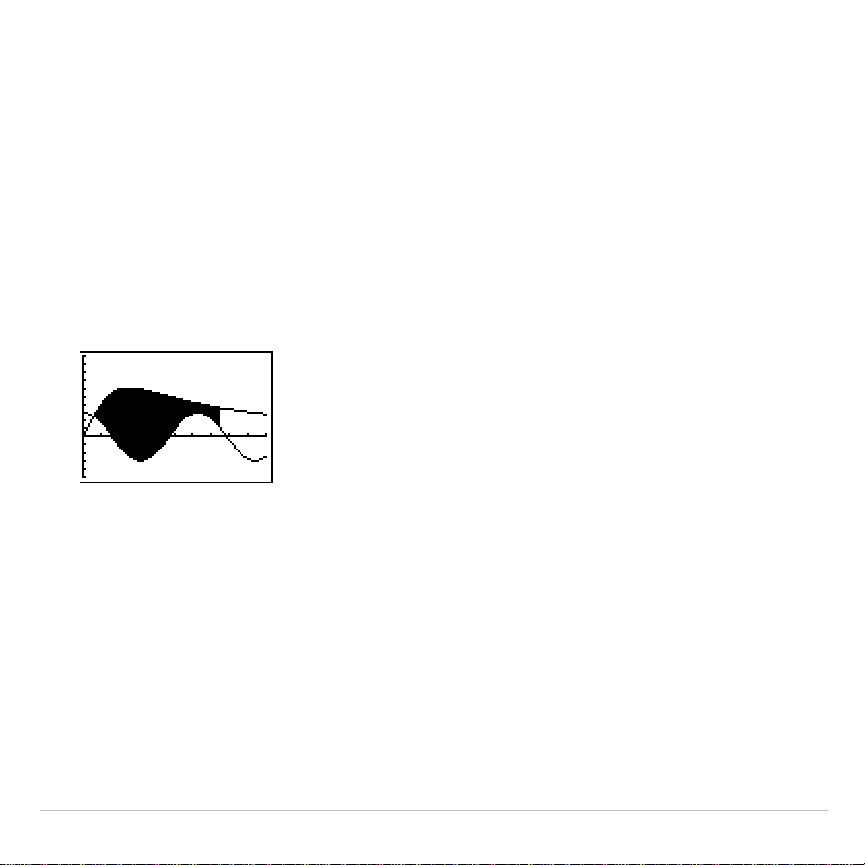
TI-83 Plus Activities 579
4. Press
y
/
5
to select
5:Intersect
. The graph is displayed. Select
a first curve, second curve, and guess for the intersection toward the
left side of the display. The solution is displayed, and the value of
X
at
the intersection, which is the lower limit of the integral, is stored in
Ans
and
X
.
5. Press
y
5
to go to the home screen. Press
y
<
7
and use
Shade(
to see the area graphically.
Shade(Y2,Y1,Ans,75)
6. Press
y
5
to return to the home screen. Enter the expression to
evaluate the integral for the shaded region.
fnInt(Y1–Y2,X,Ans,75)
The area is
325.839962
.

TI-83 Plus Activities 580
Using Parametric Equations: Ferris Wheel
Problem
Problem
Using two pairs of parametric equations, determine when two objects in
motion are closest to each other in the same plane.
A ferris wheel has a diameter (d) of 20 meters and is rotating
counterclockwise at a rate (s) of one revolution every 12 seconds. The
parametric equations below describe the location of a ferris wheel
passenger at time T, where
a
is the angle of rotation, (0,0) is the bottom
center of the ferris wheel, and (10,10) is the passenger’s location at the
rightmost point, when T=0.
X(T) = r cos
a
where
a
= 2
p
Ts and r = d
à
2
Y(T) = r + r sin
a
A person standing on the ground throws a ball to the ferris wheel
passenger. The thrower’s arm is at the same height as the bottom of the
ferris wheel, but 25 meters (b) to the right of the ferris wheel’s lowest point
(25,0). The person throws the ball with velocity (v
0
) of 22 meters per
second at an angle (
q
) of 66
¡
from the horizontal. The parametric
equations below describe the location of the ball at time T.
X(T) = b
N
Tv
0
cos
q
Y(T) = Tv
0
sin
q
N
(g
à
2) T
2
where g = 9.8 m/sec
2
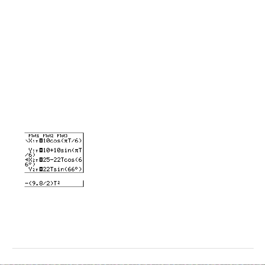
TI-83 Plus Activities 581
Procedure
1. Press
z
. Select
Par
,
Simul
, and the default settings.
Simul
(simultaneous) mode simulates the two objects in motion over time.
2. Press
p
. Set the viewing window.
Tmin=0 Xmin=
L
13 Ymin=0
Tmax=12 Xmax=34 Ymax=31
Tstep=.1 Xscl=10 Yscl=10
3. Press
o
. Turn off all functions and stat plots. Enter the expressions to
define the path of the ferris wheel and the path of the ball. Set the
graph style for
X2T
to
ë
(path).
Tip: Try setting the graph styles to
ë
X
1T
and
ì
X
2T
, which simulates a chair on
the ferris wheel and the ball flying through the air when you press
s
.
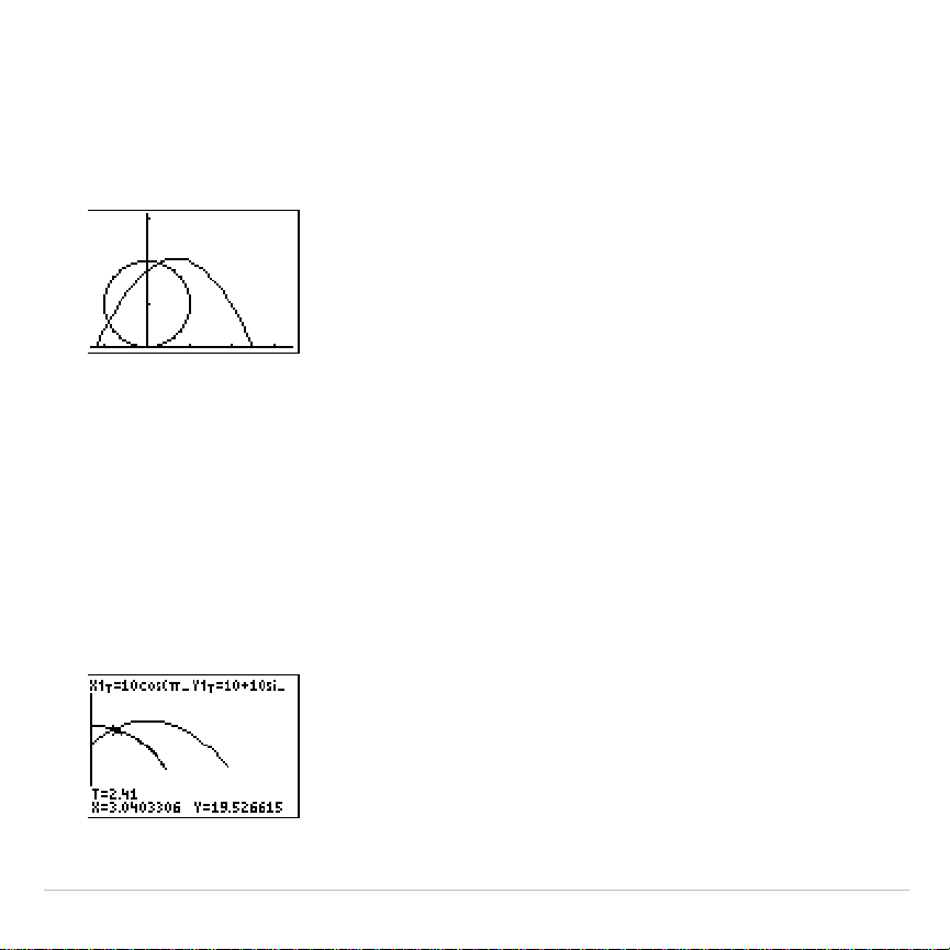
TI-83 Plus Activities 582
4. Press
s
to graph the equations. Watch closely as they are
plotted. Notice that the ball and the ferris wheel passenger appear to
be closest where the paths cross in the top-right quadrant of the ferris
wheel.
5. Press
p
. Change the viewing window to concentrate on this
portion of the graph.
Tmin=1 Xmin=0 Ymin=10
Tmax=3 Xmax=23.5 Ymax=25.5
Tstep=.03 Xscl=10 Yscl=10
6. Press
r
. After the graph is plotted, press
~
to move near the
point on the ferris wheel where the paths cross. Notice the values of
X
,
Y
, and
T
.
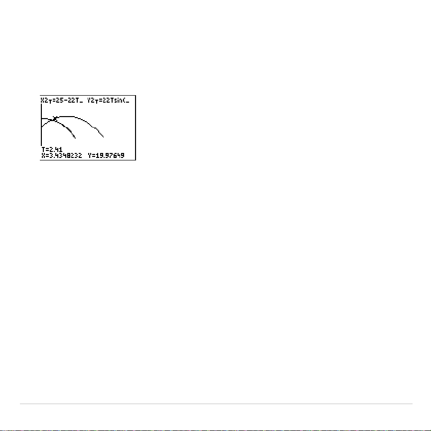
TI-83 Plus Activities 583
7. Press
†
to move to the path of the ball. Notice the values of
X
and
Y
(
T
is unchanged). Notice where the cursor is located. This is the
position of the ball when the ferris wheel passenger passes the
intersection. Did the ball or the passenger reach the intersection first?
You can use
r
to, in effect, take snapshots in time and explore
the relative behavior of two objects in motion.

TI-83 Plus Activities 584
Demonstrating the Fundamental Theorem of
Calculus
Problem 1
Using the functions
fnInt(
and
nDeriv(
from the
MATH
menu to graph
functions defined by integrals and derivatives demonstrates graphically
that:
∫
>==
x
xxdtxF
1
0),(ln)(
and that
x
dt
t
Dx
x
1
1
1
=
∫
Procedure 1
1. Press
z
. Select the default settings.
2. Press
p
. Set the viewing window.
Xmin=.01 Ymin=
M
1.5 Xres=3
Xmax=10 Ymax=2.5
Xscl=1 Yscl=1
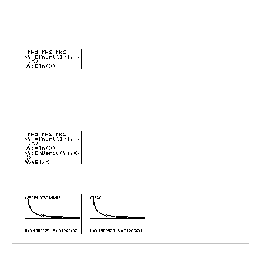
TI-83 Plus Activities 585
3. Press
o
. Turn off all functions and stat plots. Enter the numerical
integral of 1
à
T from 1 to X and the function ln(X). Set the graph style
for
Y1
to
ç
(line) and
Y2
to
ë
(path).
4. Press
r
. Press
|
,
}
,
~
, and
†
to compare the values of
Y1
and
Y2
.
5. Press
o
. Turn off
Y1
and
Y2
, and then enter the numerical derivative
of the integral of 1
à
X and the function 1
à
X. Set the graph style for
Y3
to
ç
(line) and
Y4
to
è
(thick).
6. Press
r
. Again, use the cursor keys to compare the values of the
two graphed functions,
Y3
and
Y4
.
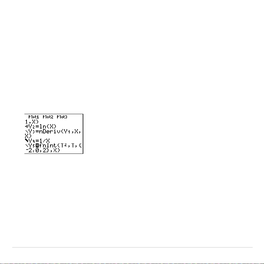
TI-83 Plus Activities 586
Problem 2
Explore the functions defined by
∫∫∫
=
xxx
dttdttdtty
2
2
0
2
2
2
,and,,
Procedure 2
1. Press
o
. Turn off all functions and stat plots. Use a list to define
these three functions simultaneously. Store the function in
Y5.
2. Press
q
6
to select
6:ZStandard
.
3. Press
r
. Notice that the functions appear identical, only shifted
vertically by a constant.
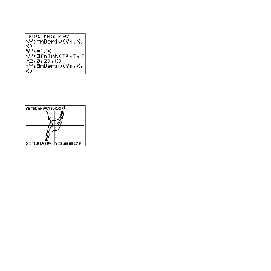
TI-83 Plus Activities 587
4. Press
o
. Enter the numerical derivative of
Y5
in
Y6
.
5. Press
r
. Notice that although the three graphs defined by
Y5
are
different, they share the same derivative.
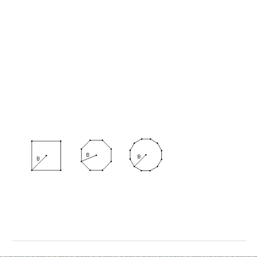
TI-83 Plus Activities 588
Computing Areas of Regular N-Sided
Polygons
Problem
Use the equation solver to store a formula for the area of a regular
N-sided polygon, and then solve for each variable, given the other
variables. Explore the fact that the limiting case is the area of a circle,
p
r
2
.
Consider the formula A = NB
2
sin(
pà
N) cos(
pà
N) for the area of a
regular polygon with N sides of equal length and B distance from the
center to a vertex.
N = 4 sides N = 8 sides N = 12 sides
Procedure
1. Press
0
to select
0:Solver
from the
MATH
menu. Either the
equation editor or the interactive solver editor is displayed. If the
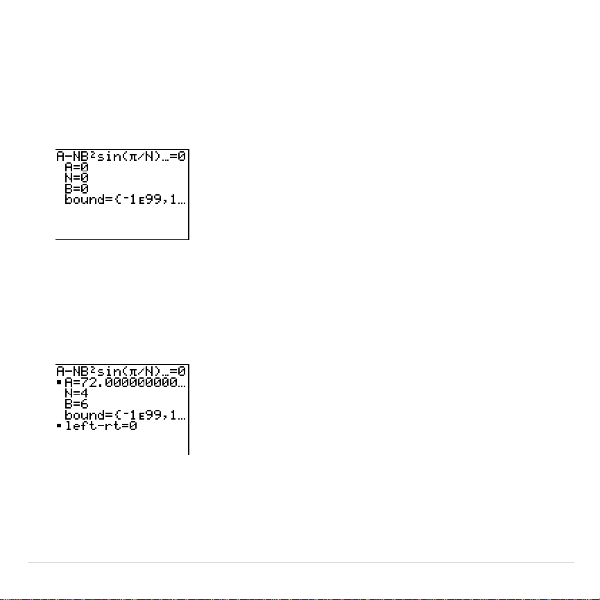
TI-83 Plus Activities 589
interactive solver editor is displayed, press
}
to display the equation
editor.
2. Enter the formula as
0=A
N
NB
2
sin(
p
/ N)cos(
p
/ N)
, and then press
Í
. The interactive solver editor is displayed.
3. Enter
N=4
and
B=6
to find the area (
A
) of a square with a distance (
B
)
from center to vertex of 6 centimeters.
4. Press
}
}
to move the cursor onto
A
, and then press
ƒ
\
.
The solution for
A
is displayed on the interactive solver editor.
5. Now solve for
B
for a given area with various number of sides. Enter
A=200
and
N=6
. To find the distance
B
, move the cursor onto
B
, and
then press
ƒ
\
.

TI-83 Plus Activities 590
6. Enter
N=8
. To find the distance
B
, move the cursor onto
B
, and then
press
ƒ
\
. Find
B
for
N=9
, and then for
N=10
.
Find the area given
B=6
, and
N=10
,
100
,
150
,
1000
, and
10000
. Compare
your results with
p
6
2
(the area of a circle with radius 6), which is
approximately 113.097.
7. Enter
B=6
. To find the area
A
, move the cursor onto
A
, and then press
ƒ
\
. Find
A
for
N=10
, then
N=100
, then
N=150
, then
N=1000
,
and finally
N=10000
. Notice that as
N
gets large, the area
A
approaches
p
B
2
.
Now graph the equation to see visually how the area changes as the
number of sides gets large.
8. Press
z
. Select the default mode settings.
9. Press
p
. Set the viewing window.
Xmin=0 Ymin=0 Xres=1
Xmax=200 Ymax=150
Xscl=10 Yscl=10
10.Press
o
. Turn off all functions and stat plots. Enter the equation for
the area. Use
X
in place of
N
. Set the graph styles as shown.
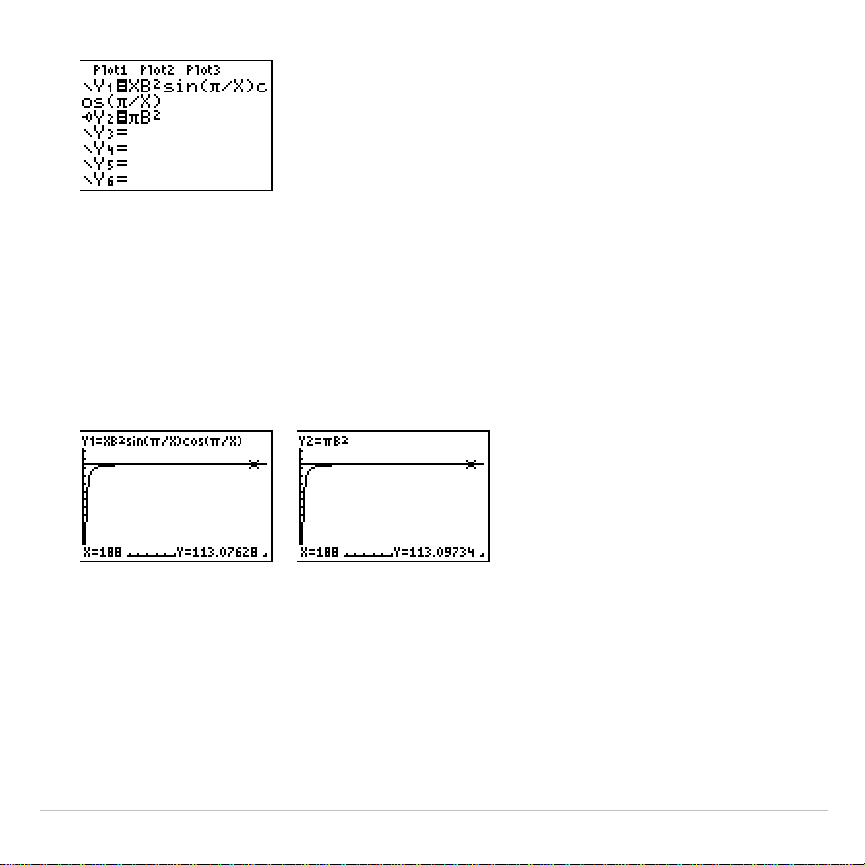
TI-83 Plus Activities 591
11.Press
r
. After the graph is plotted, press
100
Í
to trace to
X=100
. Press
150
Í
. Press
188
Í
. Notice that as
X
increases,
the value of
Y
converges to
p
6
2
, which is approximately 113.097.
Y2=
p
B
2
(the area of the circle) is a horizontal asymptote to
Y1
. The
area of an N-sided regular polygon, with r as the distance from the
center to a vertex, approaches the area of a circle with radius r (
p
r
2
)
as N gets large.
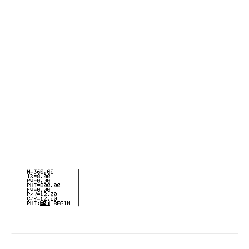
TI-83 Plus Activities 592
Computing and Graphing Mortgage
Payments
Problem
You are a loan officer at a mortgage company, and you recently closed
on a 30-year home mortgage at 8 percent interest with monthly
payments of 800. The new home owners want to know how much will be
applied to the interest and how much will be applied to the principal
when they make the 240th payment 20 years from now.
Procedure
1. Press
z
and set the fixed-decimal mode to
2
decimal places. Set
the other mode settings to the defaults.
2. Press
Œ
Í
Í
to display the
TVM Solver
. Enter these values.
Note: Enter a positive number (
800
) to show
PMT
as a cash inflow. Payment
values will be displayed as positive numbers on the graph. Enter
0
for
FV
,

TI-83 Plus Activities 593
since the future value of a loan is 0 once it is paid in full. Enter
PMT: END
,
since payment is due at the end of a period.
3. Move the cursor onto the
PV=
prompt, and then press
ƒ
\
.
The present value, or mortgage amount, of the house is displayed at
the
PV=
prompt.
Now compare the graph of the amount of interest with the graph of the
amount of principal for each payment.
4. Press
z
. Set
Par
and
Simul
.
5. Press
o
. Turn off all functions and stat plots. Enter these equations
and set the graph styles as shown.
Note:
G
Prn(
and
G
Int(
are located on the
FINANCE menu
(
APPS 1:FINANCE
).
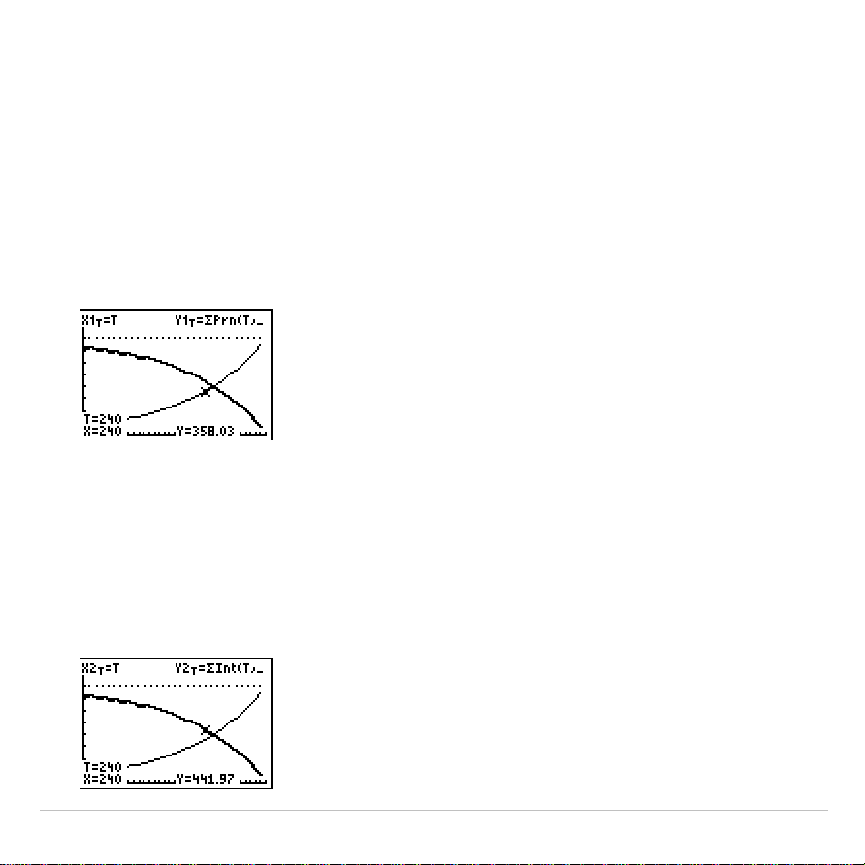
TI-83 Plus Activities 594
6. Press
p
. Set these window variables.
Tmin=1 Xmin=0 Ymin=0
Tmax=360 Xmax=360 Ymax=1000
Tstep=12 Xscl=10 Yscl=100
Tip: To increase the graph speed, change
Tstep
to
24
.
7. Press
r
. After the graph is drawn, press
240
Í
to move the
trace cursor to
T=240
, which is equivalent to 20 years of payments.
The graph shows that for the 240th payment (
X=240
), 358.03 of the
800 payment is applied to principal (
Y=358.03
).
Note: The sum of the payments (
Y3T=Y1T+Y2T
) is always 800.
8. Press
†
to move the cursor onto the function for interest defined by
X2T
and
Y2T
. Enter
240
.
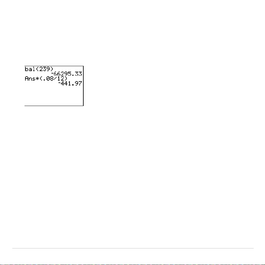
TI-83 Plus Activities 595
The graph shows that for the 240th payment (
X=240
), 441.97 of the
800 payment is interest (
Y=441.97
).
9. Press
y
5
Œ
Í
9
to paste
9:bal(
to the home screen.
Check the figures from the graph.
At which monthly payment will the principal allocation surpass the
interest allocation?

TI-83 Plus Memory and Variable Management 596
Chapter 18:
Memory and Variable Management
Checking Available Memory
MEMORY Menu
At any time you can check available memory or manage existing
memory by selecting items from the
MEMORY
menu. To access this menu,
press
y
L
.
MEMORY
1:About
...
Displays information about the calculator.
2:Mem Mgmt/Del
...
Reports memory availability and variable usage.
3:Clear Entries
Clears
ENTRY
(last-entry storage).
4:ClrAllLists
Clears all lists in memory.
5:Archive
...
Archives a selected variable.
6:UnArchive
...
UnArchives a selected variable.
7:Reset
...
Displays the
RAM
,
ARCHIVE
, and
ALL
menus
8:Group
...
Displays
GROUP
and
UNGROUP
menus.
To check
memory usage
, first press
y
L
and then press
2:Mem
Mgmt/Del
.
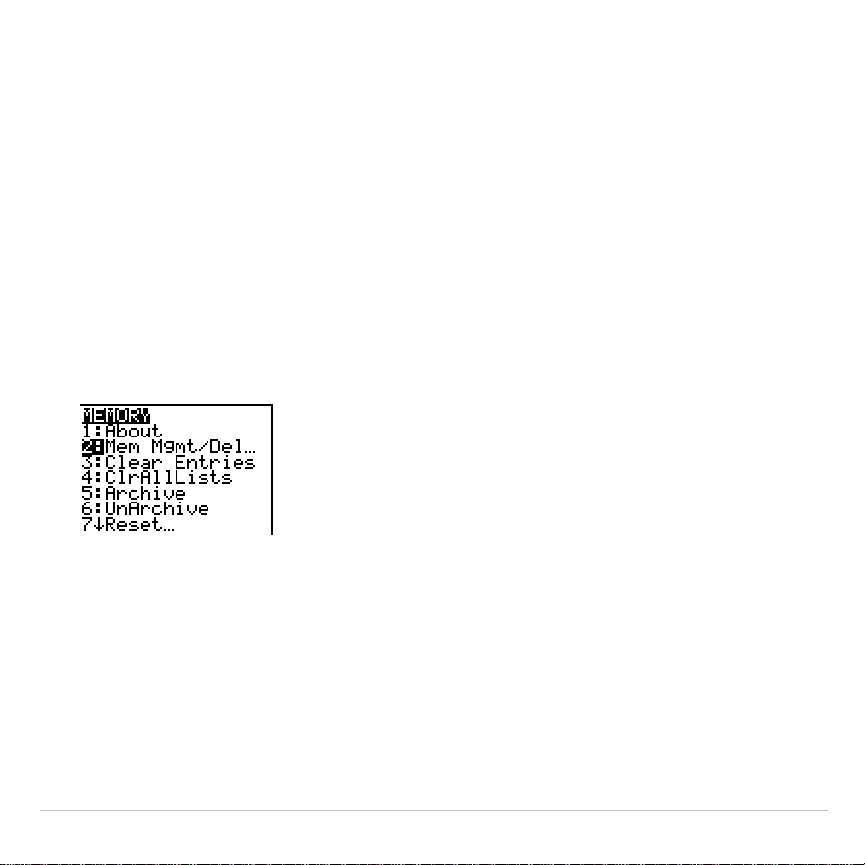
TI-83 Plus Memory and Variable Management 597
Displaying the
MEMORY MANAGEMENT/DELETE Menu
Mem Mgmt/Del
displays the
MEMORY MANAGEMENT/DELETE
menu. The two
lines at the top report the total amount of available
RAM
and
ARCHIVE
memory. By selecting menu items on this screen, you can see the
amount of memory each variable type is using. This information can help
you determine if some variables need to be deleted from memory to
make room for new data, such as programs or applications.
To check memory usage, follow these steps.
1. Press
y
L
to display the
MEMORY
menu.
Note: The
#
and
$
in the top or bottom
of the left column indicate that you can
scroll up or down to view more
variable types.
2. Select
2:Mem Mgmt/Del
to display the
MEMORY MANAGEMENT/DELETE
menu. The TI-83 Plus expresses memory quantities in bytes.
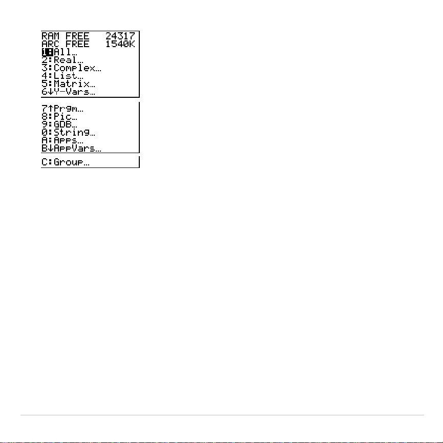
TI-83 Plus Memory and Variable Management 598
3. Select variable types from the list
to display memory usage.
Note:
Real
,
List
,
Y
.
Vars
, and
Prgm
variable types never reset to zero, even
after memory is cleared.
Apps
are independent applications which are stored in Flash ROM.
AppVars
is a variable holder used to store variables created by independent
applications. You cannot edit or change variables in
AppVars
unless you do
so through the application which created them.
To leave the
MEMORY MANAGEMENT/DELETE
menu, press either
y
5
or
‘
. Both options display the home screen.
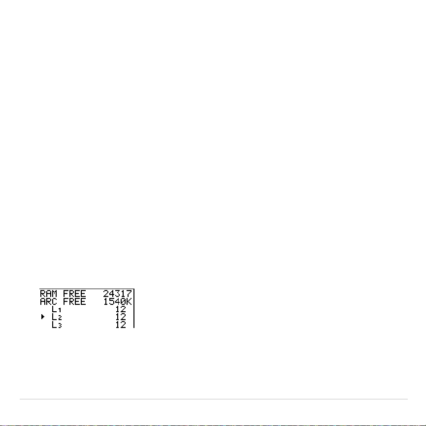
TI-83 Plus Memory and Variable Management 599
Deleting Items from Memory
Deleting an Item
To increase available memory by deleting the contents of any variable
(real or complex number, list, matrix,
Y=
variable, program, Apps,
AppVars, picture, graph database, or string), follow these steps.
1. Press
y
L
to display the
MEMORY
menu.
2. Select
2:Mem Mgmt/Del
to display the
MEMORY MANAGEMENT/DELETE
menu.
3. Select the type of data you want to delete, or select
1:All
for a list of
all variables of all types. A screen is displayed listing each variable of
the type you selected and the number of bytes each variable is using.
For example, if you select
4:List
, the
LIST
editor screen is displayed.

TI-83 Plus Memory and Variable Management 600
4. Press
}
and
†
to move the selection cursor (
4
) next to the item you
want to delete, and then press
{
. The variable is deleted from
memory. You can delete individual variables one by one from this
screen.
Note:
If you are deleting programs or Apps, you will receive a message
asking you to confirm this delete action. Select
2:Yes
to continue.
To leave any variable screen without deleting anything, press
y
5
, which displays the home screen.
Note:
You cannot delete some system variables, such as the last-answer
variable
Ans
and the statistical variable
RegEQ
.
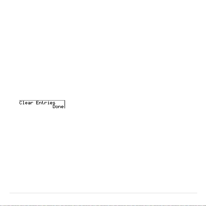
TI-83 Plus Memory and Variable Management 601
Clearing Entries and List Elements
Clear Entries
Clear Entries
clears the contents of the
ENTRY
(last entry) storage area
(Chapter 1). To clear the
ENTRY
storage area, follow these steps.
1. Press
y
L
to display the
MEMORY
menu.
2. Select
3:Clear Entries
to paste the instruction to the home screen.
3. Press
Í
to clear the
ENTRY
storage area.
To cancel
Clear Entries
, press
‘
.
Note: If you select
3:Clear Entries
from within a program, the
Clear Entries
instruction is pasted to the program editor, and the
Entry
(last entry) is cleared
when the program is executed.
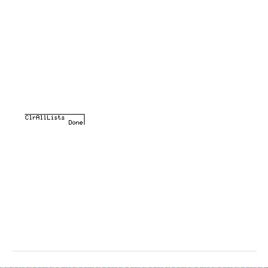
TI-83 Plus Memory and Variable Management 602
ClrAllLists
ClrAllLists
sets the dimension of each list in RAM only to
0
.
To clear all elements from all lists, follow these steps.
1. Press
y
L
to display the
MEMORY
menu.
2. Select
4:ClrAllLists
to paste the instruction to the home screen.
3. Press
Í
to set to
0
the dimension of each list in memory.
To cancel
ClrAllLists
, press
‘
.
ClrAllLists
does not delete list names from memory, from the
LIST NAMES
menu, or from the stat list editor.
Note: If you select
4:ClrAllLists
from within a program, the
ClrAllLists
instruction
is pasted to the program editor. The lists are cleared when the program is
executed.

TI-83 Plus Memory and Variable Management 603
Resetting the TI-83 Plus
RAM ARCHIVE ALL Menu
The
RAM ARCHIVE ALL
menu gives you the option of resetting all
memory (including default settings) or resetting selected portions of
memory while preserving other data stored in memory, such as
programs and
Y=
functions. For instance, you can choose to reset all of
RAM or just restore the default settings. Be aware that if you choose to
reset RAM, all data and programs in RAM will be erased. For archive
memory, you can reset variables (Vars), applications (Apps), or both of
these. Be aware that if you choose to reset Vars, all data and programs
in archive memory will be erased. If you choose to reset Apps, all
applications in archive memory will be erased.
When you reset defaults on the TI-83 Plus, all defaults in RAM are
restored to the factory settings. Stored data and programs are not
changed.
These are some examples of TI-83 Plus defaults that are restored by
resetting the defaults.
•
Mode settings such as
Normal
(notation);
Func
(graphing);
Real
(numbers); and
Full
(screen)
•
Y=
functions off
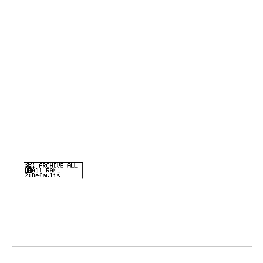
TI-83 Plus Memory and Variable Management 604
•
Window variable values such as
Xmin=
L
10
;
Xmax=10
;
Xscl=1
;
Yscl=1
;
and
Xres=1
•
Stat plots off
•
Format settings such as
CoordOn
(graphing coordinates on);
AxesOn
;
and
ExprOn
(expression on)
•
rand
seed value to 0
Displaying the RAM ARCHIVE ALL Menu
To display the
RAM ARCHIVE ALL
menu on the TI-83 Plus, follow these
steps.
1. Press
y
L
to display the
MEMORY
menu.
2. Select
7:Reset
to display the
RAM ARCHIVE ALL
menu.
Resetting RAM Memory
Resetting RAM restores RAM system variables to factory settings and
deletes all nonsystem variables and all programs. Resetting defaults
restores all system variables to default settings without deleting variables
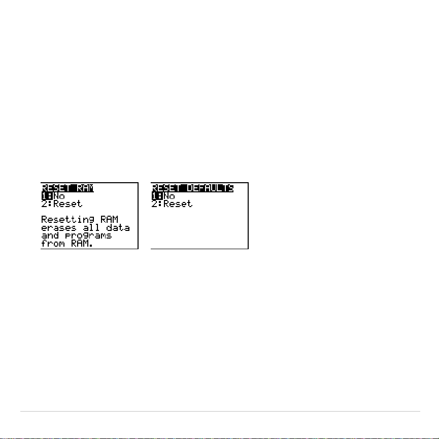
TI-83 Plus Memory and Variable Management 605
and programs in RAM. Resetting RAM or resetting defaults does not
affect variables and applications in user data archive.
Tip:
Before you reset all RAM memory, consider restoring sufficient available
memory by deleting only selected data.
To reset all
RAM
memory or
RAM
defaults on the TI-83 Plus, follow these
steps.
1. From the
RAM ARCHIVE ALL
menu, select
1:ALL RAM
to display the
RESET RAM
menu or
2:Defaults
to display the
RESET DEFAULTS
menu
.
2. If you are resetting RAM, read the message below the
RESET RAM
menu.
•
To cancel the reset and return to the home screen, press
Í
.
•
To erase RAM memory or reset defaults, select
2:Reset
.
Depending on your choice, the message
RAM cleared
or
Defaults
set
is displayed on the home screen.
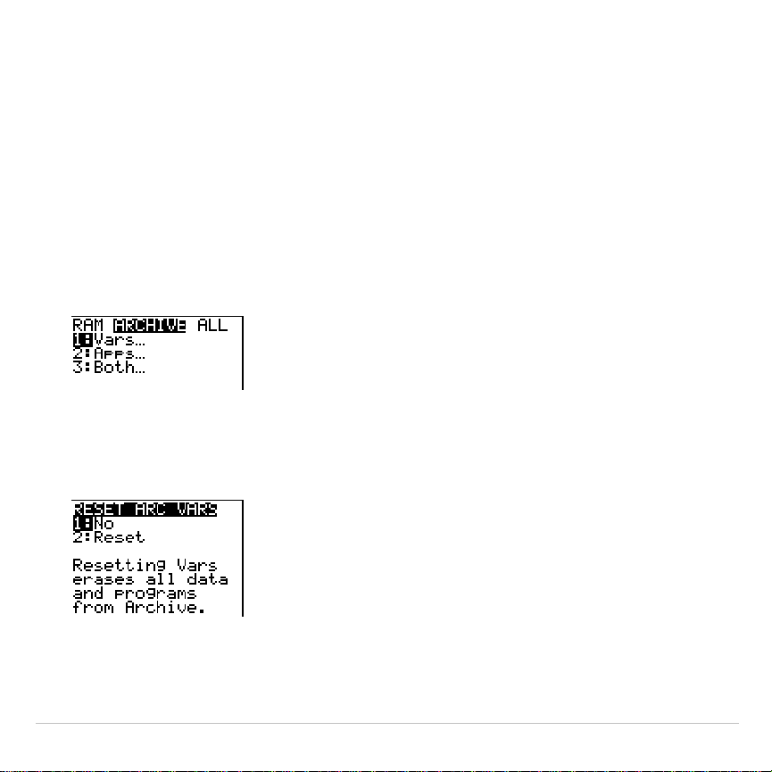
TI-83 Plus Memory and Variable Management 606
Resetting Archive Memory
When resetting archive memory on the TI-83 Plus, you can choose to
delete from user data archive all variables, all applications, or both
variables and applications.
To reset all or part of user data archive memory, follow these steps.
1. From the
RAM ARCHIVE ALL
menu, press
~
to display the
ARCHIVE
menu.
2. Select one of the following:
1:Vars
to display the
RESET ARC VAR
menu
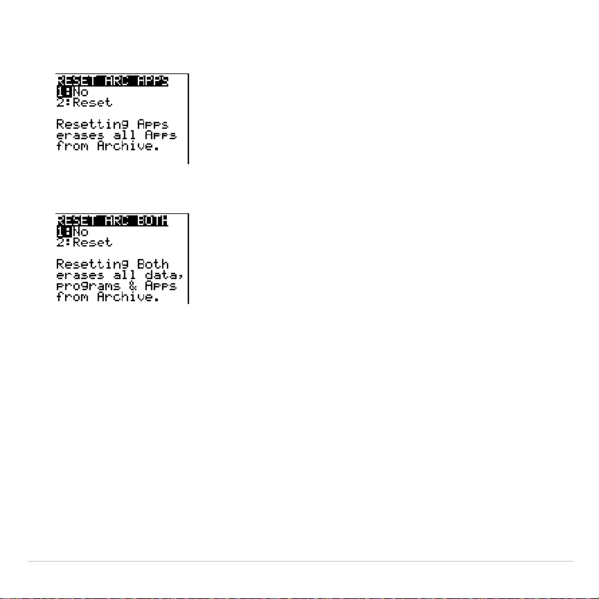
TI-83 Plus Memory and Variable Management 607
2:Apps
to display the
RESET ARC APPS
menu.
3:Both
to display the
RESET ARC BOTH
menu.
3. Read the message below the menu.
•
To cancel the reset and return to the home screen, press
Í
.
•
To continue with the reset, select
2:Reset
. A message indicating
the type of archive memory cleared will be displayed on the home
screen.
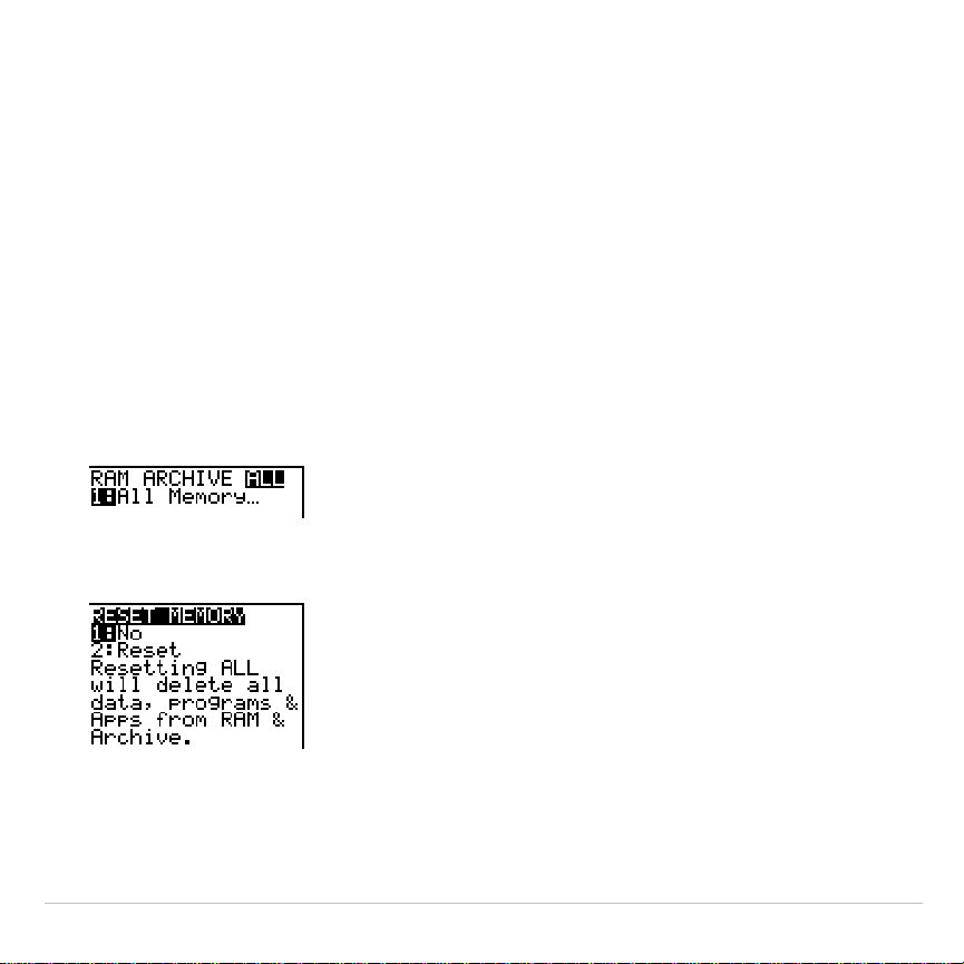
TI-83 Plus Memory and Variable Management 608
Resetting All Memory
When resetting all memory on the TI-83 Plus, RAM and user data
archive memory is restored to factory settings. All nonsystem variables,
applications, and programs are deleted. All system variables are reset to
default settings.
Tip: Before you reset all memory, consider restoring sufficient available
memory by deleting only selected data.
To reset all memory on the TI-83 Plus, follow these steps.
1. From the
RAM ARCHIVE ALL
menu, press
~
~
to display the
ALL
menu.
2. Select
1:All Memory
to display the
RESET MEMORY
menu.

TI-83 Plus Memory and Variable Management 609
3. Read the message below the
RESET MEMORY
menu.
•
To cancel the reset and return to the home screen, press
Í
.
•
To continue with the reset, select
2:Reset
. The message
MEM
cleared
is displayed on the home screen.
Note: When you clear memory, the contrast sometimes changes. If the screen
is faded or blank, adjust the contrast by pressing
y
}
or
†
.

TI-83 Plus Memory and Variable Management 610
Archiving and UnArchiving Variables
Archiving and UnArchiving Variables
Archiving allows you to store data, programs, or other variables to the
user data archive where they cannot be edited or deleted inadvertently.
Archiving also allows you to free up RAM for variables that may require
additional memory.
Archived variables cannot be edited or executed. They can only be seen
and unarchived. For example, if you archive list
L1
, you will see that
L1
exists in memory but if you select it and paste the name
L1
to the home
screen, you won’t be able to see its contents or edit it.
Note: Not all variables may be archived. Not all archived variables may be
unarchived. For example, system variables including r, t, x, y, and
q
cannot be
archived. Apps and Groups always exist in Flash ROM so there is no need to
archive them. Groups cannot be unarchived. However, you can ungroup or
delete them.

TI-83 Plus Memory and Variable Management 611
Variable Type Names
Archive?
(yes/no)
UnArchive?
(yes/no)
Real numbers
A
,
B
, ... ,
Z
yes yes
Complex numbers
A
,
B
, ... ,
Z
yes yes
Matrices
ã
A
ä
,
ã
B
ä
,
ã
C
ä
, ... ,
ã
J
ä
yes yes
Lists
L1
,
L2
,
L3
,
L4
,
L5
,
L6
,
and user-defined
names
yes yes
Programs yes yes
Functions
Y1
,
Y2
, . . . ,
Y9
,
Y0
no not
applicable
Parametric equations
X1T
and
Y1T
, ... ,
X6T
and
Y6T
no not
applicable
Polar functions
r1
,
r2
,
r3
,
r4
,
r5
,
r6
no not
applicable
Sequence functions
u
,
v
,
w
no not
applicable
Stat plots
Plot1, Plot2, Plot3
no not
applicable
Graph databases
GDB1, GDB2,...
yes yes
Graph pictures
Pic1
,
Pic2
, ... ,
Pic9
,
Pic0
yes yes
Strings
Str1
,
Str2
, . . .
Str9
,
Str0
yes yes

TI-83 Plus Memory and Variable Management 612
Variable Type Names
Archive?
(yes/no)
UnArchive?
(yes/no)
Tables
TblStart
,
Tb1
,
TblInput
no not
applicable
Apps
Applications
see Note
above
no
AppVars
Application variables
yes yes
Groups see Note
above
no
Variables with reserved
names
minX
,
maxX
,
RegEQ,
and others
no not
applicable
System variables
Xmin
,
Xmax
, and
others
no not
applicable
Archiving and unarchiving can be done in two ways:
•
Use the
5:Archive
or
6:UnArchive
commands from the
MEMORY
menu
or
CATALOG.
•
Use a Memory Management editor screen.
Before archiving or unarchiving variables, particularly those with a large
byte size (such as large programs) use the
MEMORY
menu to:
•
Find the size of the variable.
•
See if there is enough free space.
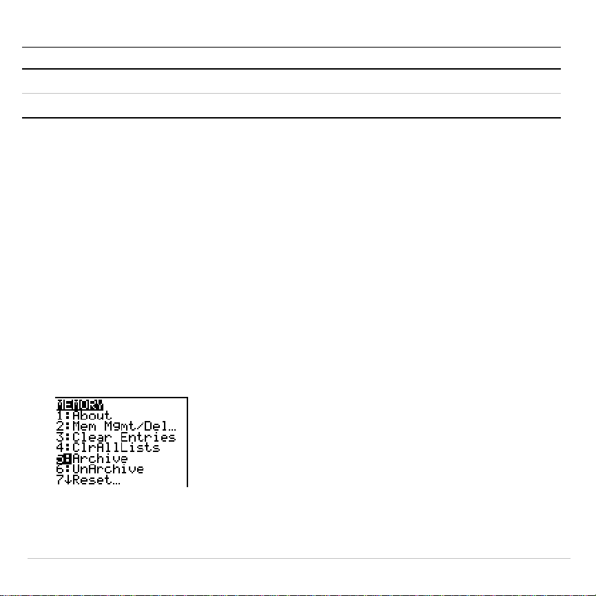
TI-83 Plus Memory and Variable Management 613
For: Sizes must be such that:
Archive Archive free size > variable size
UnArchive RAM free size > variable size
Note:
If there is not enough space, unarchive or delete variables as necessary.
Be aware that when you unarchive a variable, not all the memory associated
with that variable in user data archive will be released since the system keeps
track of where the variable has been and where it is now in RAM.
Even if there appears to be enough free space, you may see a Garbage
Collection message when you attempt to archive a variable. Depending
on the usability of empty blocks in the user data archive, you may need
to unarchive existing variables to create more free space.
To archive or unarchive a list variable (L1) using the Archive/UnArchive
options from the MEMORY menu:
1. Press
y
L
to display the
MEMORY
menu.
2. Select
5:Archive
or
6:UnArchive
to place the command in the edit
screen.
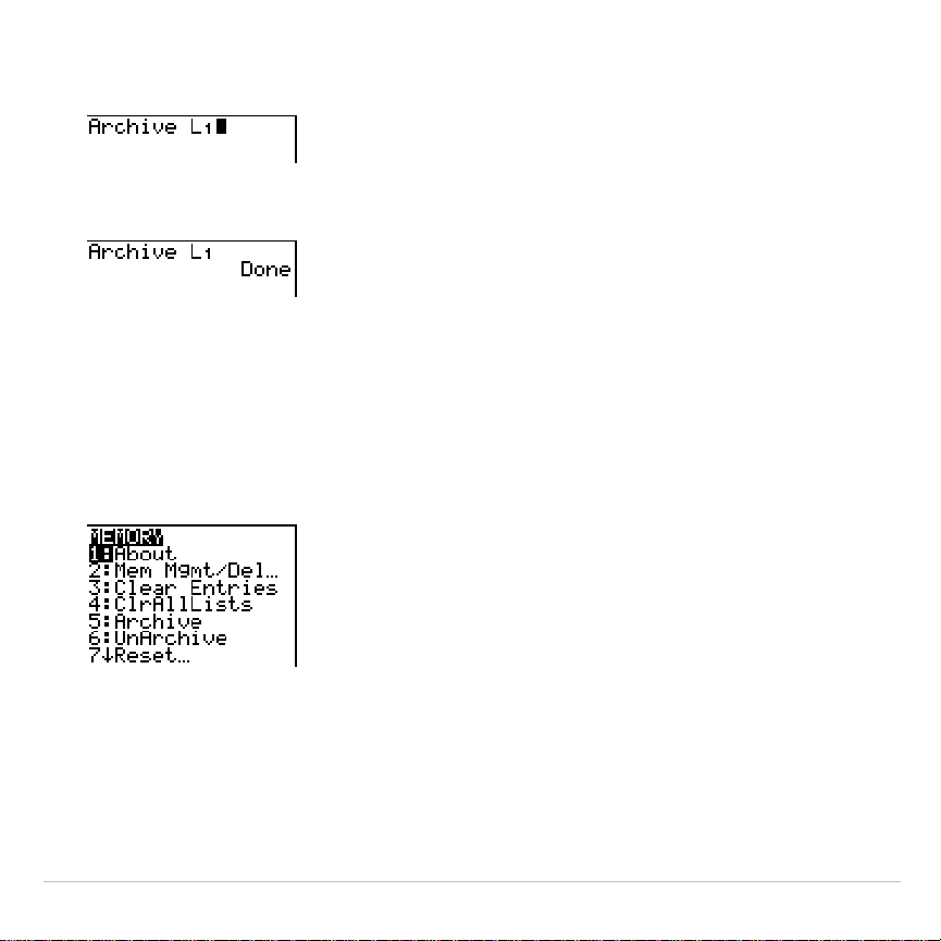
TI-83 Plus Memory and Variable Management 614
3. Press
y
d
to place the
L1
variable in the edit screen.
4. Press
Í
to complete the archive process.
Note: An asterisk will be displayed to the left of the Archived variable name to
indicate it is archived.
To archive or unarchive a list variable (L1) using a Memory Management
editor:
1. Press
y
L
to display the
MEMORY
menu.
2. Select
2:Mem Mgmt/Del...
to display the
MEMORY MANAGEMENT/DELETE
menu.
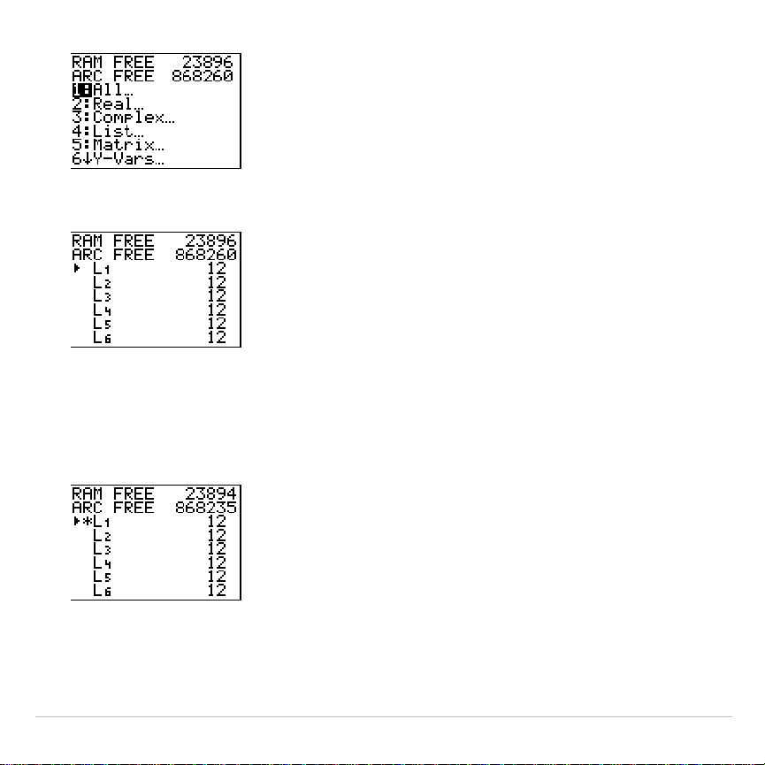
TI-83 Plus Memory and Variable Management 615
3. Select
4:List...
to display the
LIST
menu.
4. Press
Í
to archive
L1
. An asterisk will appear to the left of
L1
to
indicate it is an archived variable. To unarchive a variable in this
screen, put the cursor next to the archived variable and press
Í
.
The asterisk will disappear.
5. Press
y
5
to leave the
LIST
menu.
Note: You can access an archived variable for the purpose of linking, deleting,
or unarchiving it, but you cannot edit it.
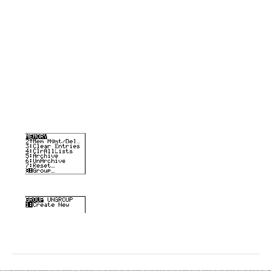
TI-83 Plus Memory and Variable Management 616
Grouping and Ungrouping Variables
Grouping Variables
Grouping allows you to make a copy of two or more variables residing in
RAM and then store them as a group in user data archive. The variables
in RAM are not erased. The variables must exist in RAM before they can
be grouped. In other words, archived data cannot be included in a group.
To create a group of variables:
1. Press
y
L
to display the
MEMORY
menu.
2. Select
8:Group...
to display
GROUP UNGROUP
menu.
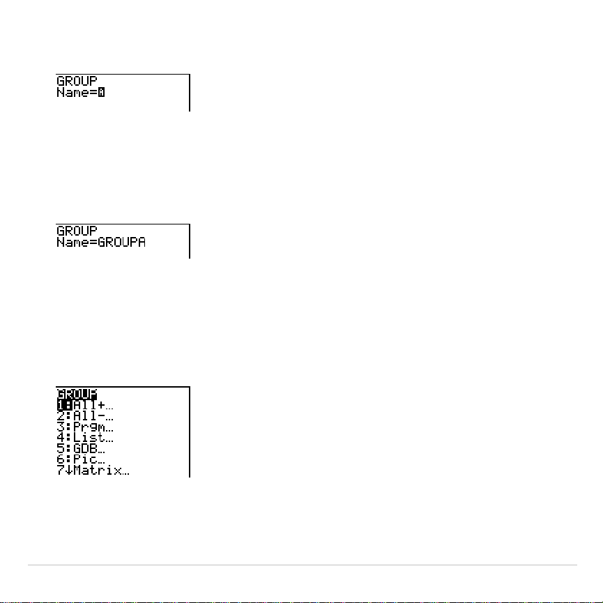
TI-83 Plus Memory and Variable Management 617
3. Press
Í
to display the
GROUP
menu.
4. Enter a name for the new group and press
Í
.
Note: A group name can be one to eight characters long. The first character
must be a letter from A to Z or
q
. The second through eighth characters can
be letters, numbers, or
q
.
5. Select the type of data you want to group. You can select
1:All+
which
shows all variables of all types available and selected. You can also
select
1:All-
which shows all variables of all types available but not
selected. A screen is displayed listing each variable of the type you
selected.
For example, suppose some variables have been created in RAM,
and selecting
1:All-
displays the following screen.
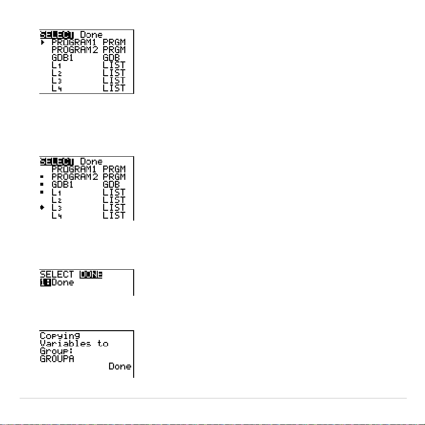
TI-83 Plus Memory and Variable Management 618
6. Press
}
and
†
to move the selection cursor (
4
) next to the first item
you want to copy into a group, and then press
Í
. A small square
will remain to the left of all variables selected for grouping.
Repeat the selection process until all variables for the new group are
selected and then press
~
to display the
DONE
menu.
7. Press
Í
to complete the grouping process.

TI-83 Plus Memory and Variable Management 619
Note:
You can only group variables in RAM. You cannot group some system
variables, such as the last-answer variable
Ans
and the statistical variable
RegEQ
.
Ungrouping Variables
Ungrouping
allows you to make a copy of variables in a group stored in
user data archive and place them ungrouped in
RAM
.
DuplicateName Menu
During the ungrouping action, if a duplicate variable name is detected in
RAM
, the
DUPLICATE NAME
menu is displayed.
DuplicateName
1:Rename
Prompts to rename receiving variable.
2:Overwrite
Overwrites data in receiving duplicate variable.
3:Overwrite All
Overwrites data in all receiving duplicate variables.
4:Omit
Skips transmission of sending variable.
5:Quit
Stops transmission at duplicate variable.
Notes about Menu Items:
•
When you select
1:Rename
, the
Name=
prompt is displayed, and
alpha-lock is on. Enter a new variable name, and then press
Í
.
Ungrouping resumes.
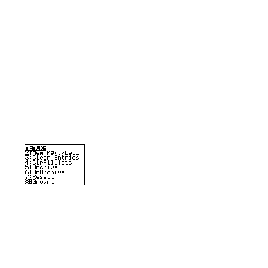
TI-83 Plus Memory and Variable Management 620
•
When you select
2:Overwrite
, the unit overwrites the data of the
duplicate variable name found in RAM. Ungrouping resumes.
•
When you select
3: Overwrite All
, the unit overwrites the data of all
duplicate variable names found in RAM. Ungrouping resumes.
•
When you select
4:Omit
, the unit does not ungroup the variable in
conflict with the duplicated variable name found in RAM. Ungrouping
resumes with the next item.
•
When you select
5:Quit
, ungrouping stops, and no further changes
are made.
To ungroup a group of variables:
1. Press
y
L
to display the
MEMORY
menu.
2. Select
8:Group...
to display the
GROUP UNGROUP
menu.
3. Press
~
to display the
UNGROUP
menu.
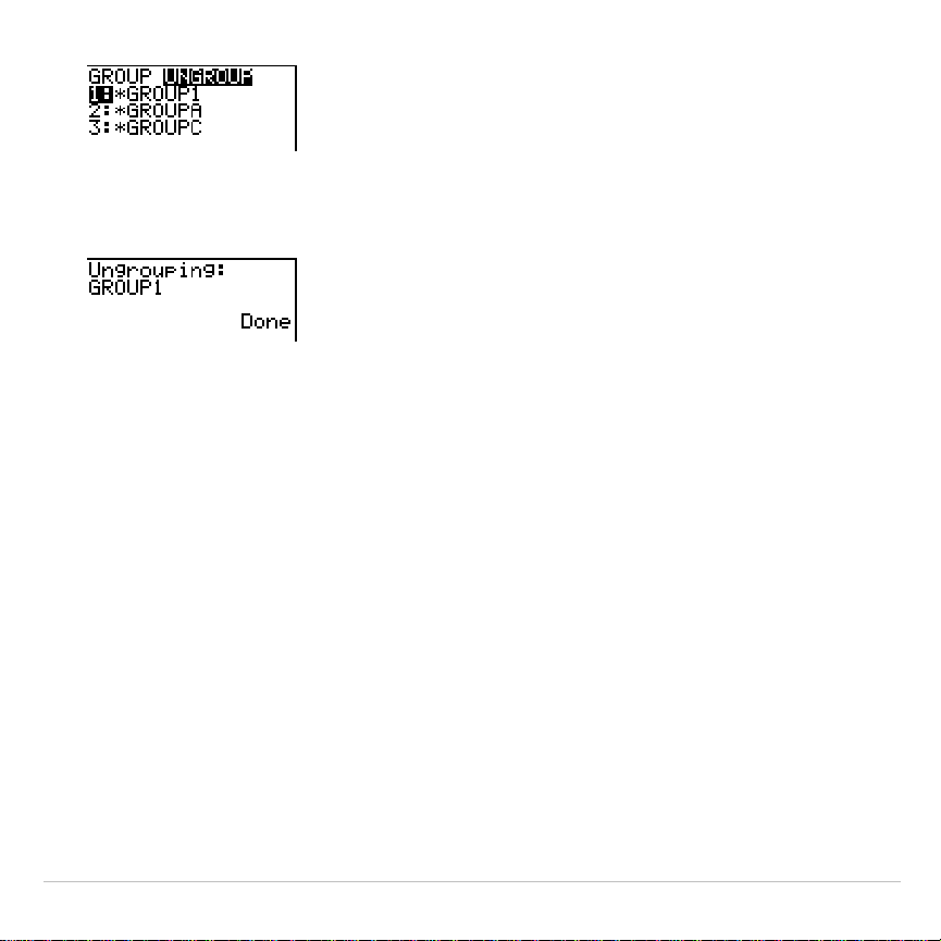
TI-83 Plus Memory and Variable Management 621
4. Press
}
and
†
to move the selection cursor (
4
) next to the group
variable you want to ungroup, and then press
Í
.
The ungroup action is completed.
Note:
Ungrouping does not remove the group from user data archive. You must
delete the group in user data archive to remove it.
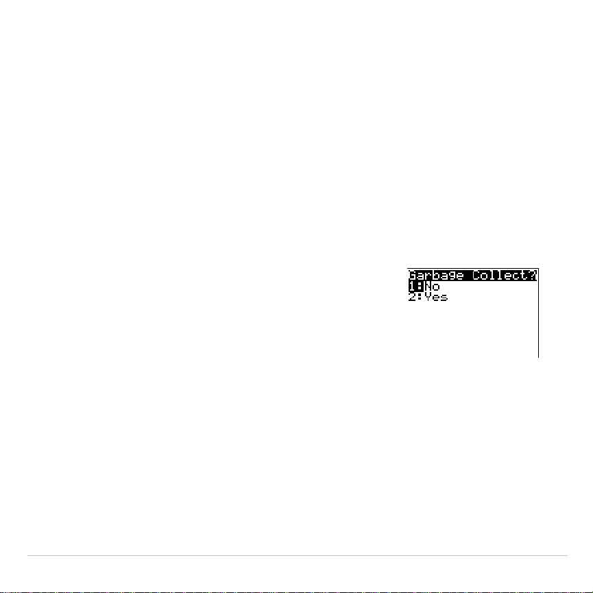
TI-83 Plus Memory and Variable Management 622
Garbage Collection
Garbage Collection Message
If you use the user data archive extensively, you may see a
Garbage
Collect?
message. This occurs if you try to archive a variable when there
is not enough free contiguous archive memory. The TI-83 Plus will
attempt to rearrange the archived variables to make additional room.
Responding to the Garbage Collection Message
•
To cancel, select
1:No
.
•
If you choose
1:No
, the message
ERR:ARCHIVE FULL
will be displayed.
•
To continue archiving, select
2:Yes
.
If you select
2:Yes
, the process message
Garbage Collecting...
or
Defragmenting...
will be displayed.
Note: The process message Defragmenting... is displayed whenever an
application marked for deletion is encountered.
Garbage collection may take up to 20 minutes, depending on how much of
archive memory has been used to store variables.

TI-83 Plus Memory and Variable Management 623
After garbage collection, depending on how much additional space is
freed, the variable may or may not be archived. If not, you can unarchive
some variables and try again.
Why Not Perform Garbage Collection Automatically Without a
Message?
The message:
•
Lets you know an archive will take longer than usual. It also alerts
you that the archive will fail if there is not enough memory.
•
Can alert you when a program is caught in a loop that repetitively fills
the user data archive. Cancel the archive and determine the reason.
Why Is Garbage Collection Necessary?
The user data archive is divided into sectors. When you first begin
archiving, variables are stored consecutively in sector 1. This continues
to the end of the sector.
An archived variable is stored in a continuous block within a single
sector. Unlike an application stored in user data archive, an archived
variable cannot cross a sector boundary. If there is not enough space left
in the sector, the next variable is stored at the beginning of the next
sector. Typically, this leaves an empty block at the end of the previous
sector.
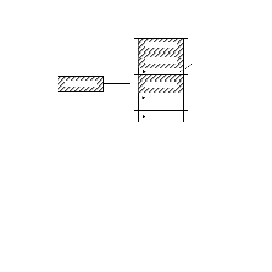
TI-83 Plus Memory and Variable Management 624
Each variable that you archive is stored in the first empty block large
enough to hold it.
This process continues to the end of the last sector. Depending on the
size of individual variables, the empty blocks may account for a
significant amount of space. Garbage collection occurs when the
variable you are archiving is larger than any empty block.
Sector 1
Sector 2
Sector 3
v
a
ri
ab
l
e
A
v
a
ri
ab
l
e
B
v
a
ri
ab
l
e
C
Empty
block
v
a
ri
ab
l
e
D
Depending on its size,
variable D is stored in
one of these locations.
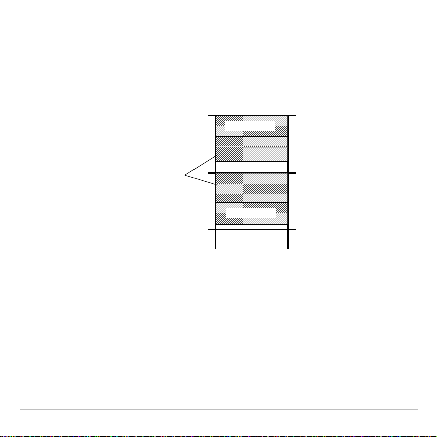
TI-83 Plus Memory and Variable Management 625
How Unarchiving a Variable Affects the Process
When you unarchive a variable, it is copied to RAM but it is not actually
deleted from user data archive memory.
Unarchived variables are “marked for deletion,” meaning they will be
deleted during the next garbage collection.
Sector 1
Sector 2
Sector 3
v
a
ri
ab
l
e
A
v
a
ri
ab
l
e
D
After you unarchive
variables B and C, they
continue to take up
s
p
ace.
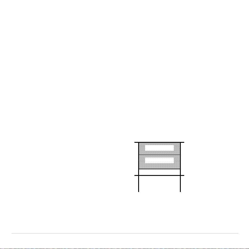
TI-83 Plus Memory and Variable Management 626
If the
MEMORY
Screen Shows Enough Free Space
Even if the
MEMORY
screen shows enough free space to archive a
variable or store an application, you may still get a
Garbage Collect?
message or an
ERR: ARCHIVE FULL
message.
When you unarchive a variable, the
Archive free
amount increases
immediately, but the space is not actually available until after the next
garbage collection.
If the
Archive free
amount shows enough available space for your
variable, there probably will be enough space to archive it after garbage
collection (depending on the usability of any empty blocks).
The Garbage Collection Process
The garbage collection process:
•
Deletes unarchived variables from
the user data archive.
•
Rearranges the remaining
variables into consecutive blocks.
Note: Power loss during garbage collection may cause all memory (RAM and
Archive) to be deleted.
Sector 1
Sector 2
v
a
ri
ab
l
e
A
v
a
ri
ab
l
e
D
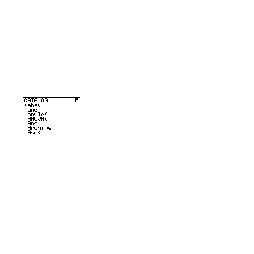
TI-83 Plus Memory and Variable Management 627
Using the GarbageCollect Command
You can reduce the number of automatic garbage collections by
periodically optimizing memory. This is done by using the
GarbageCollect
command.
To use the
GarbageCollect
command, follow these steps.
1. Press
y
ã
CATALOGä
to display the
CATALOG
.
2. Press
†
or
}
to scroll the
CATALOG
until the selection cursor points to
the
GarbageCollect
command.
3. Press
Í
to paste the command to the current screen.
4. Press
Í
to display the
Garbage Collect?
message.
5. Select
2:Yes
to begin garbage collection.
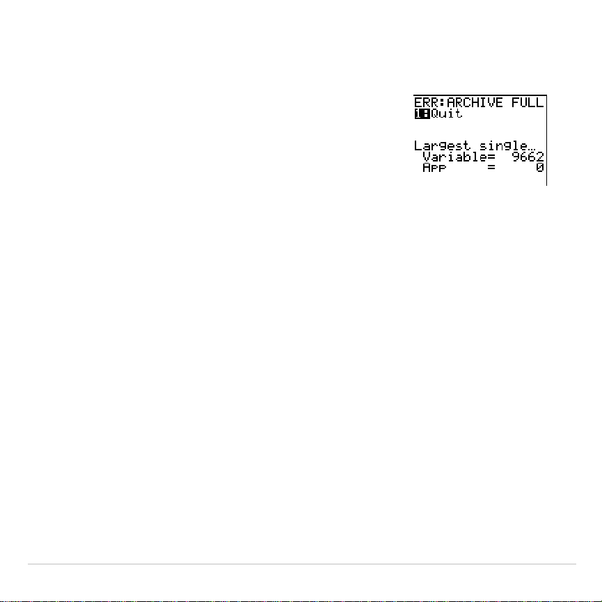
TI-83 Plus Memory and Variable Management 628
ERR:ARCHIVE FULL Message
Even if the
MEMORY
screen shows enough free
space to archive a variable or store an
application, you may still get an
ERR: ARCHIVE
FULL
message.
An
ERR:ARCHIVE FULL
message may be displayed:
•
When there is insufficient space to archive a variable within a
continuous block and within a single sector.
•
When there is insufficient space to store an application within a
continuous block of memory.
When the message is displayed, it will indicate the largest single space
of memory available for storing a variable and an application.
To resolve the problem, use the
GarbageCollect
command to optimize
memory. If memory is still insufficient, you must delete variables or
applications to increase space.
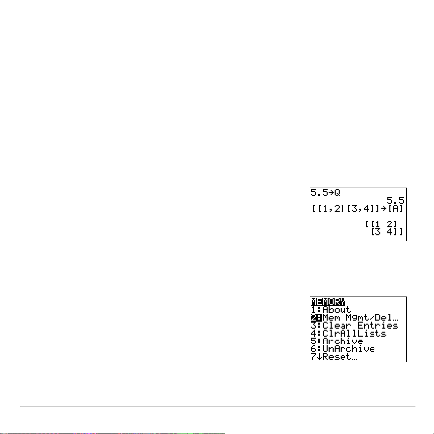
TI-83 Plus Communication Link 629
Chapter 19:
Communication Link
Getting Started: Sending Variables
Getting Started is a fast-paced introduction. Read the chapter for details.
Create and store a variable and a matrix, and then transfer them to another
TI-83 Plus.
1. On the home screen of the sending unit, press
5
Ë
5
¿
ƒ
Q
. Press
Í
to store 5.5
to
Q
.
2. Press
y
H
y
H
1
¢
2
y
I
y
H
3
¢
4
y
I
y
I
¿
y
>
1
. Press
Í
to store the matrix to
[A]
.
3. On the sending unit, press
y
L
to display
the
MEMORY
menu.
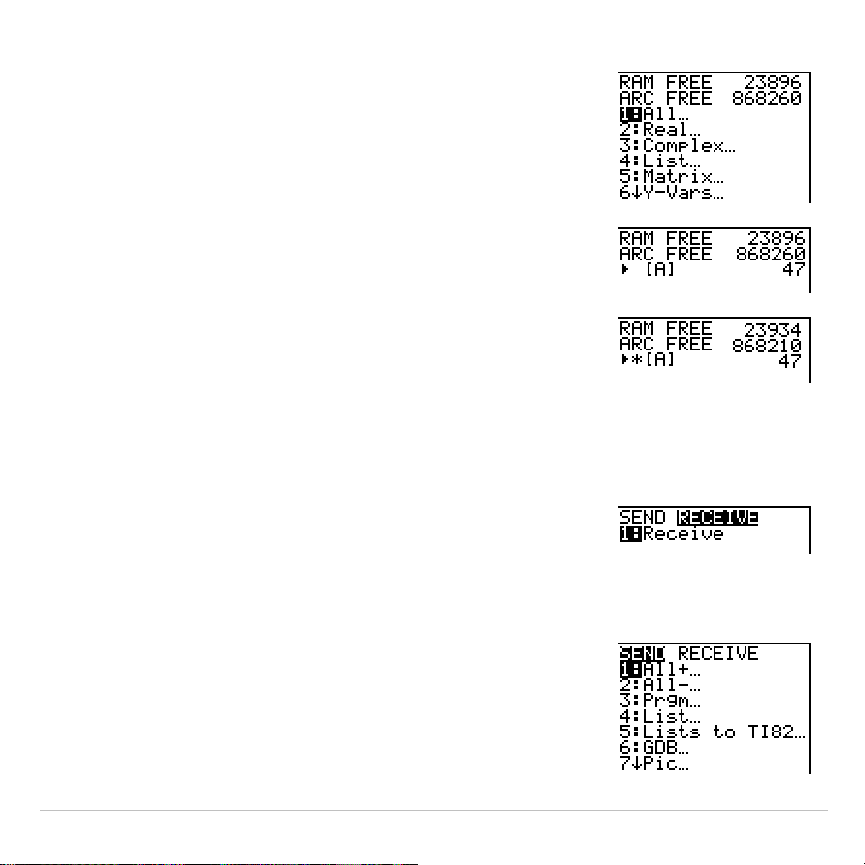
TI-83 Plus Communication Link 630
4. On the sending unit, press
2
to select
2:Mem
Mgmt/Del
. The
MEMORY MANAGEMENT
menu is
displayed.
5. On the sending unit, press
5
to select
5:Matrix
.
The
MATRIX
editor screen is displayed.
6. On the sending unit, press
Í
to archive
[A]
.
An asterisk (
*
) will appear, signifying that
[A]
is
now archived.
7. Connect the calculators with the link cable.
Push both ends in firmly.
8. On the receiving unit, press
y
8
~
to
display the
RECEIVE
menu. Press
1
to select
1:Receive
. The message
Waiting
...
is displayed
and the busy indicator is on.
9. On the sending unit, press
y
8
to display
the
SEND
menu.
10.Press
2
to select
2:All
N
. The
All
N
SELECT
screen
is displayed.
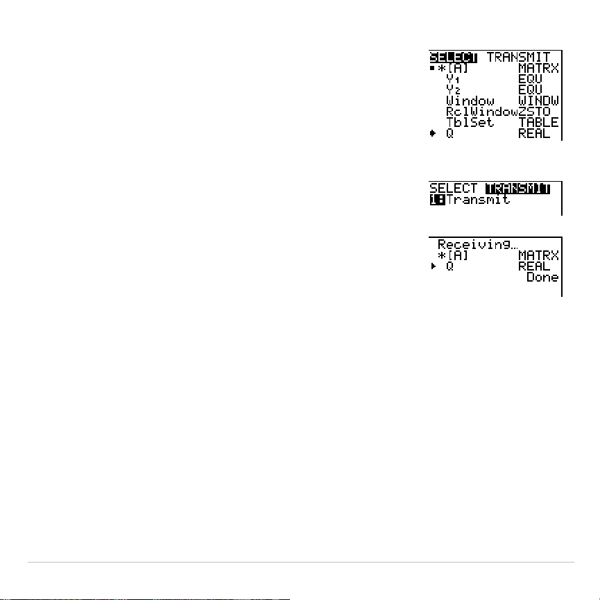
TI-83 Plus Communication Link 631
11.Press
†
until the selection cursor (
4
) is next to
[A] MATRX
. Press
Í
.
12.Press
†
until the selection cursor is next to
Q REAL
. Press
Í
. A square dot next to
[A]
and
Q
indicates that each is selected to send.
13.On the sending unit, press
~
to display the
TRANSMIT
menu.
14.On the sending unit, press
1
to select
1:Transmit
and begin transmission. The receiving unit
displays the message
Receiving...
.When the
items are transmitted, both units display the
name and type of each transmitted variable.

TI-83 Plus Communication Link 632
TI-83 Plus Silver Edition LINK
This chapter describes how to communicate with compatible TI units. A
unit-to-unit link cable is included with the TI-83 Plus Silver Edition for this
purpose.
The TI-83 Plus Silver Edition has a port to connect and communicate
with:
•
Another TI-83 Plus Silver Edition
•
A TI-83 Plus
•
A TI-83
•
A TI-82
•
A TI-73
•
A CBL 2/CBL, or a CBR
With the
TI™ Connect
or
TI-GRAPH LINK™
software and a
TI-GRAPH LINK
cable, you can link the TI-83 Plus Silver Edition to a personal computer.

TI-83 Plus Communication Link 633
Connecting Two Calculators with a Unit-to-Unit Cable
The TI-83 Plus link port is located at the center of the bottom edge of the
calculator.
1. Firmly insert either end of the unit-to-unit cable into the port.
2. Insert the other end of the cable into the other calculator’s port.
Linking to the CBL/CBR System
The CBL 2/CBL and the CBR are optional accessories that also connect
to a TI-83 Plus with the unit-to-unit link cable. With a CBL 2/CBL or CBR
and a TI-83 Plus, you can collect and analyze real-world data. The
software that enables this communication is built into the TI-83 Plus.
(Chapter 14).
Linking to a Computer
TI-GRAPH LINK™
is an accessory that links a TI-83 Plus to enable
communication with a computer. A Macintosh
ë
-compatible
TI-GRAPH LINK
is available separately.
You can access
TI-GRAPH LINK
guidebooks through
education.ti.com/guides
.

TI-83 Plus Communication Link 634
Selecting Items to Send
LINK SEND Menu
To display the
LINK SEND
menu, press
y
8
.
SEND RECEIVE
1:All+
...
Displays all items as selected, including RAM and Flash
applications.
2:All
N
...
Displays all items as deselected.
3:Prgm
...
Displays all program names.
4:List
...
Displays all list names.
5:Lists to TI82
...
Displays list names
L1
through
L6
.
6:GDB
...
Displays all graph databases.
7:Pic
...
Displays all picture data types.
8:Matrix
...
Displays all matrix data types.
9:Real
...
Displays all real variables.
0:Complex
...
Displays all complex variables.
A:Y-Vars
...
Displays all
Y=
variables.
B:String
...
Displays all string variables.
C:Apps
...
Displays all software applications.
D:AppVars
...
Displays all software application variables.
E:Group
...
Displays all grouped variables.
F:SendId
Sends the Calculator ID number immediately. (You do not
need to select
SEND
.)

TI-83 Plus Communication Link 635
SEND RECEIVE
G:SendOS
Sends operating system updates to another
TI-83 Plus Silver Edition or TI-83 Plus.
H:Back Up
...
Selects all RAM and mode settings (no Flash applications
or archived items) for backup to another
TI-83 Plus Silver Edition or to a TI-83 Plus.
When you select an item on the
LINK SEND
menu, the corresponding
SELECT
screen is displayed.
Note: Each
SELECT
screen, except
All+…
, is initially displayed with nothing pre-
selected.
All+…
is displayed with everything pre-selected.
To select items to send:
1. Press
y
8
on the sending unit to display the
LINK SEND
menu.
2. Select the menu item that describes the data type to send. The
corresponding
SELECT
screen is displayed.
3. Press
}
and
†
to move the selection cursor (
4
) to an item you want
to select or deselect.
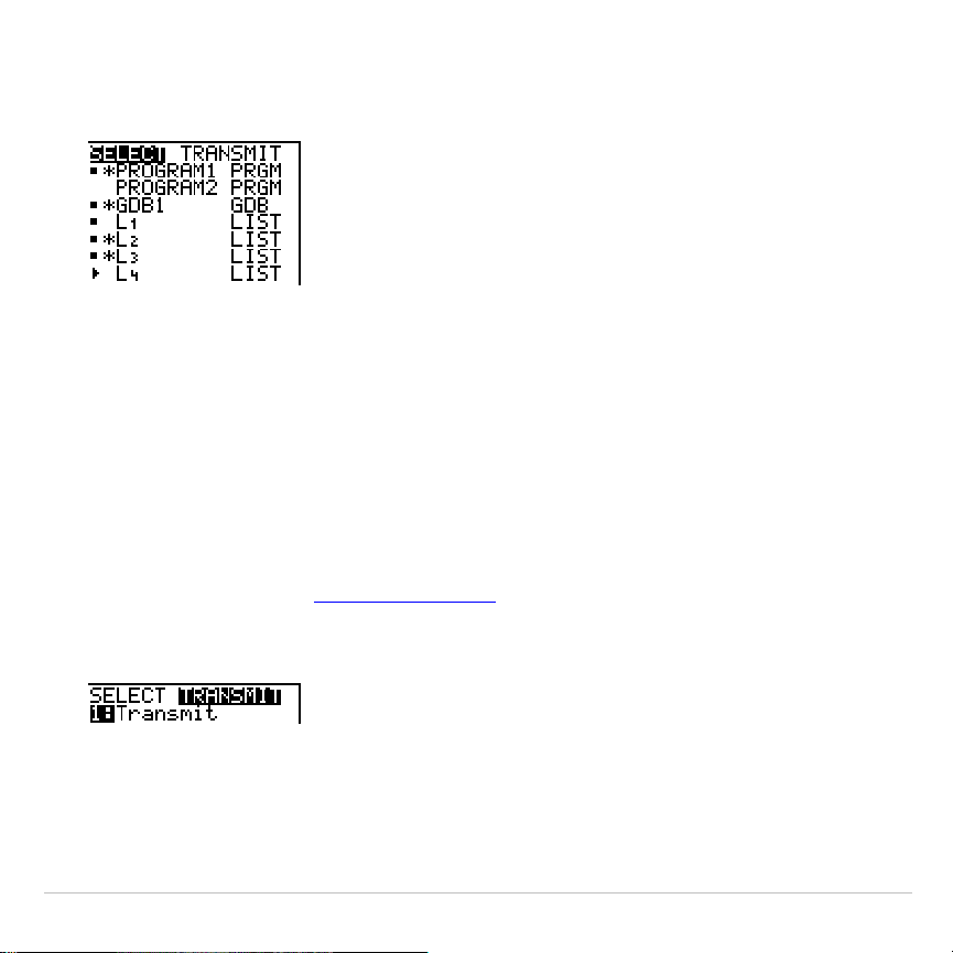
TI-83 Plus Communication Link 636
4. Press
Í
to select or deselect the item. Selected names are
marked with a
0
.
Note:
An asterisk (
*
) to the left of an item indicates the item is archived
(Chapter 18).
5. Repeat steps 3 and 4 to select or deselect additional items.
Sending the Selected Items
After you have selected items to send on the sending unit and set the
receiving unit to receive, follow these steps to transmit the items. To set
the receiving unit, see
Receiving Items
.
1. Press
~
on the sending unit to display the
TRANSMIT
menu.
2. Confirm that
Waiting...
is displayed on the receiving unit, which
indicates it is set to receive.
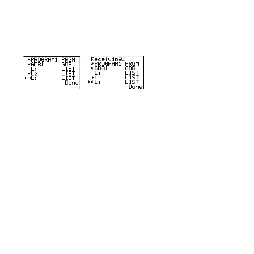
TI-83 Plus Communication Link 637
3. Press
Í
to select
1:Transmit
. The name and type of each item are
displayed line-by-line on the sending unit as the item is queued for
transmission, and then on the receiving unit as each item is
accepted.
Note: Items sent from the RAM of the sending unit are transmitted to the
RAM of the receiving unit. Items sent from user data archive of the sending
unit are transmitted to user data archive of the receiving unit.
After all selected items have been transmitted, the message
Done
is
displayed on both calculators. Press
}
and
†
to scroll through the
names.
Stopping a Transmission
To stop a link transmission, press
É
. The
Error in Xmit
menu is displayed
on both units. To leave the error menu, select
1:Quit
.

TI-83 Plus Communication Link 638
Sending to a TI-83 Plus Silver Edition or TI-83 Plus
You can transfer variables (all types), programs, and Flash applications
to another TI-83 Plus Silver Edition or TI-83 Plus. You can also backup
the RAM memory of one unit to another.
Note: Keep in mind that the TI
.
83 Plus has less Flash memory than the
TI-83 Plus Silver Edition.
•
Variables stored in RAM on the sending TI-83 Plus Silver Edition will
be sent to the RAM of the receiving TI-83 Plus Silver Edition or
TI-83 Plus.
•
Variables and applications stored in the user data archive of the
sending TI-83 Plus Silver Edition will be sent to the user data archive
of the receiving TI-83 Plus Silver Edition or TI-83 Plus.
After sending or receiving data, you can repeat the same transmission to
additional TI-83 Plus Silver Edition or TI-83 Plus units—from either the
sending unit or the receiving unit—without having to reselect data to
send. The current items remain selected. However, you cannot repeat
transmission if you selected
All+
or
All
.
.

TI-83 Plus Communication Link 639
To send data to an additional TI-83 Plus Silver Edition or a TI-83 Plus:
1. Use a unit-to-unit cable to link two units together.
2. On the sending unit press
y
8
and select a data type and items
to
SEND
.
3. Press
~
on the sending unit to display the
TRANSMIT
menu.
4. On the other unit, press
y
8
~
to display the
RECEIVE
menu.
5. Press
Í
on the receiving unit.
6. Press
Í
on the sending unit. A copy of the selected item(s) is
sent to the receiving unit.
7. Disconnect the link cable only from the receiving unit and connect it
to another unit.
8. Press
y
8
on the sending unit.
9. Select only the data type. For example, if the unit just sent a list,
select
4:LIST
.
Note: The item(s) you want to send are pre-selected from the last
transmission. Do not select or deselect any items. If you select or deselect

TI-83 Plus Communication Link 640
an item, all selections or deselections from the last transmission are
cleared.
10.Press
~
on the sending unit to display the
TRANSMIT
menu.
11.On the new receiving unit, press
y
8
~
to display the
RECEIVE
menu.
12.Press
Í
on the receiving unit.
13.Press
Í
on the sending unit. A copy of the selected item(s) is
sent to the receiving unit.
14.Repeat steps 7 through 13 until the items are sent to all additional
units.
Sending to a TI-83
You can send all variables from a TI-83 Plus to a TI-83
except
Flash
applications, application variables, grouped variables, new variable
types, or programs with new features in them (such as
Archive
,
UnArchive
,
Asm(
,
AsmComp
, and
AsmPrgm
)
.
If archived variables on the TI-83 Plus are variable types recognized and
used on the TI-83, you can send these variables to the TI-83. They will
be automatically sent to the RAM of the TI-83 during the transfer
process.

TI-83 Plus Communication Link 641
Note:
You cannot perform a RAM memory backup from a TI-83 Plus to a TI-83
or from a TI-83 to a TI-83 Plus.
To send data to a TI-83:
1. Use a unit-to-unit cable to link the two units together.
2. Set the TI-83 to receive.
3. Press
y
8
on the sending TI-83 Plus to display the
LINK SEND
menu.
4. Select the menu of the items you want to transmit.
5. Press
~
on the sending TI-83 Plus to display the
LINK TRANSMIT
menu.
6. Confirm that the receiving unit is set to receive.
7. Press
Í
on the sending TI-83 Plus to select
1:Transmit
and begin
transmitting.
Sending Lists to a TI-82
The only data type you can transmit from a TI-83 Plus to a TI-82 is real
list data stored in
L
1
through
L
6
(with up to 99 elements for each list). If
dimension is greater than 99 for a TI-83 Plus list that is selected to be
sent, the receiving TI-82 will truncate the list at the ninety-ninth element
during transmission.

TI-83 Plus Communication Link 642
Note:
You cannot perform a memory backup from a TI-83 Plus to a TI-82 or
from a TI-82 to a TI-83 Plus.
To send lists to a TI-82:
1. Use a unit-to-unit cable to link the two units together.
2. Set the TI-82 to receive.
3. Press
y
8
5
on the sending TI-83 Plus to select
5:Lists to TI82
.
The
SELECT
screen is displayed.
4. Select each list to transmit.
5. Press
~
to display the
LINK TRANSMIT
menu.
6. Confirm that the receiving unit is set to receive.
7. Press
Í
to select
1:Transmit
and begin transmitting.
Sending to a TI-73
You can send real numbers, pics, real lists
L
1
through
L
6
, and named
lists from a TI-73 to a TI-83 Plus or from a TI-83 Plus to a TI-73.
Since the Theta symbol (
q
) is not recognized by the TI-73, you cannot
include this symbol in any list names sent to the TI-73.

TI-83 Plus Communication Link 643
Note:
You cannot perform a RAM memory backup from a TI-83 Plus to a TI-73
or from a to a TI-73 to a TI-83 Plus.
To transmit data to a TI-73:
1. Use a unit-to-unit cable to link two units together.
2. Set the TI-73 to receive.
3. Press
y
8
2
on the sending TI-83 Plus to select
2:All-...
. The
SELECT
screen is displayed.
4. Select items you want to send.
5. Press
~
on the sending TI-83 Plus to display the
LINK TRANSMIT
menu.
6. Confirm that the receiving unit is set to receive.
7. Press
Í
on the sending TI-83 Plus to select
1:Transmit
and begin
transmitting.
TI-83 Plus Communication Link 644
Receiving Items
LINK RECEIVE Menu
To display the
LINK RECEIVE
menu, press
y
8
~
.
SEND RECEIVE
1:Receive
Sets unit to receive data transmission.
Receiving Unit
When you select
1:Receive
from the
LINK RECEIVE
menu on the receiving
unit, the message
Waiting...
and the busy indicator are displayed. The
receiving unit is ready to receive transmitted items. To exit the receive
mode without receiving items, press
É
, and then select
1:Quit
from the
Error in Xmit
menu.
When transmission is complete, the unit exits the receive mode. You can
select
1:Receive
again to receive more items. The receiving unit then
displays a list of items received. Press
y
5
to exit the receive mode.
DuplicateName Menu
During transmission, if a variable name is duplicated, the
DuplicateName
menu is displayed on the receiving unit.
TI-83 Plus Communication Link 645
DuplicateName
1:Rename
Prompts to rename receiving variable.
2:Overwrite
Overwrites data in receiving variable.
3:Omit
Skips transmission of sending variable.
4:Quit
Stops transmission at duplicate variable.
When you select
1:Rename
, the
Name=
prompt is displayed, and alpha-
lock is on. Enter a new variable name, and then press
Í
.
Transmission resumes.
When you select
2:Overwrite
, the sending unit’s data overwrites the
existing data stored on the receiving unit. Transmission resumes.
When you select
3:Omit
, the sending unit does not send the data in the
duplicated variable name. Transmission resumes with the next item.
When you select
4:Quit
, transmission stops, and the receiving unit exits
receive mode.
Receiving from a TI-83 Plus Silver Edition or TI-83 Plus
The TI-83 Plus Silver Edition and the TI-83 Plus are totally compatible.
Keep in mind, however, that the TI-83 Plus has less Flash memory than
a TI-83 Plus Silver Edition.

TI-83 Plus Communication Link 646
Receiving from a TI-83
You can transfer all variables and programs from a TI-83 to a TI-83 Plus
if
they fit in the RAM of the TI-83 Plus. The RAM of the TI-83 Plus is
slightly less than the RAM of the TI-83.
Receiving from a TI-82 — Resolved Differences
Generally, you can transmit items to a TI-83 Plus from a TI-82, but
differences between the two products may affect some transmitted data.
This table shows differences for which the software built into the
TI-83 Plus automatically adjusts when a TI-83 Plus receives TI-82 data.
TI
.
82 TI-83 Plus
n
Min PlotStart
n
Start
n
Min
U
n
u
V
n
v
U
n
Start u(
n
Min)
V
n
Start v(
n
Min)
TblMin TblStart
For example, if you transmit a program that contains
n
Start
on a
command line from a TI-82 to a TI-83 Plus, you will see that
n
Min
has
automatically replaced
n
Start
on the command line of the TI-83 Plus.

TI-83 Plus Communication Link 647
Note:
You can transfer all real variables, pics, and programs from a TI-82 to a
TI-83 Plus
if
they fit in the RAM of the TI-83 Plus. The RAM of the TI-83 Plus is
slightly less than the RAM of the TI-82.
Receiving from a TI-82 — Unresolved Differences
The software built into the TI-83 Plus cannot resolve some differences
between the TI-82 and TI-83 Plus. These differences are described
below.
You must edit the transmitted data on the receiving TI-83 Plus to account
for these differences. If you do not edit these differences, the TI-83 Plus
will misinterpret the data.
•
The TI-83 Plus reinterprets TI-82 prefix functions to include open
parentheses, which may add extraneous parentheses to transmitted
expressions.
For example, if you transmit
sin X+5
from a TI-82 to a TI-83 Plus, the
TI-83 Plus reinterprets it as
sin(X+5
. Without a closing parenthesis
after
X
, the TI-83 Plus interprets this as
sin(X+5)
, not the sum of
5
and
sin(X)
.
•
If a TI-82 transmits an instruction that the TI-83 Plus cannot translate,
the
ERR:INVALID
menu displays when the TI-83 Plus attempts to
execute the instruction.

TI-83 Plus Communication Link 648
For example, on the TI-82, the character group
Un-1
is pasted to the
cursor location when you press
y
[
Un
N
1
]. The TI-83 Plus cannot
directly translate
Un-1
to the TI-83 Plus syntax
u(n
N
1)
, so the
ERR:INVALID
menu is displayed.
Note: TI-83 Plus implied multiplication rules differ from those of the TI-82.
For example, the TI-83 Plus evaluates
1
à
2X
as
(1
à
2)
ä
X
, while the TI-82
evaluates
1
à
2X
as
1
à
(2
ä
X)
(Chapter 2).
Receiving from a TI-73
The TI-83 Plus can receive real numbers, pics, real lists
L1
through
L6
,
and named lists from a TI-73.
Categorical lists (lists containing alpha characters as list elements)
cannot be sent from a TI-73 to a TI-83 Plus.
To transmit data to a TI-83 Plus from a TI-73:
1. Set the TI-83 Plus to receive.
2. Press
Œ
on the sending TI-73 to display the
APPLICATIONS
menu.
3. Press
Í
on the sending TI-73 to select
1:Link
and display the
LINK
SEND
menu.
4. Choose
0:Vars to TI83
. and then select the items you want to send.

TI-83 Plus Communication Link 649
5. Press
~
on the sending TI-73 to display the
LINK TRANSMIT
menu.
6. Confirm that the receiving unit is set to receive.
7. Press
Í
on the sending TI-73 to select
1:Transmit
and begin
transmitting.

TI-83 Plus Communication Link 650
Backing Up RAM Memory
Warning:
H:Back Up
overwrites the RAM memory and mode settings in
the receiving unit. All information in the RAM memory of the receiving
unit is lost.
Note: Archived items on the receiving unit are not overwritten.
You can backup the contents of RAM memory and mode settings (no
Flash applications or archived items) to another TI-83 Plus Silver Edition.
You can also backup RAM memory and mode settings to a TI-83 Plus.
To perform a RAM memory backup:
1. Use a unit-to-unit cable to link two TI-83 Plus Silver Edition units, or a
TI-83 Plus Silver Edition and a TI-83 Plus together.
2. On the sending unit press
y
8
and select
H:Back Up
. The
MEMORYBACKUP
screen displays.
3.On the receiving unit, press
y
8
~
to display the RECEIVE
menu.
4.Press
Í
on the receiving unit.
TI-83 Plus Communication Link 651
5.Press
Í
on the sending unit. A
WARNING — Backup
message
displays on the receiving unit.
6.Press
Í
on the receiving unit to continue the backup.
— or —
Press
2:Quit
on the receiving unit to cancel the backup and return to
the
LINK SEND
menu
Note: If a transmission error is returned during a backup, the receiving unit
is reset.
Memory Backup Complete
When the backup is complete, both the sending calculator and receiving
calculator display a confirmation screen.

TI-83 Plus Communication Link 652
Error Conditions
A transmission error occurs after one or two seconds if:
•
A cable is not attached to the sending unit.
•
A cable is not attached to the receiving unit.
Note:
If the cable is attached, push it in firmly and try again.
•
The receiving unit is not set to receive transmission.
•
You attempt a backup between a TI-73, a TI-82, or a TI-83 and a
TI-83 Plus.
•
You attempt a data transfer from a TI-83 Plus to a TI-83, TI-82, or
TI-73 with variables or features not recognized by the TI-83, TI-82, or
TI-73.
•
New variable types and features not recognized by the TI-83, TI-82,
or TI-73 include applications, application variables, grouped
variables, new variable types, or programs with new features in them
such as
Archive
,
UnArchive
,
SendID
,
SendOS
,
Asm(
,
AsmComp(
, and
AsmPrgm
.
•
You attempt a data transfer from a TI-83 Plus to a TI-82 with data
other than real lists
L
1
through
L
6
or without using menu item
5:Lists to TI82
.

TI-83 Plus Communication Link 653
•
You attempt a data transfer from a TI-83 Plus to a TI-73 with data
other than real numbers, pics, real lists
L1
through
L6
or named lists
with
q
as part of the name.
Although a transmission error does not occur, these two conditions may
prevent successful transmission.
•
You try to use
Get(
with a calculator instead of a CBL 2/CBL or CBR.
•
You try to use
GetCalc(
with a TI-83 instead of a
TI-83 Plus Silver Edition or TI-83 Plus.
Insufficient Memory in Receiving Unit
During transmission, if the receiving unit does not have sufficient
memory to receive an item, the
Memory Full
menu is displayed on the
receiving unit.
•
To skip this item for the current transmission, select
1:Omit
.
Transmission resumes with the next item.
•
To cancel the transmission and exit receive mode, select
2:Quit
.

TI-83 Plus Tables and Reference Information 654
Appendix A:
Tables and Reference Information
Table of Functions and Instructions
Functions return a value, list, or matrix. You can use functions in an
expression. Instructions initiate an action. Some functions and instructions
have arguments. Optional arguments and accompanying commas are
enclosed in brackets ( [ ] ). For details about an item, including argument
descriptions and restrictions, turn to the page listed on the right side of the
table.
From the
CATALOG
, you can paste any function or instruction to the home
screen or to a command line in the program editor. However, some
functions and instructions are not valid on the home screen. The items in
this table appear in the same order as they appear in the
CATALOG
.
†
indicates either keystrokes that are valid in the program editor only or
ones that paste certain instructions when you are in the program editor.
Some keystrokes display menus that are available only in the program
editor. Others paste mode, format, or table-set instructions only when you
are in the program editor.

TI-83 Plus Tables and Reference Information 655
Function or Instruction/
Arguments Result
Key or Keys/
Menu or Screen/Item
abs(
value
)
Returns the absolute value of a real
number, expression, list, or matrix.
NUM
1:abs(
abs(
complex value
)
Returns the magnitude of a complex
number or list.
CPX
5:abs(
valueA
and
valueB
Returns 1 if both
valueA
and
valueB
are
ƒ
0
.
valueA
and
valueB
can be
real numbers, expressions, or lists.
y
:
LOGIC
1:and
angle(
value
)
Returns the polar angle of a complex
number or list of complex numbers.
CPX
4:angle(
ANOVA(
list1
,
list2
[
,
list3
,
...
,
list20
]
)
Performs a one-way analysis of
variance for comparing the means of
two to 20 populations.
…
TESTS
F:ANOVA(
Ans
Returns the last answer.
y
Z
Archive
Moves the specified variables from
RAM to the user data archive
memory.
y
L
5:Archive
Asm(
assemblyprgmname
)
Executes an assembly language
program.
y
N
Asm(
AsmComp(
p
r
g
mASM1,
p
rgmASM2
)
Compiles an assembly language
program written in ASCII and stores
the hex version.
y
N
AsmComp(
AsmPrgm
Must be used as the first line of an
assembly language program.
y
N
AsmPrgm

TI-83 Plus Tables and Reference Information 656
Function or Instruction/
Arguments Result
Key or Keys/
Menu or Screen/Item
augment(
matrixA
,
matrixB
)
Returns a matrix, which is
matrixB
appended to
matrixA
as new
columns.
y
>
MATH
7:augment(
augment(
listA
,
listB
)
Returns a list, which is
listB
concatenated to the end of
listA
.
y
9
OPS
9:augment(
AxesOff
Turns off the graph axes. †
y
.
AxesOff
AxesOn
Turns on the graph axes. †
y
.
AxesOn
a+b
i
Sets the mode to rectangular
complex number mode (a+b
i
).
†
z
a+b
i
bal(
npmt
[
,
roundvalue
]
)
Computes the balance at
n
p
mt
for an
amortization schedule using stored
values for
PV
,
æ
, and
PMT
and
rounds the computation to
roundvalue.
Œ
1:Finance
CALC
9:bal(
binomcdf(
numtria
)
Computes a cumulative probability at
x
for the discrete binomial distribution
with the specified
numtrials
and
probability
p
of success on each trial.
y
=
DISTR
A:binomcdf(
binompdf(
numtrials
,
p
[
,
x
]
)
Computes a probability at
x
for the
discrete binomial distribution with the
specified
numtrials
and probability
p
of success on each trial.
y
=
DISTR
0:binompdf(

TI-83 Plus Tables and Reference Information 657
Function or Instruction/
Arguments Result
Key or Keys/
Menu or Screen/Item
c
2
cdf(
lowerbound
,
upperbound
,
df
)
Computes the
c
2
distribution
probability between
lowerbound
and
u
pp
erbound
for the specified degrees
of freedom
df
.
y
=
DISTR
7:
c
2
cdf(
c
2
pdf(
x
,
df
)
Computes the probability density
function (pdf) for the
c
2
distribution at
a specified
x
value for the specified
degrees of freedom
df
.
y
=
DISTR
6:
c
2
pdf(
c
2
.
Test(
observedmatrix
,
ex
p
ectedmatrix
[
,
drawflag
]
)
Performs a chi-square test.
draw
f
la
g
=
1
draws results;
drawflag
=
0
calculates results.
†
…
TESTS
C:
c
2-
Test(
Circle(
X
,
Y
,
radius
)
Draws a circle with center (
X
,
Y
) and
radius
.
y
<
DRAW
9:Circle(
Clear Entries
Clears the contents of the Last Entry
storage area.
y
L
MEMORY
3:Clear Entries
ClrAllLists
Sets to
0
the dimension of all lists in
memory.
y
L
MEMORY
4:ClrAllLists
ClrDraw
Clears all drawn elements from a
graph or drawing.
y
<
DRAW
1:ClrDraw
ClrHome
Clears the home screen. †
I/O
8:ClrHome

TI-83 Plus Tables and Reference Information 658
Function or Instruction/
Arguments Result
Key or Keys/
Menu or Screen/Item
ClrList
listname1
[
,
listname2
, ...,
listname n
]
Sets to
0
the dimension of one or
more
listnames
.
…
EDIT
4:ClrList
ClrTable
Clears all values from the table. †
I/O
9:ClrTable
conj(
value
)
Returns the complex conjugate of a
complex number or list of complex
numbers.
CPX
1:conj(
Connected
Sets connected plotting mode; resets
all
Y=
editor graph-style settings to
ç
.
†
z
Connected
CoordOff
Turns off cursor coordinate value
display.
†
y
.
CoordOff
CoordOn
Turns on cursor coordinate value
display.
†
y
.
CoordOn
cos(
value
)
Returns cosine of a real number,
expression, or list.
™
cos
L
1
(
value
)
Returns arccosine of a real number,
expression, or list.
y
@
cosh(
value
)
Returns hyperbolic cosine of a real
number, expression, or list.
y
N
cosh(
cosh
L
1
(
value
)
Returns hyperbolic arccosine of a
real number, expression, or list.
y
N
cosh
L
1
(
CubicReg
[
Xlistname
,
Ylistname
,
f
re
q
list
,
regequ
]
Fits a cubic regression model to
X
listname
and
Ylistname
with
frequency
f
re
q
list
, and stores the
regression equation to
regequ
.
…
CALC
6:CubicReg

TI-83 Plus Tables and Reference Information 659
Function or Instruction/
Arguments Result
Key or Keys/
Menu or Screen/Item
cumSum(
list
)
Returns a list of the cumulative sums
of the elements in
list
, starting with
the first element.
y
9
OPS
6:cumSum(
cumSum(
matrix
)
Returns a matrix of the cumulative
sums of
matrix
elements. Each
element in the returned matrix is a
cumulative sum of a
matrix
column
from top to bottom.
y
>
MATH
0:cumSum(
dbd(
date1
,
date2
)
Calculates the number of days
between
date1
and
date2
using the
actual-day-count method.
Œ
1:Finance
CALC
D:dbd(
value
4
Dec
Displays a real or complex number,
expression, list, or matrix in decimal
format.
MATH
2:
4
Dec
Degree
Sets degree angle mode. †
z
Degree
DelVar
variable
Deletes from memory the contents of
variable
.
†
CTL
G:DelVar
DependAsk
Sets table to ask for dependent-
variable values.
†
y
-
Depend: Ask
DependAuto
Sets table to generate dependent-
variable values automatically.
†
y
-
Depend: Auto
det(
matrix
)
Returns determinant of
matrix
.
y
>
MATH
1:det(

TI-83 Plus Tables and Reference Information 660
Function or Instruction/
Arguments Result
Key or Keys/
Menu or Screen/Item
DiagnosticOff
Sets diagnostics-off mode;
r
,
r
2
, and
R
2
are not displayed as regression
model results.
y
N
DiagnosticOff
DiagnosticOn
Sets diagnostics-on mode;
r
,
r
2
, and
R
2
are displayed as regression
model results.
y
N
DiagnosticOn
dim(
listname
)
Returns the dimension of
listname
.
y
9
OPS
3:dim(
dim(
matrixname
)
Returns the dimension of
matrixname
as a list.
y
>
MATH
3:dim(
length
!
dim(
listname
)
Assigns a new dimension (
len
g
th
) to a
new or existing
listname
.
y
9
OPS
3:dim(
{
rows
,
columns
}
!
dim(
matrixname
)
Assigns new dimensions to a new or
existing
matrixname
.
y
>
MATH
3:dim(
Disp
Displays the home screen. †
I/O
3:Disp
Disp
[
valueA
,
valueB
,
valueC
,
...
,
value n
]
Displays each value. †
I/O
3:Disp
DispGraph
Displays the graph. †
I/O
4:DispGraph

TI-83 Plus Tables and Reference Information 661
Function or Instruction/
Arguments Result
Key or Keys/
Menu or Screen/Item
DispTable
Displays the table. †
I/O
5:DispTable
value
4
DMS
Displays
value
in DMS format.
y
;
ANGLE
4:
4
DMS
Dot
Sets dot plotting mode; resets all
Y=
editor graph-style settings to
í
.
†
z
Dot
DrawF
expression
Draws
ex
p
ression
(in terms of
X
) on
the graph.
y
<
DRAW
6:DrawF
DrawInv
expression
Draws the inverse of
ex
p
ression
by
plotting
X
values on the y-axis and
Y
values on the x-axis.
y
<
DRAW
8:DrawInv
:DS<(
variable
,
value
)
:
commandA
:
commands
Decrements
variable
by 1; skips
commandA
if
variable
<
value
.
†
CTL
B:DS<(
e^(
power
)
Returns
e
raised to
power
.
y
J
e^(
list
)
Returns a list of
e
raised to a
list
of
powers.
y
J
Exponent:
value
E
exponent
Returns
value
times 10 to the
exponent
.
y
D
Exponent:
list
E
exponent
Returns
list
elements times 10 to the
exponent
.
y
D
Exponent:
matrix
E
exponent
Returns
matrix
elements times 10 to
the
exponent
.
y
D

TI-83 Plus Tables and Reference Information 662
Function or Instruction/
Arguments Result
Key or Keys/
Menu or Screen/Item
4
Eff(
nominal rate
,
compounding periods
)
Computes the effective interest rate.
Œ
1:Finance
CALC
C:
4
Eff(
Else
See
If:Then:Else
End
Identifies end of
For(
,
If
-
Then
-
Else
,
Repeat
, or
While
loop.
†
CTL
7:End
Eng
Sets engineering display mode. †
z
Eng
Equ
4
String(
Y=
var
,Str
n
)
Converts the contents of a
Y=
var
to
a string and stores it in
Str
n
.
y
N
Equ
4
String(
expr(
string
)
Converts
strin
g
to an expression and
executes it.
y
N
expr(
ExpReg
[
Xlistname
,
Ylistname
,
freqlist
,
regequ
]
Fits an exponential regression model
to
Xlistname
and
Ylistname
with
frequency
f
re
q
list
, and stores the
regression equation to
regequ
.
…
CALC
0:ExpReg
ExprOff
Turns off the expression display
during
TRACE
.
†
y
.
ExprOff
ExprOn
Turns on the expression display
during
TRACE
.
†
y
.
ExprOn
Ü
cdf(
lowerbound
,
u
pp
erbound
,
numerator d
f
,
denominator df
)
Computes the
Û
distribution
probability between
lowerbound
and
u
pp
erbound
for the specified
numerator d
f
(degrees of freedom)
and
denominator df
.
y
=
DISTR
9:
Û
cdf(

TI-83 Plus Tables and Reference Information 663
Function or Instruction/
Arguments Result
Key or Keys/
Menu or Screen/Item
Fill(
value
,
matrixname
)
Stores
value
to each element in
matrixname
.
y
>
MATH
4:Fill(
Fill(
value
,
listname
)
Stores
value
to each element in
listname
.
y
9
OPS
4:Fill(
Fix
# Sets fixed-decimal mode for # of
decimal places.
†
z
0123456789
(select one)
Float
Sets floating decimal mode. †
z
Float
fMax(
ex
p
ression
,
variable
,
lower
,
upper
[
,
tolerance
]
)
Returns the value of
variable
where
the local maximum of
ex
p
ression
occurs, between
lower
and
u
pp
er
,
with specified
tolerance
.
MATH
7:fMax(
fMin(
ex
p
ression
,
variable
,
lower
,
upper
[
,
tolerance
]
)
Returns the value of
variable
where
the local minimum of
ex
p
ression
occurs, between
lower
and
u
pp
er
,
with specified
tolerance
.
MATH
6:fMin(
fnInt(
ex
p
ression
,
variable
,
lower
,
upper
[
,
tolerance
]
)
Returns the function integral of
ex
p
ression
with respect to
variable
,
between
lower
and
u
pp
er
, with
specified
tolerance
.
MATH
9:fnInt(
FnOff
[
f
unction#
,
function#
,...,
function n
]
Deselects all
Y=
functions or
specified
Y=
functions.
Y-VARS On/Off
2:FnOff

TI-83 Plus Tables and Reference Information 664
Function or Instruction/
Arguments Result
Key or Keys/
Menu or Screen/Item
FnOn
[
f
unction#
,
function#
,...,
function n
]
Selects all
Y=
functions or specified
Y=
functions.
Y-VARS On/Off
1:FnOn
:For(
variable
,
be
g
in
,
end
[
,
increment
]
)
:
commands
:End
:
commands
Executes
commands
through
End
,
incrementing
variable
from
be
g
in
by
increment
until
variable
>
end
.
†
CTL
4:For(
fPart(
value
)
Returns the fractional part or parts of
a real or complex number,
expression, list, or matrix.
NUM
4:fPart(
Ü
pdf(
x
,
numerator d
f
,
denominator df
)
Computes the
Û
distribution
probability between
lowerbound
and
u
pp
erbound
for the specified
numerator d
f
(degrees of freedom)
and
denominator df
.
y
=
DISTR
8:
Û
pdf(
value
4
Frac
Displays a real or complex number,
expression, list, or matrix as a fraction
simplified to its simplest terms.
MATH
1:
4
Frac
Full
Sets full screen mode. †
z
Full
Func
Sets function graphing mode. †
z
Func
GarbageCollect
Displays the garbage collection
menu to allow cleanup of unused
archive memory.
y
N
GarbageCollect

TI-83 Plus Tables and Reference Information 665
Function or Instruction/
Arguments Result
Key or Keys/
Menu or Screen/Item
gcd(
valueA,valueB
)
Returns the greatest common divisor
of
valueA
and
valueB
, which can be
real numbers or lists.
NUM
9:gcd(
geometcdf(
p
,
x
)
Computes a cumulative probability at
x
, the number of the trial on which
the first success occurs, for the
discrete geometric distribution with
the specified probability of success
p.
y
=
DISTR
E:geometcdf(
geometpdf(
p
,
x
)
Computes a probability at
x
, the
number of the trial on which the first
success occurs, for the discrete
geometric distribution with the
specified probability of success
p.
y
=
DISTR
D:geometpdf(
Get(
variable
)
Gets data from the CBL 2™/CBL™ or
CBR™ System and stores it in
variable
.
†
I/O
A:Get(
GetCalc(
variable
)
Gets contents of
variable
on another
TI-83 Plus and stores it to
variable
on
the receiving TI-83 Plus.
†
I/O
0:GetCalc(
getKey
Returns the key code for the current
keystroke, or
0
, if no key is pressed.
†
I/O
7:getKey
Goto
label
Transfers control to
label
.†
CTL
0:Goto
GraphStyle(
f
unction#
,
graphstyle#
)
Sets a
graphstyle
for
function#
.†
CTL
H:GraphStyle(

TI-83 Plus Tables and Reference Information 666
Function or Instruction/
Arguments Result
Key or Keys/
Menu or Screen/Item
GridOff
Turns off grid format. †
y
.
GridOff
GridOn
Turns on grid format. †
y
.
GridOn
G-T
Sets graph-table vertical split-screen
mode.
†
z
G-T
Horiz
Sets horizontal split-screen mode. †
z
Horiz
Horizontal
y
Draws a horizontal line at
y
.
y
<
DRAW
3:Horizontal
identity(
dimension
)
Returns the identity matrix of
dimension
rows ×
dimension
columns.
y
>
MATH
5:identity(
:If
condition
:
commandA
:
commands
If
condition
= 0 (false), skips
commandA
.
†
CTL
1:If
:If
condition
:Then
:
commands
:End
:
commands
Executes
commands
from
Then
to
End
if
condition
= 1 (true).
†
CTL
2:Then

TI-83 Plus Tables and Reference Information 667
Function or Instruction/
Arguments Result
Key or Keys/
Menu or Screen/Item
:If
condition
:Then
:
commands
:Else
:
commands
:End
:
commands
Executes
commands
from
Then
to
Else
if
condition
= 1 (true); from
Else
to
End
if
condition
= 0 (false).
†
CTL
3:Else
imag(
value
)
Returns the imaginary (nonreal) part
of a complex number or list of
complex numbers.
CPX
3:imag(
IndpntAsk
Sets table to ask for independent-
variable values.
†
y
-
Indpnt: Ask
IndpntAuto
Sets table to generate independent-
variable values automatically.
†
y
-
Indpnt: Auto
Input
Displays graph. †
I/O
1:Input
Input
[
variable
]
Input
[
"
text
",
variable
]
Prompts for value to store to
variable
.
†
I/O
1:Input
Input
[
Str
n
,
variable
] Displays
Str
n
and stores entered
value to
variable
.
†
I/O
1:Input
inString(
strin
g
,
substrin
g
[
,
start
]
)
Returns the character position in
strin
g
of the first character of
substring
beginning at
start
.
y
N
inString(

TI-83 Plus Tables and Reference Information 668
Function or Instruction/
Arguments Result
Key or Keys/
Menu or Screen/Item
int(
value
)
Returns the largest integer
a real or
complex number, expression, list, or
matrix.
NUM
5:int(
G
Int(
p
mt1
,
p
mt2
[
,
roundvalue
]
)
Computes the sum, rounded to
roundvalue
, of the interest amount
between
p
mt1
and
p
mt2
for an
amortization schedule.
Œ
1:Finance
CALC
A:
G
Int(
invNorm(
area
[
,
m
,
s
]
)
Computes the inverse cumulative
normal distribution function for a
given
area
under the normal
distribution curve specified by
m
and
s
.
y
=
DISTR
3:invNorm(
iPart(
value
)
Returns the integer part of a real or
complex number, expression, list, or
matrix.
NUM
3:iPart(
irr(
CF0
,
CFList
[
,
CFFreq
]
)
Returns the interest rate at which the
net present value of the cash flow is
equal to zero.
Œ
1:Finance
CALC
8:irr(
:IS>(
variable
,
value
)
:
commandA
:
commands
Increments
variable
by 1; skips
commandA
if
variable
>
value
.
†
CTL
A:IS>(
Ù
listname
Identifies the next one to five
characters as a user-created list
name.
y
9
OPS
B:
(
LabelOff
Turns off axes labels. †
y
.
LabelOff
LabelOn
Turns on axes labels. †
y
.
LabelOn

TI-83 Plus Tables and Reference Information 669
Function or Instruction/
Arguments Result
Key or Keys/
Menu or Screen/Item
Lbl
label
Creates a
label
of one or two
characters.
†
CTL
9:Lbl
lcm(
valueA,valueB
)
Returns the least common multiple of
valueA
and
valueB
, which can be
real numbers or lists.
NUM
8:lcm(
length(
string
)
Returns the number of characters in
string
.
y
N
length(
Line(
X1
,
Y1
,
X2
,
Y2
)
Draws a line from (
X1
,
Y1
) to (
X2
,
Y2
).
y
<
DRAW
2:Line(
Line(
X1
,
Y1
,
X2
,
Y2
,0)
Erases a line from (
X1
,
Y1
) to
(
X2
,
Y2
).
y
<
DRAW
2:Line(
LinReg(a+bx)
[
Xlistname
,
Ylistname
,
f
re
q
list
,
regequ
]
Fits a linear regression model to
X
listname
and
Ylistname
with
frequency
f
re
q
list
, and stores the
regression equation to
regequ
.
…
CALC
8:LinReg(a+bx)
LinReg(ax+b)
[
Xlistname
,
Ylistname
,
f
re
q
list
,
regequ
]
Fits a linear regression model to
X
listname
and
Ylistname
with
frequency
f
re
q
list
, and stores the
regression equation to
regequ
.
…
CALC
4:LinReg(ax+b)
LinRegTTest
[
Xlistname
,
Ylistname
,
f
re
q
list
,
alternative
,
regequ
]
Performs a linear regression and a
t
-test.
alternative
=
L
1
is <;
alternative
=
0
is
ƒ
;
alternative
=
1
is >.
†
…
TESTS
E:LinRegTTest
@
List(
list
)
Returns a list containing the
differences between consecutive
elements in
list
.
y
9
OPS
7:
@
List(

TI-83 Plus Tables and Reference Information 670
Function or Instruction/
Arguments Result
Key or Keys/
Menu or Screen/Item
List
4
matr(
listname1
,
...
,
listname n
,
matrixname
)
Fills
matrixname
column by column
with the elements from each specified
listname
.
y
9
OPS
0:List
4
matr(
ln(
value
)
Returns the natural logarithm of a
real or complex number, expression,
or list.
µ
LnReg
[
Xlistname
,
Ylistname
,
f
re
q
list
,
regequ
]
Fits a logarithmic regression model
to
Xlistname
and
Ylistname
with
frequency
f
re
q
list
, and stores the
regression equation to
regequ
.
…
CALC
9:LnReg
log(
value
)
Returns logarithm of a real or
complex number, expression, or list.
«
Logistic
[
Xlistname
,
Ylistname
,
f
re
q
list
,
regequ
]
Fits a logistic regression model to
X
listname
and
Ylistname
with
frequency
f
re
q
list
, and stores the
regression equation to
regequ
.
…
CALC
B:Logistic
Matr
4
list(
matrix
,
listnameA
,
...
,
listname n
)
Fills each
listname
with elements
from each column in
matrix
.
y
9
OPS
A:Matr
4
list(
Matr
4
list(
matrix
,
column#
,
listname
)
Fills a
listname
with elements from a
specified
column#
in
matrix
.
y
9
OPS
A:Matr
4
list(
max(
valueA
,
valueB
)
Returns the larger of
valueA
and
valueB
.
NUM
7:max(
max(
list
)
Returns largest real or complex
element in
list
.
y
9
MATH
2:max(

TI-83 Plus Tables and Reference Information 671
Function or Instruction/
Arguments Result
Key or Keys/
Menu or Screen/Item
max(
listA
,
listB
)
Returns a real or complex list of the
larger of each pair of elements in
listA
and
listB
.
y
9
MATH
2:max(
max(
value,list
)
Returns a real or complex list of the
larger of
value
or each
list
element.
y
9
MATH
2:max(
mean(
list
[
,
freqlist
]
)
Returns the mean of
list
with
frequency
freqlist
.
y
9
MATH
3:mean(
median(
list
[
,
freqlist
]
)
Returns the median of
list
with
frequency
freqlist
.
y
9
MATH
4:median(
Med-Med
[
Xlistname
,
Ylistname
,
f
re
q
list
,
regequ
]
Fits a median-median model to
X
listname
and
Ylistname
with
frequency
f
re
q
list
, and stores the
regression equation to
regequ
.
…
CALC
3:Med-Med
Menu("
title
","
text1
",
label1
[
,
...
,"
text7
",
label7
]
)
Generates a menu of up to seven
items during program execution.
†
CTL
C:Menu(
min(
valueA
,
valueB
)
Returns smaller of
valueA
and
valueB
.
NUM
6:min(
min(
list
)
Returns smallest real or complex
element in
list
.
y
9
MATH
1:min(
min(
listA
,
listB
)
Returns real or complex list of the
smaller of each pair of elements in
listA
and
listB
.
y
9
MATH
1:min(

TI-83 Plus Tables and Reference Information 672
Function or Instruction/
Arguments Result
Key or Keys/
Menu or Screen/Item
min(
value,list
)
Returns a real or complex list of the
smaller of
value
or each
list
element.
y
9
MATH
1:min(
valueA
nCr
valueB
Returns the number of combinations
of
valueA
taken
valueB
at a time.
PRB
3:nCr
value
nCr
list
Returns a list of the combinations of
value
taken each element in
list
at a
time.
PRB
3:nCr
list
nCr
value
Returns a list of the combinations of
each element in
list
taken
value
at a
time.
PRB
3:nCr
listA
nCr
listB
Returns a list of the combinations of
each element in
listA
taken each
element in
listB
at a time.
PRB
3:nCr
nDeriv(
ex
p
ression
,
variable
,
value
[
,
H
]
)
Returns approximate numerical
derivative of
ex
p
ression
with respect
to
variable
at
value
, with specified
H
.
MATH
8:nDeriv(
4
Nom(
e
ff
ective rate
,
compounding periods
)
Computes the nominal interest rate.
Œ
1:Finance
CALC
B:
4
Nom(
Normal
Sets normal display mode. †
z
Normal
normalcdf(
lowerbound
,
upperbound
[
,
m
,
s
]
)
Computes the normal distribution
probability between
lowerbound
and
u
pp
erbound
for the specified
m
and
s
.
y
=
DISTR
2:normalcdf(

TI-83 Plus Tables and Reference Information 673
Function or Instruction/
Arguments Result
Key or Keys/
Menu or Screen/Item
normalpdf(
x
[
,
m
,
s
]
)
Computes the probability density
function for the normal distribution at
a specified
x
value for the specified
m
and
s
.
y
=
DISTR
1:normalpdf(
not(
value
)
Returns
0
if
value
is
ƒ
0.
value
can
be a real number, expression, or list.
y
:
LOGIC
4:not(
valueA
nPr
valueB
Returns the number of permutations
of
valueA
taken
valueB
at a time.
PRB
2:nPr
value
nPr
list
Returns a list of the permutations of
value
taken each element in
list
at a
time.
PRB
2:nPr
list
nPr
value
Returns a list of the permutations of
each element in
list
taken
value
at a
time.
PRB
2:nPr
listA
nPr
listB
Returns a list of the permutations of
each element in
listA
taken each
element in
listB
at a time.
PRB
2:nPr
npv(
interest rate
,
CF0
,
CFList
[
,
CFFreq
]
)
Computes the sum of the present
values for cash inflows and outflows.
Œ
1:Finance
CALC
7:npv(
valueA
or
valueB
Returns 1 if
valueA
or
valueB
is
ƒ
0.
valueA
and
valueB
can be real
numbers, expressions, or lists.
y
:
LOGIC
2:or
Output(
row
,
column
,
"
text
")
Displays
text
beginning at specified
row
and
column
.
†
I/O
6:Output(

TI-83 Plus Tables and Reference Information 674
Function or Instruction/
Arguments Result
Key or Keys/
Menu or Screen/Item
Output(
row
,
column
,
value
)
Displays
value
beginning at specified
row
and
column
.
†
I/O
6:Output(
Param
Sets parametric graphing mode. †
z
Par
Pause
Suspends program execution until
you press
Í
.
†
CTL
8:Pause
Pause
[
value
] Displays
value
; suspends program
execution until you press
Í
.
†
CTL
8:Pause
Plot
#
(
t
yp
e
,
Xlistname
,
Ylistname
,
mark
)
Defines
Plot
#
(
1
,
2
, or
3
) of
t
yp
e
Scatter
or
xyLine
for
Xlistname
and
Ylistname
using
mark
.
†
y
,
PLOTS
1:Plot1-
2:Plot2-
3:Plot3-
Plot
#
(
t
yp
e
,
Xlistname
,
freqlist
)
Defines
Plot
#
(
1
,
2
, or
3
) of
t
yp
e
Histogram
or
Boxplot
for
Xlistname
with frequency
freqlist
.
†
y
,
PLOTS
1:Plot1-
2:Plot2-
3:Plot3-
Plot
#
(
t
yp
e
,
Xlistname
,
freqlist
,
mark
)
Defines
Plot
#
(
1
,
2
, or
3
) of
t
yp
e
ModBoxplot
for
Xlistname
with
frequency
freqlist
using
mark
.
†
y
,
PLOTS
1:Plot1-
2:Plot2-
3:Plot3-

TI-83 Plus Tables and Reference Information 675
Function or Instruction/
Arguments Result
Key or Keys/
Menu or Screen/Item
Plot
#
(
t
yp
e
,
datalistname
,
data axis
,
mark
)
Defines
Plot
#
(
1
,
2
, or
3
) of
t
yp
e
NormProbPlot
for
datalistname
on
data axis
using
mark
.
data axis
can
be
X
or
Y
.
†
y
,
PLOTS
1:Plot1-
2:Plot2-
3:Plot3-
PlotsOff
[
1,2,3
] Deselects all stat plots or one or
more specified stat plots (
1
,
2
, or
3
).
y
,
STAT PLOTS
4:PlotsOff
PlotsOn
[
1,2,3
] Selects all stat plots or one or more
specified stat plots (
1
,
2
, or
3
).
y
,
STAT PLOTS
5:PlotsOn
Pmt_Bgn
Specifies an annuity due, where
payments occur at the beginning of
each payment period.
Œ
1:Finance
CALC
F:Pmt_Bgn
Pmt_End
Specifies an ordinary annuity, where
payments occur at the end of each
payment period.
Œ
1:Finance
CALC
E:Pmt_End
poissoncdf(
m
,
x
)
Computes a cumulative probability at
x
for the discrete Poisson distribution
with specified mean
m
.
y
=
DISTR
C:poissoncdf(
poissonpdf(
m
,
x
)
Computes a probability at
x
for the
discrete Poisson distribution with the
specified mean
m
.
y
=
DISTR
B:poissonpdf(
Polar
Sets polar graphing mode. †
z
Pol
complex value
4
Polar
Displays
com
p
lex value
in polar
format.
CPX
7:
4
Polar

TI-83 Plus Tables and Reference Information 676
Function or Instruction/
Arguments Result
Key or Keys/
Menu or Screen/Item
PolarGC
Sets polar graphing coordinates
format.
†
y
.
PolarGC
prgm
name
Executes the program
name
.†
CTRL
D:prgm
G
Prn(
p
mt1
,
p
mt2
[
,
roundvalue
]
)
Computes the sum, rounded to
roundvalue
, of the principal amount
between
p
mt1
and
p
mt2
for an
amortization schedule.
Œ
1:Finance
CALC
0:
G
Prn(
prod(
list
[
,
start
,
end
]
)
Returns product of
list
elements
between
start
and
end
.
y
9
MATH
6:prod(
Prompt
variableA
[
,
variableB
,
...
,
variable n
]
Prompts for value for
variableA
, then
variableB
, and so on.
†
I/O
2:Prompt
1
.
PropZInt(
x
,
n
[
,
confidence level
]
)
Computes a one-proportion
z
confidence interval.
†
…
TESTS
A:1-PropZInt(
2
.
PropZInt(
x1
,
n1
,
x2
,
n2
[
,
confidence level
]
)
Computes a two-proportion
z
confidence interval.
†
…
TESTS
B:2-PropZInt(
1
.
PropZTest(
p
0
,
x
,
n
[
,
alternative
,
drawflag
]
)
Computes a one-proportion
z
test.
alternative
=
L
1
is <;
alternative
=
0
is
ƒ
;
alternative
=
1
is >.
draw
f
la
g
=
1
draws results;
draw
f
la
g
=
0
calculates
results.
†
…
TESTS
5:1-PropZTest(

TI-83 Plus Tables and Reference Information 677
Function or Instruction/
Arguments Result
Key or Keys/
Menu or Screen/Item
2
.
PropZTest(
x1
,
n1
,
x2
,
n2
[
,
alternative
,
drawflag
]
)
Computes a two-proportion
z
test.
alternative
=
L
1
is <;
alternative
=
0
is
ƒ
;
alternative
=
1
is >.
draw
f
la
g
=
1
draws results;
draw
f
la
g
=
0
calculates
results.
†
…
TESTS
6:2-PropZTest(
Pt
.
Change(
x
,
y
)
Reverses a point at (
x
,
y
).
y
<
POINTS
3:Pt
.
Change(
Pt
.
Off(
x
,
y
[
,
mark
]
)
Erases a point at (
x
,
y
) using
mark
.
y
<
POINTS
2:Pt
.
Off(
Pt
.
On(
x
,
y
[
,
mark
]
)
Draws a point at (
x
,
y
) using
mark
.
y
<
POINTS
1:Pt
.
On(
PwrReg
[
Xlistname
,
Ylistname
,
f
re
q
list
,
regequ
]
Fits a power regression model to
X
listname
and
Ylistname
with
frequency
f
re
q
list
, and stores the
regression equation to
regequ
.
…
CALC
A:PwrReg
Pxl
.
Change(
row
,
column
)
Reverses pixel at (
row
,
column
);
0
row
62 and 0
column
94.
y
<
POINTS
6:Pxl
.
Change(
Pxl
.
Off(
row
,
column
)
Erases pixel at (
row
,
column
);
0
row
62 and 0
column
94.
y
<
POINTS
5:Pxl
.
Off(
Pxl
.
On(
row
,
column
)
Draws pixel at (
row
,
column
);
0
row
62 and 0
column
94.
y
<
POINTS
4:Pxl
.
On(

TI-83 Plus Tables and Reference Information 678
Function or Instruction/
Arguments Result
Key or Keys/
Menu or Screen/Item
pxl
.
Test(
row
,
column
)
Returns 1 if pixel (
row
,
column
) is on,
0 if it is off; 0
row
62 and
0
column
94.
y
<
POINTS
7:pxl
.
Test(
P
4
Rx(
r
,
q
)
Returns
X
, given polar coordinates
r
and
q
or a list of polar coordinates.
y
;
ANGLE
7:P
4
Rx(
P
4
Ry(
r
,
q
)
Returns
Y
, given polar coordinates
r
and
q
or a list of polar coordinates.
y
;
ANGLE
8:P
4
Ry(
QuadReg
[
Xlistname
,
Ylistname
,
f
re
q
list
,
regequ
]
Fits a quadratic regression model to
X
listname
and
Ylistname
with
frequency
f
re
q
list
, and stores the
regression equation to
regequ
.
…
CALC
5:QuadReg
QuartReg
[
Xlistname
,
Ylistname
,
f
re
q
list
,
regequ
]
Fits a quartic regression model to
X
listname
and
Ylistname
with
frequency
f
re
q
list
, and stores the
regression equation to
regequ
.
…
CALC
7:QuartReg
Radian
Sets radian angle mode. †
z
Radian
rand
[
(
numtrials
)
] Returns a random number between 0
and 1 for a specified number of trials
numtrials
.
PRB
1:rand
randBin(
numtrials
,
p
rob
[
,
numsimulations
]
)
Generates and displays a random
real number from a specified
Binomial distribution.
PRB
7:randBin(

TI-83 Plus Tables and Reference Information 679
Function or Instruction/
Arguments Result
Key or Keys/
Menu or Screen/Item
randInt(
lower,u
pp
er
[
,numtrials
]
)
Generates and displays a random
integer within a range specified by
lower
and
u
pp
er
integer bounds for a
specified number of trials
numtrials
.
PRB
5:randInt(
randM(
rows
,
columns
)
Returns a random matrix of
rows
(
1
–
99
) ×
columns
(
1
–
99
).
y
>
MATH
6:randM(
randNorm(
m
,
s
[
,
numtrials
]
)
Generates and displays a random
real number from a specified Normal
distribution specified by
m
and
s
for a
specified number of trials
numtrials
.
PRB
6:randNorm(
r
e
^
q
i
Sets the mode to polar complex
number mode (
r
e
^
q
i
).
†
z
r
e
^
q
i
Real
Sets mode to display complex results
only when you enter complex
numbers.
†
z
Real
real(
value
)
Returns the real part of a complex
number or list of complex numbers.
CPX
2:real(
RecallGDB
n
Restores all settings stored in the
graph database variable
GDB
n
.
y
<
STO
4:RecallGDB
RecallPic
n
Displays the graph and adds the
picture stored in
Pic
n
.
y
<
STO
2:RecallPic
complex value
4
Rect
Displays
com
p
lex value
or list in
rectangular format.
CPX
6:
4
Rect

TI-83 Plus Tables and Reference Information 680
Function or Instruction/
Arguments Result
Key or Keys/
Menu or Screen/Item
RectGC
Sets rectangular graphing
coordinates format.
†
y
.
RectGC
ref(
matrix
)
Returns the row-echelon form of a
matrix
.
y
>
MATH
A:ref(
:Repeat
condition
:
commands
:End
:
commands
Executes
commands
until
condition
is true.
†
CTL
6:Repeat
Return
Returns to the calling program. †
CTL
E:Return
round(
value
[
,
#decimals
]
)
Returns a number, expression, list,
or matrix rounded to
#decimals
(
9).
NUM
2:round(
ä
row(
value
,
matrix
,
row
)
Returns a matrix with
row
of
matrix
multiplied by
value
and stored in
row
.
y
>
MATH
E:
ä
row(
row+(
matrix
,
rowA
,
rowB
)
Returns a matrix with
rowA
of
matrix
added to
rowB
and stored in
rowB
.
y
>
MATH
D:row+(
ä
row+(
value
,
matrix
,
rowA
,
rowB
)
Returns a matrix with
rowA
of
matrix
multiplied by
value
, added to
rowB
,
and stored in
rowB
.
y
>
MATH
F:
ä
row+(
rowSwap(
matrix
,
rowA
,
rowB
)
Returns a matrix with
rowA
of
matrix
swapped with
rowB
.
y
>
MATH
C:rowSwap(

TI-83 Plus Tables and Reference Information 681
Function or Instruction/
Arguments Result
Key or Keys/
Menu or Screen/Item
rref(
matrix
)
Returns the reduced row-echelon
form of a
matrix
.
y
>
MATH
B:rref(
R
4
Pr(
x
,
y
)
Returns
R
, given rectangular
coordinates
x
and
y
or a list of
rectangular coordinates.
y
;
ANGLE
5:R
4
Pr(
R
4
P
q
(
x
,
y
)
Returns
q
, given rectangular
coordinates
x
and
y
or a list of
rectangular coordinates.
y
;
ANGLE
6:R
4
P
q
(
2
.
Samp
Ü
Test
[
listname1
,
listname2
,
f
re
q
list1
,
f
re
q
list2
,
alternative
,
draw
f
la
g
]
(Data list input)
Performs a two-sample
Û
test.
alternative
=
L
1
is
<
;
alternative
=
0
is
ƒ
;
alternative
=
1
is
>
.
draw
f
la
g
=
1
draws results;
draw
f
la
g
=
0
calculates
results.
†
…
TESTS
D:2-Samp
Û
Test
2
.
Samp
Ü
Test
Sx1
,
n1
,
Sx2
,
n2
[
,
alternative
,
draw
f
la
g
]
(Summary stats input)
Performs a two-sample
Û
test.
alternative
=
L
1
is
<
;
alternative
=
0
is
ƒ
;
alternative
=
1
is
>
.
draw
f
la
g
=
1
draws results;
draw
f
la
g
=
0
calculates
results.
†
…
TESTS
D:2-Samp
Û
Test
2
.
SampTInt
[
listname1
,
listname2
,
f
re
q
list1
,
f
re
q
list2
,
con
f
idence level
,
p
ooled
]
(Data list input)
Computes a two-sample
t
confidence
interval.
p
ooled
=
1
pools variances;
p
ooled
=
0
does not pool variances.
†
…
TESTS
0:2-SampTInt
2
.
SampTInt
v
1
,
Sx1
,
n1
,
v
2
,
Sx2
,
n2
[
,
con
f
idence
level
,
p
ooled
]
(Summary stats input)
Computes a two-sample
t
confidence
interval.
p
ooled
=
1
pools variances;
p
ooled
=
0
does not pool variances.
†
…
TESTS
0:2-SampTInt

TI-83 Plus Tables and Reference Information 682
Function or Instruction/
Arguments Result
Key or Keys/
Menu or Screen/Item
2
.
SampTTest
[
listname1
,
listname2
,
f
re
q
list1
,
f
re
q
list2
,
alternative
,
p
ooled
,
draw
f
la
g
]
(Data list input)
Computes a two-sample
t
test.
alternative
=
L
1
is
<
;
alternative
=
0
is
ƒ
;
alternative
=
1
is
>
.
p
ooled
=
1
pools
variances;
p
ooled
=
0
does not pool
variances.
draw
f
la
g
=
1
draws results;
drawflag
=
0
calculates results.
†
…
TESTS
4:2-SampTTest
2
.
SampTTest
v
1
,
Sx1
,
n1
,
v
2
,
Sx2
,
n2
[
,
alternative
,
p
ooled
,
draw
f
la
g
]
(Summary stats input)
Computes a two-sample
t
test.
alternative
=
L
1
is
<
;
alternative
=
0
is
ƒ
;
alternative
=
1
is
>
.
p
ooled
=
1
pools
variances;
p
ooled
=
0
does not pool
variances.
draw
f
la
g
=
1
draws results;
drawflag
=
0
calculates results.
†
…
TESTS
4:2-SampTTest
2
.
SampZInt(
s
1
,
s
2
[
,
listname1
,
listname2
,
f
re
q
list1
,
f
re
q
list2
,
con
f
idence level
]
)
(Data list input)
Computes a two-sample
z
confidence interval.
†
…
TESTS
9:2-SampZInt(
2
.
SampZInt(
s
1
,
s
2
,
v
1
,
n1
,
v
2
,
n2
[
,
con
f
idence level
]
)
(Summary stats input)
Computes a two-sample
z
confidence interval.
†
…
TESTS
9:2-SampZInt(
2
.
SampZTest(
s
1
,
s
2
[
,
listname1
,
listname2
,
f
re
q
list1
,
f
re
q
list2
,
alternative
,
draw
f
la
g
]
)
(Data list input)
Computes a two-sample
z
test.
alternative
=
L
1
is
<
;
alternative
=
0
is
ƒ
;
alternative
=
1
is
>
.
draw
f
la
g
=
1
draws results;
draw
f
la
g
=
0
calculates
results.
†
…
TESTS
3:2-SampZTest(

TI-83 PlusTables and Reference Information683
Function or Instruction/
ArgumentsResult
Key or Keys/
Menu or Screen/Item
2
.
SampZTest(
s
1
,
s
2
,
v
1
,
n1
,
v
2
,
n2
[
,
alternative
,
draw
f
la
g
]
)
(Summary stats input)
Computes a two-sample
z
test.
alternative
=
L
1
is
<
;
alternative
=
0
is
ƒ
;
alternative
=
1
is
>
.
draw
f
la
g
=
1
draws results;
draw
f
la
g
=
0
calculates
results.
†
…
TESTS
3:2-SampZTest(
Sci
Sets scientific notation display mode.†
z
Sci
Select(
Xlistname
,
Ylistname
)
Selects one or more specific data
points from a scatter plot or xyLine
plot (only), and then stores the
selected data points to two new lists,
X
listname
and
Ylistname
.
y
9
OPS
8:Select(
Send(
variable
)
Sends contents of
variable
to the
CBL 2/CBL or CBR System.
†
I/O
B:Send(
seq(
ex
p
ression
,
variable
,
begin
,
end
[
,
increment
]
)
Returns list created by evaluating
ex
p
ression
with regard to
variable
,
from
begin
to
end
by
increment.
y
9
OPS
5:seq(
Seq
Sets sequence graphing mode. †
z
Seq
Sequential
Sets mode to graph functions
sequentially.
†
z
Sequential
SetUpEditor
Removes all list names from the stat
list editor, and then restores list
names
L
1
through
L
6
to columns
1
through
6
.
…
EDIT
5:SetUpEditor

TI-83 Plus Tables and Reference Information 684
Function or Instruction/
Arguments Result
Key or Keys/
Menu or Screen/Item
SetUpEditor
listname1
[
,
listname2
,
...
,
listname20
]
Removes all list names from the stat
list editor, then sets it up to display
one or more
listnames
in the
specified order, starting with column
1
.
…
EDIT
5:SetUpEditor
Shade(
lower
f
unc
,
u
pp
er
f
unc
[
,
Xle
f
t
,
Xri
g
ht
,
pattern
,
patres
]
)
Draws
lower
f
unc
and
u
pp
er
f
unc
in
terms of
X
on the current graph and
uses
p
attern
and
p
atres
to shade the
area bounded by
lower
f
unc
,
upperfunc
,
Xleft
, and
Xright
.
y
<
DRAW
7:Shade(
Shade
c
2
(
lowerbound
,
upperbound
,
df
)
Draws the density function for the
c
2
distribution specified by degrees of
freedom
d
f
and shades the area
between
lowerbound
and
upperbound
.
y
=
DRAW
3:Shade
c
2
(
Shade
Ü
(
lowerbound
,
u
pp
erbound
,
numerator d
f
,
denominator df
)
Draws the density function for the
Û
distribution specified by
numerator d
f
and
denominator d
f
and shades the
area between
lowerbound
and
upperbound
.
y
=
DRAW
4:Shade
Ü
(
ShadeNorm(
lowerbound
,
upperbound
[
,
m
,
s
]
)
Draws the normal density function
specified by
m
and
s
and shades the
area between
lowerbound
and
upperbound
.
y
=
DRAW
1:ShadeNorm(
Shade_t(
lowerbound
,
upperbound
,
df
)
Draws the density function for the
Student-t distribution specified by
degrees of freedom df, and shades
the area between
lowerbound
and
upperbound
.
y
=
DRAW
2:Shade_t(

TI-83 Plus Tables and Reference Information 685
Function or Instruction/
Arguments Result
Key or Keys/
Menu or Screen/Item
Simul
Sets mode to graph functions
simultaneously.
†
z
Simul
sin(
value
)
Returns the sine of a real number,
expression, or list.
˜
sin
L
1
(
value
)
Returns the arcsine of a real number,
expression, or list.
y
?
sinh(
value
)
Returns the hyperbolic sine of a real
number, expression, or list.
y
N
sinh(
sinh
L
1
(
value
)
Returns the hyperbolic arcsine of a
real number, expression, or list.
y
N
sinh
L
1
(
SinReg
[
iterations
,
Xlistname
,
Ylistname
,
period
,
regequ
]
Attempts
iterations
times to fit a
sinusoidal regression model to
X
listname
and
Ylistname
using a
p
eriod
guess, and stores the
regression equation to
regequ
.
…
CALC
C:SinReg
solve(
ex
p
ression
,
variable
,
guess
,{
lower
,
upper
})
Solves
ex
p
ression
for
variable
, given
an initial
g
uess
and
lower
and
u
pp
er
bounds within which the solution is
sought.
†
MATH
0:solve(
SortA(
listname
)
Sorts elements of
listname
in
ascending order.
y
9
OPS
1:SortA(
SortA(
ke
y
listname
,
de
p
endlist1
[
,
de
p
endlist2
,
...,
dependlist n
]
)
Sorts elements of
ke
y
listname
in
ascending order, then sorts each
dependlist
as a dependent list.
y
9
OPS
1:SortA(
SortD(
listname
)
Sorts elements of
listname
in
descending order.
y
9
OPS
2:SortD(

TI-83 Plus Tables and Reference Information 686
Function or Instruction/
Arguments Result
Key or Keys/
Menu or Screen/Item
SortD(
ke
y
listname
,
de
p
endlist1
[
,
de
p
endlist2
,
...,
dependlist n
]
)
Sorts elements of
ke
y
listname
in
descending order, then sorts each
dependlist
as a dependent list.
y
9
OPS
2:SortD(
stdDev(
list
[
,
freqlist
]
)
Returns the standard deviation of the
elements in
list
with frequency
f
reqlist
.
y
9
MATH
7:stdDev(
Stop
Ends program execution; returns to
home screen.
†
CTL
F:Stop
Store:
value
!
variable
Stores
value
in
variable
.
¿
StoreGDB
n
Stores current graph in database
GDB
n
.
y
<
STO
3:StoreGDB
StorePic
n
Stores current picture in picture
Pic
n
.
y
<
STO
1:StorePic
String
4
Equ(
string
,
Y=
var
)
Converts
strin
g
into an equation and
stores it in
Y=
var
.
y
N
String
4
Equ(
sub(
string
,
begin
,
length
)
Returns a string that is a subset of
another
string
, from
begin
to
length
.
y
N
sub(
sum(
list
[
,
start
,
end
]
)
Returns the sum of elements of
list
from
start
to
end
.
y
9
MATH
5:sum(
tan(
value
)
Returns the tangent of a real
number, expression, or list.
š
tan
L
1
(
value
)
Returns the arctangent of a real
number, expression, or list.
y
A

TI-83 Plus Tables and Reference Information 687
Function or Instruction/
Arguments Result
Key or Keys/
Menu or Screen/Item
Tangent(
expression
,
value
)
Draws a line tangent to
ex
p
ression
at
X
=
value
.
y
<
DRAW
5:Tangent(
tanh(
value
)
Returns hyperbolic tangent of a real
number, expression, or list.
y
N
tanh(
tanh
L
1
(
value
)
Returns the hyperbolic arctangent of
a real number, expression, or list.
y
N
tanh
L
1
(
tcdf(
lowerbound
,
upperbound
,
df
)
Computes the Student-
t
distribution
probability between
lowerbound
and
u
pp
erbound
for the specified degrees
of freedom
df
.
y
=
DISTR
5:tcdf(
Text(
row
,
column
,
text1
,
text2
,
...
,
text n
)
Writes
text
on graph beginning at
pixel (
row
,
column
), where
0
row
57 and 0
column
94.
y
<
DRAW
0:Text(
Then
See
If:Then
Time
Sets sequence graphs to plot with
respect to time.
†
y
.
Time
TInterval
[
listname
,
f
re
q
list
,
con
f
idence level
]
(Data list input)
Computes a
t
confidence interval. †
…
TESTS
8:TInterval
TInterval
v
,
Sx
,
n
[
,
con
f
idence level
]
(Summary stats input)
Computes a
t
confidence interval. †
…
TESTS
8:TInterval
tpdf(
x
,
df
)
Computes the probability density
function (pdf) for the Student-
t
distribution at a specified
x
value with
specified degrees of freedom
df
.
y
=
DISTR
4:tpdf(

TI-83 Plus Tables and Reference Information 688
Function or Instruction/
Arguments Result
Key or Keys/
Menu or Screen/Item
Trace
Displays the graph and enters
TRACE
mode.
r
T-Test
m
0
[
,
listname
,
f
re
q
list
,
alternative
,
draw
f
la
g
]
(Data list input)
Performs a
t
test with frequency
f
re
q
list
.
alternative
=
L
1
is
<
;
alternative
=
0
is
ƒ
;
alternative
=
1
is
>
.
draw
f
la
g
=
1
draws results;
drawflag
=
0
calculates results.
†
…
TESTS
2:T-Test
T-Test
m
0
,
v
,
Sx
,
n
[
,
alternative
,
draw
f
la
g
]
(Summary stats input)
Performs a
t
test with frequency
f
re
q
list
.
alternative
=
L
1
is < ;
alternative
=
0
is
ƒ
;
alternative
=
1
is
>.
draw
f
la
g
=
1
draws results;
drawflag
=
0
calculates results.
†
…
TESTS
2:T-Test
tvm_FV
[
(
Ú
,
æ
,
PV
,
PMT
,
P/Y
,
C/Y
)
]
Computes the future value.
Œ
1:Finance
CALC
6:tvm_FV
tvm_
æ
[
(
Ú
,
PV
,
PMT
,
FV
,
P/Y
,
C/Y
)
]
Computes the annual interest rate.
Œ
1:Finance
CALC
3:tvm_(
tvm_
Ú
[
(
æ
,
PV
,
PMT
,
FV
,
P/Y
,
C/Y
)
]
Computes the number of payment
periods.
Œ
1:Finance
CALC
5:tvm_(
tvm_Pmt
[
(
Ú
,
æ
,
PV
,
FV
,
P/Y
,
C/Y
)
]
Computes the amount of each
payment.
Œ
1:Finance
CALC
2:tvm_Pmt
tvm_PV
[
(
Ú
,
æ
,
PMT
,
FV
,
P/Y
,
C/Y
)
]
Computes the present value.
Œ
1:Finance
CALC
4:tvm_PV

TI-83 Plus Tables and Reference Information 689
Function or Instruction/
Arguments Result
Key or Keys/
Menu or Screen/Item
UnArchive
Moves the specified variables from
the user data archive memory to
RAM.
To archive variables, use
Archive
.
y
L
6:UnArchive
uvAxes
Sets sequence graphs to plot
u(
n
)
on
the x-axis and
v(
n
)
on the y-axis.
†
y
.
uv
uwAxes
Sets sequence graphs to plot
u(
n
)
on
the x-axis and
w(
n
)
on the y-axis.
†
y
.
uw
1-Var
Stats
[
Xlistname
,
freqlist
]
Performs one-variable analysis on
the data in
Xlistname
with frequency
f
reqlist
.
…
CALC
1:1-Var Stats
2-Var
Stats
[
Xlistname
,
Ylistname
,
freqlist
]
Performs two-variable analysis on
the data in
Xlistname
and
Ylistname
with frequency
freqlist
.
…
CALC
2:2-Var Stats
variance(
list
[
,
freqlist
]
)
Returns the variance of the elements
in
list
with frequency
freqlist
.
y
9
MATH
8:variance(
Vertical
x
Draws a vertical line at
x
.
y
<
DRAW
4:Vertical
vwAxes
Sets sequence graphs to plot
v(
n
)
on
the x-axis and
w(
n
)
on the y-axis.
†
y
.
vw
Web
Sets sequence graphs to trace as
webs.
†
y
.
Web
:While
condition
:
commands
:End
:
command
Executes
commands
while
condition
is true.
†
CTL
5:While

TI-83 Plus Tables and Reference Information 690
Function or Instruction/
Arguments Result
Key or Keys/
Menu or Screen/Item
valueA
xor
valueB
Returns 1 if only
valueA
or
valueB
=
0.
valueA
and
valueB
can be real
numbers, expressions, or lists.
y
:
LOGIC
3:xor
ZBox
Displays a graph, lets you draw a box
that defines a new viewing window,
and updates the window.
†
q
ZOOM
1:ZBox
ZDecimal
Adjusts the viewing window so that
@
X=0.1
and
@
Y=0.1
, and displays the
graph screen with the origin centered
on the screen.
†
q
ZOOM
4:ZDecimal
ZInteger
Redefines the viewing window using
these dimensions:
@
X=1 Xscl=10
@
Y=1 Yscl=10
†
q
ZOOM
8:ZInteger
ZInterval
s
[
,
listname
,
f
re
q
list
,
con
f
idence level
]
(Data list input)
Computes a
z
confidence interval. †
…
TESTS
7:ZInterval
ZInterval
s
,
v
,
n
[
,
con
f
idence level
]
(Summary stats input)
Computes a
z
confidence interval. †
…
TESTS
7:ZInterval
Zoom In
Magnifies the part of the graph that
surrounds the cursor location.
†
q
ZOOM
2:Zoom In
Zoom Out
Displays a greater portion of the
graph, centered on the cursor
location.
†
q
ZOOM
3:Zoom Out

TI-83 Plus Tables and Reference Information 691
Function or Instruction/
Arguments Result
Key or Keys/
Menu or Screen/Item
ZoomFit
Recalculates
Ymin
and
Ymax
to
include the minimum and maximum
Y
values, between
Xmin
and
Xmax
,
of the selected functions and replots
the functions.
†
q
ZOOM
0:ZoomFit
ZoomRcl
Graphs the selected functions in a
user-defined viewing window.
†
q
MEMORY
3:ZoomRcl
ZoomStat
Redefines the viewing window so
that all statistical data points are
displayed.
†
q
ZOOM
9:ZoomStat
ZoomSto
Immediately stores the current
viewing window.
†
q
MEMORY
2:ZoomSto
ZPrevious
Replots the graph using the window
variables of the graph that was
displayed before you executed the
last
ZOOM
instruction.
†
q
MEMORY
1:ZPrevious
ZSquare
Adjusts the
X
or
Y
window settings
so that each pixel represents an
equal width and height in the
coordinate system, and updates the
viewing window.
†
q
ZOOM
5:ZSquare
ZStandard
Replots the functions immediately,
updating the window variables to the
default values.
†
q
ZOOM
6:ZStandard

TI-83 Plus Tables and Reference Information 692
Function or Instruction/
Arguments Result
Key or Keys/
Menu or Screen/Item
Z
N
Test(
m
0
,
s
[
,
listname
,
f
re
q
list
,
alternative
,
draw
f
la
g
]
)
(Data list input)
Performs a
z
test with frequency
f
re
q
list
.
alternative
=
L
1
is
<
;
alternative
=
0
is
ƒ
;
alternative
=
1
is
>
.
draw
f
la
g
=
1
draws results;
drawflag
=
0
calculates results.
†
…
TESTS
1:Z
.
Test(
Z
N
Test(
m
0
,
s
,
v
,
n
[
,
alternative
,
draw
f
la
g
]
)
(Summary stats input)
Performs a
z
test.
alternative
=
L
1
is
<
;
alternative
=
0
is
ƒ
;
alternative
=
1
is
>
.
draw
f
la
g
=
1
draws results;
drawflag
=
0
calculates results.
†
…
TESTS
1:Z
.
Test(
ZTrig
Replots the functions immediately,
updating the window variables to
preset values for plotting trig
functions.
†
q
ZOOM
7:ZTrig
Factorial:
value
!
Returns factorial of
value
.
PRB
4:!
Factorial:
list
!
Returns factorial of
list
elements.
PRB
4:!
Degrees notation:
value
¡
Interprets
value
as degrees;
designates degrees in DMS format.
y
;
ANGLE
1:(
Radian:
angle
r
Interprets
angle
as radians.
y
;
ANGLE
3:
r

TI-83 Plus Tables and Reference Information 693
Function or Instruction/
Arguments Result
Key or Keys/
Menu or Screen/Item
Transpose:
matrix
T
Returns a matrix in which each
element (row, column) is swapped
with the corresponding element
(column, row) of
matrix
.
y
>
MATH
2:
T
x
th
root
x
‡
value
Returns
x
th
root
of
value
.
MATH
5:
x
(
x
th
root
x
‡
list
Returns
x
th
root
of
list
elements.
MATH
5:
x
(
list
x
‡
value
Returns
list
roots of
value
.
MATH
5:
x
(
listA
x
‡
listB
Returns
listA
roots of
listB
.
MATH
5:
x
(
Cube:
value
3
Returns the cube of a real or
complex number, expression, list, or
square matrix.
MATH
3:
3
Cube root:
3
‡
(
value
)
Returns the cube root of a real or
complex number, expression, or list.
MATH
4:
3
(
Equal:
valueA
=
valueB
Returns 1 if
valueA
=
valueB
.
Returns 0 if
valueA
ƒ
valueB
.
valueA
and
valueB
can be real or complex
numbers, expressions, lists, or
matrices.
y
:
TEST
1:=

TI-83 Plus Tables and Reference Information 694
Function or Instruction/
Arguments Result
Key or Keys/
Menu or Screen/Item
Not equal:
valueA
ƒ
valueB
Returns 1 if
valueA
ƒ
valueB
.
Returns 0 if
valueA
=
valueB
.
valueA
and
valueB
can be real or complex
numbers, expressions, lists, or
matrices.
y
:
TEST
2:
ƒ
Less than:
valueA
<
valueB
Returns 1 if
valueA
<
valueB
.
Returns 0 if
valueA
‚
valueB
.
valueA
and
valueB
can be real or complex
numbers, expressions, or lists.
y
:
TEST
5:<
Greater than:
valueA
>
valueB
Returns 1 if
valueA
>
valueB
.
Returns 0 if
valueA
valueB
.
valueA
and
valueB
can be real or complex
numbers, expressions, or lists.
y
:
TEST
3:>
Less than or equal:
valueA
valueB
Returns 1 if
valueA
valueB
.
Returns 0 if
valueA
>
valueB
.
valueA
and
valueB
can be real or complex
numbers, expressions, or lists.
y
:
TEST
6:
Greater than or equal:
valueA
‚
valueB
Returns 1 if
valueA
‚
valueB
.
Returns 0 if
valueA
<
valueB
.
valueA
and
valueB
can be real or complex
numbers, expressions, or lists.
y
:
TEST
4:
‚
Inverse:
value
L
1
Returns 1 divided by a real or
complex number or expression.
œ
Inverse:
list
L
1
Returns 1 divided by
list
elements.
œ
Inverse:
matrix
L
1
Returns
matrix
inverted.
œ
Square:
value
2
Returns
value
multiplied by itself.
value
can be a real or complex
number or expression.
¡

TI-83 Plus Tables and Reference Information 695
Function or Instruction/
Arguments Result
Key or Keys/
Menu or Screen/Item
Square:
list
2
Returns
list
elements squared.
¡
Square:
matrix
2
Returns
matrix
multiplied by itself.
¡
Powers:
value
^
power
Returns
value
raised to
p
ower
.
value
can be a real or complex number or
expression.
›
Powers:
list
^
power
Returns
list
elements raised to
p
ower
.
›
Powers:
value
^
list
Returns
value
raised to
list
elements.
›
Powers:
matrix
^
power
Returns
matrix
elements raised to
p
ower
.
›
Negation:
L
value
Returns the negative of a real or
complex number, expression, list, or
matrix.
Ì
Power of ten:
10
^(
value
)
Returns 10 raised to the
value
power.
value
can be a real or
complex number or expression.
y
G
Power of ten:
10
^(
list
)
Returns a list of 10 raised to the
list
power.
y
G
Square root:
‡
(
value
)
Returns square root of a real or
complex number, expression, or list.
y
C
Multiplication:
valueA
ä
valueB
Returns
valueA
times
valueB
.
¯
Multiplication:
value
ä
list
Returns
value
times each
list
element.
¯
Multiplication:
list
ä
value
Returns each
list
element times
value
.
¯

TI-83 Plus Tables and Reference Information 696
Function or Instruction/
Arguments Result
Key or Keys/
Menu or Screen/Item
Multiplication:
listA
ä
listB
Returns
listA
elements times
listB
elements.
¯
Multiplication:
value
ä
matrix
Returns value times
matrix
elements.
¯
Multiplication:
matrixA
ä
matrixB
Returns
matrixA
times
matrixB
.
¯
Division:
valueA
à
valueB
Returns
valueA
divided by
valueB
.
¥
Division:
list
à
value
Returns
list
elements divided by
value.
¥
Division:
value
à
list
Returns value divided by
list
elements.
¥
Division:
listA
à
listB
Returns
listA
elements divided by
listB
elements.
¥
Addition:
valueA
+
valueB
Returns
valueA
plus
valueB
.
Ã
Addition:
list
+
value
Returns list in which
value
is added
to each
list
element.
Ã
Addition:
listA
+
listB
Returns
listA
elements plus
listB
elements.
Ã
Addition:
matrixA
+
matrixB
Returns
matrixA
elements plus
matrixB
elements.
Ã
Concatenation:
string1
+
string2
Concatenates two or more strings.
Ã
Subtraction:
valueA
N
valueB
Subtracts
valueB
from
valueA
.
¹
Subtraction:
value
N
list
Subtracts
list
elements from
value
.
¹

TI-83 Plus Tables and Reference Information 697
Function or Instruction/
Arguments Result
Key or Keys/
Menu or Screen/Item
Subtraction:
list
N
value
Subtracts
value
from
list
elements.
¹
Subtraction:
listA
N
listB
Subtracts
listB
elements from
listA
elements.
¹
Subtraction:
matrixA
N
matrixB
Subtracts
matrixB
elements from
matrixA
elements.
¹
Minutes notation:
degrees
¡
minutes
'
seconds
"
Interprets
minutes
angle
measurement as minutes.
y
;
ANGLE
2:'
Seconds notation:
degrees
¡
minutes
'
seconds
"
Interprets
seconds
angle
measurement as seconds.
ƒ
[
ã
]

TI-83 Plus Tables and Reference Information 698
TI-83 Plus Menu Map
The TI-83 Plus Menu Map begins at the top-left corner of the keyboard
and follows the keyboard layout from left to right. Default values and
settings are shown.
o
Ú
Á
ÄÄÄÄÄÄÄÄÄÄÄÄÂÄÄÄÄÄÄÄÄÄÄÄÄÄÂÄÄÄÄÄÄÄÄÄÄÄÄÄ¿
(Func mode)
Plot1 Plot2
Plot3
çY1=
çY2=
çY3=
çY4=
...
çY9=
çY0=
(Par mode)
Plot1 Plot2
Plot3
çX1T=
Y1T=
çX2T=
Y2T=
...
çX6T=
Y6T=
(Pol mode)
Plot1 Plot2
Plot3
çr1=
çr2=
çr3=
çr4=
çr5=
çr6=
(Seq mode)
Plot1 Plot2
Plot3
nMin=1
íu(n)=
u(nMin)=
ív(n)=
v(nMin)=
íw(n)=
w(nMin)=
y
,
ÚÄÄÄÄÄ
Ù
y
,
ÚÄÄÄÄÄ
Á
ÄÄÄÄÄÄÄÄÄÂÄÄÄÄÄÄÄÄÄÄÄÄÄÄÄ¿
STAT PLOTS
1:Plot1…Off
" L1 L2
›
2:Plot2…Off
" L1 L2
›
3:Plot3…Off
" L1 L2
›
4:PlotsOff
5:PlotsOn
(PRGM editor)
PLOTS
1:Plot1(
2:Plot2(
3:Plot3(
4:PlotsOff
5:PlotsOn
(PRGM editor)
TYPE
1:Scatter
2:xyLine
3:Histogram
4:ModBoxplot
5:Boxplot
6:NormProbPlot
(PRGM editor)
MARK
1:
›
2:+
3:
¦

TI-83 Plus Tables and Reference Information 699
p
Ú
Á
ÄÄÄÄÄÄÄÄÄÄÄÄÂÄÄÄÄÄÄÄÄÄÄÄÄÄÂÄÄÄÄÄÄÄÄÄÄÄÄÄ¿
(Func mode)
WINDOW
Xmin=-10
Xmax=10
Xscl=1
Ymin=-10
Ymax=10
Yscl=1
Xres=1
(Par mode)
WINDOW
Tmin=0
Tmax=
p
ä
2
Tstep=
pà
24
Xmin=-10
Xmax=10
Xscl=1
Ymin=-10
Ymax=10
Yscl=1
(Pol mode)
WINDOW
q
min=0
q
max=
p
ä
2
q
step=
pà
24
Xmin=-10
Xmax=10
Xscl=1
Ymin=-10
Ymax=10
Yscl=1
(Seq mode)
WINDOW
nMin=1
nMax=10
PlotStart=1
PlotStep=1
Xmin=-10
Xmax=10
Xscl=1
Ymin=-10
Ymax=10
Yscl=1
y
-
ÚÄÄÄ
Ù
y
-
ÚÄÄÄÄ
Ù
TABLE SETUP
TblStart=0
@
Tbl=1
Indpnt:Auto Ask
Depend:Auto Ask
(PRGM editor)
TABLE SETUP
Indpnt:Auto Ask
Depend:Auto Ask

TI-83 Plus Tables and Reference Information 700
q
Ú
Á
ÄÄÄÄÄÄÄÄÄÄÄÄÄÂÄÄÄÄÄÄÄÄÄÄÄÄÄÄ¿
ZOOM
1:ZBox
2:Zoom In
3:Zoom Out
4:ZDecimal
5:ZSquare
6:ZStandard
7:ZTrig
8:ZInteger
9:ZoomStat
0:ZoomFit
MEMORY
1:ZPrevious
2:ZoomSto
3:ZoomRcl
4:SetFactors…
MEMORY
(Set Factors...)
ZOOM FACTORS
XFact=4
YFact=4
y
.
Ú
Á
ÄÄÄÄÄÄÄÄÄÄÄÄÄÄÄÄÄÄÄÄ¿
(Func/Par/Pol modes)
RectGC PolarGC
CoordOn CoordOff
GridOff GridOn
AxesOn AxesOff
LabelOff LabelOn
ExprOn ExprOff
(Seq mode)
Time Web uv vw uw
RectGC PolarGC
CoordOn CoordOff
GridOff GridOn
AxesOn AxesOff
LabelOff LabelOn
ExprOn ExprOff

TI-83 Plus Tables and Reference Information 701
y
/
ÚÄ
Á
ÄÄÄÄÄÄÄÄÄÄÄÂÄÄÄÄÄÄÄÄÄÄÄÄÄÂÄÄÄÄÄÄÄÄÄÄÄÄÄ¿
(Func mode)
CALCULATE
1:value
2:zero
3:minimum
4:maximum
5:intersect
6:dy/dx
7:
‰
f(x)dx
(Par mode)
CALCULATE
1:value
2:dy/dx
3:dy/dt
4:dx/dt
(Pol mode)
CALCULATE
1:value
2:dy/dx
3:dr/d
q
(Seq mode)
CALCULATE
1:value
z
Ú
Ù
Normal Sci Eng
Float 0123456789
Radian Degree
Func Par Pol Seq
Connected Dot
Sequential Simul
Real a+b
×
re^
q
×
Full Horiz G-T

TI-83 Plus Tables and Reference Information 702
y
8
ÚÄ
Á
ÄÄÄÄÄÄÄÄÄÄÄÄÄÄÄÄÄ¿
SEND
1:All+…
2:All
N
…
3:Prgm…
4:List…
5:Lists to TI82…
6:GDB…
7:Pic…
8:Matrix…
9:Real…
0:Complex…
A:Y-Vars…
B:String…
C:Apps…
D:AppVars…
E:Group…
F:SendId
G:SendOS
H:Back Up…
RECEIVE
1:Receive

TI-83 Plus Tables and Reference Information 703
…
Ú
Á
ÄÄÄÄÄÄÄÄÄÄÄÄÄÄÂÄÄÄÄÄÄÄÄÄÄÄÄÄÄÄÄÄÄÄ¿
EDIT
1:Edit…
2:SortA(
3:SortD(
4:ClrList
5:SetUpEditor
CALC
1:1-Var Stats
2:2-Var Stats
3:Med-Med
4:LinReg(ax+b)
5:QuadReg
6:CubicReg
7:QuartReg
8:LinReg(a+bx)
9:LnReg
0:ExpReg
A:PwrReg
B:Logistic
C:SinReg
TESTS
1:Z-Test…
2:T-Test…
3:2-SampZTest…
4:2-SampTTest…
5:1-PropZTest…
6:2-PropZTest…
7:ZInterval…
8:TInterval…
9:2-SampZInt…
0:2-SampTInt…
A:1-PropZInt…
B:2-PropZInt…
C:
c
2
-Test…
D:2-SampÛTest…
E:LinRegTTest…
F:ANOVA(

TI-83 Plus Tables and Reference Information 704
y
9
ÚÄÄ
Á
ÄÄÄÄÄÄÄÄÂÄÄÄÄÄÄÄÄÄÄÄÄÄ¿
NAMES
1:listname
2:listname
3:listname
...
OPS
1:SortA(
2:SortD(
3:dim(
4:Fill(
5:seq(
6:cumSum(
7:
@
List(
8:Select(
9:augment(
0:List
4
matr(
A:Matr
4
list(
B:Ù
MATH
1:min(
2:max(
3:mean(
4:median(
5:sum(
6:prod(
7:stdDev(
8:variance(
Ú
Á
ÄÄÄÄÄÄÄÄÄÄÄÂÄÄÄÄÄÄÄÄÄÄÄÄÂÄÄÄÄÄÄÄÄÄÄÄ¿
MATH
1:
4
Frac
2:
4
Dec
3:
3
4:
3
‡
(
5:
x
‡
6:fMin(
7:fMax(
8:nDeriv(
9:fnInt(
0:Solver…
NUM
1:abs(
2:round(
3:iPart(
4:fPart(
5:int(
6:min(
7:max(
8:lcm(
9:gcd(
CPX
1:conj(
2:real(
3:imag(
4:angle(
5:abs(
6:
4
Rect
7:
4
Polar
PRB
1:rand
2:nPr
3:nCr
4:!
5:randInt(
6:randNorm(
7:randBin(

TI-83 Plus Tables and Reference Information 705
y
:
ÚÄÄ
Á
ÄÄÄÄÄÄÄÄÄ¿
TEST
1:=
2:
ƒ
3:>
4:
‚
5:<
6:
LOGIC
1:and
2:or
3:xor
4:not(
y
>
Ú
Á
ÄÄÄÄÄÄÄÄÄÄÂÄÄÄÄÄÄÄÄÄÄÄÄÄ¿
y
;
ÚÄÄÄ
Ù
NAMES
1:[A]
2:[B]
3:[C]
4:[D]
5:[E]
6:[F]
7:[G]
8:[H]
9:[I]
0:[J]
MATH
1:det(
2:
T
3:dim(
4:Fill(
5:identity(
6:randM(
7:augment(
8:Matr
4
list(
9:List
4
matr(
0:cumSum(
A:ref(
B:rref(
C:rowSwap(
D:row+(
E:
…
row(
F:
…
row+(
EDIT
1:[A]
2:[B]
3:[C]
4:[D]
5:[E]
6:[F]
7:[G]
8:[H]
9:[I]
0:[J]
ANGLE
1:
¡
2:'
3:
r
4:
4
DMS
5:R
4
Pr(
6:R
4
P
q
(
7:P
4
Rx(
8:P
4
Ry(

TI-83 Plus Tables and Reference Information 706
Ú
Á
ÄÄÄÄÄÄÄÄÄÄÄÄÄÂÄÄÄÄÄÄÄÄÄÄÄÄÄ¿
EXEC
1:
name
2:
name
...
EDIT
1:
name
2:
name
...
NEW
1:Create New
Ú
Á
ÄÄÄÄÄÄÄÄÄÄÄÄÄÄÂÄÄÄÄÄÄÄÄÄÄÄÄÄÄ¿
(PRGM editor)
CTL
1:If
2:Then
3:Else
4:For(
5:While
6:Repeat
7:End
8:Pause
9:Lbl
0:Goto
A:IS>(
B:DS<(
C:Menu(
D:prgm
E:Return
F:Stop
G:DelVar
H:GraphStyle(
(PRGM editor)
I/O
1:Input
2:Prompt
3:Disp
4:DispGraph
5:DispTable
6:Output(
7:getKey
8:ClrHome
9:ClrTable
0:GetCalc(
A:Get(
B:Send(
(PRGM editor)
EXEC
1:name
2:name
...

TI-83 Plus Tables and Reference Information 707
y
<
ÚÄÄÄÄ
Á
ÄÄÄÄÄÄÄÄÄÂÄÄÄÄÄÄÄÄÄÄÄÄÄ¿
DRAW
1:ClrDraw
2:Line(
3:Horizontal
4:Vertical
5:Tangent(
6:DrawF
7:Shade(
8:DrawInv
9:Circle(
0:Text(
A:Pen
POINTS
1:Pt-On(
2:Pt-Off(
3:Pt-Change(
4:Pxl-On(
5:Pxl-Off(
6:Pxl-Change(
7:pxl-Test(
STO
1:StorePic
2:RecallPic
3:StoreGDB
4:RecallGDB
Ú
Á
ÄÄÄÄÄÄÄÄÄÄÄÄÄÄÄ¿
VARS
1:Window…
2:Zoom…
3:GDB…
4:Picture…
5:Statistics…
6:Table…
7:String…
Y-VARS
1:Function…
2:Parametric…
3:Polar…
4:On/Off…

TI-83 Plus Tables and Reference Information 708
VARS
Ú
Á
ÄÄÄÄÄÄÄÄÄÄÄÄÂÄÄÄÄÄÄÄÄÄÄÄÄÂ
(Window…)
X/Y
1:Xmin
2:Xmax
3:Xscl
4:Ymin
5:Ymax
6:Yscl
7:Xres
8:
@
X
9:
@
Y
0:XFact
A:YFact
(Window…)
T/
q
1:Tmin
2:Tmax
3:Tstep
4:
q
min
5:
q
max
6:
q
step
(Window…)
U/V/W
1:u(nMin)
2:v(nMin)
3:w(nMin)
4:nMin
5:nMax
6:PlotStart
7:PlotStep
VARS
ÄÄÂÄÄÄÄÄÄÄÄÄÄÄÂÄÄÄÄÄÄÄÄÄÄÂÄÄÄÄÄÄÄÄ
(Zoom…)
ZX/ZY
1:ZXmin
2:ZXmax
3:ZXscl
4:ZYmin
5:ZYmax
6:ZYscl
7:ZXres
(Zoom…)
ZT/Z
q
1:ZTmin
2:ZTmax
3:ZTstep
4:Z
q
min
5:Z
q
max
6:Z
q
step
(Zoom…)
ZU
1:Zu(nMin)
2:Zv(nMin)
3:Zw(nMin)
4:ZnMin
5:ZnMax
6:ZPlotStart
7:ZPlotStep

TI-83 Plus Tables and Reference Information 709
VARS
ÄÂÄÄÄÄÄÄÄÄÄÄÄÄÄÄÄÄÄÂÄÄÄÄÄ
(GDB…)
GRAPH DATABASE
1:GDB1
2:GDB2
...
9:GDB9
0:GDB0
(Picture…
)
PICTURE
1:Pic1
2:Pic2
...
9:Pic9
0:Pic0

TI-83 Plus Tables and Reference Information 710
VARS
ÄÄÄÄÄÂÄÄÄÄÄÄÄÄÄÄÄÄÄÄÄÄÂÄÄÄÄÄÄÄÄÄÄÄÄÄÄÄÂÄÄÄÄÄÄÄÄÄÄÄÄÄÄÂÄÄÄÄÄÄÄÄÄÄÄÄÄÄÂÄÄÄÄ
(Statistics…)
XY
1:n
2:
v
3:Sx
4:
s
x
5:
w
6:Sy
7:
s
y
8:minX
9:maxX
0:minY
A:maxY
(Statistics…)
G
1:
G
x
2:
G
x
2
3:
G
y
4:
G
y
2
5:
G
xy
(Statistics…)
EQ
1:RegEQ
2:a
3:b
4:c
5:d
6:e
7:r
8:r
2
9:R
2
(Statistics…)
TEST
1:p
2:z
3:t
4:
c
2
5:Û
6:df
7:Ç
8:Ç1
9:Ç2
0:s
A:ü1
B:ü2
C:Sx1
D:Sx2
E:Sxp
F:n1
G:n2
H:lower
I:upper
(Statistics…)
PTS
1:x1
2:y1
3:x2
4:y2
5:x3
6:y3
7:Q
1
8:Med
9:Q
3

TI-83 Plus Tables and Reference Information 711
VARS
ÄÂÄÄÄÄÄÄÄÄÄÄÄ¿
(Table…)
TABLE
1:TblStart
2:
@
Tbl
3:TblInput
(String…)
STRING
1:Str1
2:Str2
3:Str3
4:Str4
...
9:Str9
0:Str0
Y-VARS
ÚÄ
Á
ÄÄÄÄÄÄÄÄÄÄÄÂÄÄÄÄÄÄÄÄÄÄÄÄÄÂÄÄÄÄÄÄÄÄÄ¿
(Function…)
FUNCTION
1:Y
1
2:Y
2
3:Y
3
4:Y
4
...
9:Y
9
0:Y
0
(Parametric…)
PARAMETRIC
1:X
1T
2:Y
1T
3:X
2T
4:Y
2T
...
A:X
6T
B:Y
6T
(Polar…)
POLAR
1:r
1
2:r
2
3:r
3
4:r
4
5:r
5
6:r
6
(On/Off…)
ON/OFF
1:FnOn
2:FnOff

TI-83 Plus Tables and Reference Information 712
y
=
ÚÄÄ
Á
ÄÄÄÄÄÄÄÄÄÄÄÄÄ¿
DISTR
1:normalpdf(
2:normalcdf(
3:invNorm(
4:tpdf(
5:tcdf(
6:
c
2
pdf(
7:
c
2
cdf(
8:Ûpdf(
9:Ûcdf(
0:binompdf(
A:binomcdf(
B:poissonpdf(
C:poissoncdf(
D:geometpdf(
E:geometcdf(
DRAW
1:ShadeNorm(
2:Shade_t(
3:Shade
c
2
(
4:ShadeÛ(

TI-83 Plus Tables and Reference Information 713
Œ
ÚÄÄÄÄÄÄÄÄÄÄÄÄ
Á
ÄÄÄÄÄÄÄÄÄÄÄ¿
1:Finance 2:CBL/CBR
Finance
ÚÄÄÄÄÄ
Á
ÄÄÄÄÄ¿
CBL/CBR
ÚÄÄÄ
Ù
CALC
1:TVM
Solver…
2:tvm_Pmt
3:tvm_æ
4:tvm_PV
5:tvm_Ú
6:tvm_FV
7:npv(
8:irr(
9:bal(
0:
G
Prn(
A:
G
Int(
B:
4
Nom(
C:
4
Eff(
D:dbd(
E:Pmt_End
F:Pmt_Bgn
VARS
1:Ú
2:æ
3:PV
4:PMT
5:FV
6:P/Y
7:C/Y
1:GAUGE
2:DATA LOGGER
3:CBR
4:QUIT

TI-83 Plus Tables and Reference Information 714
y
L
ÚÄÄ
Ù
MEMORY
ÚÄÄ
Ù
MEMORY
1:About
2:Mem Mgmt/Del…
3:Clear Entries
4:ClrAllLists
5:Archive
6:UnArchive
7:Reset…
8:Group
(Mem Mgmt/Del…)
RAM FREE 25631
ARC FREE 131069
1:All…
2:Real…
3:Complex…
4:List…
5:Matrix…
6:Y-Vars…
7:Prgm…
8:Pic…
9:GDB…
0:String…
A:Apps…
B:AppVars…
C:Group…

TI-83 Plus Tables and Reference Information 715
MEMORY (Reset
…
)
ÚÄÄÄÄÄÄÄÄÄÄÄÄÄÄÄÄÄÄÄÄÄ
Á
ÄÄÄÄÄÄÄÄÄÄÄÄÄÄÄÄÄÄÄ¿
RAM
1:All RAM…
2:Defaults…
ARCHIVE
1:Vars…
2:Apps…
B:Both…
ALL
1:All Memory…
Resetting RAM
erases all data
and programs from
RAM.
Resetting Both
erases all data,
programs and Apps
from Archive.
Resetting ALL
erases all data,
programs and Apps
from RAM and
Archive.
RAM
ÚÄÄÄÄÄÄÄÄÄ
Á
ÄÄÄÄÄÄÄÄÄÄ¿
RESET RAM
1:No
2:Reset
RESET DEFAULTS
1:No
2:Reset
Resetting RAM
erases all data
and programs from
RAM.

TI-83 Plus Tables and Reference Information 716
ARCHIVE
ÚÄÄÄÄÄÄÄÄÄÄÄÄÄÄÄÄÄÄÄÄÄ
Á
ÄÄÄÄÄÄÄÄÄÄÄÄÄÄÄÄÄÄÄ¿
RESET ARC VARS
1:No
2:Reset
RESET ARC APPS
1:No
2:Reset
RESET ARC BOTH
1:No
2:Reset
Resetting Vars
erases all data
and programs from
Archive.
Resetting Apps
erases all Apps
from Archive.
Resetting Both
erases all data,
programs and Apps
from Archive.
ALL
ÚÄÄ
Ù
RESET MEMORY
1:No
2:Reset
Resetting ALL
will delete all
data, programs &
Apps from RAM &
Archive.
MEMORY (GROUP...)
ÚÄÄ
Á
ÄÄ¿
GROUP UNGROUP
1:Create New

TI-83 Plus Tables and Reference Information 717
MEMORY
(UNGROUP...)
ÚÄÄ
Ù
1:
name
2:
name
...
y
N
ÚÄÄ
Ù
CATALOG
cosh(
cosh
L
1
(
...
Equ
4
String(
expr(
...
inString(
...
length(
...
sinh(
sinh
L
1
(
...
String
4
Equ(
sub(
...
tanh(
tanh
L
1
(

TI-83 Plus Tables and Reference Information 718
Variables
User Variables
The TI-83 Plus uses the variables listed below in various ways. Some
variables are restricted to specific data types.
The variables
A
through
Z
and
q
are defined as real or complex
numbers. You may store to them. The TI-83 Plus can update
X
,
Y
,
R
,
q
,
and
T
during graphing, so you may want to avoid using these variables
to store nongraphing data.
The variables (list names)
L
1
through
L
6
are restricted to lists; you
cannot store another type of data to them.
The variables (matrix names)
[A]
through
[J]
are restricted to matrices;
you cannot store another type of data to them.
The variables
Pic1
through
Pic9
and
Pic0
are restricted to pictures; you
cannot store another type of data to them.
The variables
GDB1
through
GDB9
and
GDB0
are restricted to graph
databases; you cannot store another type of data to them.
The variables
Str1
through
Str9
and
Str0
are restricted to strings; you
cannot store another type of data to them.

TI-83 Plus Tables and Reference Information 719
Except for system variables, you can store any string of characters,
functions, instructions, or variables to the functions
Y
n
, (
1
through
9
, and
0
),
X
n
T
/
Y
n
T
(
1
through
6
),
r
n
(
1
through
6
),
u(
n
)
,
v(
n
)
, and
w(
n
)
directly or
through the
Y=
editor. The validity of the string is determined when the
function is evaluated.
Archive Variables
You can store data, programs or any variable from RAM to user data
archive memory where they cannot be edited or deleted inadvertantly.
Archiving also allows you to free up RAM for variables that may require
additional memory. The names of archived variables are preceded by an
asterisk
“*”
indicating they are in user data archive.
System Variables
The variables below must be real numbers. You may store to them.
Since the TI-83 Plus can update some of them, as the result of a
ZOOM
,
for example, you may want to avoid using these variables to store
nongraphing data.
•
Xmin
,
Xmax
,
Xscl
,
@
X
,
XFact
,
Tstep
,
PlotStart
,
n
Min
, and other
window variables.
•
ZXmin
,
ZXmax
,
ZXscl
,
ZTstep
,
ZPlotStart
,
Zu(
n
Min)
, and other
ZOOM
variables.

TI-83 Plus Tables and Reference Information 720
The variables below are reserved for use by the TI-83 Plus. You cannot
store to them.
n
,
v
,
Sx
,
s
x
,
minX
,
maxX
,
G
y
,
G
y
2
,
G
xy
,
a
,
b
,
c
,
RegEQ
,
x
1
,
x
2
,
y1
,
z
,
t
,
F
,
c
2
,
Ç
,
v
1
,
Sx1
,
n1
,
lower
,
upper
,
r
2
,
R
2
and other statistical variables.

TI-83 Plus Tables and Reference Information 721
Statistics Formulas
This section contains statistics formulas for the
Logistic
and
SinReg
regressions,
ANOVA
,
2
.
Samp
Ü
Test
, and
2
.
SampTTest
.
Logistic
The logistic regression algorithm applies nonlinear recursive least-
squares techniques to optimize the following cost function:
2
1
1
∑
=
−
−
+
=
N
i
i
i
bx
y
ae
c
J
which is the sum of the squares of the residual errors,
where:
x
= the independent variable list
y
= the dependent variable list
N
= the dimension of the lists
This technique attempts to estimate the constants
a
,
b
, and
c
recursively
to make
J
as small as possible.

TI-83 Plus Tables and Reference Information 722
SinReg
The sine regression algorithm applies nonlinear recursive least-squares
techniques to optimize the following cost function:
()
[]
2
1
sin
∑
=
−++=
N
i
ii
ydcbxaJ
which is the sum of the squares of the residual errors,
where:
x
= the independent variable list
y
= the dependent variable list
N
= the dimension of the lists
This technique attempts to recursively estimate the constants
a
,
b
,
c
, and
d
to make
J
as small as possible.
ANOVA(
The
ANOVA
Û
statistic is:
Û
MSError
MSFactor
=

TI-83 Plus Tables and Reference Information 723
The mean squares (
MS
) that make up
Û
are:
dfFactor
SSFactor
MSFactor
=
dfError
SSError
MSError
=
The sum of squares (
SS
) that make up the mean squares are:
∑
=
−=
I
i
ii
xxnSSFactor
1
2
)(
∑
=
−=
I
i
ii
xSnSSError
1
2
)1(
The degrees of freedom
df
that make up the mean squares are:
fornumerator1
dfIdfFactor
=−=
Û
forrdenominato)1(
1
dfndfError
I
i
i
=−=
∑
=
Û

TI-83 Plus Tables and Reference Information 724
where:
I
= number of populations
x
i
= the mean of each list
Sx
i
= the standard deviation of each list
n
i
= the length of each list
x
= the mean of all lists
2
.
Samp
Ü
Test
Below is the definition for the
2
.
Samp
Ü
Test
.
Sx
1
,
Sx
2
= Sample standard deviations having
n
1
-
1
and
n
2
-
1
degrees of freedom
df
, respectively.
Û
=
Û
-statistic =
2
2
1
Sx
Sx
df
(
x, n
1
-
1
, n
2
-
1
)=
Û
pdf
( ) with degrees of freedom
df
,
n
1
-
1
, and
n
2
-
1
p
= reported
p
value

TI-83 Plus Tables and Reference Information 725
2
.
Samp
Ü
Test
for the alternative hypothesis
s
1
>
s
2
.
∫
∞
−−=
F
dxnnxfp )1,1,(
21
2
.
Samp
Ü
Test
for the alternative hypothesis
s
1
<
s
2
.
∫
−−=
F
dxnnxfp
0
21
)1,1,(
2
.
Samp
Ü
Test
for the alternative hypothesis
s
1
ƒ
s
2
. Limits must satisfy
the following:
∫∫
∞
−−=−−=
bnd
bnd
U
L
dxnnxfdxnnxf
p
)1,1,()1,1,(
2
21
0
21
where: [
Lbnd,Ubnd
] = lower and upper limits
The
Û
-statistic is used as the bound producing the smallest integral. The
remaining bound is selected to achieve the preceding integral’s equality
relationship.
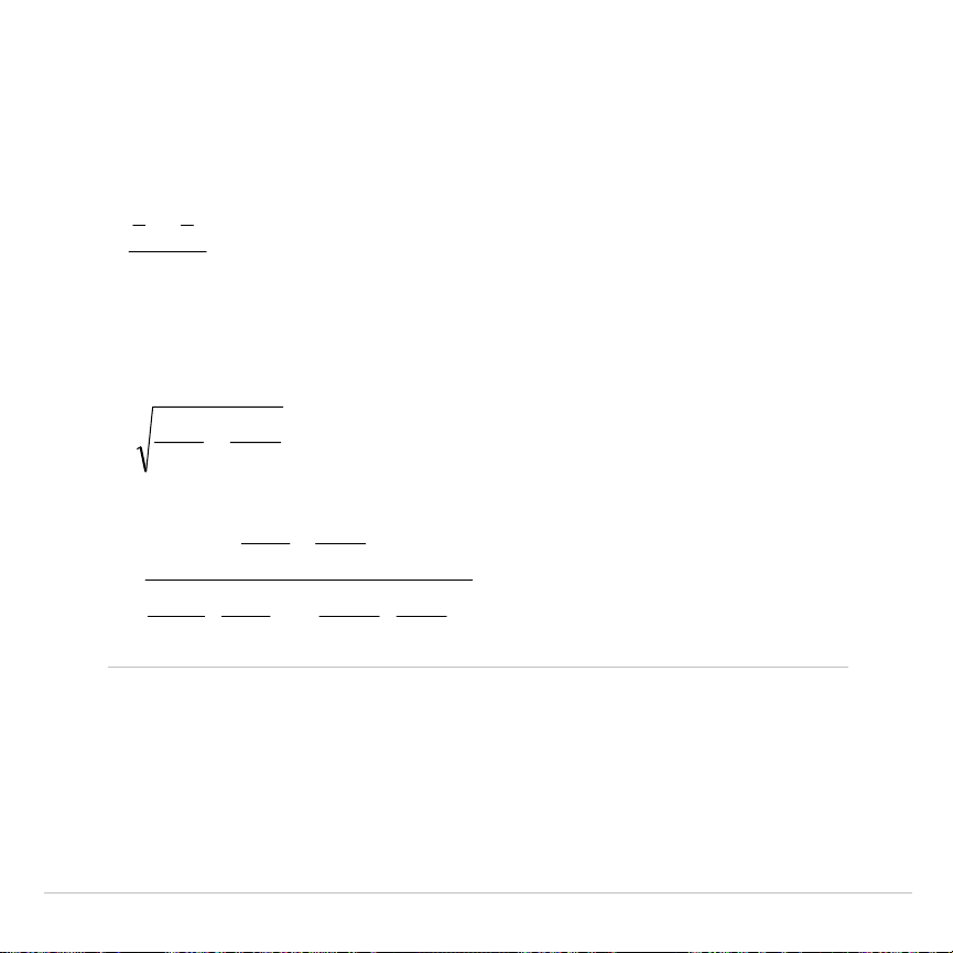
TI-83 Plus Tables and Reference Information 726
2
.
SampTTest
The following is the definition for the
2
.
SampTTest
. The two-sample
t
statistic with degrees of freedom
df
is:
S
xx
t
21
−
=
where the computation of
S
and
df
are dependent on whether the
variances are pooled. If the variances are not pooled:
2
2
2
1
2
1
n
Sx
n
Sx
S
+=
2
2
2
2
2
2
1
2
1
1
2
2
2
2
1
2
1
1
1
1
1
−
+
−
+
=
n
Sx
nn
Sx
n
n
Sx
n
Sx
df

TI-83 Plus Tables and Reference Information 727
otherwise:
df
SxnSxn
Sx
p
2
22
2
11
)1()1(
−+−
=
p
Sx
nn
S
21
11
+=
2
21
−+=
nndf
and
Sxp
is the pooled variance.

TI-83 Plus Tables and Reference Information 728
Financial Formulas
This section contains financial formulas for computing time value of
money, amortization, cash flow, interest-rate conversions, and days
between dates.
Time Value of Money
[]
1
))1(ln(
−=
+×
xy
ei
where:
PMT
ƒ
0
y
=
C/Y
÷
P/Y
x
=(.
01
×
I%
)
÷
C/Y
C/Y
= compounding periods per year
P/Y
= payment periods per year
I%
= interest rate per year
1)(
)1(
−÷=
÷−
N
PVFVi
where:
PMT
=
0
The iteration used to compute
i
:
N
N
i
iFV
i
i
GPMTPV
−
−
+×+
+−
×+=
)1(
)1(1
0

TI-83 Plus Tables and Reference Information 729
[]
1/ 100%
))1ln((
−××=
+×
xy
eYCI
where:
x=i
y = P/Y
÷
C/Y
kiG
i
×+=
1
where:
k=
0
for end-of-period payments
k=
1
for beginning-of-period payments
)1(ln
ln
i
iPVGPMT
iFVGPMT
N
i
i
+
××
×−×
=
+
where:
i
ƒ
0
PMTFVPVN
÷+=
−
)(
where:
i=
0
−+
+
+×=
−
1)1(
N
i
i
FVPV
PV
G
i
PMT

TI-83 Plus Tables and Reference Information 730
where:
i
ƒ
0
NFVPVPMT
÷+=
−
)(
where:
i=
0
i
GPMT
i
FV
i
GPMT
PV
i
N
i
×
−
+
×
−
×
=
)1(
1
where:
i
ƒ
0
)(
NPMTFVPV
×+=
−
where:
i=
0
×
+×+−
×
=
i
GPMT
PVi
i
GPMT
FV
i
N
i
)1(
where:
i
ƒ
0
)(
NPMTPVFV
×+=
−
where:
i
=
0

TI-83 Plus Tables and Reference Information 731
Amortization
If computing
bal
(),
pmt
2
=
npmt
Let
bal
(
0
) =
RND
(
PV
)
Iterate from
m
=
1
to
pmt
2
+−−=
−×=
−
)(I)1()(
))]1((12[I
m
m
PMTRNDmbalmbal
mbaliRNDRND
then:
)2()(
pmtbalbal
=
)1()2()(Pr
pmtbalpmtbaln
−=
Σ
)(Pr)()112()(
nPMTRNDpmtpmtInt
Σ−×+−=
Σ

TI-83 Plus Tables and Reference Information 732
where:
RND
= round the display to the number of decimal places
selected
RND12
= round to
12
decimal places
Balance, principal, and interest are dependent on the values of
PMT
,
PV
,
æ
, and
pmt
1
and
pmt
2
.
Cash Flow
∑
=
−
−
−
+−
++=
N
j
n
S
j
i
i
iCFCFnpv
j
j
1
0
))1(1(
)1()(
1
where:
=
≥
=
∑
=
00
1
1
j
jn
S
j
i
i
j
Net present value is dependent on the values of the initial cash flow
(
CF
0
), subsequent cash flows (
CFj
), frequency of each cash flow (
nj
),
and the specified interest rate (
i
).
irr
() =
100
×
i
, where
i
satisfies
npv
() =
0

TI-83 Plus Tables and Reference Information 733
Internal rate of return is dependent on the values of the initial cash flow
(
CF
0
) and subsequent cash flows (
CFj
).
i
=
I
%
÷
100
Interest Rate Conversions
4
Eff
=
)1(100
)1(ln
−×
+×
xCP
e
where:
x
=.
01
×
Nom
÷
CP
4
Nom
=
[]
1100
)1(ln1
−××
+×÷
xCP
eCP
where:
x
=.
01
×
Eff
Eff
=
effective rate
CP
=
compounding periods
Nom
=
nominal rate
Days between Dates
With the
dbd(
function, you can enter or compute a date within the
range Jan. 1, 1950, through Dec. 31, 2049.

TI-83 Plus Tables and Reference Information 734
Actual/actual day-count method
(assumes actual number of days per
month and actual number of days per year):
dbd
( (days between dates) = Number of Days II
-
Number of Days I
Number of Days I = (
Y1
-
YB
)
×
365
+ (number of days
MB
to
M
1
)
+
DT
1
+
4
)1(
YBY
−
Number of Days II = (
Y
2
-
YB
)
×
365
+ (number of days
MB
to
M
2
)
+
DT
2
+
4
)2(
YBY
−
where:
M
1
= month of first date
DT
1
= day of first date
Y
1
= year of first date
M
2
= month of second date
DT
2
= day of second date
Y
2
= year of second date
MB
= base month (January)
DB
= base day (
1
)
YB
= base year (first year after leap year)
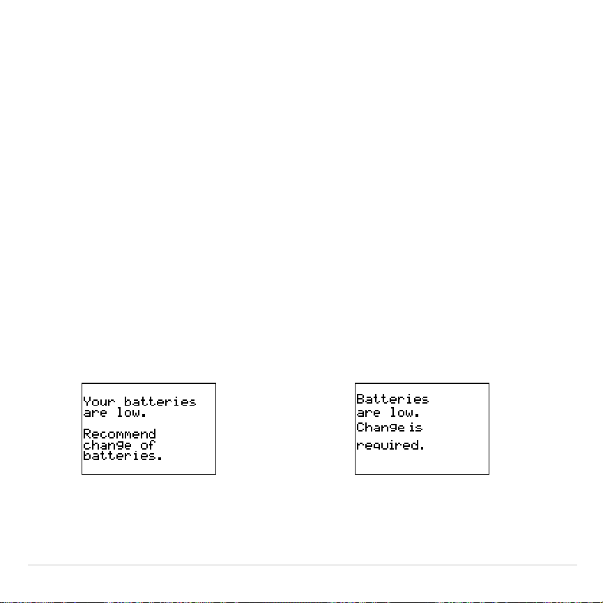
TI-83 Plus General Information 735
Appendix B:
General Information
Battery Information
When to Replace the Batteries
The TI-83 Plus uses five batteries: four AAA alkaline batteries and one
lithium battery. The lithium battery provides auxiliary power to retain
memory while you replace the AAA batteries.
When the battery voltage level drops below a usable level, the TI-83 Plus:
Displays this message when
you turn on the unit.
Displays this message when you
attempt to download an application.
Message A Message B

TI-83 Plus General Information 736
After
Message A
is first displayed, you can expect the batteries to
function for about one or two weeks, depending on usage. (This one-
week to two-week period is based on tests with alkaline batteries; the
performance of other kinds of batteries may vary.)
The low-battery message continues to be displayed each time you turn
on the unit until you replace the batteries. If you do not replace the
batteries within about two weeks, the calculator may turn off by itself or
fail to turn on until you install new batteries.
If
Message B
is displayed, you must to replace the batteries immediately
to successfully download an application.
Replace the lithium battery every three or four years.
Effects of Replacing the Batteries
Do not remove both types of batteries (AAA and lithium auxiliary) at the
same time. Do not allow the batteries to lose power completely. If you
follow these guidelines and the steps for replacing batteries, you can
replace either type of battery without losing any information in memory.

TI-83 Plus General Information 737
Battery Precautions
Take these precautions when replacing batteries.
•
Do not leave batteries within reach of children
•
Do not mix new and used batteries. Do not mix brands (or types
within brands) of batteries.
•
Do not mix rechargeable and nonrechargeable batteries.
•
Install batteries according to polarity (+ and
N
) diagrams.
•
Do not place nonrechargeable batteries in a battery recharger.
•
Properly dispose of used batteries immediately. Do not leave them
within the reach of children.
•
Do not incinerate or dismantle batteries.
Replacing the Batteries
To replace the batteries, follow these steps.
1. Turn off the calculator. Replace the slide cover over the keyboard to
avoid inadvertently turning on the calculator. Turn the back of the
calculator toward you.
2. Hold the calculator upright, push downward on the latch on the top of
the battery cover with your finger, and then pull the cover toward you.

TI-83 Plus General Information 738
Note:
To avoid loss of information stored in memory, you must turn off the
calculator. Do not remove the AAA batteries and the lithium battery
simultaneously.
3. Replace all four AAA alkaline batteries simultaneously. Or, replace
the lithium battery.
•
To replace the AAA alkaline batteries, remove all four discharged
AAA batteries and install new ones according to the polarity
(+ and
N
) diagram in the battery compartment.
•
To replace the lithium battery, remove the screw from the lithium-
battery cover, and then remove the cover. Install the new battery,
+ side up. Replace the cover and secure it with the screw. Use a
CR1616 or CR1620 (or equivalent) lithium battery.
4. Replace the battery compartment cover. Turn the calculator on and
adjust the display contrast, if necessary.

TI-83 Plus General Information 739
In Case of Difficulty
Handling a Difficulty
To handle a difficulty, follow these steps.
1. If you cannot see anything on the screen, the contrast may need to
be adjusted.
To darken the screen, press and release
y
, and then press and
hold
}
until the display is sufficiently dark.
To lighten the screen, press and release
y
, and then press and
hold
†
until the display is sufficiently light.
2. If an error menu is displayed, follow the steps in Chapter 1. Refer to
the
Error Conditions
table for details about specific errors, if
necessary.
3. If the busy indicator (dotted line) is displayed, a graph or program has
been paused; the TI-83 Plus is waiting for input. Press
Í
to
continue or press
É
to break.
4. If a checkerboard cursor (
#
) is displayed, then either you have
entered the maximum number of characters in a prompt, or memory
is full. If memory is full:

TI-83 Plus General Information 740
•
Press
y
L
2
to display the
MEMORY MANAGEMENT DELETE
menu.
•
Select the type of data you want to delete, or select
1:All
for a list
of all variables of all types. A screen is displayed listing each
variable of the type you selected and the number of bytes each
variable is using.
•
Press
}
and
†
to move the selection cursor (
4
) next to the item
you want to delete, and then press
{
. (Chapter 18).
5. If the calculator does not seem to work at all, be sure the batteries
are fresh and that they are installed properly. Refer to battery
information on pages 736 and 737.
6. If the calculator still doesn’t work even though you are sure the
batteries are sufficiently charged, you can try the two solutions in the
order they are presented.
•
Download calculator system software as follows:
a. Remove one battery from the calculator and then press and
hold the
{
key while re-installing the battery. This will force
the calculator to accept a download of system software.
b. Connect your calculator to a personal computer with the
TI
.
GRAPH LINK
™
accessory to download current or
new software code to your calculator.

TI-83 Plus General Information 741
•
II. If the above solution does not work, reset all memory as
follows:
a. Remove one battery from the calculator and then press and
hold down the
‘
key while re-installing the battery. While
continuing to hold down the
‘
key, press and hold down
the
É
key. When the home screen is displayed, release the
keys.
b. Press
y
L
to display the
MEMORY
menu.
c. Select
7:Reset
to display the
RAM ARCHIVE ALL
menu.
d. Press
~
~
to display the
ALL
menu.
e. Select
1:All Memory
to display the
RESET MEMORY
menu.
f. To continue with the reset, select
2:Reset
. The message
MEM
cleared
is displayed on the home screen.

TI-83 Plus General Information 742
Error Conditions
When the TI-83 Plus detects an error, it displays
ERR:
message
and an
error menu. Chapter 1 describes the general steps for correcting errors.
This table contains each error type, possible causes, and suggestions for
correction.
Error Type Possible Causes and Suggested Remedies
ARCHIVED
You have attempted to use, edit, or delete an archived
variable. For example, dim(L1) is an error if L1 is archived.
ARCHIVE FULL
You have attempted to archive a variable and there is not
enough space in archive to receive it.
ARGUMENT
A function or instruction does not have the correct number
of arguments. See Appendix A and the appropriate
chapter.
BAD ADDRESS
You have attempted to send or receive an application and
an error (e.g. electrical interference) has occurred in the
transmission.

TI-83 Plus General Information 743
Error Type Possible Causes and Suggested Remedies
BAD GUESS •
In a
CALC
operation, you specified a Guess that is not
between Left Bound and Right Bound.
•
For the solve( function or the equation solver, you
specified a
guess
that is not between
lower
and
upper
.
•
Your guess and several points around it are undefined.
Examine a graph of the function. If the equation has a
solution, change the bounds and/or the initial guess.
BOUND •
In a
CALC
operation or with Select(
,
you defined
Left Bound > Right Bound.
•
In fMin(, fMax(, solve(, or the equation solver, you
entered
lower
‚
upper
.
BREAK
You pressed the
É
key to break execution of a program,
to halt a
DRAW
instruction, or to stop evaluation of an
expression.

TI-83 Plus General Information 744
Error Type Possible Causes and Suggested Remedies
DATA TYPE
You entered a value or variable that is the wrong data
type.
•
For a function (including implied multiplication) or an
instruction, you entered an argument that is an invalid
data type, such as a complex number where a real
number is required. See Appendix A and the
appropriate chapter.
•
In an editor, you entered a type that is not allowed, such
as a matrix entered as an element in the stat list editor.
See the appropriate chapter.
•
You attempted to store an incorrect data type, such as a
matrix, to a list.
DIM MISMATCH
You attempted to perform an operation that
references more than one list or matrix, but the
dimensions do not match.
DIVIDE BY 0 •
You attempted to divide by zero. This error is not
returned during graphing. The TI-83 Plus allows for
undefined values on a graph.
•
You attempted a linear regression with a vertical line.

TI-83 Plus General Information 745
Error Type Possible Causes and Suggested Remedies
DOMAIN •
You specified an argument to a function or instruction
outside the valid range. This error is not returned during
graphing. The TI-83 Plus allows for undefined values on
a graph. See Appendix A and the appropriate chapter.
•
You attempted a logarithmic or power regression with a
L
X or an exponential or power regression with a
L
Y.
•
You attempted to compute
G
Prn( or
G
Int( with
pmt2
<
pmt1
.
DUPLICATE •
You attempted to create a duplicate group name.
Duplicate Name •
A variable you attempted to transmit cannot be
transmitted because a variable with that name already
exists in the receiving unit.
EXPIRED
You have attempted to run an application with a limited
trial period which has expired.

TI-83 Plus General Information 746
Error Type Possible Causes and Suggested Remedies
Error in Xmit •
The TI-83 Plus was unable to transmit an item. Check
to see that the cable is firmly connected to both units
and that the receiving unit is in receive mode.
•
You pressed
É
to break during transmission.
•
You attempted to perform a backup from a TI
.
82 to a
TI-83 Plus.
•
You attempted to transfer data (other than L
1
through
L
6
) from a TI-83 Plus to a TI
.
82.
•
You attempted to transfer L
1
through L
6
from a
TI-83 Plus to a TI
.
82 without using 5:Lists to TI82 on
the
LINK SEND
menu.
ID NOT FOUND
This error occurs when the SendID command is executed
but the proper calculator ID cannot be found.
ILLEGAL NEST •
You attempted to use an invalid function in an argument
to a function, such as seq( within
expression
for seq(.
INCREMENT •
The increment in seq( is 0 or has the wrong sign. This
error is not returned during graphing. The TI-83 Plus
allows for undefined values on a graph.
•
The increment in a For( loop is 0.

TI-83 Plus General Information 747
Error Type Possible Causes and Suggested Remedies
INVALID •
You attempted to reference a variable or use a function
where it is not valid. For example, Y
n
cannot reference
Y, Xmin,
@
X, or TblStart.
•
You attempted to reference a variable or function that
was transferred from the TI
.
82 and is not valid for the
TI-83 Plus. For example, you may have transferred
U
n
N
1 to the TI-83 Plus from the TI
.
82 and then tried to
reference it.
•
In Seq mode, you attempted to graph a phase plot
without defining both equations of the phase plot.
•
In Seq mode, you attempted to graph a recursive
sequence without having input the correct number of
initial conditions.
•
In Seq mode, you attempted to reference terms other
than (
n
N
1) or (
n
N
2).
•
You attempted to designate a graph style that is invalid
within the current graph mode.
•
You attempted to use Select( without having selected
(turned on) at least one xyLine or scatter plot.

TI-83 Plus General Information 748
Error Type Possible Causes and Suggested Remedies
INVALID DIM
•
You specified dimensions for an argument that are not
appropriate for the operation.
•
You specified a list dimension as something other than
an integer between 1 and 999.
•
You specified a matrix dimension as something other
than an integer between 1 and 99.
•
You attempted to invert a matrix that is not square.
ITERATIONS
•
The solve( function or the equation solver has
exceeded the maximum number of permitted iterations.
Examine a graph of the function. If the equation has a
solution, change the bounds, or the initial guess, or
both.
•
irr( has exceeded the maximum number of permitted
iterations.
•
When computing
æ
, the maximum number of iterations
was exceeded.
LABEL
The label in the Goto instruction is not defined with a Lbl
instruction in the program.

TI-83 Plus General Information 749
Error Type Possible Causes and Suggested Remedies
MEMORY
Memory is insufficient to perform the instruction or
function. You must delete items from memory (Chapter 18)
before executing the instruction or function.
Recursive problems return this error; for example,
graphing the equation Y
1
=Y
1
.
Branching out of an If/Then, For(, While, or Repeat loop
with a Goto also can return this error because the End
statement that terminates the loop is never reached.
MemoryFull
•
You are unable to transmit an item because the
receiving unit’s available memory is insufficient. You
may skip the item or exit receive mode.
•
During a memory backup, the receiving unit’s available
memory is insufficient to receive all items in the sending
unit’s memory. A message indicates the number of
bytes the sending unit must delete to do the memory
backup. Delete items and try again.
MODE
You attempted to store to a window variable in another
graphing mode or to perform an instruction while in the
wrong mode; for example, DrawInv in a graphing mode
other than Func.

TI-83 Plus General Information 750
Error Type Possible Causes and Suggested Remedies
NO SIGN CHNG
•
The solve( function or the equation solver did not
detect a sign change.
•
You attempted to compute
æ
when FV, (
Úä
PMT), and
PV are all
‚
0, or when FV, (
Úä
PMT), and PV are all
0.
•
You attempted to compute irr( when neither
CFList
nor
CFO
is
>
0, or when neither
CFList
nor
CFO
is
<
0.
NONREAL ANS
In Real mode, the result of a calculation yielded a complex
result. This error is not returned during graphing. The
TI-83 Plus allows for undefined values on a graph.
OVERFLOW
You attempted to enter, or you have calculated, a number
that is beyond the range of the calculator. This error is not
returned during graphing. The TI-83 Plus allows for
undefined values on a graph.
RESERVED
You attempted to use a system variable inappropriately.
See Appendix A.
SINGULAR MAT
•
A singular matrix (determinant = 0) is not valid as the
argument for
L
1
.
•
The SinReg instruction or a polynomial regression
generated a singular matrix (determinant = 0) because
it could not find a solution, or a solution does not exist.
This error is not returned during graphing. The TI-83 Plus
allows for undefined values on a graph.

TI-83 Plus General Information 751
Error Type Possible Causes and Suggested Remedies
SINGULARITY
expression
in the solve( function or the equation solver
contains a singularity (a point at which the function is not
defined). Examine a graph of the function. If the equation
has a solution, change the bounds or the initial guess or
both.
STAT
You attempted a stat calculation with lists that are not
appropriate.
•
Statistical analyses must have at least two data points.
•
Med
.
Med must have at least three points in each
partition.
•
When you use a
frequency list, its elements must be
‚
0.
•
(Xmax
N
Xmin)
à
Xscl must be
47 for a histogram.
STAT PLOT
You attempted to display a graph when a stat plot that
uses an undefined list is turned on.
SYNTAX
The command contains a syntax error. Look for misplaced
functions, arguments, parentheses, or commas. See
Appendix A and the appropriate chapter.
TOL NOT MET
You requested a tolerance to which the algorithm cannot
return an accurate result.

TI-83 Plus General Information 752
Error Type Possible Causes and Suggested Remedies
UNDEFINED
You referenced a variable that is not currently defined. For
example, you referenced a stat variable when there is no
current calculation because a list has been edited, or you
referenced a variable when the variable is not valid for the
current calculation, such as a after Med
.
Med.
VALIDATION
Electrical interference caused a link to fail or this calculator
is not authorized to run the application.
VARIABLE
You have tried to archive a variable that cannot be
archived or you have have.tried to unarchive an application
or group.
Examples of variables that cannot be archived include:
•
Real numbers LRESID, R, T, X, Y, Theta, Statistic
variables under Vars, STATISTICS menu, Yvars, and
the AppIdList.
VERSION
You have attempted to receive an incompatible variable
version from another calculator.

TI-83 Plus General Information 753
Error Type Possible Causes and Suggested Remedies
WINDOW RANGE
A problem exists with the window variables.
•
You defined Xmax
Xmin or Ymax
Ymin.
•
You defined
q
max
q
min and
q
step > 0 (or vice
versa).
•
You attempted to define Tstep=0.
•
You defined Tmax
Tmin and Tstep > 0 (or vice
versa).
•
Window variables are too small or too large to graph
correctly. You may have attempted to zoom in or zoom
out to a point that exceeds the TI-83 Plus’s numerical
range.
ZOOM
•
A point or a line, instead of a box, is defined in ZBox.
•
A
ZOOM
operation returned a math error.

TI-83 Plus General Information 754
Accuracy Information
Computational Accuracy
To maximize accuracy, the TI-83 Plus carries more digits internally than
it displays. Values are stored in memory using up to 14 digits with a two-
digit exponent.
•
You can store a value in the window variables using up to 10 digits
(12 for
Xscl
,
Yscl
,
Tstep
, and
q
step
).
•
Displayed values are rounded as specified by the mode setting with a
maximum of 10 digits and a two-digit exponent.
•
RegEQ
displays up to 14 digits in
Float
mode. Using a fixed-decimal
setting other than
Float
causes
RegEQ
results to be rounded and
stored with the specified number of decimal places.
Xmin
is the center of the leftmost pixel,
Xmax
is the center of the next-to-
the-rightmost pixel. (The rightmost pixel is reserved for the busy
indicator.)
@
X
is the distance between the centers of two adjacent pixels.
•
In
Full
screen mode,
@
X
is calculated as (
Xmax
N
Xmin
)
à
94. In
G
.
T
split-screen mode,
@
X
is calculated as (
Xmax
N
Xmin
)
à
46.
•
If you enter a value for
@
X
from the home screen or a program in
Full
screen mode,
Xmax
is calculated as
Xmin
+
@
X
…
94. In
G
.
T
split-
screen mode,
Xmax
is calculated as
Xmin
+
@
X
…
46.

TI-83 Plus General Information 755
Ymin
is the center of the next-to-the-bottom pixel;
Ymax
is the center of
the top pixel.
@
Y
is the distance between the centers of two adjacent
pixels.
•
In
Full
screen mode,
@
Y
is calculated as (
Ymax
N
Ymin
)
à
62. In
Horiz
split-screen mode,
@
Y
is calculated as (
Ymax
N
Ymin
)
à
30. In
G
.
T
split-screen mode,
@
Y
is calculated as (
Ymax
N
Ymin
)
à
50.
•
If you enter a value for
@
Y
from the home screen or a program in
Full
screen mode,
Ymax
is calculated as
Ymin
+
@
Y
…
62. In
Horiz
split-
screen mode,
Ymax
is calculated as
Ymin
+
@
Y
…
30. In
G
.
T
split-
screen mode,
Ymax
is calculated as
Ymin
+
@
Y
…
50.
Cursor coordinates are displayed as eight-character numbers (which
may include a negative sign, decimal point, and exponent) when
Float
mode is selected.
X
and
Y
are updated with a maximum accuracy of
eight digits.
minimum
and
maximum
on the
CALCULATE
menu are calculated with a
tolerance of 1
E
L
5;
‰
f(x)dx
is calculated at 1
E
L
3. Therefore, the result
displayed may not be accurate to all eight displayed digits. For most
functions, at least five accurate digits exist. For
fMin(
,
fMax(
, and
fnInt(
on the
MATH
menu and
solve(
in the
CATALOG
, the tolerance can be
specified.

TI-83 Plus General Information 756
Function Limits
Function Range of Input Values
sin
x
,
cos
x
,
tan
x
0
|
x
| < 10
12
(radian or degree)
sin
L
1
x
,
cos
L
1
x
L
1
x
1
ln
x
,
log
x
10
L
100
<
x
< 10
100
e
x
L
10
100
<
x
230.25850929940
10
x
L
10
100
<
x
< 100
sinh
x
,
cosh
x
|
x
|
230.25850929940
tanh
x
|
x
| < 10
100
sinh
L
1
x
|
x
| < 5 × 10
99
cosh
L
1
x
1
x
< 5 × 10
99
tanh
L
1
x
L
1 <
x
< 1
‡
x
(real mode) 0
x
< 10
100
‡
x
(complex mode) |
x
| < 10
100
x
!
L
.5
x
69, where
x
is a multiple of .5

TI-83 Plus General Information 757
Function Results
Function Range of Result
sin
L
1
x
,
tan
L
1
x
L
90
¡
to 90
¡
or
Lpà
2 to
pà
2 (radians)
cos
L
1
x
0
¡
to 180
¡
or 0 to
p
(radians)

TI-83 Plus General Information 758
Support and Service Information
Product Support
Customers in the U.S., Canada, Puerto Rico, and the Virgin Islands
For general questions, contact Texas Instruments Customer Support:
phone:
1
.
800
.
TI
.
CARES (1
.
800
.
842
.
2737)
e-mail:
For technical questions, call the Programming Assistance Group of
Customer Support:
phone:
1
.
972
.
917
.
8324
Customers outside the U.S., Canada, Puerto Rico, and the Virgin
Islands
Contact TI by e-mail or visit the TI calculator home page on the World
Wide Web.
e-mail:
Internet:
education.ti.com

TI-83 Plus General Information 759
Product Service
Customers in the U.S. and Canada Only
Always contact Texas Instruments Customer Support before returning a
product for service.
Customers outside the U.S. and Canada
Refer to the leaflet enclosed with this product or contact your local Texas
Instruments retailer/distributor.
Other TI Products and Services
Visit the TI calculator home page on the World Wide Web.
Internet:
education.ti.com
Refer to the leaflet enclosed with this product or contact your local Texas
Instruments retailer/distributor.

TI-83 Plus General Information 760
Warranty Information
Customers in the U.S. and Canada Only
One-Year Limited Warranty for Electronic Product
This Texas Instruments (“TI”) electronic product warranty extends only to the
original purchaser and user of the product.
Warranty Duration. This TI electronic product is warranted to the original
purchaser for a period of one (1) year from the original purchase date.
Warranty Coverage. This TI electronic product is warranted against defective
materials and construction.
THIS WARRANTY IS VOID IF THE PRODUCT HAS BEEN
DAMAGED BY ACCIDENT OR UNREASONABLE USE, NEGLECT, IMPROPER
SERVICE, OR OTHER CAUSES NOT ARISING OUT OF DEFECTS IN MATERIALS OR
CONSTRUCTION.
Warranty Disclaimers.
ANY IMPLIED WARRANTIES ARISING OUT OF THIS SALE,
INCLUDING BUT NOT LIMITED TO THE IMPLIED WARRANTIES OF
MERCHANTABILITY AND FITNESS FOR A PARTICULAR PURPOSE, ARE LIMITED IN
DURATION TO THE ABOVE ONE-YEAR PERIOD. TEXAS INSTRUMENTS SHALL NOT
BE LIABLE FOR LOSS OF USE OF THE PRODUCT OR OTHER INCIDENTAL OR
CONSEQUENTIAL COSTS, EXPENSES, OR DAMAGES INCURRED BY THE
CONSUMER OR ANY OTHER USER.
Some states/provinces do not allow the exclusion or limitation of implied
warranties or consequential damages, so the above limitations or exclusions
may not apply to you.

TI-83 Plus General Information 761
Legal Remedies.
This warranty gives you specific legal rights, and you may
also have other rights that vary from state to state or province to province.
Warranty Performance.
During the above one (1) year warranty period, your
defective product will be either repaired or replaced with a reconditioned model
of an equivalent quality (at TI’s option) when the product is returned, postage
prepaid, to Texas Instruments Service Facility. The warranty of the repaired or
replacement unit will continue for the warranty of the original unit or six (6)
months, whichever is longer. Other than the postage requirement, no charge
will be made for such repair and/or replacement. TI strongly recommends that
you insure the product for value prior to mailing.
Software.
Software is licensed, not sold. TI and its licensors do not warrant that
the software will be free from errors or meet your specific requirements.
All
software is provided “AS IS.”
Copyright.
The software and any documentation supplied with this product are
protected by copyright.
Australia & New Zealand Customers only
One-Year Limited Warranty for Commercial Electronic Product
This Texas Instruments electronic product warranty extends only to the original
purchaser and user of the product.
Warranty Duration.
This Texas Instruments electronic product is warranted to
the original purchaser for a period of one (1) year from the original purchase
date.

TI-83 Plus General Information 762
Warranty Coverage.
This Texas Instruments electronic product is warranted
against defective materials and construction. This warranty is void if the product
has been damaged by accident or unreasonable use, neglect, improper service,
or other causes not arising out of defects in materials or construction.
Warranty Disclaimers. Any implied warranties arising out of this sale,
including but not limited to the implied warranties of merchantability and
fitness for a particular purpose, are limited in duration to the above one-
year period. Texas Instruments shall not be liable for loss of use of the
product or other incidental or consequential costs, expenses, or damages
incurred by the consumer or any other user.
Some jurisdictions do not allow the exclusion or limitation of implied warranties
or consequential damages, so the above limitations or exclusions may not
apply to you.
Legal Remedies.
This warranty gives you specific legal rights, and you may
also have other rights that vary from jurisdiction to jurisdiction.
Warranty Performance.
During the above one (1) year warranty period, your
defective product will be either repaired or replaced with a new or reconditioned
model of an equivalent quality (at TI’s option) when the product is returned to
the original point of purchase. The repaired or replacement unit will continue for
the warranty of the original unit or six (6) months, whichever is longer. Other
than your cost to return the product, no charge will be made for such repair
and/or replacement. TI strongly recommends that you insure the product for
value if you mail it.

TI-83 Plus General Information 763
Software:
Software is licensed, not sold. TI and its licensors do not warrant that
the software will be free from errors or meet your specific requirements. All
software is provided “
AS IS
.”
Copyright:
The software and any documentation supplied with this product are
protected by copyright.
All Customers Outside the U.S. and Canada
For information about the length and terms of the warranty, refer to your
package and/or to the warranty statement enclosed with this product, or contact
your local Texas Instruments retailer/distributor.

TI-83 Plus Index 764
Index
!
(factorial), 94, 692
" "
(string indicator), 484
"
(seconds notation), 97, 697
æ
(annual interest rate variable), 444,
462
¡
(degrees notation), 692
à
(division), 63, 696
å
(exponent), 14, 20, 661
ì
(graph style, animate), 117
í
(graph style, dot), 117
ç
(graph style, line), 117
‚
(greater than or equal to), 101, 694
(less than or equal to), 101, 694
ä
(multiplication), 63, 695
M
(negation), 49, 66, 695
ƒ
(not equal to), 101, 694
Ú
(number of payment periods
variable), 444, 462
p
(pi), 66
Ö
(plot type, box), 371
Ò
(plot type, histogram), 370
Õ
(plot type, modified box), 370
Ô
(plot type, normal probability), 372
N
(subtraction), 63, 696
¨
(user-created list name symbol), 309,
668
!
Store, 29, 686
‡
(
(square root), 64, 695
›
,
¦
(pixel mark), 235, 373
L
1
(inverse), 64, 271, 694
c
2
.
Test
(chi-square test), 412, 657
c
2
cdf(
(chi-square cdf), 429, 657
c
2
pdf(
(chi-square pdf), 428, 657
Û
cdf(
, 430, 662
4
Dec
(to decimal conversion), 67, 659
!
dim(
(assign dimension), 275, 301,
660
¨
DIST
, 471
4
DMS
(to degrees/minutes/seconds), 99,
661
¨
DREF
, 471
4
Eff(
(to effective interest rate), 459,
662
‰
f(x)dx
operation on a graph, 153
4
Frac
(to fraction), 67, 664
G
Int(
(sum of interest), 455, 668
¨
LIGHT
, 471
@
List(
, 303, 669
¨
LREF
, 471
4
Nom(
(to nominal interest rate), 459,
672
Û
pdf(
, 429, 664
4
Polar
(to polar), 91, 675
G
Prn(
(sum of principal), 455, 676

TI-83 Plus Index 765
4
Rect
(to rectangular), 91, 679
…
row(
, 282, 680
…
row+(
, 282, 680
@
Tbl
(table step variable), 205
¨
TEMP
, 471
¨
TREF
, 471
¨
VOLT
, 471
¨
VREF
, 471
@
X
window variable, 124
@
Y
window variable, 124
'
(minutes notation), 97, 697
( ) (parentheses), 48
+
(addition), 63, 696
+
(concatenation), 490, 696
+
(pixel mark), 235, 373
:
(colon), 504
<
(less than), 101, 694
=
(equal-to relational test), 101, 693
>
(greater than), 101, 694
[ ]
(matrix indicator), 265
^
(power), 64, 695
{ }
(list indicator), 288
1
.
PropZInt
(one-proportion z confidence
interval), 410, 676
1
.
PropZTest
(one-proportion z test),
402, 676
1
.
Var Stats
(one-variable statistics),
357, 689
10
^(
(power of ten), 65, 695
2
(square), 64, 694
2
.
PropZInt
(two-proportion z
confidence interval), 411, 676
2
.
PropZTest
(two-proportion z test),
403, 677
2
.
Samp
Û
Test
(two-sample
Û
-Test), 414,
681
2
.
SampTInt
(two-sample t confidence
interval), 408, 681
2
.
SampTTest
(two-sample t test), 400,
682
2
.
SampZInt
(two-sample z confidence
interval), 407, 682
2
.
SampZTest
(two-sample z test), 399,
682
2
.
Var Stats
(two-variable statistics),
358, 689
3
(cube), 68, 693
3
‡
(
(cube root), 68, 693
—A—
a+b
i
(rectangular complex mode), 24,
84, 656
about, 596
above graph style(
é
), 117
abs(
(absolute value), 79, 90, 271, 655
accuracy information
computational and graphing, 754
function limits and results, 756
graphing, 132

TI-83 Plus Index 766
addition (
+
), 63, 696
alpha cursor, 12
alpha-lock, 18
alternative hypothesis, 391
amortization
G
Int(
(sum of interest), 455, 668
G
Prn(
(sum of principal), 455, 676
bal(
(amortization balance), 454,
656
calculating schedules, 454
formula, 731
and
(Boolean operator), 103, 655
ANGLE
menu, 97
angle modes, 22
angle(
, 90, 655
animate graph style (
ì
), 117
ANOVA(
(one-way variance analysis),
417, 655
formula, 722
Ans
(last answer), 36, 599, 655
APD (Automatic Power Down), 6
applications. See examples,
applications
Apps
, 27, 598
AppVars
, 27, 598
arccosine (
cos
L
1
(
), 63
Archive
, 30, 610, 655
archive full error, 628, 742
garbage collection, 623
memory error, 623
archived variables, 719
arcsine (
sin
L
1
(
), 63
arctangent (
tan
L
1
(
), 63
Asm(
, 537, 655
AsmComp(
, 537, 655
AsmPrgm(
, 537, 655
assembly language programs, 537
augment(
, 277, 307, 656
Automatic Power Down (APD), 6
automatic regression equation, 353
automatic residual list (
RESID
), 352
axes format, sequence graphing, 187
axes, displaying (AxesOn, AxesOff),
127, 656
AxesOff
, 127, 656
AxesOn
, 127, 656
—B—
backing up calculator memory, 638,
650
bal(
(amortization balance), 454, 656
bar, 468
batteries, 7, 735
below graph style (
ê
), 117
binomcdf(
, 431, 656
binompdf(
, 430, 656
block, 623
Boolean logic, 103
box pixel mark (
›
), 235, 373

TI-83 Plus Index 767
Boxplot
plot type (
Ö
), 371
busy indicator, 11
—C—
C/Y
(compounding-periods-per-year
variable), 444, 463
CALCULATE
menu, 147
Calculate
output option, 388, 392
cash flow
calculating, 452
formula, 732
irr(
(internal rate of return), 453, 668
npv(
(net present value), 453, 673
CATALOG
, 481
CBL 2/CBL, 464
CBL/CBR
Quitting, 480
Running, 464
Selecting, 464
CBL/CBR APP
menu, 467
CBR, 464, 533, 633, 665
check memory
, 596
chi-square cdf (
c
2
cdf(
), 429, 657
chi-square pdf (
c
2
pdf(
), 428, 657
chi-square test (
c
2
.
Test
), 412, 657
Circle(
(draw circle), 228, 657
Clear Entries
, 596, 657
clearing
all lists (
ClrAllLists
), 596, 657
drawing (
ClrDraw
), 217, 657
entries (
Clear Entries
), 596, 657
home screen (
ClrHome
), 532, 657
list (
ClrList
), 349, 658
table (
ClrTable
), 532, 658
ClrAllLists
(clear all lists), 596, 657
ClrDraw
(clear drawing), 217, 657
ClrHome
(clear home screen), 532, 657
ClrList
(clear list), 349, 658
ClrTable
(clear table), 532, 658
coefficients of determination (
r
2
,
R
2
,
354
colon separator (
:
), 504
combinations (
nCr
), 93, 672
compiling an assembly program, 537,
655
complex
modes (
a+b
i
, r
e
^
q
i
), 24, 84, 656,
679
numbers, 24, 84, 679
compounding-periods-per-year variable
(
C/Y
), 444, 463
concatenation (
+
), 490, 696
confidence intervals, 392
conj(
(conjugate), 88, 658
Connected
(plotting mode), 23, 658
connecting two calculators, 633
contrast (display), 8
convergence, sequence graphing, 195
conversions

TI-83 Plus Index 768
4
Dec
(to decimal), 67, 659
4
DMS
(to degrees/minutes/ seconds),
99, 661
4
Eff
(to effective interest rate), 459
4
Frac
(to fraction conversion), 67,
664
4
Nom
(to nominal interest rate
conversion), 459, 672
4
Polar
(to polar conversion), 91, 675
4
Rect
(to rectangular conversion),
91, 679
Equ
4
String(
(equation-to-string
conversion), 491, 662
List
4
matr(
(list-to-matrix
conversion), 279, 308, 670
Matr
4
list(
(matrix-to-list conversion),
278, 308, 670
P
4
Rx(
,
P
4
Ry(
(polar-to-rectangular
conversion), 100, 678
R
4
Pr(
,
R
4
P
q
(
(rectangular-to-polar
conversion), 100, 681
String
4
Equ(
(string-to-equation
conversion), 493, 686
CoordOff
, 126, 658
CoordOn
, 126, 658
correlation coefficient (
r
), 354
cos
L
1
(
(arccosine), 63, 658
cos(
(cosine), 63, 658
cosh
M
1
(
(hyperbolic arccosine), 496, 658
cosh(
(hyperbolic cosine), 496, 658
cosine (
cos(
), 63, 658
cross pixel mark (
+
), 235, 373
cube (
3
), 68, 693
cube root (
3
‡
(
), 68, 693
cubic regression (
CubicReg
), 359, 658
CubicReg
(cubic regression), 359, 658
cumSum(
(cumulative sum), 279, 303,
659
cumulative sum (
cumSum(
), 279, 303,
659
cursors, 12, 18
—D—
data collection
methods, 468
options, 468
results, 471
starting & stopping, 479
Data input option, 388, 390
data logger, 473
data points, 475
data results, 471
days between dates (
dbd(
), 460, 659,
733
dbd(
(days between dates), 460, 659,
733
decimal mode (float or fixed), 21
decrement and skip (
DS<(
), 521, 661
definite integral, 70, 152, 165

TI-83 Plus Index 769
defragmenting, 622
Degree
angle mode, 22, 97, 659
degrees notation (
¡
), 98, 692
delete variable contents (
DelVar
), 523,
659
deleting items from memory
, 599
DelVar
(delete variable contents), 659
DependAsk
, 206, 209, 659
DependAuto
, 206, 209, 659
derivative. See numerical derivative
det(
(determinant), 275, 659
determinant (
det(
), 275, 659
DiagnosticOff
, 354, 660
DiagnosticOn
, 354, 660
diagnostics display mode(
r
r
2
,
R
2
), 354
differentiation, 72, 152, 165, 175
dim(
(dimension), 275, 301, 660
dimensioning a list or matrix, 275, 301,
660
directions, 471
DIRECTNS
, 471
Disp
(display), 528, 529, 660
DispGraph
(display graph), 530, 660
display contrast, 8
display cursors, 12
DispTable
(display table), 530, 661
DISTR
(distributions menu), 424
DISTR DRAW
(distributions drawing
menu), 434
distribution functions
c
2
cdf(
, 429, 657
c
2
pdf(
, 428, 657
Û
cdf(
, 430, 662
Û
pdf(
, 429, 664
binomcdf(
, 431, 656
binompdf(
, 430, 656
geometcdf(
, 433, 665
geometpdf(
, 433, 665
invNorm(
, 426, 668
normalcdf(
, 426, 672
normalpdf(
, 425, 673
poissoncdf(
, 432, 675
poissonpdf(
, 432, 675
tcdf(
, 427, 687
tpdf(
, 427, 687
distribution shading instructions
Shade
Û
(
, 437, 684
Shade
c
2
(
, 436, 684
Shade_t(
, 435, 684
ShadeNorm(
, 435, 684
division (
à
), 63, 696
DMS (degrees/minutes/seconds entry
notation), 97, 697
Dot
(plotting mode), 23, 661
dot graph style (
í
), 117
dot pixel mark (
¦
), 235, 373
dr/d
q
operation on a graph, 175
DRAW
menu, 214
Draw output option, 388, 392
DRAW POINTS
menu, 233

TI-83 Plus Index 770
DRAW STO
(draw store menu), 239
DrawF
(draw a function), 224, 661
drawing on a graph
circles (
Circle(
), 228
line segments (
Line(
), 218
lines (
Horizontal
,
Line(
,
Vertical
),
221
pixels (
Pxl
.
Change
,
Pxl
.
Off
,
Pxl
.
On
,
pxl
.
Test)
, 237
points
(
Pt
.
Change
,
Pt
.
Off
,
Pt
.
On)
,
233
tangents (
Tangent
), 222
text (
Text
), 230
using
Pen
, 232
DrawInv
(draw inverse), 224, 661
DS<(
(decrement and skip), 521, 661
DuplicateName
menu, 644
dx/dt
operation on a graph, 152, 165
dy/dx
operation on a graph, 152, 165,
175
—E—
e (constant), 65
e^(
(exponential), 65, 661
edit keys table, 17
Else
, 514
End
, 476, 515, 662
Eng
(engineering notation mode), 20,
662
ENTRY
(last entry key), 33
entry cursor, 12
EOS (Equation Operating System), 47
eqn
(equation variable), 72
Equ
4
String(
(equation-to-string
conversion), 491, 662
equal-to relational test (
=
), 101, 693
Equation Operating System (EOS), 47
Equation Solver
, 72
equations with multiple roots, 77
errors
diagnosing and correcting, 59
messages, 742
examples—applications
area between curves, 578
areas of regular n-sided polygons,
588
box plots, 560
box with lid, 546
defining a, 546
defining a table of values, 547
finding calculated maximum, 557
setting the viewing window, 551
tracing the graph, 553
zooming in on the graph, 555
zooming in on the table, 549
cobweb attractors, 572
fundamental theorem of calculus,
584
guess the coefficients, 574

TI-83 Plus Index 771
inequalities, 566
mortgage payments, 592
parametric equations, ferris wheel
problem, 580
piecewise functions, 564
quadratic formula
converting to a fraction, 542
displaying complex results, 544
entering a calculation, 540
Sierpinski triangle, 570
solving a system of nonlinear
equations, 568
unit circle and trig curves, 576
examples—Getting Started
coin flip, 61
compound interest, 442
drawing a tangent line, 212
financing a car, 440
forest and trees, 176
generating a sequence, 283
graphing a circle, 105
mean height of a population, 381
path of a ball, 154
pendulum lengths and periods, 315
polar rose, 166
roots of a function, 203
sending variables, 629
solving a system of linear equations,
256
unit circle, 246
volume of a cylinder, 497
examples—miscellaneous
calculating outstanding loan
balances, 456
convergence, 195
daylight hours in Alaska, 363
predator-prey model, 197
exponential regression (
ExpReg
), 361,
662
expr(
(string-to-expression conversion),
491, 662
ExpReg
(exponential regression), 361,
662
expression, 13
converting from string (
expr(
), 491,
662
turning on and off (
ExprOn
, 128,
662
ExprOff
(expression off), 128, 662
ExprOn
(expression on), 128, 662
—F—
factorial (
!
), 94, 692
family of curves, 131
Fill(
, 276, 663
FINANCE CALC
menu, 446
FINANCE VARS
menu, 462
financial functions
amortization schedules, 454

TI-83 Plus Index 772
cash flows, 452
days between dates, 460
interest rate conversions, 459
payment method, 461
time value of money (
TVM
), 448
Fix
(fixed-decimal mode), 21, 663
fixed-decimal mode (
Fix
), 21, 663
Float
(floating-decimal mode), 21, 663
floating-decimal mode (
Float
), 21, 663
fMax(
(function maximum), 69, 663
fMin(
(function minimum), 69, 663
fnInt(
(function integral), 71, 663
FnOff
(function off), 115, 663
FnOn
(function on), 115, 664
For(
, 515, 664
format settings, 125, 187
formulas
amortization, 731
ANOVA
, 722
cash flow, 732
days between dates, 733
factorial, 94
interest rate conversions, 733
logistic regression, 721
sine regression, 722
time value of money, 728
two-sample
Û
-Test, 724
two-sample t test, 726
fPart(
(fractional part), 80, 273, 664
free-moving cursor, 132
frequency, 357
Full
(full-screen mode), 25, 664
full-screen mode (
Full
), 25, 664
Func
(function graphing mode), 23, 664
function graphing
@
X
and
@
Y
window variables, 124
accuracy, 132
CALC
(calculate menu), 147
defining and displaying, 107
defining in the
Y=
editor, 111
defining on the home screen, in a
program, 112
deselecting, 114, 115
displaying, 108, 121, 129
evaluating, 113
family of curves, 131
format settings, 125
free-moving cursor, 132
graph styles, 117
maximum of (
fMax(
), 69, 663
minimum of (
fMin(
), 663
modes, 23, 109, 664
moving the cursor to a value, 135
overlaying functions on a graph,
130
panning, 136
pausing or stopping a graph, 129
Quick Zoom, 136
selecting, 114, 115, 664
shading, 119

TI-83 Plus Index 773
Smart Graph, 129
tracing, 134
viewing window, 121
window variables, 121, 122, 123
Y=
editor, 111
ZOOM MEMORY
menu, 144
ZOOM
menu, 138
function integral (
fnInt(
), 71, 663
function, definition of, 15
functions and instructions table, 654
future value, 444, 451
FV
(future-value variable), 444, 462
—G—
G
.
T
(graph-table split-screen mode), 25,
252, 666
garbage collecting, 622
GarbageCollect
, 626, 664
Gauge, 468
gcd(
(greatest common divisor), 82, 665
GDB
(graph database), 242
geometcdf(
, 433, 665
geometpdf(
, 433, 665
Get(
(get data from CBL 2/CBL or
CBR), 533, 665
GetCalc(
(get data from TI
.
83), 533,
665
getKey
, 531, 665
Getting Started. See examples, Getting
Started
Goto
, 519, 665
graph database (
GDB
), 242
graph styles, 117
graphing modes, 23
graphing-order modes, 24
GraphStyle(
, 524, 665
graph-table split-screen mode (
G
.
T
), 25,
252, 666
greater than (
>
), 101, 694
greater than or equal to (
‚
), 101, 694
greatest common divisor (
gcd(
), 82, 665
greatest integer (
int(
), 81, 273, 668
GridOff
, 127, 666
GridOn
, 127, 666
grouping, 616
—H—
Histogram
plot type (
Ò
), 370
home screen, 10
Horiz
(horizontal split-screen mode),
25, 250, 666
Horizontal
(draw line), 221, 666
hyperbolic functions, 495
hypothesis tests, 396
—I—
i
(complex number constant), 86

TI-83 Plus Index 774
identity(
, 277, 666
If
instructions
If
, 512, 666
If-Then
, 513, 666
If-Then-Else
, 514, 667
imag(
(imaginary part), 89, 667
imaginary part (
imag(
), 89, 667
implied multiplication, 48
increment and skip (
IS>(
), 520, 668
independent variable, 206, 209, 667
IndpntAsk
, 206, 209, 667
IndpntAuto
, 206, 209, 667
inferential stat editors, 388
inferential statistics. See stat tests;
confidence intervals
alternative hypotheses, 391
bypassing editors, 393
calculating test results (
Calculate
),
392
confidence interval calculations, 392
data input or stats input, 390
entering argument values, 390
graphing test results (
Draw
), 392
input descriptions table, 419
pooled option, 391
STAT TESTS
menu, 394
test and interval output variables,
422
Input
, 526, 527, 667
insert cursor, 12
inString(
(in string), 492, 667
instruction, definition of, 16
int(
(greatest integer), 81, 273, 668
integer part (
iPart(
), 80, 273, 668
integral. See numerical integral
interest rate conversions
4
Eff(
(compute effective interest
rate), 459
4
Nom(
(compute nominal interest
rate), 459
calculating, 459
formula, 733
internal rate of return (
irr(
), 453, 668
intersect
operation on a graph, 151
INTRVL (SEC)
, 475
inverse (
L
1
), 64, 271, 694
inverse cumulative normal distribution
(
invNorm(
), 426, 668
inverse trig functions, 63
invNorm(
(inverse cumulative normal
distribution), 426, 668
iPart(
(integer part), 80, 273, 668
irr(
(internal rate of return), 453, 668
IS>(
(increment and skip), 520, 668
—K—
keyboard
layout, 2
math operations, 63

TI-83 Plus Index 775
key-code diagram, 532
—L—
LabelOff
, 127, 668
LabelOn
, 127, 668
labels
graph, 127, 668
program, 519, 669
Last Entry, 33
Lbl
(label), 519, 669
lcm(
(least common multiple), 82, 669
least common multiple (
lcm(
), 82, 669
length(
of string, 492, 669
less than (
<
), 101, 694
less than or equal to (
), 101, 694
Light-Time, 468
line graph style (
ç
), 117
line segments, drawing, 218
Line(
(draw line), 220, 669
lines, drawing, 220, 221
LINK RECEIVE
menu, 644
LINK SEND
menu, 634
linking
receiving items, 644
to a CBL 2/CBL or CBR, 633
to a PC or Macintosh, 633
to a TI
.
82, 641, 646
transmitting items, 629
two TI
.
83 Plus units, 638
LinReg(a+bx)
(linear regression), 360,
669
LinReg(ax+b)
(linear regression), 359,
669
LinRegTTest
(linear regression t test),
415, 669
LIST MATH
menu, 311
LIST NAMES
menu, 291
LIST OPS
menu, 299
List
4
matr(
(lists-to-matrix conversion),
279, 308, 670
lists
accessing an element, 289
attaching formulas, 293, 294, 336
clearing all elements, 333
copying, 289
creating, 286, 332
deleting from memory, 289, 599
detaching formulas, 296, 340
dimension, 288
entering list names, 292, 330
indicator (
{ }
), 288
naming lists, 286
storing and displaying, 288
transmitting to and from TI
.
73, 642
transmitting to and from TI
.
82, 641,
646
using in expressions, 297
using to graph a family of curves,
131, 290

TI-83 Plus Index 776
using to select data points from a
plot, 305
using with math operations, 63, 298
ln(
, 65, 670
LnReg
(logarithmic regression), 360,
670
log(
, 65, 670
logic (Boolean) operators, 103
Logistic
(regression), 361, 670
logistic regression formula, 721
—M—
marked for deletion, 623
MATH CPX
(complex menu), 88
MATH
menu, 67
MATH NUM
(number menu), 79
math operations, 63
MATH PRB
(probability menu), 92
Matr
4
list(
(matrix-to-list conversion),
278, 308, 670
matrices
accessing elements, 268
copying, 267
defined, 258
deleting from memory, 261
dimensions, 259, 275, 276
displaying a matrix, 267
displaying matrix elements, 260
editing matrix elements, 262
indicator (
[ ]
), 265
inverse (
L
1
), 271
math functions, 269
matrix math functions (
det(
,
T
,
dim(
,
Fill(
,
identity(
,
randM(
,
augment(
,
Matr
4
list(
,
List
4
matr(
,
cumSum(
),
274
referencing in expressions, 265
relational operations, 272
row operations(
ref(
,
rref(
,
rowSwap(
,
row+(
,
†
row(
,
†
row+(
), 280
selecting, 258
viewing, 261
MATRX EDIT
menu, 258
MATRX MATH
menu, 274
MATRX NAMES
menu, 265
max
, 470
max(
(maximum), 81, 311, 670
maximum of a function (
fMax(
), 69, 663
maximum
operation on a graph, 150
mean(
, 312, 671
Med
.
Med
(median-median), 358, 671
median(
, 312, 671
Mem Mgmt/Del
menu, 597
memory
backing up, 650
checking available, 596
clearing all list elements from, 602
clearing entries from, 601
deleting items from, 599

TI-83 Plus Index 777
error, 626
insufficient during transmission, 653
resetting defaults, 604
resetting memory, 604
MEMORY
menu, 596
Menu(
(define menu), 521, 671
menus, 39, 40
defining (
Menu(
), 521, 671
map, 698
scrolling, 41
meter, 468
min
, 470
min(
(minimum), 81, 311, 671
minimum of a function (
fMin(
), 69, 663
minimum
operation on a graph, 150
minutes notation (
'
), 97, 697
ModBoxplot
plot type (
Õ
), 370
mode settings, 19
a+b
i
(complex rectangular), 24, 84,
656
Connected
(plotting), 23, 658
Degree
(angle), 22, 99, 659
Dot
(plotting), 23, 661
Eng
(notation), 20, 662
Fix
(decimal), 21, 663
Float
(decimal), 21, 663
Full
(screen), 25, 664
Func
(graphing), 23, 664
G
.
T
(screen), 25, 666
Horiz
(screen), 25, 666
Normal
(notation), 20, 672
Par
/
Param
(graphing), 23, 674
Pol
/
Polar
(graphing), 23, 675
Radian
(angle), 22, 99, 678
r
e
^
q
i
(complex polar), 24, 84, 679
Real
, 24, 679
Sci
(notation), 20, 683
Seq
(graphing), 23, 683
Sequential
(graphing order), 24, 683
Simul
(graphing order), 24, 685
modified box plot type (
Õ
), 370
multiple entries on a line, 14
multiplication (
ä
), 63, 695
multiplicative inverse, 64
—N—
nCr
(number of combinations), 93, 672
nDeriv(
(numerical derivative), 70, 672
negation (
M
), 49, 66, 695
nonrecursive sequences, 182
normal distribution probability
(
normalcdf(
), 426, 672
Normal
notation mode, 20, 672
normal probability plot type (
Ô
), 372
normalcdf(
(normal distribution
probability), 426, 672
normalpdf(
(probability density
function), 425, 673
NormProbPlot
plot type (
Ô
), 372

TI-83 Plus Index 778
not equal to (
ƒ
), 101, 694
not(
(Boolean operator), 104, 673
nPr
(permutations), 93, 673
npv(
(net present value), 453, 673
numerical derivative, 70, 152, 165, 175
numerical integral, 70, 153
—O—
Omit
, 619, 645
ON/HALT
, 480
one-proportion z confidence interval
(
1
.
PropZInt
), 410, 676
one-proportion z test (
1
.
PropZTest
),
402, 676
one-sample t confidence interval
(
TInterval
), 406, 687
one-variable statistics (
1
.
Var Stats
),
357, 689
or
(Boolean) operator, 103, 673
order of evaluating equations, 47
Output(
, 255, 530, 673
Overwrite
, 619, 645
Overwrite All
, 619
—P—
P
4
Rx(
,
P
4
Ry(
(polar-to-rectangular
conversions), 100, 678
P/Y
(number-of-payment-periods-per-
year variable), 444, 463
panning, 136
Par
/
Param
(parametric graphing mode),
23, 674
parametric equations, 159
parametric graphing
CALC
(calculate operations on a
graph), 165
defining and editing, 158, 159
free-moving cursor, 163
graph format, 161
graph styles, 159
moving the cursor to a value, 164
selecting and deselecting, 160
setting parametric mode, 158
tracing, 163
window variables, 160
Y=
editor, 158
zoom operations, 165
parentheses, 48
path (
ë
) graph style, 117
Pause
, 518, 674
pausing a graph, 129
Pen
, 232
permutations (
nPr
), 93, 673
phase plots, 197
Pi (
p
), 66
Pic
(pictures), 239
pictures (
Pic
), 239
pixel, 237
pixels in
Horiz
/
G
.
T
modes, 238, 254

TI-83 Plus Index 779
PLOT
, 476
Plot1(
, 373, 674
Plot2(
, 373, 674
Plot3(
, 373, 674
PlotsOff
, 375, 675
PlotsOn
, 375, 675
plotting modes, 23
plotting stat data, 368
PMT
(payment amount variable), 444,
462
Pmt_Bgn
(payment beginning variable),
461, 675
Pmt_End
(payment end variable), 461,
675
poissoncdf(
, 432, 675
poissonpdf(
, 432, 675
Pol
/
Polar
(polar graphing mode), 23,
168, 675
polar equations, 169
polar form, complex numbers, 87
polar graphing
CALC
(calculate operations on a
graph), 175
defining and displaying, 168
equations, 169
free-moving cursor, 173
graph format, 171
graph styles, 169
mode (
Pol
/
Polar
), 23, 168, 675
moving the cursor to a value, 174
selecting and deselecting, 169
tracing, 173
window variables, 170
Y=
editor, 168
ZOOM
operations, 174
PolarGC
(polar graphing coordinates),
126, 676
pooled option, 388, 391
power (
^
), 64, 695
power of ten (
10
^(
), 65, 695
present value, 444, 450
previous entry (Last Entry), 33
prgm
(program name), 522, 676
PRGM CTL
(program control menu),
511
PRGM EDIT
menu, 510
PRGM EXEC
menu, 510
PRGM I/O
(Input/Output menu), 525
PRGM NEW
menu, 500
probability, 92
probability density function
(
normalpdf(
), 425, 673
probe, 468
prod(
(product), 313, 676
programming
copying and renaming, 509
creating new, 500
defined, 500
deleting, 501
deleting command lines, 508

TI-83 Plus Index 780
editing, 507
entering command lines, 504
executing, 505
inserting command lines, 508
instructions, 511
name (
prgm
), 522, 676
renaming, 509
running assembly language
program, 537
stopping, 506
subroutines, 535
Prompt
, 528, 676
Pt
.
Change(
, 235, 677
Pt
.
Off(
, 234, 677
Pt
.
On(
, 233, 677
PV
(present value variable), 444, 462
p-value, 422
PwrReg
(power regression), 361, 677
Pxl
.
Change(
, 237, 677
Pxl
.
Off(
, 237, 677
Pxl
.
On(
, 237, 677
pxl
.
Test(
, 238, 678
—Q—
QuadReg
(quadratic regression), 359,
678
QuartReg
(quartic regression), 360, 678
Quick Zoom, 136
Quit
, 619, 645
quitting CBL/CBR, 480
—R—
r
(correlation coefficient), 354
r
(radian notation), 99, 692
R
4
Pr(
,
R
4
P
q
(
(rectangular-to-polar
conversions), 100, 681
r
2
,
R
2
(coefficients of determination),
354
Radian
angle mode, 22, 99, 678
radian notation (
r
), 99, 692
RAM ARCHIVE ALL
menu, 603
rand
(random number), 92, 678
randBin(
(random binomial), 96, 678
randInt(
(random integer), 95, 679
randM(
(random matrix), 277, 679
randNorm(
(random Normal), 95, 679
random seed, 92
Ranger, 468
RCL
(recall), 31, 297
r
e
^
q
i
(polar complex mode), 24, 84,
679
Real
mode, 24, 679
real(
(real part), 89, 679
RealTme
, 476
RecallGDB
, 244, 679
RecallPic
, 241, 679
rectangular form, complex numbers, 86

TI-83 Plus Index 781
RectGC
(rectangular graphing
coordinates), 126, 680
recursive sequences, 183
ref(
(row-echelon form), 280, 680
reference#, 471
RegEQ
(regression equation variable),
353, 599
regression model
automatic regression equation, 353
automatic residual list feature, 352
diagnostics display mode, 354
models, 357
relational operations, 101, 272
Repeat
, 517, 680
RESET MEMORY
menu, 608
resetting
all memory, 608
archive memory, 606
defaults, 604
memory, 604
RAM memory, 604
residual list (
RESID
), 352
Return
, 523, 680
root (
x
‡
), 69, 693
root of a function, 148
round(
, 80, 271, 680
row+(
, 680
rowSwap(
, 281, 680
rref(
(reduced-row-echelon form), 280,
681
—S—
samples (# of), 475
Scatter
plot type (
"
), 369
Sci
(scientific notation mode), 20, 683
scientific notation, 14
screen modes, 25
second cursor (
2nd
), 12
second key (
2nd
), 4
seconds DMS notation (
"
), 97
sector, 623
Select(
, 304, 683
selecting
data points from a plot, 305
functions from the home screen or a
program, 115
functions in the
Y=
editor, 115
stat plots from the
Y=
editor, 115
Send(
(send to CBL 2/CBL or CBR),
533, 683
SendID, 634
sending. See transmitting
SendOS, 635
Seq
(sequence graphing mode), 23, 683
seq(
(sequence), 302, 683
sequence graphing
axes format, 187
CALC
(calculate menu), 191
defining and displaying, 179
evaluating, 192

TI-83 Plus Index 782
free-moving cursor, 189
graph format, 188
graph styles, 181
moving the cursor to a value, 190
nonrecursive sequences, 182
phase plots, 197
recursive sequences, 183
selecting and deselecting, 181
setting sequence mode, 179
TI
.
83 Plus versus TI
.
82 table, 202
tracing, 189
web plots, 193
window variables, 185
Y=
editor, 180
ZOOM
(zoom menu), 191
Sequential
(graphing order mode), 24,
683
service information, 759
setting
display contrast, 8
graph styles, 118
graph styles from a program, 120
modes, 20
modes from a program, 20
split-screen modes, 248
split-screen modes from a program,
255
tables from a program, 206
SetUpEditor
, 350, 683
shade above (
é
) graph style, 117
shade below (
ê
) graph style, 117
Shade
Û
(
, 437, 684
Shade
c
2
(
, 436, 684
Shade(
, 226, 684
Shade_t(
, 435, 684
ShadeNorm(
, 435, 684
shading graph areas, 119, 226
Simul
(simultaneous graphing order
mode), 24, 685
sin
L
1
(
(arcsine), 63, 685
sin(
(sine), 63, 685
sine (
sin(
), 63, 685
sine regression formula, 722
sinh
M
1
(
(hyperbolic arcsine), 496, 685
sinh(
(hyperbolic sine), 496, 685
SinReg
(sinusoidal regression), 362,
685
Smart Graph, 129
solve(
, 77, 685
Solver
, 72
solving for variables in the equation
solver, 75
sonic, 468
sonic probe, 468
sonic-time graph, 468
SortA(
(sort ascending), 299, 348, 685
SortD(
(sort descending), 299, 348, 685
split-screen modes
G
.
T
(graph-table) mode, 252
Horiz
(horizontal) mode, 250

TI-83 Plus Index 783
setting, 248, 255
split-screen values, 231, 238, 254
square (
2
), 64, 694
square root (
‡
(
), 64, 695
STAT CALC
menu, 356
STAT EDIT
menu, 348
stat list editor
attaching formulas to list names,
336
clearing elements from lists, 333
creating list names, 332
detaching formulas from list names,
340
displaying, 329
edit-elements context, 344
editing elements of formula-
generated lists, 341
editing list elements, 334
entering list names, 330
enter-names context, 346
formula-generated list names, 338
removing lists, 332
restoring list names
L
1
–
L
6
, 333
switching contexts, 342
view-elements context, 344
view-names context, 346
STAT PLOTS
menu, 373
stat tests and confidence intervals
c
²
.
Test
(chi-square test), 412
1
.
PropZInt
(one-proportion z
confidence interval), 410
1
.
PropZTest
(one-proportion z test),
402
2
.
PropZInt
(two-proportion z
confidence interval), 411
2
.
PropZTest
(two-proportion z test),
403
2
.
Samp
Û
Test
(two-sample
Û
.
Test),
414
2
.
SampTInt
(two-sample t
confidence interval), 408
2
.
SampTTest
(two-sample t test),
400
2
.
SampZInt
(two-sample z
confidence interval), 407
2
.
SampZTest
(two-sample z test),
399
ANOVA(
(one-way analysis of
variance), 415
LinRegTTest
(linear regression t
test), 415
T
.
Test
(one-sample t test), 397
TInterval
(one-sample t confidence
interval), 406
Z
.
Test
(one-sample z test), 396
ZInterval
(one-sample z confidence
interval), 405
STAT TESTS
menu, 394

TI-83 Plus Index 784
statistical distribution functions. See
distribution functions
statistical plotting, 368
Boxplot
(regular box plot), 371
defining, 373
from a program, 378
Histogram
, 370
ModBoxplot
(modified box plot),
370
NormProbPlot
(normal probability
plot), 372
Scatter
, 369
tracing, 376
turning on/off stat plots, 115, 375
viewing window, 376
xyLine
, 369
statistical variables table, 365
Stats input option, 388, 390
stdDev(
(standard deviation), 314, 686
Stop
, 523, 686
Store (
!
), 29, 686
StoreGDB
, 242, 686
StorePic
, 239, 686
storing
graph databases (
GDB
s), 242
graph pictures, 239
variable values, 29
String
4
Equ(
(string-to-equation
conversions), 493, 686
strings
concatenation (
+
), 490, 696
converting, 491
defined, 484
displaying contents, 488
entering, 484
functions in
CATALOG
, 489
length (
length(
), 492, 669
storing, 487
variables, 486, 487
student-t distribution
probability (
tcdf(
), 427, 687
probability density function (
tpdf(
),
427, 687
sub(
(substring), 493, 686
subroutines, 522
subtraction (
N
), 63, 696
sum(
(summation), 313, 686
system variables, 719
—T—
T
(transpose matrix), 275, 693
T
.
Test
(one-sample t test), 397, 688
TABLE SETUP
screen, 205
tables
description, 209
variables, 205, 207
tan
L
1
(
(arctangent), 63, 686
tan(
(tangent), 63, 686
tangent (
tan(
), 63, 686

TI-83 Plus Index 785
tangent lines, drawing, 222
Tangent(
(draw line), 222, 687
tanh
M
1
(
(hyperbolic arctangent), 496,
687
tanh(
(hyperbolic tangent), 496, 687
TblStart
(table start variable), 205
tcdf(
(student-t distribution probability),
427, 687
technical support, 758
Temperature, 468
Temp-Time, 468
TEST
(relational menu), 101
TEST LOGIC
(Boolean menu), 103
Text(
instruction, 230, 254, 687
placing on a graph, 230, 254
Then
, 513, 666
thick (
è
) graph style, 117
TI
.
82
link differences, 646
transmitting to/from, 644
TI
.
83
Link. See linking
TI
.
83 Plus
key code diagram, 532
keyboard, 2
menu map, 698
TI Connect
, 632
TI
.
GRAPH LINK
, 632, 633
Time
axes format, 187, 687
time value of money (
TVM
)
æ
variable (annual interest rate),
462
Ú
variable (number of payment
periods), 462
C/Y
variable (number of
compounding periods per year),
463
calculating, 448
formulas, 728
FV
variable (future value), 462
P/Y
variable (number of payment
periods per year), 463
PMT
variable (payment amount),
462
PV
variable (present value), 462
TVM Solver
, 444
tvm_
Ú
(# payment periods), 450,
688
tvm_FV
(future value), 451, 688
tvm_I%
(interest rate), 449, 688
tvm_Pmt
(payment amount), 449,
688
tvm_PV
(present value), 450, 688
variables, 462
TInterval
(one-sample t confidence
interval), 406, 687
tpdf(
(student-t distribution probability
density function), 427, 687
TRACE
cursor, 135

TI-83 Plus Index 786
entering numbers during, 135, 164,
173, 189
expression display, 128, 135
Trace
instruction in a program, 137,
688
transmitting
error conditions, 652
from a TI
.
73 to a TI
.
83 Plus, 648
from a TI
.
82 to a TI
.
83 Plus, 646
lists to a TI
.
73, 642
lists to a TI
.
82, 641
lists to a TI
.
83 Plus, 648
stopping, 637
to an additional TI
.
83 Plus, 638
transpose matrix
(
T
), 275, 693
TRIGGER
, 480
trigonometric functions, 63
turning on and off
axes, 127
calculator, 6
coordinates, 126
expressions, 128
functions, 115
grid, 127
labels, 127
pixels, 237
points, 233
stat plots, 115, 375
tvm_
Ú
(# payment periods), 450, 688
tvm_FV
(future value), 451, 688
tvm_I%
(interest rate), 449, 688
tvm_Pmt
(payment amount), 449, 688
tvm_PV
(present value), 450, 688
two-proportion z confidence interval
(
2
.
PropZInt
), 411, 676
two-proportion z test (
2
.
PropZTest
),
403, 677
two-sample
Û
-Test formula, 724
two-sample t test formula, 726
two-variable statistics (
2
.
Var Stats
),
358, 689
Type
Bar or Meter, 469
—U—
u
sequence function, 179
UnArchive
, 30, 610, 689
ungrouping, 616
units, 470
user variables, 718
uv
/
uvAxes
(axes format), 187, 689
uw
/
uwAxes
(axes format), 187, 689
—V—
v
sequence function, 179
value
operation on a graph, 147
variables
complex, 26
displaying and storing values, 30

TI-83 Plus Index 787
equation solver, 75
graph databases, 26
graph pictures, 26
independent/dependent, 209
list, 26, 286
matrix, 26, 258
real, 26
recalling values, 31
solver editor, 74
statistical, 365
string, 486, 487
test and interval output, 422
types, 26
user and system, 27, 718
VARS
and
Y
.
VARS
menus, 44
variance of a list (
variance(
), 314, 689
variance(
(variance of a list), 314, 689
VARS
menu
GDB
, 44
Picture
, 44
Statistics
, 44
String
, 44
Table
, 44
Window
, 44
Zoom
, 44
Vertical
(draw line), 221, 689
viewing window, 121
Volt, 468
Voltage, 468
Volt-Time, 468
vw
/
uvAxes
(axes format), 187, 689
—W—
w
sequence function, 179
warranty information, 760
Web
(axes format), 187, 689
web plots, 193
While
, 516, 689
window variables
function graphing, 121
parametric graphing, 161
polar graphing, 170
—X—
x
‡
(root), 69, 693
XFact
zoom factor, 145
x-intercept of a root, 148
xor
(Boolean) exclusive or operator,
103, 690
x
th
root (
x
‡
), 69
xyLine
(
Ó
) plot type, 369
—Y—
Y
.
VARS
menu
Function
, 45
On/Off
, 45
Parametric
, 45
Polar
, 45

TI-83 Plus Index 788
Y=
editor
function graphing, 111
parametric graphing, 158
polar graphing, 168
sequence graphing, 180
YFact
zoom factor, 145
—Z—
Z
.
Test
(one-sample z test), 396, 692
ZBox
, 139, 690
ZDecimal
, 141, 690
zero
operation on a graph, 148
ZInteger
, 143, 690
ZInterval
(one-sample z confidence
interval), 405, 690
zoom, 138, 139, 140, 141, 142, 143,
144, 145, 146
cursor, 139
factors, 145
function graphing, 138
parametric graphing, 165
polar graphing, 174
sequence graphing, 191
Zoom In
(zoom in), 140, 690
ZOOM MEMORY
menu, 144
ZOOM
menu, 138
Zoom Out
(zoom out), 140, 690
ZoomFit
(zoom to fit function), 143,
691
ZoomRcl
(recall stored window), 145,
691
ZoomStat
(statistics zoom), 143, 691
ZoomSto
(store zoom window), 144,
691
ZPrevious
(use previous window), 144,
691
ZSquare
(set square pixels), 142, 691
ZStandard
(use standard window), 142,
691
ZTrig
(trigonometric window), 142, 692

TI-83 Plus Quick-Find Locator i
Quick-Find Locator
Chapter 1: Operating the TI-83 Plus Silver Edition........................ 1
Documentation Conventions.....................................................................1
TI-83 Plus Keyboard.................................................................................2
Keyboard Zones..................................................................................2
Using the Color
.
Coded Keyboard.......................................................4
Using the
y
and
ƒ
Keys...........................................................4
Turning On and Turning Off the TI-83 Plus ..............................................6
Turning On the Calculator...................................................................6
Turning Off the Calculator...................................................................7
Batteries..............................................................................................7
Setting the Display Contrast .....................................................................8
Adjusting the Display Contrast............................................................8
When to Replace Batteries.................................................................9
The Display.............................................................................................10
Types of Displays..............................................................................10
Home Screen....................................................................................10
Displaying Entries and Answers .......................................................10
Returning to the Home Screen .........................................................11
Busy Indicator...................................................................................11
Display Cursors.................................................................................12
Entering Expressions and Instructions....................................................13
What Is an Expression?....................................................................13
Entering an Expression.....................................................................13
Multiple Entries on a Line..................................................................14

TI-83 Plus Quick-Find Locator ii
Entering a Number in Scientific Notation..........................................14
Functions ..........................................................................................15
Instructions........................................................................................16
Interrupting a Calculation..................................................................16
TI-83 Plus Edit Keys ...............................................................................17
Setting Modes.........................................................................................19
Checking Mode Settings...................................................................19
Changing Mode Settings...................................................................20
Setting a Mode from a Program........................................................20
Normal, Sci, Eng...............................................................................20
Float, 0123456789............................................................................21
Radian, Degree.................................................................................22
Func, Par, Pol, Seq...........................................................................23
Connected, Dot.................................................................................23
Sequential, Simul..............................................................................24
Real, a+b
i
, re^
q
i
................................................................................24
Full, Horiz, G-T..................................................................................25
Using TI-83 Plus Variable Names...........................................................26
Variables and Defined Items.............................................................26
Notes about Variables.......................................................................27
Storing Variable Values ..........................................................................29
Storing Values in a Variable..............................................................29
Displaying a Variable Value..............................................................30
Archiving Variables (Archive, Unarchive)..........................................30
Recalling Variable Values.......................................................................31
Using Recall (RCL)...........................................................................31
ENTRY (Last Entry) Storage Area..........................................................33
Using ENTRY (Last Entry)................................................................33

TI-83 Plus Quick-Find Locator iii
Accessing a Previous Entry..............................................................34
Reexecuting the Previous Entry........................................................34
Multiple Entry Values on a Line ........................................................35
Clearing ENTRY ...............................................................................36
Using Ans in an Expression..............................................................36
Continuing an Expression.................................................................37
Storing Answers................................................................................38
TI-83 Plus Menus....................................................................................39
Using a TI-83 Plus Menu ..................................................................39
Displaying a Menu ............................................................................40
Moving from One Menu to Another...................................................41
Scrolling a Menu...............................................................................41
Selecting an Item from a Menu.........................................................41
Leaving a Menu without Making a Selection.....................................43
VARS and VARS Y-VARS Menus..........................................................44
VARS Menu......................................................................................44
Selecting a Variable from the VARS Menu or VARS Y-VARS
Menu...........................................................................................45
Equation Operating System (EOS).........................................................47
Order of Evaluation...........................................................................47
Implied Multiplication.........................................................................48
Parentheses......................................................................................48
Negation............................................................................................49
Special Features of the TI-83 Plus .........................................................50
Flash – Electronic Upgradability .......................................................50
1.56 Megabytes (M) of Available Memory ........................................50
Applications.......................................................................................51
Archiving...........................................................................................51

TI-83 Plus Quick-Find Locator iv
Calculator-Based Laboratory™ (CBL 2™, CBL™) and
Calculator-Based Ranger™ (CBR™)..........................................52
Other TI-83 Plus Features......................................................................53
Graphing...........................................................................................53
Sequences........................................................................................53
Tables...............................................................................................54
Split Screen.......................................................................................54
Matrices ............................................................................................54
Lists...................................................................................................55
Statistics............................................................................................55
Inferential Statistics...........................................................................55
Applications.......................................................................................56
CATALOG.........................................................................................56
Programming ....................................................................................57
Archiving...........................................................................................57
Communication Link .........................................................................57
Error Conditions......................................................................................59
Diagnosing an Error..........................................................................59
Correcting an Error ...........................................................................60
Chapter 2: Math, Angle, and Test Operations.............................. 61
Getting Started: Coin Flip .......................................................................61
Keyboard Math Operations.....................................................................63
Using Lists with Math Operations .....................................................63
+ (Addition),
N
(Subtraction),
ä
(Multiplication),
à
(Division)...............63
Trigonometric Functions ...................................................................63
^ (Power),
2
(Square),
‡
( (Square Root) ..........................................64
L
1
(Inverse)........................................................................................64

TI-83 Plus Quick-Find Locator v
log(, 10^(, ln(.....................................................................................65
e^( (Exponential).................................................................................65
e (Constant)......................................................................................65
L
(Negation).......................................................................................66
p
(Pi) .................................................................................................66
MATH Operations...................................................................................67
MATH Menu......................................................................................67
4
Frac,
4
Dec........................................................................................67
3
(Cube),
3
‡
( (Cube Root) .................................................................68
x
‡
(Root)...........................................................................................69
fMin(, fMax(.......................................................................................69
nDeriv( ..............................................................................................70
fnInt(..................................................................................................71
Using the Equation Solver ......................................................................72
Solver................................................................................................72
Entering an Expression in the Equation Solver.................................72
Entering and Editing Variable Values ...............................................74
Solving for a Variable in the Equation Solver....................................75
Editing an Equation Stored to eqn....................................................77
Equations with Multiple Roots...........................................................77
Further Solutions...............................................................................77
Controlling the Solution for Solver or solve(......................................78
Using solve( on the Home Screen or from a Program......................78
MATH NUM (Number) Operations..........................................................79
MATH NUM Menu.............................................................................79
abs(...................................................................................................79
round(................................................................................................80
iPart(, fPart(.......................................................................................80

TI-83 Plus Quick-Find Locator vi
int( ....................................................................................................81
min(, max(.........................................................................................81
lcm(, gcd(..........................................................................................82
Entering and Using Complex Numbers...................................................84
Complex-Number Modes..................................................................84
Entering Complex Numbers..............................................................85
Note about Radian Versus Degree Mode.........................................85
Interpreting Complex Results............................................................86
Rectangular-Complex Mode.............................................................86
Polar-Complex Mode........................................................................87
MATH CPX (Complex) Operations.........................................................88
MATH CPX Menu .............................................................................88
conj(..................................................................................................88
real(...................................................................................................89
imag(.................................................................................................89
angle(................................................................................................90
abs(...................................................................................................90
4
Rect.................................................................................................91
4
Polar................................................................................................91
MATH PRB (Probability) Operations.......................................................92
MATH PRB Menu .............................................................................92
rand...................................................................................................92
nPr, nCr.............................................................................................93
! (Factorial)........................................................................................94
randInt(..............................................................................................95
randNorm(.........................................................................................95
randBin( ............................................................................................96
ANGLE Operations.................................................................................97

TI-83 Plus Quick-Find Locator vii
ANGLE Menu....................................................................................97
Entry Notation...................................................................................97
¡
(Degree) .........................................................................................98
r
(Radians)........................................................................................99
8
DMS................................................................................................99
R
8
Pr(, R
8
P
q
(, P
8
Rx(, P
8
Ry(........................................................100
TEST (Relational) Operations...............................................................101
TEST Menu.....................................................................................101
=,
ƒ
, >,
‚
, <,
..................................................................................101
Using Tests.....................................................................................102
TEST LOGIC (Boolean) Operations .....................................................103
TEST LOGIC Menu.........................................................................103
Boolean Operators..........................................................................103
and, or, xor......................................................................................103
not(..................................................................................................104
Using Boolean Operations..............................................................104
Chapter 3: Function Graphing..................................................... 105
Getting Started: Graphing a Circle........................................................105
Defining Graphs....................................................................................107
TI-83 Plus—Graphing Mode Similarities.........................................107
Defining a Graph.............................................................................107
Displaying and Exploring a Graph ..................................................108
Saving a Graph for Later Use.........................................................108
Setting the Graph Modes......................................................................109
Checking and Changing the Graphing Mode..................................109
Setting Modes from a Program.......................................................110
Defining Functions................................................................................111

TI-83 Plus Quick-Find Locator viii
Displaying Functions in the Y= Editor.............................................111
Defining or Editing a Function.........................................................111
Defining a Function from the Home Screen or a Program..............112
Evaluating Y= Functions in Expressions.........................................113
Selecting and Deselecting Functions....................................................114
Selecting and Deselecting a Function.............................................114
Turning On or Turning Off a Stat Plot in the Y= Editor....................115
Selecting and Deselecting Functions from the Home Screen
or a Program.............................................................................115
Setting Graph Styles for Functions.......................................................117
Graph Style Icons in the Y= Editor..................................................117
Setting the Graph Style...................................................................118
Shading Above and Below..............................................................119
Setting a Graph Style from a Program............................................120
Setting the Viewing Window Variables .................................................121
The TI-83 Plus Viewing Window.....................................................121
Displaying the Window Variables....................................................121
Changing a Window Variable Value ...............................................122
Storing to a Window Variable from the Home Screen or a
Program ....................................................................................123
@
X and
@
Y........................................................................................124
Setting the Graph Format.....................................................................125
Displaying the Format Settings.......................................................125
Changing a Format Setting.............................................................125
RectGC, PolarGC ...........................................................................126
CoordOn, CoordOff.........................................................................126
GridOff, GridOn...............................................................................127
AxesOn, AxesOff ............................................................................127

TI-83 Plus Quick-Find Locator ix
LabelOff, LabelOn...........................................................................127
ExprOn, ExprOff..............................................................................128
Displaying Graphs ................................................................................129
Displaying a New Graph.................................................................129
Pausing or Stopping a Graph..........................................................129
Smart Graph ...................................................................................129
Overlaying Functions on a Graph...................................................130
Graphing a Family of Curves..........................................................131
Exploring Graphs with the Free-Moving Cursor....................................132
Free-Moving Cursor........................................................................132
Graphing Accuracy .........................................................................132
Exploring Graphs with TRACE..............................................................134
Beginning a Trace...........................................................................134
Moving the Trace Cursor ................................................................134
Moving the Trace Cursor from Function to Function.......................135
Moving the Trace Cursor to Any Valid X Value...............................135
Panning to the Left or Right............................................................136
Quick Zoom.....................................................................................136
Leaving and Returning to TRACE...................................................137
Using TRACE in a Program............................................................137
Exploring Graphs with the ZOOM Instructions......................................138
ZOOM Menu...................................................................................138
Zoom Cursor...................................................................................139
ZBox................................................................................................139
Zoom In, Zoom Out.........................................................................140
ZDecimal.........................................................................................141
ZSquare..........................................................................................142
ZStandard.......................................................................................142

TI-83 Plus Quick-Find Locator x
ZTrig................................................................................................142
ZInteger...........................................................................................143
ZoomStat ........................................................................................143
ZoomFit...........................................................................................143
Using ZOOM MEMORY........................................................................144
ZOOM MEMORY Menu..................................................................144
ZPrevious........................................................................................144
ZoomSto .........................................................................................144
ZoomRcl..........................................................................................145
ZOOM FACTORS...........................................................................145
Checking XFact and YFact.............................................................145
Changing XFact and YFact.............................................................146
Using ZOOM MEMORY Menu Items from the Home Screen
or a Program.............................................................................146
Using the CALC (Calculate) Operations...............................................147
CALCULATE Menu.........................................................................147
value ...............................................................................................147
zero.................................................................................................148
minimum, maximum........................................................................150
intersect ..........................................................................................151
dy/dx ...............................................................................................152
‰
f(x)dx..............................................................................................153
Chapter 4: Parametric Graphing ................................................. 154
Getting Started: Path of a Ball ..............................................................154
Defining and Displaying Parametric Graphs.........................................158
TI-83 Plus Graphing Mode Similarities ...........................................158
Setting Parametric Graphing Mode.................................................158

TI-83 Plus Quick-Find Locator xi
Displaying the Parametric Y= Editor...............................................158
Selecting a Graph Style..................................................................159
Defining and Editing Parametric Equations ....................................159
Selecting and Deselecting Parametric Equations...........................160
Setting Window Variables...............................................................160
Setting the Graph Format ...............................................................161
Displaying a Graph .........................................................................161
Window Variables and Y
.
VARS Menus..........................................161
Exploring Parametric Graphs................................................................163
Free-Moving Cursor........................................................................163
TRACE............................................................................................163
Moving the Trace Cursor to Any Valid T Value...............................164
ZOOM.............................................................................................165
CALC ..............................................................................................165
Chapter 5: Polar Graphing........................................................... 166
Getting Started: Polar Rose..................................................................166
Defining and Displaying Polar Graphs..................................................168
TI-83 Plus Graphing Mode Similarities ...........................................168
Setting Polar Graphing Mode..........................................................168
Displaying the Polar Y= Editor........................................................168
Selecting Graph Styles ...................................................................169
Defining and Editing Polar Equations .............................................169
Selecting and Deselecting Polar Equations....................................169
Setting Window Variables...............................................................170
Setting the Graph Format ...............................................................171
Displaying a Graph .........................................................................171
Window Variables and Y
.
VARS Menus..........................................171

TI-83 Plus Quick-Find Locator xii
Exploring Polar Graphs.........................................................................173
Free-Moving Cursor........................................................................173
TRACE............................................................................................173
Moving the Trace Cursor to Any Valid
q
Value...............................174
ZOOM.............................................................................................174
CALC ..............................................................................................175
Chapter 6: Sequence Graphing................................................... 176
Getting Started: Forest and Trees........................................................176
Defining and Displaying Sequence Graphs..........................................179
TI-83 Plus Graphing Mode Similarities ...........................................179
Setting Sequence Graphing Mode..................................................179
TI-83 Plus Sequence Functions u, v, and w ...................................179
Displaying the Sequence Y= Editor ................................................180
Selecting Graph Styles ...................................................................181
Selecting and Deselecting Sequence Functions.............................181
Defining and Editing a Sequence Function.....................................182
Nonrecursive Sequences................................................................182
Recursive Sequences.....................................................................183
Setting Window Variables...............................................................185
Selecting Axes Combinations...............................................................187
Setting the Graph Format ...............................................................187
Setting Axes Format .......................................................................187
Displaying a Sequence Graph........................................................188
Exploring Sequence Graphs.................................................................189
Free-Moving Cursor........................................................................189
TRACE............................................................................................189
Moving the Trace Cursor to Any Valid
n
Value...............................190

TI-83 Plus Quick-Find Locator xiii
ZOOM.............................................................................................191
CALC ..............................................................................................191
Evaluating u, v, and w.....................................................................192
Graphing Web Plots..............................................................................193
Graphing a Web Plot.......................................................................193
Valid Functions for Web Plots.........................................................193
Displaying the Graph Screen..........................................................194
Drawing the Web ............................................................................194
Using Web Plots to Illustrate Convergence ..........................................195
Example: Convergence...................................................................195
Graphing Phase Plots...........................................................................197
Graphing with uv, vw, and uw.........................................................197
Example: Predator-Prey Model.......................................................197
Comparing TI-83 Plus and TI-82 Sequence Variables .........................201
Sequences and Window Variables.................................................201
Keystroke Differences Between TI-83 Plus and TI-82..........................202
Sequence Keystroke Changes .......................................................202
Chapter 7: Tables.......................................................................... 203
Getting Started: Roots of a Function ....................................................203
Setting Up the Table.............................................................................205
TABLE SETUP Screen...................................................................205
TblStart,
@
Tbl...................................................................................205
Indpnt: Auto, Indpnt: Ask, Depend: Auto, Depend: Ask..................206
Setting Up the Table from the Home Screen or a Program............206
Defining the Dependent Variables........................................................207
Defining Dependent Variables from the Y= Editor..........................207
Editing Dependent Variables from the Table Editor........................207

TI-83 Plus Quick-Find Locator xiv
Displaying the Table .............................................................................209
The Table........................................................................................209
Independent and Dependent Variables ..........................................209
Clearing the Table from the Home Screen or a Program ...............210
Scrolling Independent-Variable Values...........................................210
Displaying Other Dependent Variables...........................................211
Chapter 8: Draw Instructions....................................................... 212
Getting Started: Drawing a Tangent Line .............................................212
Using the DRAW Menu.........................................................................214
DRAW Menu...................................................................................214
Before Drawing on a Graph............................................................215
Drawing on a Graph........................................................................215
Clearing Drawings ................................................................................217
Clearing Drawings When a Graph Is Displayed..............................217
Clearing Drawings from the Home Screen or a Program ...............217
Drawing Line Segments........................................................................218
Drawing a Line Segment Directly on a Graph.................................218
Drawing a Line Segment from the Home Screen or a Program .....219
Drawing Horizontal and Vertical Lines..................................................220
Drawing a Line Directly on a Graph................................................220
Drawing a Line from the Home Screen or a Program.....................221
Drawing Tangent Lines.........................................................................222
Drawing a Tangent Line Directly on a Graph..................................222
Drawing a Tangent Line from the Home Screen or a Program.......223
Drawing Functions and Inverses ..........................................................224
Drawing a Function.........................................................................224
Drawing an Inverse of a Function...................................................224

TI-83 Plus Quick-Find Locator xv
Shading Areas on a Graph ...................................................................226
Shading a Graph.............................................................................226
Drawing Circles.....................................................................................228
Drawing a Circle Directly on a Graph..............................................228
Drawing a Circle from the Home Screen or a Program ..................229
Placing Text on a Graph.......................................................................230
Placing Text Directly on a Graph....................................................230
Placing Text on a Graph from the Home Screen or a Program......230
Split Screen.....................................................................................231
Using Pen to Draw on a Graph.............................................................232
Using Pen to Draw on a Graph.......................................................232
Drawing Points on a Graph...................................................................233
DRAW POINTS Menu.....................................................................233
Drawing Points Directly on a Graph with Pt
.
On(.............................233
Erasing Points with Pt
.
Off(..............................................................234
Changing Points with Pt
.
Change(...................................................235
Drawing Points from the Home Screen or a Program.....................235
Drawing Pixels......................................................................................237
TI-83 Plus Pixels.............................................................................237
Turning On and Off Pixels with Pxl
.
On( and Pxl
.
Off( ......................237
Using pxl
.
Test(................................................................................238
Split Screen.....................................................................................238
Storing Graph Pictures (Pic).................................................................239
DRAW STO Menu...........................................................................239
Storing a Graph Picture ..................................................................239
Recalling Graph Pictures (Pic)..............................................................241
Recalling a Graph Picture...............................................................241
Deleting a Graph Picture.................................................................241

TI-83 Plus Quick-Find Locator xvi
Storing Graph Databases (GDB)..........................................................242
What Is a Graph Database? ...........................................................242
Storing a Graph Database..............................................................242
Recalling Graph Databases (GDB).......................................................244
Recalling a Graph Database...........................................................244
Deleting a Graph Database ............................................................245
Chapter 9: Split Screen................................................................ 246
Getting Started: Exploring the Unit Circle.............................................246
Using Split Screen ................................................................................248
Setting a Split-Screen Mode...........................................................248
Horiz (Horizontal) Split Screen..............................................................250
Horiz Mode......................................................................................250
Moving from Half to Half in Horiz Mode..........................................251
Full Screens in Horiz Mode.............................................................251
G
.
T (Graph-Table) Split Screen............................................................252
G
.
T Mode........................................................................................252
Moving from Half to Half in G
.
T Mode ............................................252
Using
r
in G
.
T Mode...............................................................253
Full Screens in G
.
T Mode...............................................................253
TI-83 Plus Pixels in Horiz and G
.
T Modes............................................254
TI-83 Plus Pixels in Horiz and G
.
T Modes......................................254
DRAW POINTS Menu Pixel Instructions ........................................254
DRAW Menu Text( Instruction........................................................254
PRGM I/O Menu Output( Instruction...............................................255
Setting a Split-Screen Mode from the Home Screen or a
Program ....................................................................................255

TI-83 Plus Quick-Find Locator xvii
Chapter 10: Matrices .................................................................... 256
Getting Started: Systems of Linear Equations......................................256
Defining a Matrix...................................................................................258
What Is a Matrix?............................................................................258
Selecting a Matrix ...........................................................................258
Accepting or Changing Matrix Dimensions.....................................259
Viewing and Editing Matrix Elements....................................................260
Displaying Matrix Elements.............................................................260
Deleting a Matrix.............................................................................261
Viewing a Matrix..............................................................................261
Viewing-Context Keys.....................................................................262
Editing a Matrix Element.................................................................262
Editing-Context Keys ......................................................................264
Using Matrices with Expressions..........................................................265
Using a Matrix in an Expression .....................................................265
Entering a Matrix in an Expression.................................................265
Displaying and Copying Matrices..........................................................267
Displaying a Matrix..........................................................................267
Copying One Matrix to Another.......................................................267
Accessing a Matrix Element............................................................268
Using Math Functions with Matrices.....................................................269
Using Math Functions with Matrices...............................................269
+ (Add), – (Subtract),
ä
(Multiply) ....................................................269
L
(Negation).....................................................................................270
abs(.................................................................................................271
round(..............................................................................................271
M
1
(Inverse)......................................................................................271

TI-83 Plus Quick-Find Locator xviii
Powers............................................................................................272
Relational Operations .....................................................................272
iPart(, fPart(, int(..............................................................................273
Using the MATRX MATH Operations ...................................................274
MATRX MATH Menu......................................................................274
det(..................................................................................................275
T
(Transpose) .................................................................................275
Accessing Matrix Dimensions with dim(..........................................275
Creating a Matrix with dim(.............................................................276
Redimensioning a Matrix with dim( ...................................................276
Fill(..................................................................................................276
identity( ...........................................................................................277
randM(.............................................................................................277
augment(.........................................................................................277
Matr
4
list(..........................................................................................278
List
4
matr(.........................................................................................279
cumSum(.........................................................................................279
Row Operations..............................................................................280
ref(, rref(..........................................................................................280
rowSwap(........................................................................................281
row+(...............................................................................................281
ä
row(...............................................................................................282
ä
row+(.............................................................................................282
Chapter 11: Lists........................................................................... 283
Getting Started: Generating a Sequence..............................................283
Naming Lists.........................................................................................286
Using TI-83 Plus List Names L1 through L6...................................286

TI-83 Plus Quick-Find Locator xix
Creating a List Name on the Home Screen....................................286
Storing and Displaying Lists..................................................................288
Storing Elements to a List...............................................................288
Displaying a List on the Home Screen............................................288
Copying One List to Another...........................................................289
Accessing a List Element................................................................289
Deleting a List from Memory...........................................................289
Using Lists in Graphing...................................................................290
Entering List Names .............................................................................291
Using the LIST NAMES Menu ........................................................291
Entering a User-Created List Name Directly...................................292
Attaching Formulas to List Names........................................................293
Attaching a Formula to a List Name................................................293
Attaching a Formula to a List on the Home Screen or in a
Program ....................................................................................294
Detaching a Formula from a List.....................................................296
Using Lists in Expressions....................................................................297
Using a List in an Expression..........................................................297
Using Lists with Math Functions .....................................................298
LIST OPS Menu....................................................................................299
LIST OPS Menu..............................................................................299
SortA(, SortD( .................................................................................299
Using dim( to Find List Dimensions ................................................301
Using dim( to Create a List .............................................................301
Using dim( to Redimension a List...................................................301
Fill(..................................................................................................302
seq(.................................................................................................302
cumSum(.........................................................................................303

TI-83 Plus Quick-Find Locator xx
@
List(...............................................................................................303
Select(.............................................................................................304
Before Using Select(.......................................................................304
Using Select( to Select Data Points from a Plot..............................305
augment(.........................................................................................307
List
4
matr(.........................................................................................308
Matr
4
list(..........................................................................................308
LIST MATH Menu.................................................................................311
LIST MATH Menu...........................................................................311
min(, max(.......................................................................................311
mean(, median(...............................................................................312
sum(, prod(......................................................................................313
Sums and Products of Numeric Sequences...................................313
stdDev(, variance(...........................................................................314
Chapter 12: Statistics................................................................... 315
Getting Started: Pendulum Lengths and Periods..................................315
Setting Up Statistical Analyses.............................................................328
Using Lists to Store Data................................................................328
Setting Up a Statistical Analysis .....................................................328
Displaying the Stat List Editor.........................................................329
Using the Stat List Editor ......................................................................330
Entering a List Name in the Stat List Editor....................................330
Creating a Name in the Stat List Editor...........................................332
Removing a List from the Stat List Editor........................................332
Removing All Lists and Restoring L1 through L6............................333
Clearing All Elements from a List....................................................333
Editing a List Element.....................................................................334

TI-83 Plus Quick-Find Locator xxi
Attaching Formulas to List Names........................................................336
Attaching a Formula to a List Name in Stat List Editor ...................336
Using the Stat List Editor When Formula-Generated Lists Are
Displayed ..................................................................................338
Handling Errors Resulting from Attached Formulas........................339
Detaching Formulas from List Names ..................................................340
Detaching a Formula from a List Name..........................................340
Editing an Element of a Formula-Generated List............................341
Switching Stat List Editor Contexts.......................................................342
Stat List Editor Contexts .................................................................342
Stat List Editor Contexts .......................................................................344
View-Elements Context...................................................................344
Edit-Elements Context....................................................................344
View-Names Context......................................................................346
Enter-Name Context.......................................................................346
STAT EDIT Menu .................................................................................348
STAT EDIT Menu............................................................................348
SortA(, SortD( .................................................................................348
ClrList..............................................................................................349
SetUpEditor.....................................................................................350
Restoring L1 through L6 to the Stat List Editor...............................351
Regression Model Features..................................................................352
Regression Model Features............................................................352
Automatic Residual List ..................................................................352
Automatic Regression Equation......................................................353
Diagnostics Display Mode...............................................................354
STAT CALC Menu................................................................................356
STAT CALC Menu..........................................................................356

TI-83 Plus Quick-Find Locator xxii
Frequency of Occurrence for Data Points.......................................357
1
.
Var Stats......................................................................................357
2
.
Var Stats......................................................................................358
Med
.
Med (ax+b) .............................................................................358
LinReg (ax+b) .................................................................................359
QuadReg (ax
2
+bx+c)......................................................................359
CubicReg—(ax
3
+bx
2
+cx+d)..........................................................359
QuartReg—(ax
4
+bx
3
+cx
2
+ dx+e)..................................................360
LinReg—(a+bx)...............................................................................360
LnReg—(a+b ln(x)) .........................................................................360
ExpReg—(ab
x
)...............................................................................361
PwrReg—(ax
b
) ...............................................................................361
Logistic—c/(1+a
ä
e
L
bx
)...................................................................361
SinReg—a sin(bx+c)+d...................................................................362
SinReg Example: Daylight Hours in Alaska for One Year ...............363
Statistical Variables...............................................................................365
Q1 and Q3 ......................................................................................366
Statistical Analysis in a Program...........................................................367
Entering Stat Data...........................................................................367
Statistical Calculations....................................................................367
Statistical Plotting..................................................................................368
Steps for Plotting Statistical Data in Lists .......................................368
"
(Scatter) .....................................................................................369
Ó
(xyLine) ....................................................................................369
Ò
(Histogram) ..............................................................................370
Õ
(ModBoxplot)............................................................................370
Ö
(Boxplot)...................................................................................371
Ô
(NormProbPlot) ........................................................................372

TI-83 Plus Quick-Find Locator xxiii
Defining the Plots............................................................................373
Displaying Other Stat Plot Editors...................................................375
Turning On and Turning Off Stat Plots............................................375
Defining the Viewing Window .........................................................376
Tracing a Stat Plot ..........................................................................376
Statistical Plotting in a Program............................................................378
Defining a Stat Plot in a Program....................................................378
Displaying a Stat Plot from a Program............................................380
Chapter 13: Inferential Statistics and Distributions.................. 381
Getting Started: Mean Height of a Population ......................................381
Height (in centimeters) of Each of 10 Women................................381
Inferential Stat Editors ..........................................................................388
Displaying the Inferential Stat Editors.............................................388
Using an Inferential Stat Editor.......................................................388
Selecting Data or Stats...................................................................390
Entering the Values for Arguments.................................................390
Selecting an Alternative Hypothesis (
ƒ
< >)....................................391
Selecting the Pooled Option ...........................................................391
Selecting Calculate or Draw for a Hypothesis Test.........................392
Selecting Calculate for a Confidence Interval.................................392
Bypassing the Inferential Stat Editors.............................................393
STAT TESTS Menu..............................................................................394
STAT TESTS Menu........................................................................394
Inferential Stat Editors for the STAT TESTS Instructions ...............395
Z
.
Test .............................................................................................396
T
.
Test.............................................................................................397
2
.
SampZTest..................................................................................399

TI-83 Plus Quick-Find Locator xxiv
2
.
SampTTest..................................................................................400
1
.
PropZTest....................................................................................402
2
.
PropZTest....................................................................................403
ZInterval..........................................................................................405
TInterval..........................................................................................406
2
.
SampZInt.....................................................................................407
2
.
SampTInt.....................................................................................408
1
.
PropZInt.......................................................................................410
2
.
PropZInt.......................................................................................411
c
2
.
Test............................................................................................412
2
.
Samp
Ü
Test..................................................................................414
LinRegTTest ...................................................................................415
ANOVA(..........................................................................................417
Inferential Statistics Input Descriptions.................................................419
Test and Interval Output Variables .......................................................422
Distribution Functions ...........................................................................424
DISTR menu...................................................................................424
normalpdf(.......................................................................................425
normalcdf(.......................................................................................426
invNorm( .........................................................................................426
tpdf(.................................................................................................427
tcdf(.................................................................................................427
c
2
pdf(..............................................................................................428
c
2
cdf(..............................................................................................429
Ü
pdf( ...............................................................................................429
Ü
cdf(................................................................................................430
binompdf.........................................................................................430
binomcdf(........................................................................................431

TI-83 Plus Quick-Find Locator xxv
poissonpdf( .....................................................................................432
poissoncdf(......................................................................................432
geometpdf(......................................................................................433
geometcdf(......................................................................................433
Distribution Shading..............................................................................434
DISTR DRAW Menu.......................................................................434
ShadeNorm(....................................................................................435
Shade_t( .........................................................................................435
Shade
c
2
( ........................................................................................436
Shade
Ü
(..........................................................................................437
Chapter 14: Applications .............................................................. 438
The Applications Menu .........................................................................438
Steps for Running the Finance Application.....................................439
Getting Started: Financing a Car ..........................................................440
Getting Started: Computing Compound Interest...................................442
Using the TVM Solver...........................................................................444
Using the TVM Solver.....................................................................444
Using the Financial Functions...............................................................446
Entering Cash Inflows and Cash Outflows......................................446
FINANCE CALC Menu....................................................................446
TVM Solver.....................................................................................447
Calculating Time Value of Money (TVM)..............................................448
Calculating Time Value of Money...................................................448
tvm_Pmt..........................................................................................449
tvm_
æ
.............................................................................................449
tvm_PV ...........................................................................................450
tvm_
Ú
..............................................................................................450

TI-83 Plus Quick-Find Locator xxvi
tvm_FV............................................................................................451
Calculating Cash Flows ........................................................................452
Calculating a Cash Flow.................................................................452
npv(, irr(...........................................................................................453
Calculating Amortization.......................................................................454
Calculating an Amortization Schedule............................................454
bal(..................................................................................................454
G
Prn(,
G
Int(......................................................................................455
Amortization Example: Calculating an Outstanding Loan
Balance.....................................................................................456
Calculating Interest Conversion............................................................459
Calculating an Interest Conversion.................................................459
4
Nom(..............................................................................................459
4
Eff(.................................................................................................459
Finding Days between Dates/Defining Payment Method..........................460
dbd(.................................................................................................460
Defining the Payment Method.........................................................461
Pmt_End.........................................................................................461
Pmt_Bgn.........................................................................................461
Using the TVM Variables......................................................................462
FINANCE VARS Menu ...................................................................462
Ú
,
æ
, PV, PMT, FV.........................................................................462
P/Y and C/Y....................................................................................463
The CBL/CBR Application.....................................................................464
Steps for Running the CBL
à
CBR Application.................................464
Selecting the CBL/CBR Application................................................466
Data Collection Methods and Options ..................................................467

TI-83 Plus Quick-Find Locator xxvii
Specifying the Data Collection Method from the CBL/CBR
APP Menu.................................................................................467
Specifying Options for Each Data Collection Method.....................468
GAUGE...........................................................................................468
TYPE...............................................................................................469
MIN and MAX..................................................................................470
UNITS.............................................................................................470
DIRECTNS (Directions)..................................................................471
Data Collection Comments and Results.........................................471
DATA LOGGER..............................................................................473
#SAMPLES.....................................................................................475
INTRVL (SEC) ................................................................................475
UNITS.............................................................................................475
PLOT...............................................................................................476
Ymin and Ymax...............................................................................476
DIRECTNS (Directions)..................................................................476
Data Collection Results...................................................................477
RANGER.........................................................................................478
Starting Data Collection........................................................................479
Collecting the Data..........................................................................479
Stopping Data Collection ......................................................................480
Chapter 15: CATALOG, Strings, Hyperbolic Functions........... 481
Browsing the TI-83 Plus CATALOG......................................................481
What Is the CATALOG?..................................................................481
Selecting an Item from the CATALOG............................................482
Entering and Using Strings...................................................................484
What Is a String? ............................................................................484

TI-83 Plus Quick-Find Locator xxviii
Entering a String.............................................................................484
Storing Strings to String Variables........................................................486
String Variables...............................................................................486
Storing a String to a String Variable................................................487
Displaying the Contents of a String Variable ..................................488
String Functions and Instructions in the CATALOG..............................489
Displaying String Functions and Instructions in the CATALOG......489
+ (Concatenation)............................................................................490
Selecting a String Function from the CATALOG.............................490
Equ
4
String(......................................................................................491
expr(................................................................................................491
inString(...........................................................................................492
length(.............................................................................................492
String
4
Equ(......................................................................................493
sub(.................................................................................................493
Entering a Function to Graph during Program Execution...............494
Hyperbolic Functions in the CATALOG ................................................495
Hyperbolic Functions ......................................................................495
sinh(, cosh(, tanh(...........................................................................496
sinh
L
1
(, cosh
L
1
(, tanh
L
1
(..................................................................496
Chapter 16: Programming.............................................................497
Getting Started: Volume of a Cylinder ..................................................497
Creating and Deleting Programs ..........................................................500
What Is a Program?........................................................................500
Creating a New Program ................................................................500
Managing Memory and Deleting a Program...................................501
Entering Command Lines and Executing Programs.............................504

TI-83 Plus Quick-Find Locator xxix
Entering a Program Command Line ...............................................504
Executing a Program ......................................................................505
Breaking a Program........................................................................506
Editing Programs ..................................................................................507
Editing a Program...........................................................................507
Inserting and Deleting Command Lines..........................................508
Copying and Renaming Programs........................................................509
Copying and Renaming a Program.................................................509
Scrolling the PRGM EXEC and PRGM EDIT Menus......................510
PRGM CTL (Control) Instructions.........................................................511
PRGM CTL Menu ...........................................................................511
Controlling Program Flow ...............................................................512
If ..................................................................................................512
If
.
Then ............................................................................................513
If
.
Then
.
Else....................................................................................514
For( .................................................................................................515
While...............................................................................................516
Repeat ............................................................................................517
End..................................................................................................518
Pause..............................................................................................518
Lbl, Goto .........................................................................................519
IS>( .................................................................................................520
DS<(................................................................................................521
Menu(..............................................................................................521
prgm................................................................................................522
Return.............................................................................................523
Stop.................................................................................................523
DelVar.............................................................................................523

TI-83 Plus Quick-Find Locator xxx
GraphStyle(.....................................................................................524
PRGM I/O (Input/Output) Instructions...................................................525
PRGM I/O Menu .............................................................................525
Displaying a Graph with Input.........................................................526
Storing a Variable Value with Input.................................................527
Prompt ............................................................................................528
Displaying the Home Screen ..........................................................528
Displaying Values and Messages...................................................529
DispGraph.......................................................................................530
DispTable........................................................................................530
Output(............................................................................................530
getKey.............................................................................................531
TI-83 Plus Key Code Diagram........................................................532
ClrHome, ClrTable..........................................................................532
GetCalc(..........................................................................................533
Get(, Send( .....................................................................................533
Calling Other Programs as Subroutines ...............................................535
Calling a Program from Another Program.......................................535
Notes about Calling Programs........................................................536
Running an Assembly Language Program...........................................537
Chapter 17: Activities................................................................... 540
The Quadratic Formula.........................................................................540
Entering a Calculation.....................................................................540
Converting to a Fraction..................................................................542
Displaying Complex Results...........................................................544
Box with Lid ..........................................................................................546
Defining a Function.........................................................................546

TI-83 Plus Quick-Find Locator xxxi
Defining a Table of Values..............................................................547
Zooming In on the Table.................................................................549
Setting the Viewing Window ...........................................................551
Displaying and Tracing the Graph ..................................................553
Zooming In on the Graph................................................................555
Finding the Calculated Maximum....................................................557
Comparing Test Results Using Box Plots.............................................560
Problem...........................................................................................560
Procedure .......................................................................................561
Graphing Piecewise Functions .............................................................564
Problem...........................................................................................564
Procedure .......................................................................................564
Graphing Inequalities............................................................................566
Problem...........................................................................................566
Procedure .......................................................................................566
Solving a System of Nonlinear Equations.............................................568
Problem...........................................................................................568
Procedure .......................................................................................568
Using a Program to Create the Sierpinski Triangle...............................570
Setting up the Program...................................................................570
Program..........................................................................................570
Graphing Cobweb Attractors ................................................................572
Problem...........................................................................................572
Procedure .......................................................................................572
Using a Program to Guess the Coefficients..........................................574
Setting Up the Program ..................................................................574
Program..........................................................................................574
Graphing the Unit Circle and Trigonometric Curves.............................576

TI-83 Plus Quick-Find Locator xxxii
Problem...........................................................................................576
Procedure .......................................................................................576
Finding the Area between Curves ........................................................578
Problem...........................................................................................578
Procedure .......................................................................................578
Using Parametric Equations: Ferris Wheel Problem.............................580
Problem...........................................................................................580
Procedure .......................................................................................581
Demonstrating the Fundamental Theorem of Calculus ........................584
Problem 1........................................................................................584
Procedure 1 ....................................................................................584
Problem 2........................................................................................586
Procedure 2 ....................................................................................586
Computing Areas of Regular N-Sided Polygons...................................588
Problem...........................................................................................588
Procedure .......................................................................................588
Computing and Graphing Mortgage Payments ....................................592
Problem...........................................................................................592
Procedure .......................................................................................592
Chapter 18: Memory and Variable Management........................ 596
Checking Available Memory .................................................................596
MEMORY Menu..............................................................................596
Displaying the MEMORY MANAGEMENT/DELETE Menu.............597
Deleting Items from Memory.................................................................599
Deleting an Item..............................................................................599
Clearing Entries and List Elements.......................................................601
Clear Entries...................................................................................601

TI-83 Plus Quick-Find Locator xxxiii
ClrAllLists........................................................................................602
Resetting the TI-83 Plus .......................................................................603
RAM ARCHIVE ALL Menu..............................................................603
Displaying the RAM ARCHIVE ALL Menu......................................604
Resetting RAM Memory..................................................................604
Resetting Archive Memory..............................................................606
Resetting All Memory......................................................................608
Archiving and UnArchiving Variables....................................................610
Archiving and UnArchiving Variables..............................................610
Grouping and Ungrouping Variables ....................................................616
Grouping Variables.........................................................................616
Ungrouping Variables .....................................................................619
DuplicateName Menu .....................................................................619
Garbage Collection...............................................................................622
Garbage Collection Message..........................................................622
Responding to the Garbage Collection Message ...........................622
Why Not Perform Garbage Collection Automatically Without a
Message?..................................................................................623
Why Is Garbage Collection Necessary?.........................................623
How Unarchiving a Variable Affects the Process............................625
If the MEMORY Screen Shows Enough Free Space......................626
The Garbage Collection Process....................................................626
Using the GarbageCollect Command.............................................627
ERR:ARCHIVE FULL Message............................................................628

TI-83 Plus Quick-Find Locator xxxiv
Chapter 19: Communication Link ................................................ 629
Getting Started: Sending Variables.......................................................629
TI-83 Plus Silver Edition LINK...............................................................632
Connecting Two Calculators with a Unit-to-Unit Cable...................633
Linking to the CBL/CBR System.....................................................633
Linking to a Computer.....................................................................633
Selecting Items to Send........................................................................634
LINK SEND Menu...........................................................................634
Sending the Selected Items............................................................636
Stopping a Transmission ................................................................637
Sending to a TI-83 Plus Silver Edition or TI-83 Plus.......................638
Sending to a TI-83 ..........................................................................640
Sending Lists to a TI-82..................................................................641
Sending to a TI-73 ..........................................................................642
Receiving Items ....................................................................................644
LINK RECEIVE Menu.....................................................................644
Receiving Unit.................................................................................644
DuplicateName Menu .....................................................................644
Receiving from a TI-83 Plus Silver Edition or TI-83 Plus................645
Receiving from a TI-83....................................................................646
Receiving from a TI-82 — Resolved Differences............................646
Receiving from a TI-82 — Unresolved Differences.........................647
Receiving from a TI-73....................................................................648
Backing Up RAM Memory.....................................................................650
Memory Backup Complete..............................................................651
Error Conditions....................................................................................652
Insufficient Memory in Receiving Unit.............................................653

TI-83 Plus Quick-Find Locator xxxv
Appendix A: Tables and Reference Information........................ 654
Table of Functions and Instructions......................................................654
TI-83 Plus Menu Map ...........................................................................698
Variables...............................................................................................718
User Variables ................................................................................718
Archive Variables............................................................................719
System Variables............................................................................719
Statistics Formulas ...............................................................................721
Logistic............................................................................................721
SinReg............................................................................................722
ANOVA(..........................................................................................722
2
.
Samp
Ü
Test..................................................................................724
2
.
SampTTest..................................................................................726
Financial Formulas ...............................................................................728
Time Value of Money......................................................................728
Amortization....................................................................................731
Cash Flow.......................................................................................732
Interest Rate Conversions ..............................................................733
Days between Dates.......................................................................733
Appendix B: General Information ............................................... 735
Battery Information ...............................................................................735
When to Replace the Batteries.......................................................735
Effects of Replacing the Batteries...................................................736
Battery Precautions.........................................................................737
Replacing the Batteries...................................................................737

TI-83 Plus Quick-Find Locator xxxvi
In Case of Difficulty...............................................................................739
Handling a Difficulty........................................................................739
Error Conditions....................................................................................742
Accuracy Information............................................................................754
Computational Accuracy.................................................................754
Function Limits................................................................................756
Function Results.............................................................................757
Support and Service Information ..........................................................758
Product Support..............................................................................758
Product Service...............................................................................759
Warranty Information............................................................................760
Customers in the U.S. and Canada Only........................................760
Australia & New Zealand Customers only ......................................761
All Customers Outside the U.S. and Canada..................................763