

Important Information
Except as otherwise expressly stated in the License that accompanies a program, Texas
Instruments makes no warranty, either express or implied, including but not limited to
any implied warranties of merchantability and fitness for a particular purpose,
regarding any programs or book materials and makes such materials available solely
on an "as-is" basis. In no event shall Texas Instruments be liable to anyone for special,
collateral, incidental, or consequential damages in connection with or arising out of the
purchase or use of these materials, and the sole and exclusive liability of Texas
Instruments, regardless of the form of action, shall not exceed the amount set forth in
the license for the program. Moreover, Texas Instruments shall not be liable for any
claim of any kind whatsoever against the use of these materials by any other party.
License
Please see the complete license installed in C:\ProgramFiles\TIEducation\<TI-Nspire™
Product Name>\license.
© 2006 - 2017 Texas Instruments Incorporated
ii


iv
Symbols 173
Empty (Void) Elements 196
Shortcuts for Entering Math Expressions 198
EOS™ (Equation Operating System) Hierarchy 200
Constants and Values 202
Error Codes and Messages 203
Warning Codes and Messages 211
Support and Service 213
Texas Instruments Support and Service
213
Service and Warranty Information
213
Index 214
Expression Templates
Expression templates give you an easy way to enter math expressions in standard
mathematical notation. When you insert a template, it appears on the entry line with
small blocks at positions where you can enter elements. A cursor shows which element
you can enter.
Position the cursor on each element, and type a value or expression for the element.
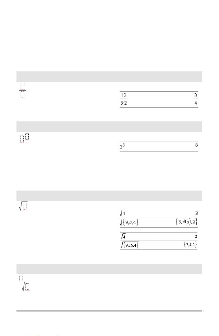
Fraction template
/p keys
Note: See also / (divide), page 175.
Example:
Exponent template
l key
Note: Type the first value, press l, and
then type the exponent. To return the cursor
to the baseline, press right arrow (¢).
Note: See also ^ (power), page 176.
Example:
Square root template
/q keys
Note: See also √() (square root), page
185.
Example:
Nth root template
/l keys
Note: See also root(), page 129.
Example:
Expression Templates 1
2 Expression Templates
Nth root template
/l keys
e exponent template
u keys
Natural exponential e raised to a power
Note: See also e^(), page 43.
Example:
Log template
/s key
Calculates log to a specified base. For a
default of base 10, omit the base.
Note: See also log(), page 86.
Example:
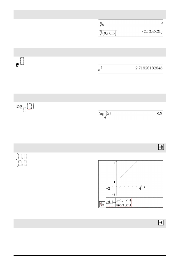
Piecewise template (2-piece)
Catalog >
Lets you create expressions and conditions
for a two-piece piecewise function. To add
a piece, click in the template and repeat the
template.
Note: See also piecewise(), page 110.
Example:
Piecewise template (N-piece)
Catalog >
Lets you create expressions and conditions
for an N-piece piecewise function. Prompts
for N.
Example:
See the example for Piecewise template (2-
piece).
Piecewise template (N-piece)
Catalog >
Note: See also piecewise(), page 110.
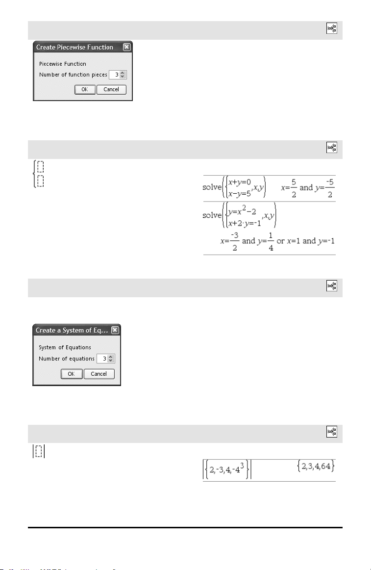
System of 2 equations template
Catalog >
Creates a system of two linear equations.
To add a row to an existing system, click in
the template and repeat the template.
Note: See also system(), page 150.
Example:
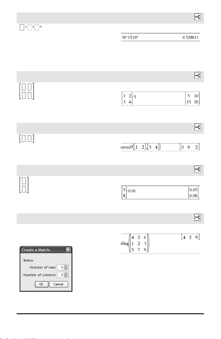
System of N equations template
Catalog >
Lets you create a system of N linear
equations. Prompts for N.
Note: See also system(), page 150.
Example:
See the example for System of equations
template (2-equation).
Absolute value template
Catalog >
Note: See also abs(), page 7.
Example:
Expression Templates 3
4 Expression Templates
dd°mm’ss.ss’’ template
Catalog >
Lets you enter angles in dd°mm’ss.ss’’
format, where dd is the number of decimal
degrees, mm is the number of minutes, and
ss.ss is the number of seconds.
Example:
Matrix template (2 x 2)
Catalog >
Creates a 2 x 2 matrix.
Example:
Matrix template (1 x 2)
Catalog >
.
Example:
Matrix template (2 x 1)
Catalog >
Example:
Matrix template (m x n)
Catalog >
The template appears after you are
prompted to specify the number of rows
and columns.
Example:
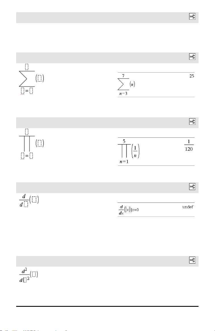
Matrix template (m x n)
Catalog >
Note: If you create a matrix with a large
number of rows and columns, it may take a
few moments to appear.
Sum template (Σ)
Catalog >
Note: See also Σ() (sumSeq), page 186.
Example:
Product template (Π)
Catalog >
Note: See also Π() (prodSeq), page 185.
Example:
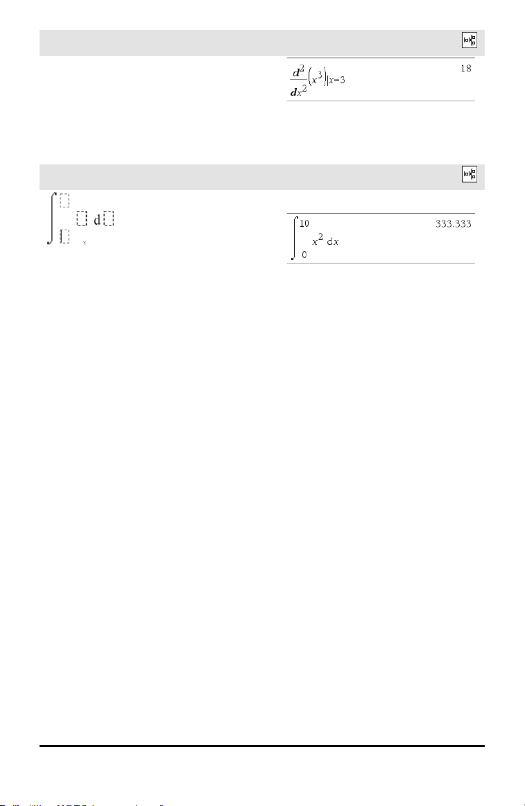
First derivative template
Catalog >
The first derivative template can be used to
calculate first derivative at a point
numerically, using auto differentiation
methods.
Note: See also d() (derivative), page 184.
Example:
Second derivative template
Catalog >
Example:
Expression Templates 5
6 Expression Templates
Second derivative template
Catalog >
The second derivative template can be used
to calculate second derivative at a point
numerically, using auto differentiation
methods.
Note: See also d() (derivative), page 184.
Definite integral template
Catalog >
The definite integral template can be used
to calculate the definite integral
numerically, using the same method as nInt
().
Note: See also nInt(), page 101.
Example:
Alphabetical Listing
Items whose names are not alphabetic (such as +, !, and >) are listed at the end of this
section, page 173. Unless otherwise specified, all examples in this section were
performed in the default reset mode, and all variables are assumed to be undefined.
A
abs()
Catalog >
abs(Value1) ⇒ value
abs(List1) ⇒ list
abs(Matrix1) ⇒ matrix
Returns the absolute value of the
argument.
Note: See also Absolute value template,
page 3.
If the argument is a complex number,
returns the number’s modulus.
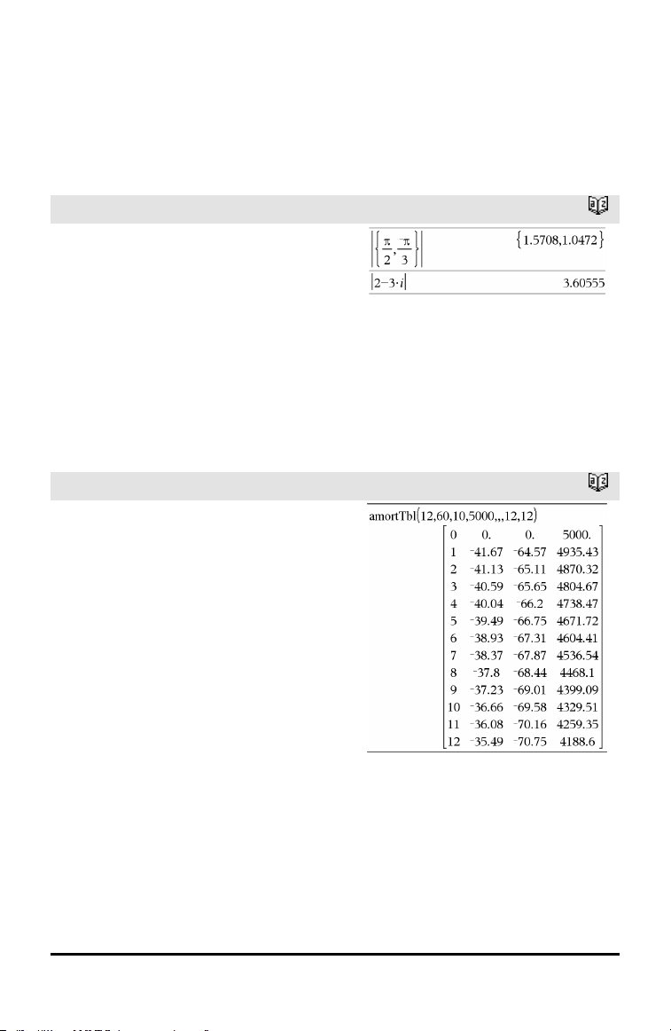
amortTbl()
Catalog >
amortTbl(NPmt,N,I,PV, [Pmt], [FV],
[PpY], [CpY], [PmtAt], [roundValue]) ⇒
matrix
Amortization function that returns a matrix
as an amortization table for a set of TVM
arguments.
NPmt is the number of payments to be
included in the table. The table starts with
the first payment.
N, I, PV, Pmt, FV, PpY, CpY, and PmtAt
are described in the table of TVM
arguments, page 161.
• If you omit Pmt, it defaults to
Pmt=tvmPmt
(N,I,PV,FV,PpY,CpY,PmtAt).
• If you omit FV, it defaults to FV=0.
• The defaults for PpY, CpY, and PmtAt
are the same as for the TVM functions.
roundValue specifies the number of
decimal places for rounding. Default=2.
Alphabetical Listing 7
8 Alphabetical Listing
amortTbl()
Catalog >
The columns in the result matrix are in this
order: Payment number, amount paid to
interest, amount paid to principal, and
balance.
The balance displayed in row n is the
balance after payment n.
You can use the output matrix as input for
the other amortization functions ΣInt() and
ΣPrn(), page 186, and bal(), page 15.
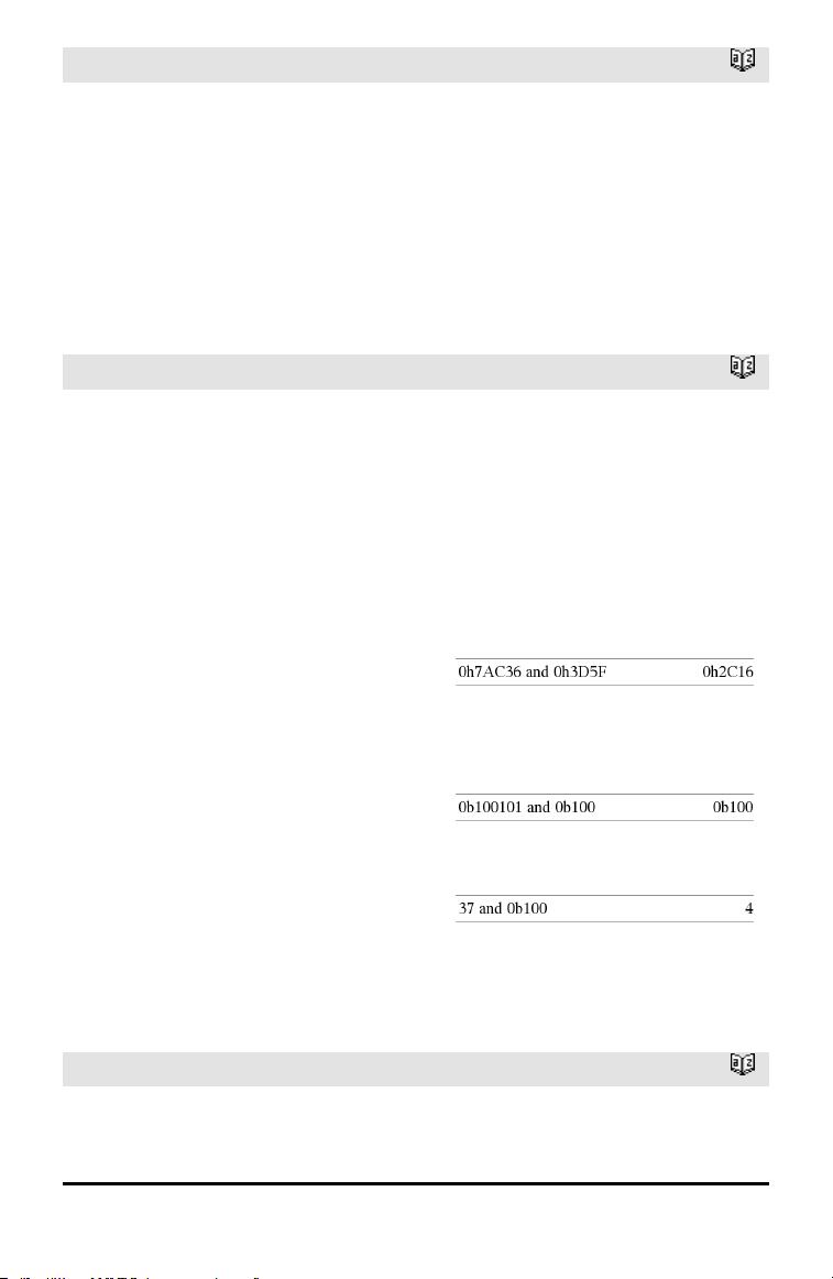
and
Catalog >
BooleanExpr1 and BooleanExpr2 ⇒
Boolean expression
BooleanList1 and BooleanList2 ⇒
Boolean list
BooleanMatrix1 and BooleanMatrix2 ⇒
Boolean matrix
Returns true or false or a simplified form of
the original entry.
Integer1 andInteger2 ⇒ integer
Compares two real integers bit-by-bit using
an and operation. Internally, both integers
are converted to signed, 64-bit binary
numbers. When corresponding bits are
compared, the result is 1 if both bits are 1;
otherwise, the result is 0. The returned
value represents the bit results, and is
displayed according to the Base mode.
You can enter the integers in any number
base. For a binary or hexadecimal entry, you
must use the 0b or 0h prefix, respectively.
Without a prefix, integers are treated as
decimal (base10).
In Hex base mode:
Important: Zero, not the letter O.
In Bin base mode:
In Dec base mode:
Note: A binary entry can have up to 64 digits
(not counting the 0b prefix). A hexadecimal
entry can have upto 16 digits.
angle()
Catalog >
angle(Value1) ⇒ value
In Degree angle mode:
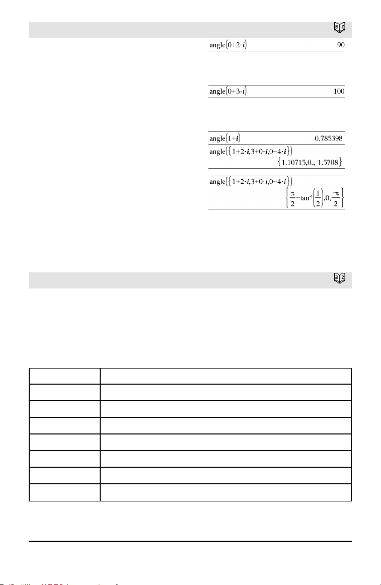
angle()
Catalog >
Returns the angle of the argument,
interpreting the argument as a complex
number.
In Gradian angle mode:
In Radian angle mode:
angle(List1) ⇒ list
angle(Matrix1) ⇒ matrix
Returns a list or matrix of angles of the
elements in List1 or Matrix1, interpreting
each element as a complex number that
represents a two-dimensional rectangular
coordinate point.
ANOVA
Catalog >
ANOVA List1,List2[,List3,...,List20][,Flag]
Performs a one-way analysis of variance for
comparing the means of two to 20
populations. A summary of results is stored
in the stat.results variable. (page 145)
Flag=0 for Data, Flag=1 for Stats
Output variable Description
stat.F Value of the F statistic
stat.PVal Smallest level of significance at whichthe null hypothesis can be rejected
stat.df Degrees of freedom of the groups
stat.SS Sum of squares of the groups
stat.MS Mean squares for the groups
stat.dfError Degrees of freedom of the errors
stat.SSError Sum of squares of the errors
Alphabetical Listing 9

10 Alphabetical Listing
Output variable Description
stat.MSError Mean square for the errors
stat.sp Pooled standard deviation
stat.xbarlist Mean of the input of the lists
stat.CLowerList 95% confidence intervals for the mean of each input list
stat.CUpperList 95% confidence intervals for the mean of each input list
ANOVA2way
Catalog >
ANOVA2way List1,List2[,List3,…,List10]
[,levRow]
Computes a two-way analysis of variance for
comparing the means of two to 10
populations. A summary of results is stored
in the stat.results variable. (See page 145.)
LevRow=0 for Block
LevRow=2,3,...,Len-1, for Two Factor,
where Len=length(List1)=length(List2) = …
= length(List10) and Len/LevRow Î
{2,3,…}
Outputs: Block Design
Output variable Description
stat.F Fstatistic of the column factor
stat.PVal Smallest level of significance at whichthe null hypothesis can be rejected
stat.df Degrees of freedom of the column factor
stat.SS Sum of squares of the column factor
stat.MS Mean squares for column factor
stat.FBlock F statistic for factor
stat.PValBlock Least probability at which the null hypothesis can be rejected
stat.dfBlock Degrees of freedom for factor
stat.SSBlock Sum of squares for factor
stat.MSBlock Meansquares for factor
stat.dfError Degrees of freedom of the errors

Output variable Description
stat.SSError Sum of squares of the errors
stat.MSError Mean squares for the errors
stat.s Standard deviation of the error
COLUMN FACTOR Outputs
Output variable Description
stat.Fcol F statistic of the column factor
stat.PValCol Probability value of the column factor
stat.dfCol Degrees of freedom of the column factor
stat.SSCol Sum of squares of the column factor
stat.MSCol Mean squares for column factor
ROW FACTOR Outputs
Output variable Description
stat.FRow F statisticof the row factor
stat.PValRow Probability value of the row factor
stat.dfRow Degrees of freedom of the row factor
stat.SSRow Sum of squares of the row factor
stat.MSRow Mean squares for row factor
INTERACTION Outputs
Output variable Description
stat.FInteract F statistic of the interaction
stat.PValInteract Probability value of the interaction
stat.dfInteract Degrees of freedom of the interaction
stat.SSInteract Sum of squares of the interaction
stat.MSInteract Mean squares for interaction
ERROR Outputs
Alphabetical Listing 11
12 Alphabetical Listing
Output variable Description
stat.dfError Degrees of freedom of the errors
stat.SSError Sum of squares of the errors
stat.MSError Mean squares for the errors
s Standard deviation of the error
Ans
/v keys
Ans ⇒ value
Returns the result of the most recently
evaluated expression.
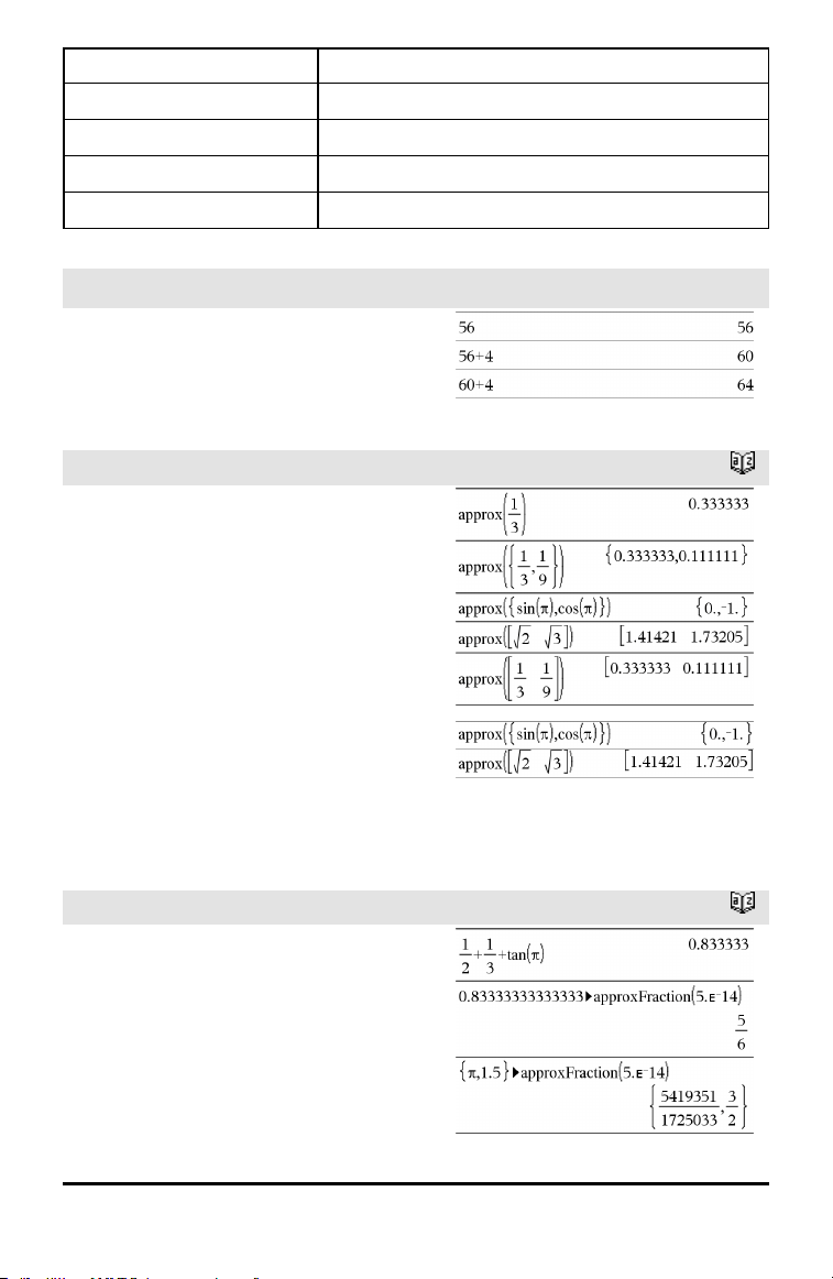
approx()
Catalog >
approx(Value1) ⇒ number
Returns the evaluation of the argument as
an expression containing decimal values,
when possible, regardless of the current
Auto or Approximate mode.
This is equivalent to entering the argument
and pressing /·.
approx(List1) ⇒ list
approx(Matrix1) ⇒ matrix
Returns a list or matrix where each
element has been evaluated to a decimal
value, when possible.
►approxFraction()
Catalog >
Value►approxFraction([Tol]) ⇒ value
List►approxFraction([Tol]) ⇒ list
Matrix►approxFraction([Tol]) ⇒ matrix
Returns the input as a fraction, using a
tolerance of Tol. If Tol is omitted, a
tolerance of 5.E-14 is used.

►approxFraction()
Catalog >
Note: You can insert this function from the
computer keyboard by typing
@>approxFraction(...).
approxRational()
Catalog >
approxRational(Value[, Tol]) ⇒ value
approxRational(List[, Tol]) ⇒ list
approxRational(Matrix[, Tol]) ⇒ matrix
Returns the argument as a fraction using a
tolerance of Tol. If Tol is omitted, a
tolerance of 5.E-14 is used.
arccos()
See cos⁻¹(), page 26.
arccosh()
See cosh⁻¹(), page 27.
arccot()
See cot⁻¹(), page 28.
arccoth()
See coth⁻¹(), page 29.
arccsc()
See csc⁻¹(), page 31.
arccsch()
See csch⁻¹(), page 32.
Alphabetical Listing 13
14 Alphabetical Listing
arcsec()
See sec⁻¹(), page 133.
arcsech()
See sech⁻¹(), page 133.
arcsin()
See sin⁻¹(), page 141.
arcsinh()
See sinh⁻¹(), page 142.
arctan()
See tan⁻¹(), page 152.
arctanh()
See tanh⁻¹(), page 153.
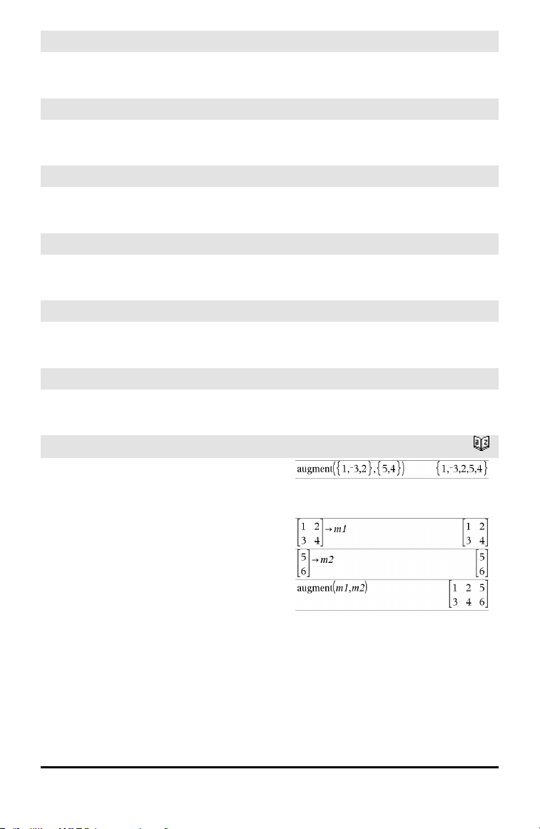
augment()
Catalog >
augment(List1, List2) ⇒ list
Returns a new list that is List2 appended to
the end of List1.
augment(Matrix1, Matrix2) ⇒ matrix
Returns a new matrix that is Matrix2
appended to Matrix1. When the “,”
character is used, the matrices must have
equal row dimensions, and Matrix2 is
appended to Matrix1 as new columns.
Does not alter Matrix1 or Matrix2.
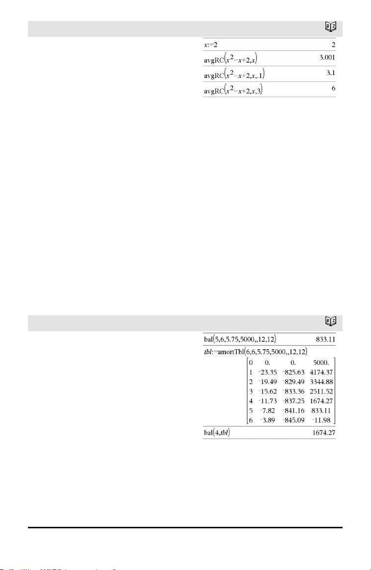
avgRC()
Catalog >
avgRC(Expr1, Var [=Value] [, Step]) ⇒
expression
avgRC(Expr1, Var [=Value] [, List1]) ⇒
list
avgRC(List1, Var [=Value] [, Step]) ⇒
list
avgRC(Matrix1, Var [=Value] [, Step]) ⇒
matrix
Returns the forward-difference quotient
(average rate of change).
Expr1 can be a user-defined function name
(see Func).
When Value is specified, it overrides any
prior variable assignment or any current “|”
substitution for the variable.
Step is the step value. If Step is omitted, it
defaults to 0.001.
Note that the similar function centralDiff()
uses the central-difference quotient.
B
bal()
Catalog >
bal(NPmt,N,I,PV ,[Pmt], [FV], [PpY],
[CpY], [PmtAt], [roundValue]) ⇒ value
bal(NPmt,amortTable) ⇒ value
Amortization function that calculates
schedule balance after a specified payment.
N, I, PV, Pmt, FV, PpY, CpY, and PmtAt
are described in the table of TVM
arguments, page 161.
NPmt specifies the payment number after
which you want the data calculated.
N, I, PV, Pmt, FV, PpY, CpY, and PmtAt
are described in the table of TVM
arguments, page 161.
Alphabetical Listing 15
16 Alphabetical Listing
bal()
Catalog >
• If you omit Pmt, it defaults to
Pmt=tvmPmt
(N,I,PV,FV,PpY,CpY,PmtAt).
• If you omit FV, it defaults to FV=0.
• The defaults for PpY, CpY, and PmtAt
are the same as for the TVM functions.
roundValue specifies the number of
decimal places for rounding. Default=2.
bal(NPmt,amortTable) calculates the
balance after payment number NPmt,
based on amortization table amortTable.
The amortTable argument must be a
matrix in the form described under
amortTbl(), page 7.
Note: See also ΣInt() and ΣPrn(), page 186.
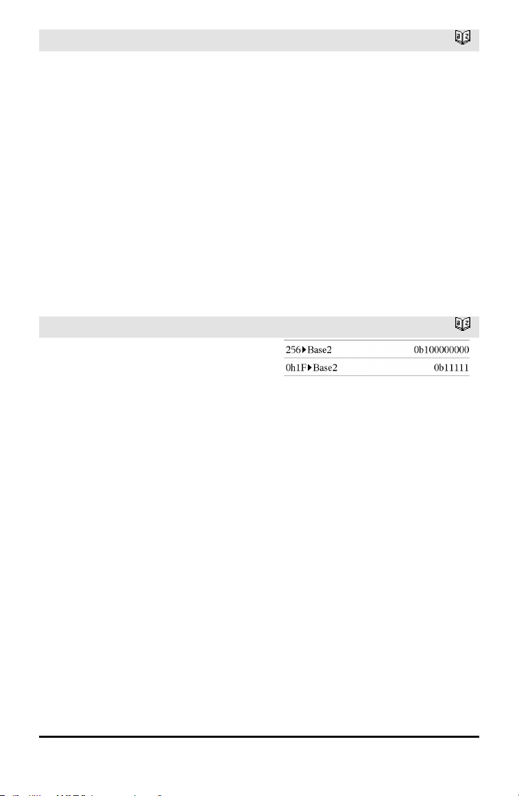
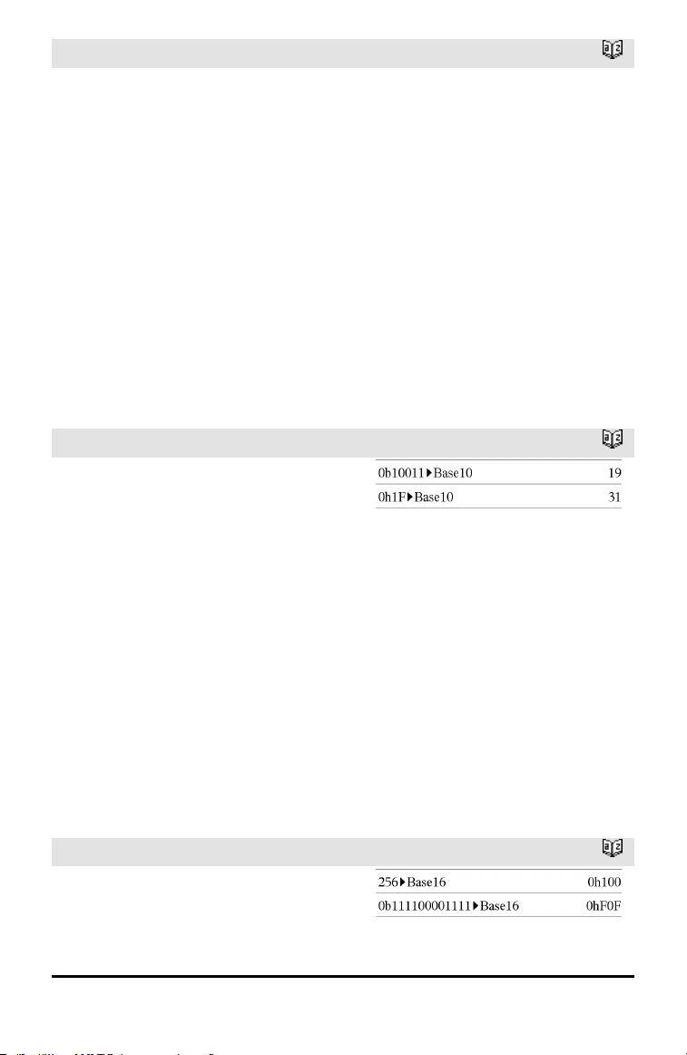
►Base2
Catalog >
Integer1 ►Base2 ⇒ integer
Note: You can insert this operator from the
computer keyboard by typing @>Base2.
Converts Integer1 to a binary number.
Binary or hexadecimal numbers always
have a 0b or 0h prefix, respectively. Use a
zero, not the letter O, followed by b or h.
0b binaryNumber
0h hexadecimalNumber
A binary number can have up to 64 digits. A
hexadecimal number can have up to 16.
Without a prefix, Integer1 is treated as
decimal (base10). The result is displayed in
binary, regardless of the Base mode.
Negative numbers are displayed in “two's
complement” form. For example,
⁻1is displayed as
0hFFFFFFFFFFFFFFFFin Hex base mode
0b111...111 (641’s)in Binary base mode
⁻2
63
is displayed as
0h8000000000000000in Hex base mode
0b100...000 (63 zeros)in Binary base mode
►Base2
Catalog >
If you enter a decimal integer that is
outside the range of a signed, 64-bit binary
form, a symmetric modulo operation is
used to bring the value into the appropriate
range. Consider the following examples of
values outside the range.
2
63
becomes ⁻2
63
and is displayed as
0h8000000000000000in Hex base mode
0b100...000 (63 zeros)in Binary base mode
2
64
becomes 0 and is displayed as
0h0in Hex base mode
0b0in Binary base mode
⁻2
63
− 1 becomes 2
63
− 1 and is displayed
as
0h7FFFFFFFFFFFFFFFin Hex base mode
0b111...111 (641’s)in Binary base mode
►Base10
Catalog >
Integer1 ►Base10 ⇒ integer
Note: You can insert this operator from the
computer keyboard by typing @>Base10.
Converts Integer1 to a decimal (base10)
number. A binary or hexadecimal entry
must always have a 0b or 0h prefix,
respectively.
0b binaryNumber
0h hexadecimalNumber
Zero, not the letter O, followed by b or h.
A binary number can have up to 64 digits. A
hexadecimal number can have up to 16.
Without a prefix, Integer1 is treated as
decimal. The result is displayed in decimal,
regardless of the Base mode.
►Base16
Catalog >
Integer1 ►Base16 ⇒ integer
Note: You can insert this operator from the
computer keyboard by typing @>Base16.
Alphabetical Listing 17

18 Alphabetical Listing
►Base16
Catalog >
Converts Integer1 to a hexadecimal
number. Binary or hexadecimal numbers
always have a 0b or 0h prefix, respectively.
0b binaryNumber
0h hexadecimalNumber
Zero, not the letter O, followed by b or h.
A binary number can have up to 64 digits. A
hexadecimal number can have up to 16.
Without a prefix, Integer1 is treated as
decimal (base10). The result is displayed in
hexadecimal, regardless of the Base mode.
If you enter a decimal integer that is too
large for a signed, 64-bit binary form, a
symmetric modulo operation is used to
bring the value into the appropriate range.
For more information, see ►Base2, page
16.
binomCdf()
Catalog >
binomCdf(n,p) ⇒ list
binomCdf(n,p,lowBound,upBound) ⇒
number if lowBound and upBound are
numbers, list if lowBound and upBound are
lists
binomCdf(n,p,upBound)for P(0≤X≤upBound)
⇒ number if upBound is a number, list if
upBound is a list
Computes a cumulative probability for the
discrete binomial distribution with n number
of trials and probability p of success on each
trial.
For P(X ≤ upBound), set lowBound=0
binomPdf()
Catalog >
binomPdf(n,p) ⇒ list
binomPdf(n,p,XVal) ⇒ number if XVal is a
number, list if XVal is a list
binomPdf()
Catalog >
Computes a probability for the discrete
binomial distribution with n number of trials
and probability p of success on each trial.
C
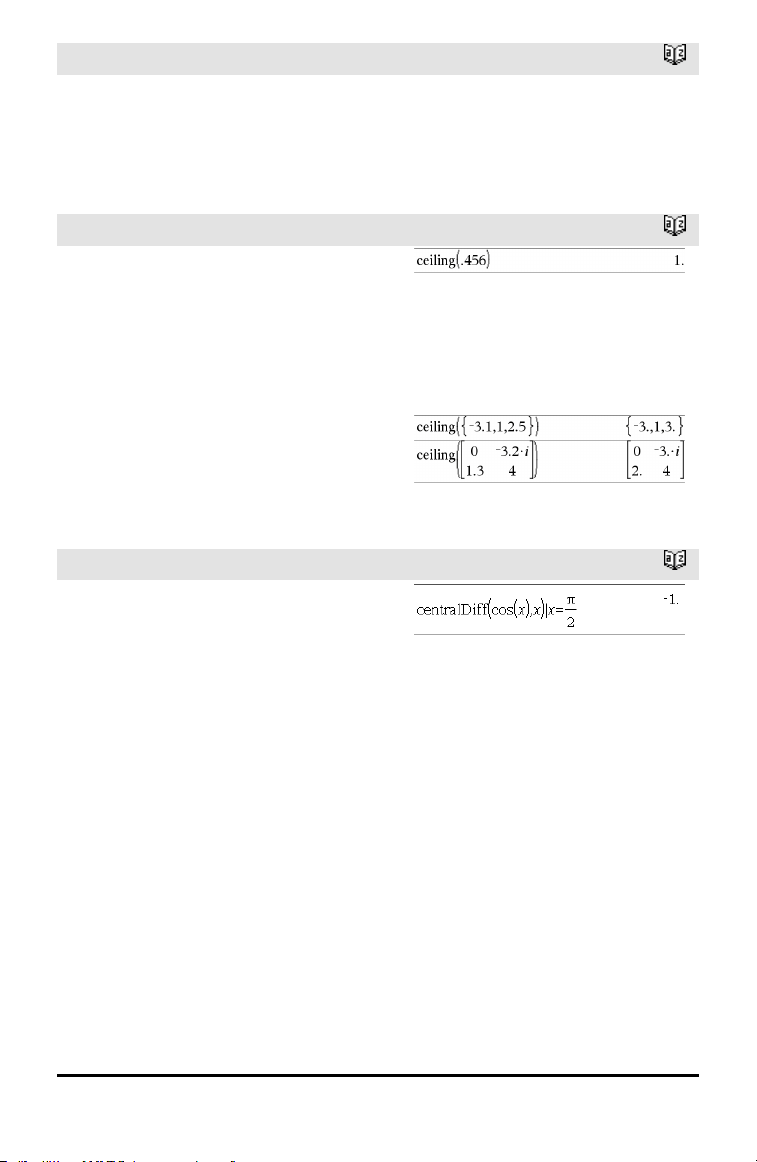
Catalog >
ceiling(Value1) ⇒ value
Returns the nearest integer that is ≥ the
argument.
The argument can be a real or a complex
number.
Note: See also floor().
ceiling(List1) ⇒ list
ceiling(Matrix1) ⇒ matrix
Returns a list or matrix of the ceiling of
each element.
centralDiff()
Catalog >
centralDiff(Expr1,Var [=Value][,Step]) ⇒
expression
centralDiff(Expr1,Var [,Step])|Var=Value
⇒ expression
centralDiff(Expr1,Var [=Value][,List]) ⇒
list
centralDiff(List1,Var [=Value][,Step]) ⇒
list
centralDiff(Matrix1,Var [=Value][,Step])
⇒ matrix
Returns the numerical derivative using the
central difference quotient formula.
When Value is specified, it overrides any
prior variable assignment or any current “|”
substitution for the variable.
Step is the step value. If Step is omitted, it
defaults to 0.001.
Alphabetical Listing 19

20 Alphabetical Listing
centralDiff()
Catalog >
When using List1 or Matrix1, the operation
gets mapped across the values in the list or
across the matrix elements.
Note: See also avgRC().
char()
Catalog >
char(Integer) ⇒ character
Returns a character string containing the
character numbered Integer from the
handheld character set. The valid range for
Integer is 0–65535.
χ
2
2way
Catalog >
χ
2
2way obsMatrix
chi22way obsMatrix
Computes a χ
2
test for association on the
two-way table of counts in the observed
matrix obsMatrix. A summary of results is
stored in the stat.results variable. (page
145)
For information on the effect of empty
elements in a matrix, see “Empty (Void)
Elements,” page 196.
Output variable Description
stat.χ
2
Chi square stat: sum (observed - expected)
2
/expected
stat.PVal Smallest level of significance at whichthe null hypothesis can be rejected
stat.df Degrees of freedom for the chi square statistics
stat.ExpMat Matrix of expected elemental count table, assuming null hypothesis
stat.CompMat Matrix of elemental chi square statistic contributions
χ
2
Cdf()
Catalog >
χ
2
Cdf(lowBound,upBound,df) ⇒ number if
lowBound and upBound are numbers, list if
lowBound and upBound are lists

χ
2
Cdf()
Catalog >
chi2Cdf(lowBound,upBound,df) ⇒ number
if lowBound and upBound are numbers, list
if lowBound and upBound are lists
Computes the χ
2
distribution probability
between lowBound and upBound for the
specified degrees of freedom df.
For P(X ≤ upBound), set lowBound = 0.
For information on the effect of empty
elements in a list, see “Empty (Void)
Elements,” page 196.
χ
2
GOF
Catalog >
χ
2
GOF obsList,expList,df
chi2GOF obsList,expList,df
Performs a test to confirm that sample data
is from a population that conforms to a
specified distribution. obsList is a list of
counts and must contain integers. A
summary of results is stored in the
stat.results variable. (See page 145.)
For information on the effect of empty
elements in a list, see “Empty (Void)
Elements,” page 196.
Output variable Description
stat.χ
2
Chi square stat: sum((observed - expected)
2
/expected
stat.PVal Smallest level of significance at whichthe null hypothesis can be rejected
stat.df Degrees of freedom for the chi square statistics
stat.CompList Elemental chi square statisticcontributions
χ
2
Pdf()
Catalog >
χ
2
Pdf(XVal,df) ⇒ number if XVal is a
number, list if XVal is a list
chi2Pdf(XVal,df) ⇒ number if XVal is a
number, list if XVal is a list
Alphabetical Listing 21

22 Alphabetical Listing
χ
2
Pdf()
Catalog >
Computes the probability density function
(pdf) for the χ
2
distribution at a specified
XVal value for the specified degrees of
freedom df.
For information on the effect of empty
elements in a list, see “Empty (Void)
Elements,” page 196.
ClearAZ
Catalog >
ClearAZ
Clears all single-character variables in the
current problem space.
If one or more of the variables are locked,
this command displays an error message
and deletes only the unlocked variables. See
unLock, page 163.
ClrErr
Catalog >
ClrErr
Clears the error status and sets system
variable errCode to zero.
The Else clause of the Try...Else...EndTry
block should use ClrErr or PassErr. If the
error is to be processed or ignored, use
ClrErr. If what to do with the error is not
known, use PassErr to send it to the next
error handler. If there are no more pending
Try...Else...EndTry error handlers, the error
dialog box will be displayed as normal.
Note: See also PassErr, page 109, and Try,
page 157.
Note for entering the example: For
instructions on entering multi-line program
and function definitions, refer to the
Calculator section of your product guidebook.
For an example of ClrErr, See Example 2
under the Try command, page 157.
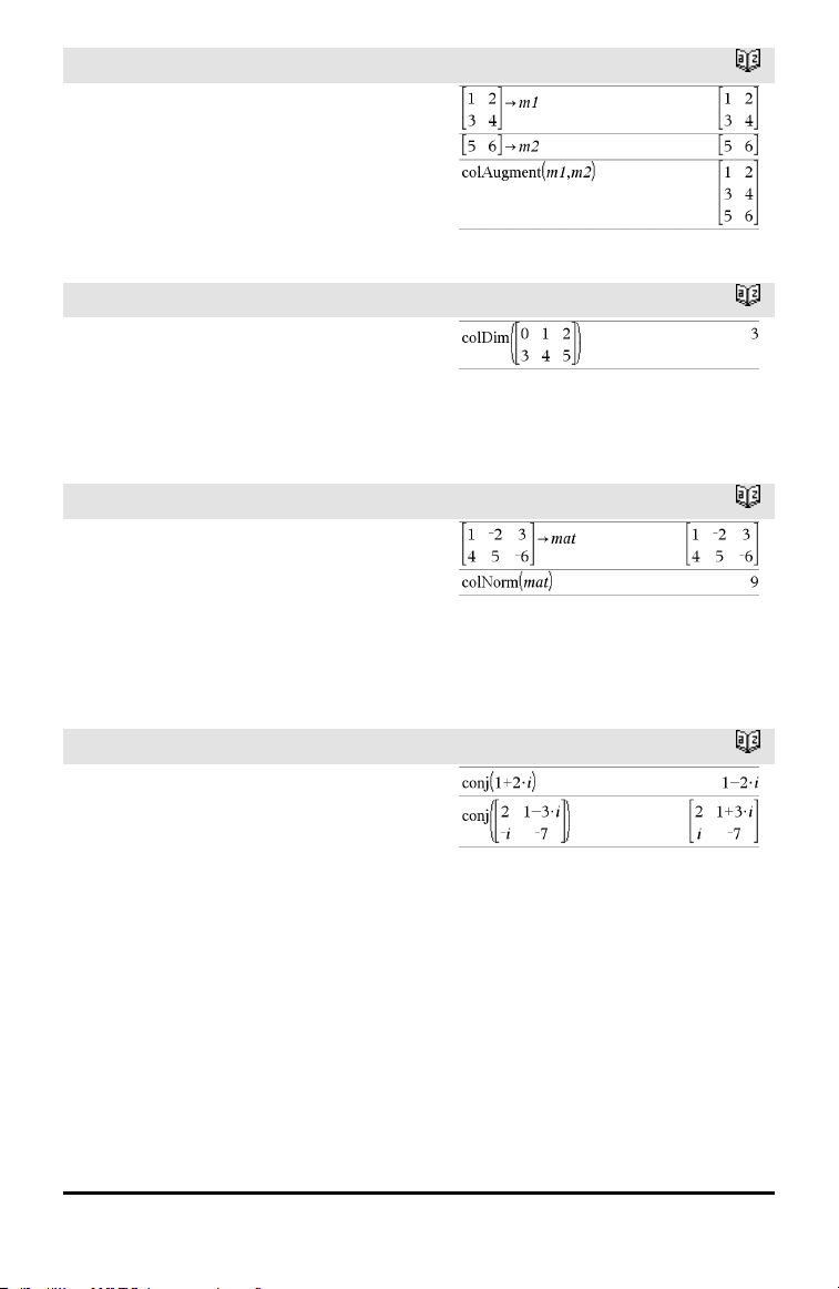
colAugment()
Catalog >
colAugment(Matrix1, Matrix2) ⇒ matrix
Returns a new matrix that is Matrix2
appended to Matrix1. The matrices must
have equal column dimensions, and
Matrix2 is appended to Matrix1 as new
rows. Does not alter Matrix1 or Matrix2.
colDim()
Catalog >
colDim(Matrix) ⇒ expression
Returns the number of columns contained
in Matrix.
Note: See also rowDim().
colNorm()
Catalog >
colNorm(Matrix) ⇒ expression
Returns the maximum of the sums of the
absolute values of the elements in the
columns in Matrix.
Note: Undefined matrix elements are not
allowed. See also rowNorm().
conj()
Catalog >
conj(Value1) ⇒ value
conj(List1) ⇒ list
conj(Matrix1) ⇒ matrix
Returns the complex conjugate of the
argument.
Alphabetical Listing 23
24 Alphabetical Listing
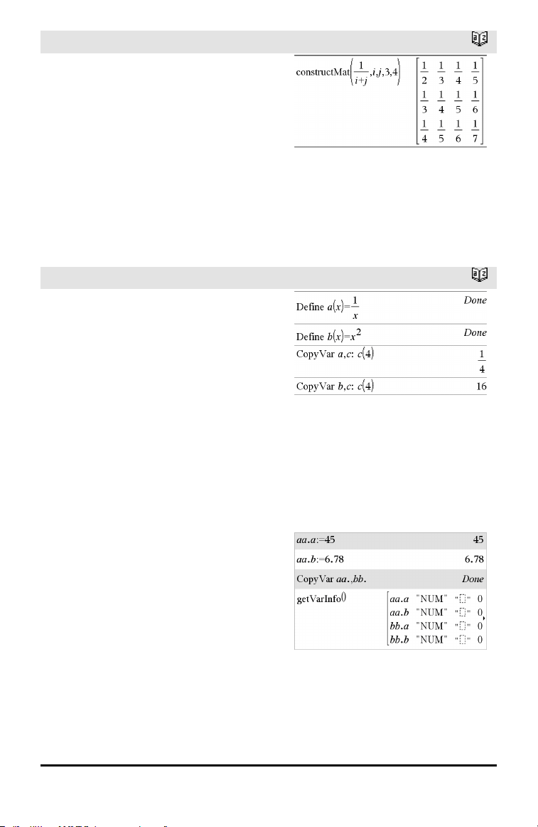
constructMat()
Catalog >
constructMat
(Expr,Var1,Var2,numRows,numCols) ⇒
matrix
Returns a matrix based on the arguments.
Expr is an expression in variables Var1 and
Var2. Elements in the resulting matrix are
formed by evaluating Expr for each
incremented value of Var1 and Var2.
Var1 is automatically incremented from 1
through numRows. Within each row, Var2
is incremented from 1 through numCols.
CopyVar
Catalog >
CopyVar Var1, Var2
CopyVar Var1., Var2.
CopyVar Var1, Var2 copies the value of
variable Var1 to variable Var2, creating
Var2 if necessary. Variable Var1 must have
a value.
If Var1 is the name of an existing user-
defined function, copies the definition of
that function to function Var2. Function
Var1 must be defined.
Var1 must meet the variable-naming
requirements or must be an indirection
expression that simplifies to a variable
name meeting the requirements.
CopyVar Var1., Var2. copies all members
of the Var1. variable group to the Var2.
group, creating Var2. if necessary.
Var1. must be the name of an existing
variable group, such as the statistics stat.nn
results, or variables created using the
LibShortcut() function. If Var2. already
exists, this command replaces all members
that are common to both groups and adds
the members that do not already exist. If
one or more members of Var2. are locked,
all members of Var2. are left unchanged.
corrMat()
Catalog >
corrMat(List1,List2[,…[,List20]])
Computes the correlation matrix for the
augmented matrix [List1, List2, ..., List20].
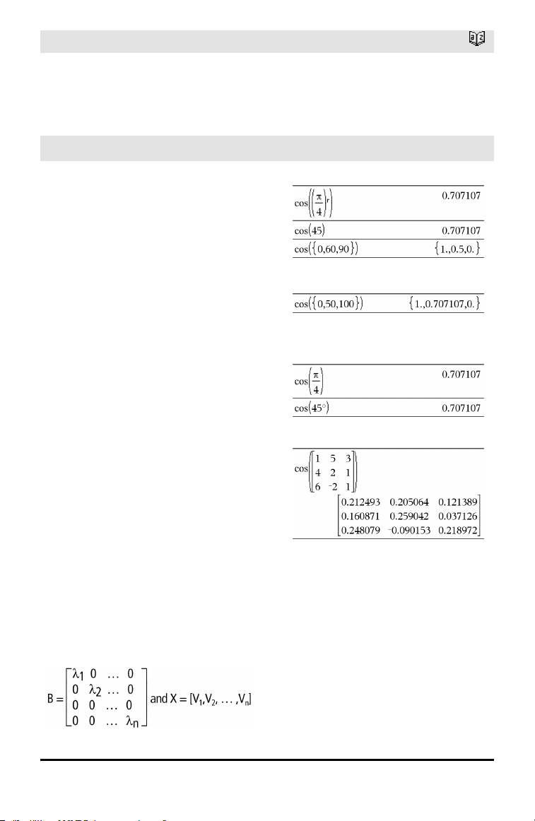
cos()
µ key
cos(Value1) ⇒ value
cos(List1) ⇒ list
cos(Value1) returns the cosine of the
argument as a value.
cos(List1) returns a list of the cosines of all
elements in List1.
Note: The argument is interpreted as a
degree, gradian or radian angle, according
to the current angle mode setting. You can
use °,
G
, or
r
to override the angle mode
temporarily.
In Degree angle mode:
In Gradian angle mode:
In Radian angle mode:
cos(squareMatrix1) ⇒ squareMatrix
Returns the matrix cosine of
squareMatrix1. This is not the same as
calculating the cosine of each element.
When a scalar function f(A) operates on
squareMatrix1 (A), the result is calculated
by the algorithm:
Compute the eigenvalues (λ
i
) and
eigenvectors (V
i
) of A.
squareMatrix1 must be diagonalizable.
Also, it cannot have symbolic variables that
have not been assigned a value.
Form the matrices:
In Radian angle mode:
Alphabetical Listing 25
26 Alphabetical Listing
cos()
µ key
Then A = X B X⁻¹ and f(A) = X f(B) X⁻¹. For
example, cos(A) = X cos(B) X⁻¹ where:
cos(B) =
All computations are performed using
floating-point arithmetic.
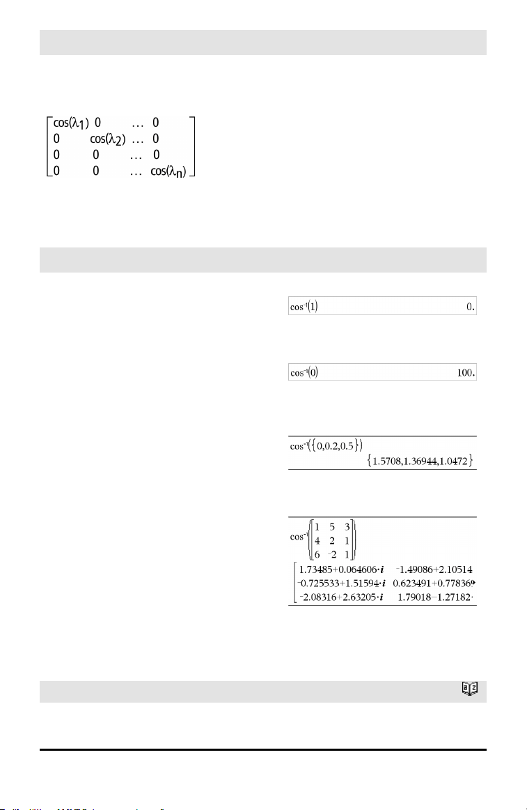
cos⁻¹()
µ key
cos⁻¹(Value1) ⇒ value
cos⁻¹(List1) ⇒ list
cos⁻¹(Value1) returns the angle whose
cosine is Value1.
cos⁻¹(List1) returns a list of the inverse
cosines of each element of List1.
Note: The result is returned as a degree,
gradian or radian angle, according to the
current angle mode setting.
Note: You can insert this function from the
keyboard by typing arccos(...).
In Degree angle mode:
In Gradian angle mode:
In Radian angle mode:
cos⁻¹(squareMatrix1) ⇒ squareMatrix
Returns the matrix inverse cosine of
squareMatrix1. This is not the same as
calculating the inverse cosine of each
element. For information about the
calculation method, refer to cos().
squareMatrix1 must be diagonalizable. The
result always contains floating-point
numbers.
In Radian angle mode and Rectangular
Complex Format:
To see the entire result, press £ and then
use ¡and¢ to move the cursor.
cosh()
Catalog >
In Degree angle mode:
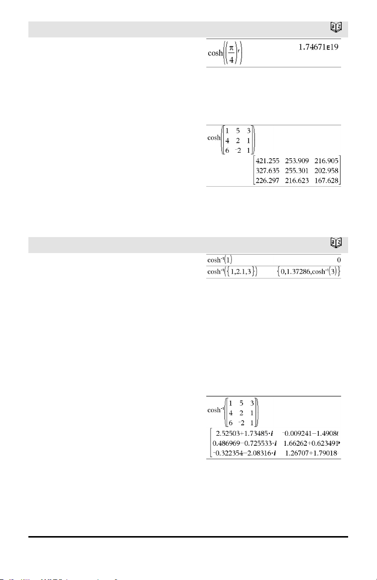
cosh()
Catalog >
cosh(Value1) ⇒ value
cosh(List1) ⇒ list
cosh(Value1) returns the hyperbolic cosine
of the argument.
cosh(List1) returns a list of the hyperbolic
cosines of each element of List1.
cosh(squareMatrix1) ⇒ squareMatrix
Returns the matrix hyperbolic cosine of
squareMatrix1. This is not the same as
calculating the hyperbolic cosine of each
element. For information about the
calculation method, refer to cos().
squareMatrix1 must be diagonalizable. The
result always contains floating-point
numbers.
In Radian angle mode:
cosh⁻¹()
Catalog >
cosh⁻¹(Value1) ⇒ value
cosh⁻¹(List1) ⇒ list
cosh⁻¹(Value1) returns the inverse
hyperbolic cosine of the argument.
cosh⁻¹(List1) returns a list of the inverse
hyperbolic cosines of each element of
List1.
Note: You can insert this function from the
keyboard by typing arccosh(...).
cosh⁻¹(squareMatrix1) ⇒ squareMatrix
Returns the matrix inverse hyperbolic
cosine of squareMatrix1. This is not the
same as calculating the inverse hyperbolic
cosine of each element. For information
about the calculation method, refer to cos
().
squareMatrix1 must be diagonalizable. The
result always contains floating-point
numbers.
In Radian angle mode and In Rectangular
Complex Format:
To see the entire result, press £ and then
use ¡and¢ to move the cursor.
Alphabetical Listing 27
28 Alphabetical Listing
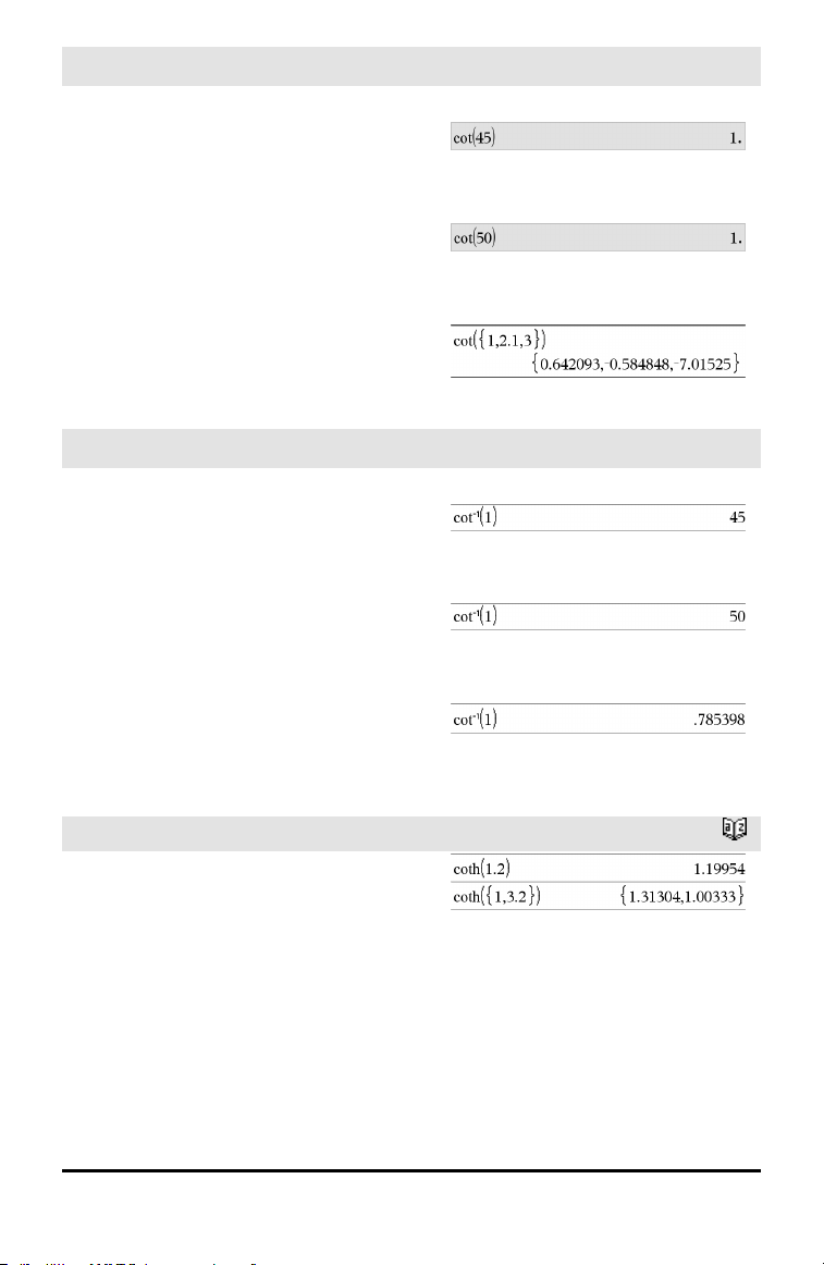
cot()
µ key
cot(Value1) ⇒ value
cot(List1) ⇒ list
Returns the cotangent of Value1 or returns
a list of the cotangents of all elements in
List1.
Note: The argument is interpreted as a
degree, gradian or radian angle, according
to the current angle mode setting. You can
use °,
G
, or
r
to override the angle mode
temporarily.
In Degree angle mode:
In Gradian angle mode:
In Radian angle mode:
cot⁻¹()
µ key
cot⁻¹(Value1) ⇒ value
cot⁻¹(List1) ⇒ list
Returns the angle whose cotangent is
Value1 or returns a list containing the
inverse cotangents of each element of
List1.
Note: The result is returned as a degree,
gradian or radian angle, according to the
current angle mode setting.
Note: You can insert this function from the
keyboard by typing arccot(...).
In Degree angle mode:
In Gradian angle mode:
In Radian angle mode:
coth()
Catalog >
coth(Value1) ⇒ value
coth(List1) ⇒ list
Returns the hyperbolic cotangent of Value1
or returns a list of the hyperbolic
cotangents of all elements of List1.
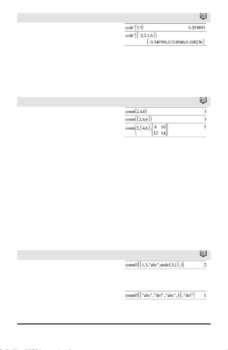
coth⁻¹()
Catalog >
coth⁻¹(Value1) ⇒ value
coth⁻¹(List1) ⇒ list
Returns the inverse hyperbolic cotangent of
Value1 or returns a list containing the
inverse hyperbolic cotangents of each
element of List1.
Note: You can insert this function from the
keyboard by typing arccoth(...).
count()
Catalog >
count(Value1orList1 [,Value2orList2
[,...]]) ⇒ value
Returns the accumulated count of all
elements in the arguments that evaluate to
numeric values.
Each argument can be an expression, value,
list, or matrix. You can mix data types and
use arguments of various dimensions.
For a list, matrix, or range of cells, each
element is evaluated to determine if it
should be included in the count.
Within the Lists & Spreadsheet application,
you can use a range of cells in place of any
argument.
Empty (void) elements are ignored. For
more information on empty elements, see
page 196.
countif()
Catalog >
countif(List,Criteria) ⇒ value
Returns the accumulated count of all
elements in List that meet the specified
Criteria.
Criteria can be:
• A value, expression, or string. For
Counts the number of elements equal to 3.
Alphabetical Listing 29
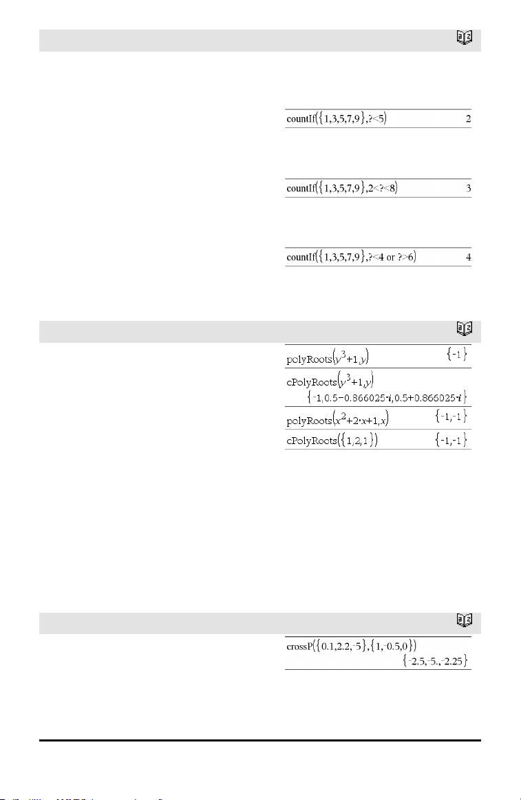
30 Alphabetical Listing
countif()
Catalog >
example, 3 counts only those elements in
List that simplify to the value 3.
• A Boolean expression containing the
symbol ? as a placeholder for each
element. For example, ?<5 counts only
those elements in List that are less than
5.
Within the Lists & Spreadsheet application,
you can use a range of cells in place of List.
Empty (void) elements in the list are
ignored. For more information on empty
elements, see page 196.
Note: See also sumIf(), page 149, and
frequency(), page 55.
Counts the number of elements equal to
“def.”
Counts 1 and 3.
Counts 3, 5, and 7.
Counts 1, 3, 7, and 9.
cPolyRoots()
Catalog >
cPolyRoots(Poly,Var) ⇒ list
cPolyRoots(ListOfCoeffs) ⇒ list
The first syntax, cPolyRoots(Poly,Var),
returns a list of complex roots of
polynomial Poly with respect to variable
Var.
Poly must be a polynomial in expanded
form in one variable. Do not use
unexpanded forms such as y
2
•y+1 or
x•x+2•x+1
The second syntax, cPolyRoots
(ListOfCoeffs), returns a list of complex
roots for the coefficients in ListOfCoeffs.
Note: See also polyRoots(), page 112.
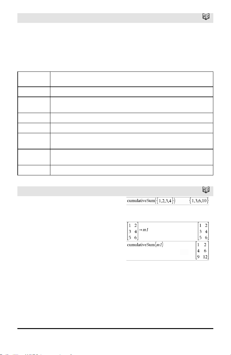
crossP()
Catalog >
crossP(List1, List2) ⇒ list
Returns the cross product of List1 and
List2 as a list.
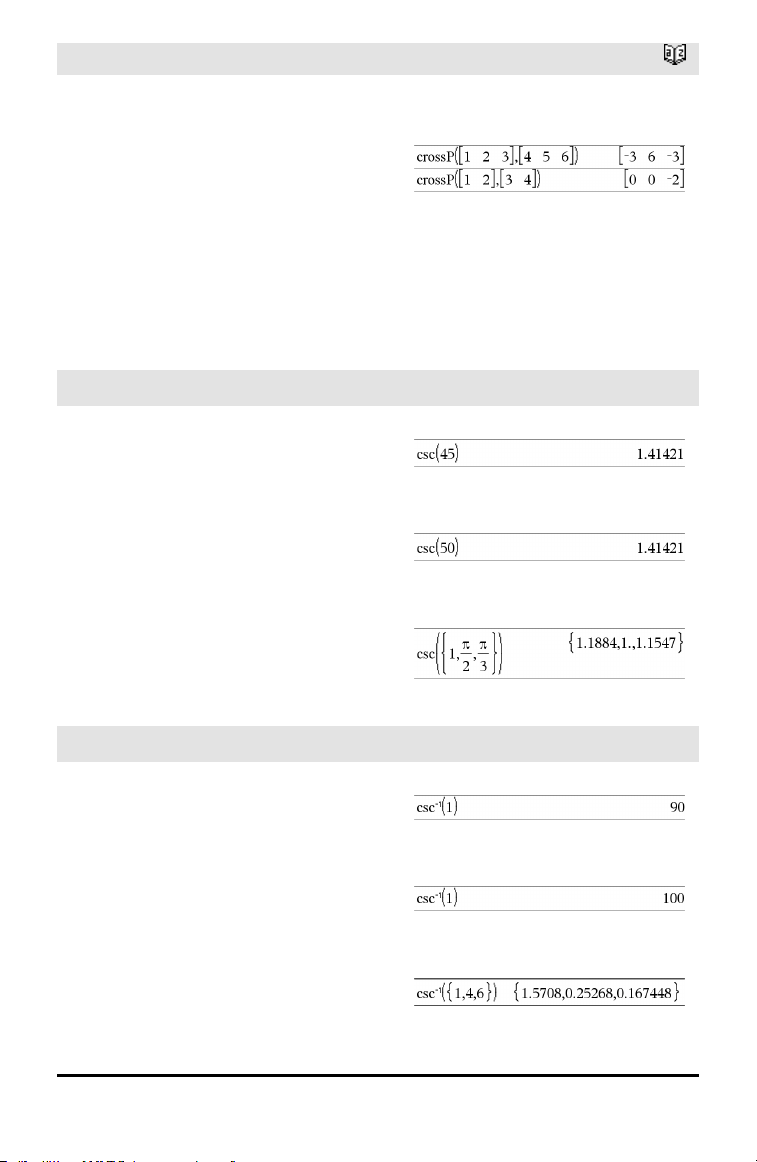
crossP()
Catalog >
List1 and List2 must have equal
dimension, and the dimension must be
either 2 or 3.
crossP(Vector1, Vector2) ⇒ vector
Returns a row or column vector (depending
on the arguments) that is the cross product
of Vector1 and Vector2.
Both Vector1 and Vector2 must be row
vectors, or both must be column vectors.
Both vectors must have equal dimension,
and the dimension must be either 2or3.
csc()
µ key
csc(Value1) ⇒ value
csc(List1) ⇒ list
Returns the cosecant of Value1 or returns a
list containing the cosecants of all elements
in List1.
In Degree angle mode:
In Gradian angle mode:
In Radian angle mode:
csc⁻¹()
µ key
csc⁻¹(Value1) ⇒ value
csc⁻¹(List1) ⇒ list
Returns the angle whose cosecant is
Value1 or returns a list containing the
inverse cosecants of each element of List1.
Note: The result is returned as a degree,
gradian or radian angle, according to the
current angle mode setting.
Note: You can insert this function from the
keyboard by typing arccsc(...).
In Degree angle mode:
In Gradian angle mode:
In Radian angle mode:
Alphabetical Listing 31

32 Alphabetical Listing
csch()
Catalog >
csch(Value1) ⇒ value
csch(List1) ⇒ list
Returns the hyperbolic cosecant of Value1
or returns a list of the hyperbolic cosecants
of all elements of List1.
csch⁻¹()
Catalog >
csch⁻¹(Value) ⇒ value
csch⁻¹(List1) ⇒ list
Returns the inverse hyperbolic cosecant of
Value1 or returns a list containing the
inverse hyperbolic cosecants of each
element of List1.
Note: You can insert this function from the
keyboard by typing arccsch(...).
CubicReg
Catalog >
CubicReg X, Y[, [Freq] [, Category,
Include]]
Computes the cubic polynomial regression
y=a•x
3
+b•x
2
+c•x+d on lists X and Y with
frequency Freq. A summary of results is
stored in the stat.results variable. (See page
145.)
All the lists must have equal dimension
except for Include.
X and Y are lists of independent and
dependent variables.
Freq is an optional list of frequency values.
Each element in Freq specifies the
frequency of occurrence for each
corresponding X and Y data point. The
default value is 1. All elements must be
integers ≥ 0.
Category is a list of numeric or string
category codes for the corresponding X and
Y data.
CubicReg
Catalog >
Include is a list of one or more of the
category codes. Only those data items
whose category code is included in this list
are included in the calculation.
For information on the effect of empty
elements in a list, see “Empty (Void)
Elements,” page 196.
Output
variable
Description
stat.RegEqn
Regression equation: a•x
3
+b•x
2
+c•x+d
stat.a, stat.b,
stat.c, stat.d
Regression coefficients
stat.R
2
Coefficientof determination
stat.Resid Residuals from the regression
stat.XReg
Listof data points in the modifiedX List actually used in the regression based on
restrictions of Freq, Category List, and Include Categories
stat.YReg
Listof data points in the modifiedY List actually used inthe regression basedon
restrictions of Freq, Category List, and Include Categories
stat.FreqReg
Listof frequencies corresponding to stat.XReg and stat.YReg
cumulativeSum()
Catalog >
cumulativeSum(List1) ⇒ list
Returns a list of the cumulative sums of the
elements in List1, starting at element1.
cumulativeSum(Matrix1) ⇒ matrix
Returns a matrix of the cumulative sums of
the elements in Matrix1. Each element is
the cumulative sum of the column from top
to bottom.
An empty (void) element in List1 or
Matrix1 produces a void element in the
resulting list or matrix. For more
information on empty elements, see page
196.
Alphabetical Listing 33
34 Alphabetical Listing
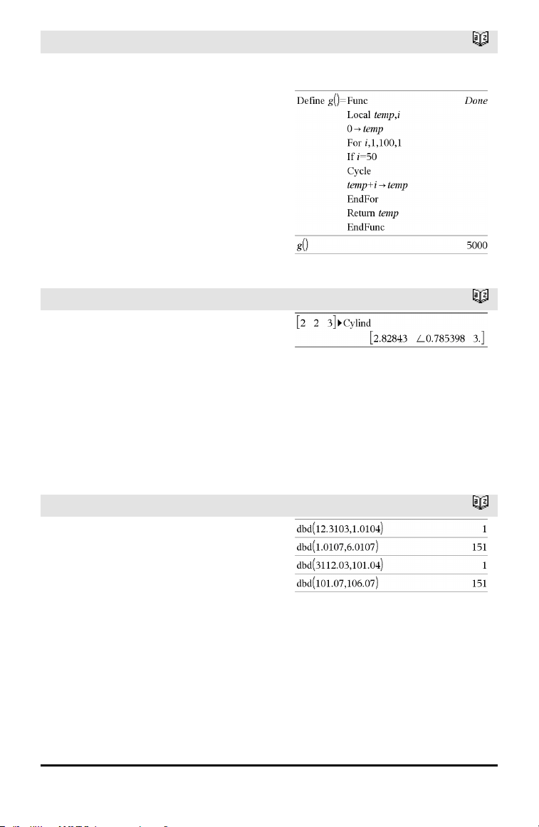
Cycle
Catalog >
Cycle
Transfers control immediately to the next
iteration of the current loop (For, While, or
Loop).
Cycle is not allowed outside the three
looping structures (For, While, or Loop).
Note for entering the example: For
instructions on entering multi-line program
and function definitions, refer to the
Calculator section of your product
guidebook.
Function listing that sums the integers from 1
to 100 skipping 50.
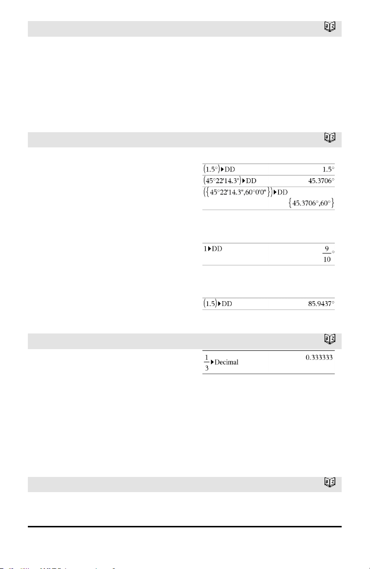
►Cylind
Catalog >
Vector ►Cylind
Note: You can insert this operator from the
computer keyboard by typing @>Cylind.
Displays the row or column vector in
cylindrical form [r,∠ θ, z].
Vector must have exactly three elements.
It can be either a row or a column.
D
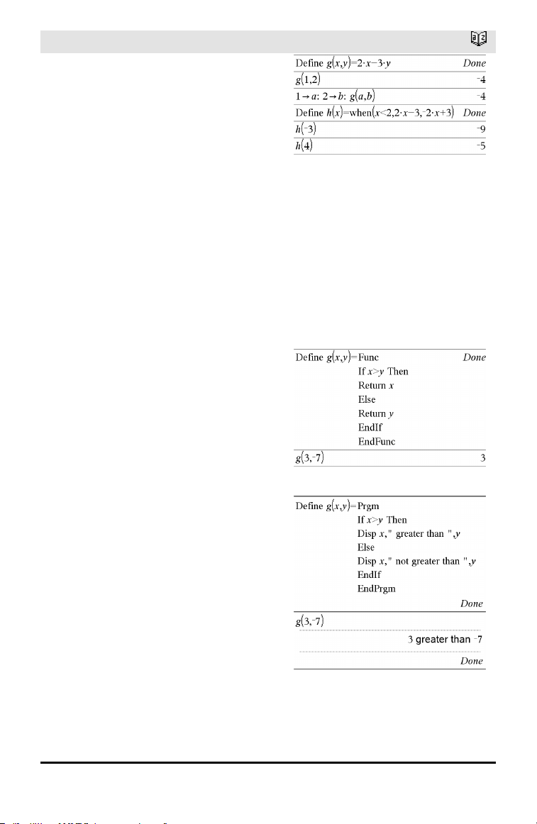
dbd()
Catalog >
dbd(date1,date2) ⇒ value
Returns the number of days between date1
and date2 using the actual-day-count
method.
date1 and date2 can be numbers or lists of
numbers within the range of the dates on
the standard calendar. If both date1 and
date2 are lists, they must be the same
length.
date1 and date2 must be between the
years 1950 through 2049.
dbd()
Catalog >
You can enter the dates in either of two
formats. The decimal placement
differentiates between the date formats.
MM.DDYY (format used commonly in the
United States)
DDMM.YY (format use commonly in
Europe)
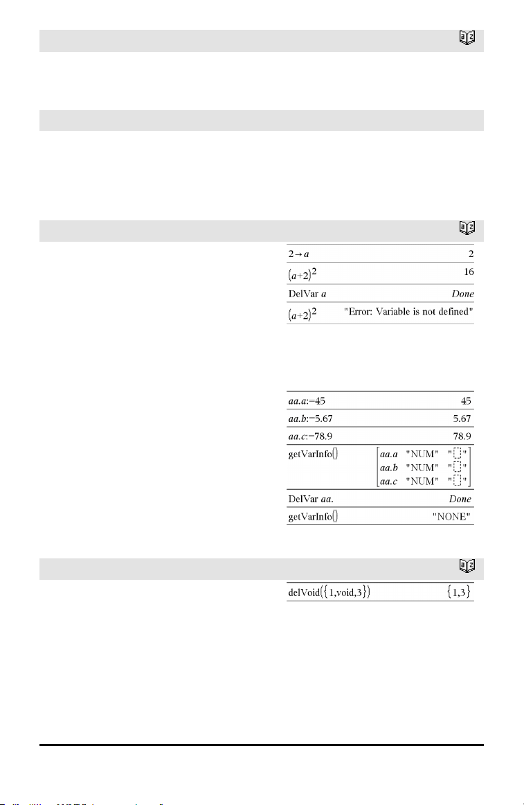
►DD
Catalog >
Expr1 ►DD ⇒ valueList1
►DD ⇒ listMatrix1
►DD ⇒ matrix
Note: You can insert this operator from the
computer keyboard by typing @>DD.
Returns the decimal equivalent of the
argument expressed in degrees. The
argument is a number, list, or matrix that is
interpreted by the Angle mode setting in
gradians, radians or degrees.
In Degree angle mode:
In Gradian angle mode:
In Radian angle mode:
►Decimal
Catalog >
Number1 ►Decimal ⇒ value
List1 ►Decimal ⇒ value
Matrix1 ►Decimal ⇒ value
Note: You can insert this operator from the
computer keyboard by typing @>Decimal.
Displays the argument in decimal form.
This operator can be used only at the end of
the entry line.
Define
Catalog >
Define Var = Expression
Alphabetical Listing 35
36 Alphabetical Listing
Define
Catalog >
Define Function(Param1, Param2, ...) =
Expression
Defines the variable Var or the user-
defined function Function.
Parameters, such as Param1, provide
placeholders for passing arguments to the
function. When calling a user-defined
function, you must supply arguments (for
example, values or variables) that
correspond to the parameters. When called,
the function evaluates Expression using
the supplied arguments.
Var and Function cannot be the name of a
system variable or built-in function or
command.
Note: This form of Define is equivalent to
executing the expression: expression →
Function(Param1,Param2).
Define Function(Param1, Param2, ...) =
Func
Block
EndFunc
Define Program(Param1, Param2, ...) =
Prgm
Block
EndPrgm
In this form, the user-defined function or
program can execute a block of multiple
statements.
Block can be either a single statement or a
series of statements on separate lines.
Block also can include expressions and
instructions (such as If, Then, Else, and For).
Note for entering the example: For
instructions on entering multi-line program
and function definitions, refer to the
Calculator section of your product
guidebook.

Define
Catalog >
Note: See also Define LibPriv, page 37, and
Define LibPub, page 37.
Define LibPriv
Catalog >
Define LibPriv Var = Expression
Define LibPriv Function(Param1, Param2,
...) = Expression
Define LibPriv Function(Param1, Param2,
...) = Func
Block
EndFunc
Define LibPriv Program(Param1, Param2,
...) = Prgm
Block
EndPrgm
Operates the same as Define, except defines
a private library variable, function, or
program. Private functions and programs do
not appear in the Catalog.
Note: See also Define, page 35, and Define
LibPub, page 37.
Define LibPub
Catalog >
Define LibPub Var = Expression
Define LibPub Function(Param1, Param2,
...) = Expression
Define LibPub Function(Param1, Param2,
...) = Func
Block
EndFunc
Define LibPub Program(Param1, Param2,
...) = Prgm
Block
EndPrgm
Operates the same as Define, except defines
a public library variable, function, or
program. Public functions and programs
appear in the Catalog after the library has
been saved and refreshed.
Alphabetical Listing 37
38 Alphabetical Listing
Define LibPub
Catalog >
Note: See also Define, page 35, and Define
LibPriv, page 37.
deltaList()
See ΔList(), page 82.
DelVar
Catalog >
DelVar Var1[, Var2] [, Var3] ...
DelVar Var.
Deletes the specified variable or variable
group from memory.
If one or more of the variables are locked,
this command displays an error message
and deletes only the unlocked variables. See
unLock, page 163.
DelVar Var. deletes all members of the
Var. variable group (such as the statistics
stat.nn results or variables created using
the LibShortcut() function). The dot (.) in
this form of the DelVar command limits it
to deleting a variable group; the simple
variable Var is not affected.
delVoid()
Catalog >
delVoid(List1) ⇒ list
Returns a list that has the contents of List1
with all empty (void) elements removed.
For more information on empty elements,
see page 196.
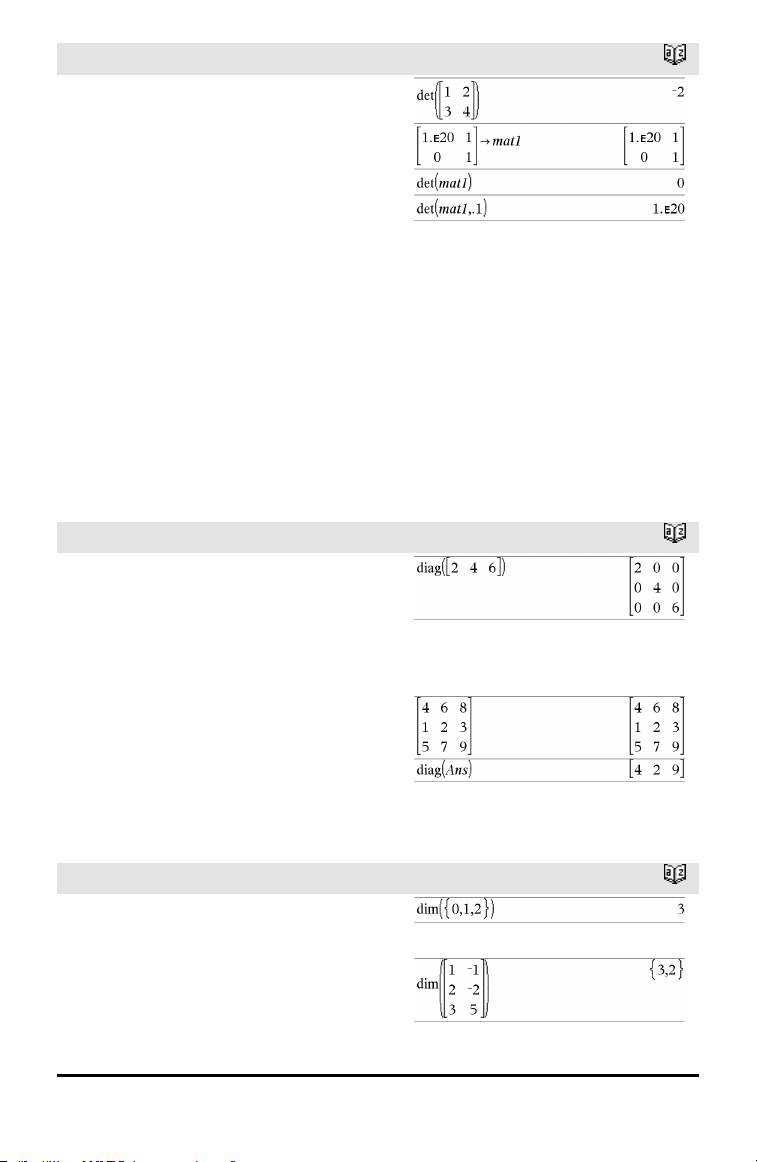
det()
Catalog >
det(squareMatrix[, Tolerance]) ⇒
expression
Returns the determinant of squareMatrix.
Optionally, any matrix element is treated as
zero if its absolute value is less than
Tolerance. This tolerance is used only if the
matrix has floating-point entries and does
not contain any symbolic variables that
have not been assigned a value. Otherwise,
Tolerance is ignored.
• If you use /· or set the Auto or
Approximate mode to Approximate,
computations are done using floating-
point arithmetic.
• If Tolerance is omitted or not used, the
default tolerance is calculated as:
5E⁻14 •max(dim(squareMatrix))
•rowNorm(squareMatrix)
diag()
Catalog >
diag(List) ⇒ matrix
diag(rowMatrix) ⇒ matrix
diag(columnMatrix) ⇒ matrix
Returns a matrix with the values in the
argument list or matrix in its main
diagonal.
diag(squareMatrix) ⇒ rowMatrix
Returns a row matrix containing the
elements from the main diagonal of
squareMatrix.
squareMatrix must be square.
dim()
Catalog >
dim(List) ⇒ integer
Returns the dimension of List.
dim(Matrix) ⇒ list
Returns the dimensions of matrix as a two-
element list {rows, columns}.
Alphabetical Listing 39
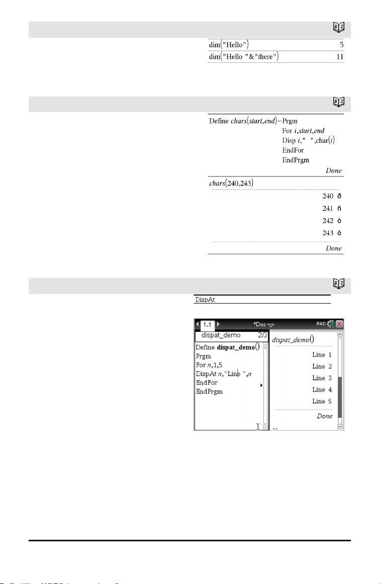
40 Alphabetical Listing
dim()
Catalog >
dim(String) ⇒ integer
Returns the number of characters contained
in character string String.
Disp
Catalog >
Disp exprOrString1 [, exprOrString2] ...
Displays the arguments in the Calculator
history. The arguments are displayed in
succession, with thin spaces as separators.
Useful mainly in programs and functions to
ensure the display of intermediate
calculations.
Note for entering the example: For
instructions on entering multi-line program
and function definitions, refer to the
Calculator section of your product
guidebook.
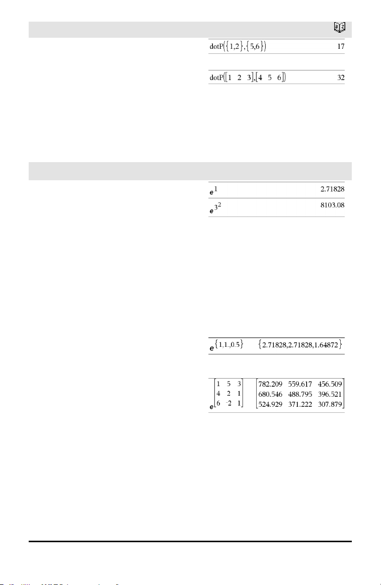
DispAt
Catalog >
DispAt int,expr1 [,expr2 ...] ...
DispAt allows you to specify the line
where the specified expression or string
will be displayed on the screen.
The line number can be specified as an
expression.
Please note that the line number is not
for the entire screen but for the area
immediately following the
command/program.
This command allows dashboard-like
output from programs where the value
of an expression or from a sensor
reading is updated on the same line.
DispAtand Disp can be used within the
same program.
Example
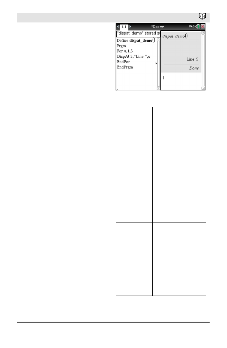
DispAt
Catalog >
Note: The maximum number is set to 8
since that matches a screen-full of lines
on the handheld screen - as long as the
lines don't have 2D math expressions.
The exact number of lines depends on
the content of the displayed
information.
Illustrative examples:
Define z()=
Prgm
For n,1,3
DispAt 1,"N: ",n
Disp "Hello"
EndFor
EndPrgm
Output
z()
Iteration 1:
Line 1: N:1
Line 2: Hello
Iteration 2:
Line 1: N:2
Line 2: Hello
Line 3: Hello
Iteration 3:
Line 1: N:3
Line 2: Hello
Line 3: Hello
Line 4: Hello
Define z1()=
Prgm
For n,1,3
DispAt 1,"N: ",n
EndFor
For n,1,4
Disp "Hello"
EndFor
EndPrgm
z1()
Line 1: N:3
Line 2: Hello
Line 3: Hello
Line 4: Hello
Line 5: Hello
Alphabetical Listing 41

42 Alphabetical Listing
DispAt
Catalog >
Error conditions:
Error Message Description
DispAt line number must be between 1 and 8 Expression evaluates the line number
outside the range 1-8 (inclusive)
Too few arguments The function or command is missing one
or more arguments.
No arguments Same as current 'syntax error' dialog
Too many arguments Limit argument. Same error as Disp.
Invalid data type First argument must be a number.
Void: DispAt void "Hello World" Datatype error is thrown
for the void (if the callback is defined)
►DMS
Catalog >
Value ►DMS
List ►DMS
Matrix ►DMS
Note: You can insert this operator from the
computer keyboard by typing @>DMS.
Interprets the argument as an angle and
displays the equivalent DMS
(DDDDDD°MM'SS.ss'') number. See °, ', ''
on page 190 for DMS (degree, minutes,
seconds) format.
Note: ►DMS will convert from radians to
degrees when used in radian mode. If the
input is followed by a degree symbol ° , no
conversion will occur. You can use ►DMS
only at the end of an entry line.
In Degree angle mode:
dotP()
Catalog >
dotP(List1, List2) ⇒ expression
Returns the “dot” product of two lists.
dotP(Vector1, Vector2) ⇒ expression
Returns the “dot” product of two vectors.
Both must be row vectors, or both must be
column vectors.
E
e^()
u key
e^(Value1) ⇒ value
Returns e raised to the Value1 power.
Note: See also e exponent template, page
2.
Note: Pressing u to display e^( is different
from pressing the character E on the
keyboard.
You can enter a complex number in re
i
θ
polar form. However, use this form in
Radian angle mode only; it causes a
Domain error in Degree or Gradian angle
mode.
e^(List1) ⇒ list
Returns e raised to the power of each
element in List1.
e^(squareMatrix1) ⇒ squareMatrix
Returns the matrix exponential of
squareMatrix1. This is not the same as
calculating e raised to the power of each
element. For information about the
calculation method, refer to cos().
squareMatrix1 must be diagonalizable. The
result always contains floating-point
numbers.
Alphabetical Listing 43
44 Alphabetical Listing
eff()
Catalog >
eff(nominalRate,CpY) ⇒ value
Financial function that converts the nominal
interest rate nominalRate to an annual
effective rate, given CpY as the number of
compounding periods per year.
nominalRate must be a real number, and
CpY must be a real number > 0.
Note: See also nom(), page 102.
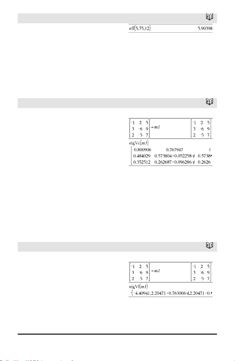
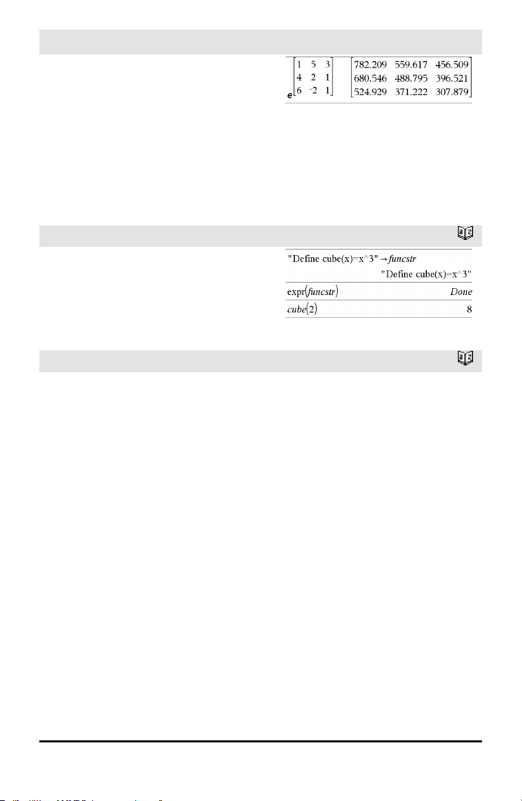
eigVc()
Catalog >
eigVc(squareMatrix) ⇒ matrix
Returns a matrix containing the
eigenvectors for a real or complex
squareMatrix, where each column in the
result corresponds to an eigenvalue. Note
that an eigenvector is not unique; it may be
scaled by any constant factor. The
eigenvectors are normalized, meaning that:
if V = [x
1
, x
2
, … , x
n
]
then x
1
2
+x
2
2
+ … +x
n
2
= 1
squareMatrix is first balanced with
similarity transformations until the row and
column norms are as close to the same
value as possible. The squareMatrix is then
reduced to upper Hessenberg form and the
eigenvectors are computed via a Schur
factorization.
In Rectangular Complex Format:
To see the entire result, press £ and then
use ¡and¢ to move the cursor.
eigVl()
Catalog >
eigVl(squareMatrix) ⇒ list
Returns a list of the eigenvalues of a real or
complex squareMatrix.
squareMatrix is first balanced with
similarity transformations until the row and
column norms are as close to the same
value as possible. The squareMatrix is then
reduced to upper Hessenberg form and the
eigenvalues are computed from the upper
Hessenberg matrix.
In Rectangular complex format mode:
To see the entire result, press £ and then
use ¡and¢ to move the cursor.

Else
See If, page 67.
ElseIf
Catalog >
If BooleanExpr1 Then
Block1
ElseIf BooleanExpr2 Then
Block2
⋮
ElseIf BooleanExprN Then
BlockN
EndIf
⋮
Note for entering the example: For
instructions on entering multi-line program
and function definitions, refer to the
Calculator section of your product
guidebook.
EndFor
See For, page 53.
EndFunc
See Func, page 57.
EndIf
See If, page 67.
EndLoop
See Loop, page 89.
EndPrgm
See Prgm, page 113.
EndTry
See Try, page 157.
Alphabetical Listing 45
46 Alphabetical Listing
EndWhile
See While, page 166.
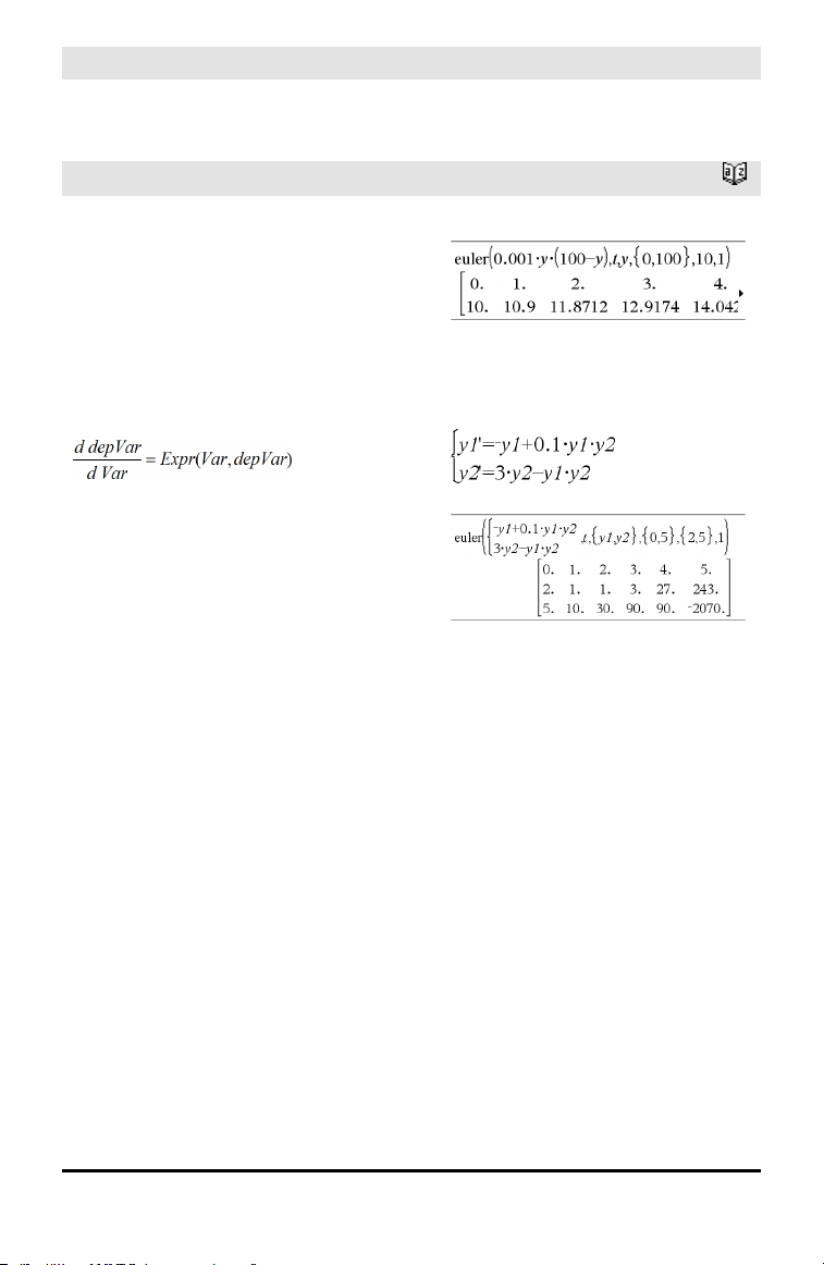
euler ()
Catalog >
euler(Expr, Var, depVar, {Var0, VarMax},
depVar0, VarStep [, eulerStep]) ⇒ matrix
euler(SystemOfExpr, Var, ListOfDepVars,
{Var0, VarMax}, ListOfDepVars0,
VarStep [, eulerStep]) ⇒ matrix
euler(ListOfExpr, Var, ListOfDepVars,
{Var0, VarMax},ListOfDepVars0,
VarStep [, eulerStep]) ⇒ matrix
Uses the Euler method to solve the system
with depVar(Var0)=depVar0 on the
interval [Var0,VarMax]. Returns a matrix
whose first row defines the Var output
values and whose second row defines the
value of the first solution component at the
corresponding Var values, and so on.
Expr is the right-hand side that defines the
ordinary differential equation (ODE).
SystemOfExpr is the system of right-hand
sides that define the system of ODEs
(corresponds to order of dependent
variables in ListOfDepVars).
ListOfExpr is a list of right-hand sides that
define the system of ODEs (corresponds to
the order of dependent variables in
ListOfDepVars).
Var is the independent variable.
ListOfDepVars is a list of dependent
variables.
{Var0, VarMax} is a two-element list that
tells the function to integrate from Var0 to
VarMax.
ListOfDepVars0 is a list of initial values
for dependent variables.
Differential equation:
y'=0.001*y*(100-y) andy(0)=10
To see the entire result, press £ and then
use ¡and¢ to move the cursor.
System of equations:
withy1(0)=2 and y2(0)=5
euler ()
Catalog >
VarStep is a nonzero number such that sign
(VarStep) = sign(VarMax-Var0) and
solutions are returned at Var0+i•VarStep
for all i=0,1,2,… such that Var0+i•VarStep
is in [var0,VarMax] (there may not be a
solution value at VarMax).
eulerStep is a positive integer (defaults to
1) that defines the number of euler steps
between output values. The actual step size
used by the euler method is
VarStep⁄ eulerStep.
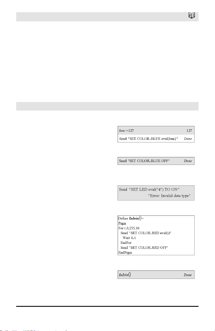
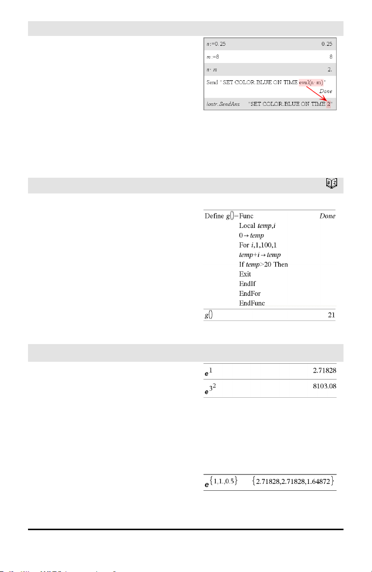
eval () Hub Menu
eval(Expr) ⇒ string
eval() is valid only in the TI-Innovator™ Hub
Command argument of programming
commands Get, GetStr, and Send. The
software evaluates expression Expr and
replaces the eval() statement with the
result as a character string.
The argument Expr must simplify to a real
number.
Set the blue element of the RGB LED to half
intensity.
Reset the blue element to OFF.
eval() argument must simplify to a real
number.
Program to fade-in the red element
Execute the program.
Alphabetical Listing 47
48 Alphabetical Listing
eval () Hub Menu
Although eval() does not display its result,
you can view the resulting Hub command
string after executing the command by
inspecting any of the following special
variables.
iostr.SendAns
iostr.GetAns
iostr.GetStrAns
Note: See also Get(page 58), GetStr(page
65), and Send(page 134).
Exit
Catalog >
Exit
Exits the current For, While, or Loop block.
Exit is not allowed outside the three looping
structures (For, While, or Loop).
Note for entering the example: For
instructions on entering multi-line program
and function definitions, refer to the
Calculator section of your product
guidebook.
Function listing:
exp()
u key
exp(Value1) ⇒ value
Returns e raised to the Value1 power.
Note: See also e exponent template, page
2.
You can enter a complex number in re
i
θ
polar form. However, use this form in
Radian angle mode only; it causes a
Domain error in Degree or Gradian angle
mode.
exp(List1) ⇒ list
Returns e raised to the power of each
element in List1.
exp()
u key
exp(squareMatrix1) ⇒ squareMatrix
Returns the matrix exponential of
squareMatrix1. This is not the same as
calculating e raised to the power of each
element. For information about the
calculation method, refer to cos().
squareMatrix1 must be diagonalizable. The
result always contains floating-point
numbers.
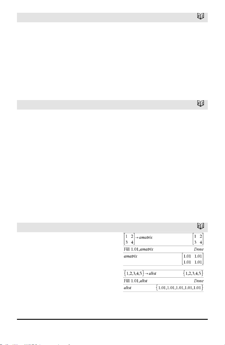
expr()
Catalog >
expr(String) ⇒ expression
Returns the character string contained in
String as an expression and immediately
executes it.
ExpReg
Catalog >
ExpReg X, Y [, [Freq] [, Category,
Include]]
Computes the exponential regression y = a•
(b)
x
on lists X and Y with frequency Freq. A
summary of results is stored in the
stat.results variable. (See page 145.)
All the lists must have equal dimension
except for Include.
X and Y are lists of independent and
dependent variables.
Freq is an optional list of frequency values.
Each element in Freq specifies the
frequency of occurrence for each
corresponding X and Y data point. The
default value is 1. All elements must be
integers ≥ 0.
Category is a list of numeric or string
category codes for the corresponding X and
Y data.
Alphabetical Listing 49

50 Alphabetical Listing
ExpReg
Catalog >
Include is a list of one or more of the
category codes. Only those data items
whose category code is included in this list
are included in the calculation.
For information on the effect of empty
elements in a list, see “Empty (Void)
Elements,” page 196.
Output
variable
Description
stat.RegEqn
Regression equation: a•(b)
x
stat.a, stat.b Regression coefficients
stat.r
2
Coefficientof linear determination for transformeddata
stat.r Correlation coefficient for transformed data (x, ln(y))
stat.Resid Residuals associated with the exponential model
stat.ResidTrans Residuals associated with linear fitof transformed data
stat.XReg
Listof data points in the modifiedX List actually used in the regression based on
restrictions of Freq, Category List, and Include Categories
stat.YReg
Listof data points in the modifiedY List actually used inthe regression basedon
restrictions of Freq, Category List, and Include Categories
stat.FreqReg
Listof frequencies corresponding to stat.XReg and stat.YReg
F
factor()
Catalog >
factor(rationalNumber) returns the rational
number factored into primes. For
composite numbers, the computing time
grows exponentially with the number of
digits in the second-largest factor. For
example, factoring a 30-digit integer could
take more than a day, and factoring a 100-
digit number could take more than a
century.
To stop a calculation manually,
• Handheld: Hold down the c key and
press · repeatedly.
• Windows®: Hold down the F12 key and
factor()
Catalog >
press Enter repeatedly.
• Macintosh®: Hold down the F5 key and
press Enter repeatedly.
• iPad®: The app displays a prompt. You
can continue waiting or cancel.
If you merely want to determine if a
number is prime, use isPrime() instead. It is
much faster, particularly if rationalNumber
is not prime and if the second-largest factor
has more than five digits.
FCdf()
Catalog >
FCdf
(lowBound,upBound,dfNumer,dfDenom) ⇒
number if lowBound and upBound are
numbers, list if lowBound and upBound are
lists
FCdf
(lowBound,upBound,dfNumer,dfDenom) ⇒
number if lowBound and upBound are
numbers, list if lowBound and upBound are
lists
Computes the F distribution probability
between lowBound and upBound for the
specified dfNumer (degrees of freedom) and
dfDenom.
For P(X ≤ upBound), set lowBound = 0.
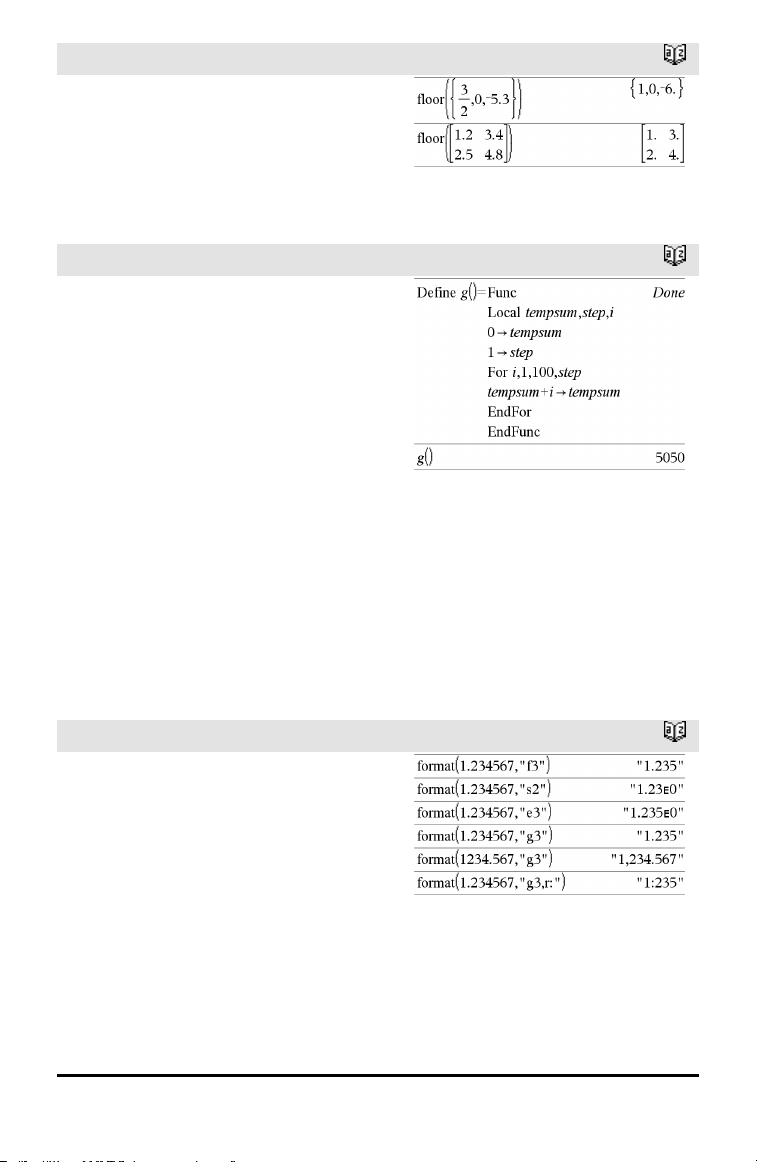
Fill
Catalog >
Fill Value, matrixVar ⇒ matrix
Replaces each element in variable
matrixVar with Value.
matrixVar must already exist.
Fill Value, listVar ⇒ list
Replaces each element in variable listVar
with Value.
listVar must already exist.
Alphabetical Listing 51

52 Alphabetical Listing
FiveNumSummary
Catalog >
FiveNumSummary X[,[Freq]
[,Category,Include]]
Provides an abbreviated version of the 1-
variable statistics on list X. Asummary of
results is stored in the stat.results variable.
(See page 145.)
X represents a list containing the data.
Freq is an optional list of frequency values.
Each element in Freq specifies the
frequency of occurrence for each
corresponding X and Y data point. The
default value is 1.
Category is a list of numeric category codes
for the corresponding X data.
Include is a list of one or more of the
category codes. Only those data items
whose category code is included in this list
are included in the calculation.
An empty (void) element in any of the lists
X, Freq, or Category results in a void for
the corresponding element of all those lists.
For more information on empty elements,
see page 196.
Output variable Description
stat.MinX Minimum of x values.
stat.Q
1
X 1st Quartile of x.
stat.MedianX Median of x.
stat.Q
3
X 3rd Quartile of x.
stat.MaxX Maximum of x values.
floor()
Catalog >
floor(Value1) ⇒ integer
Returns the greatest integer that is ≤ the
argument. This function is identical to int().
The argument can be a real or a complex
number.
floor()
Catalog >
floor(List1) ⇒ list
floor(Matrix1) ⇒ matrix
Returns a list or matrix of the floor of each
element.
Note: See also ceiling() and int().
For
Catalog >
For Var, Low, High [, Step]
Block
EndFor
Executes the statements in Block
iteratively for each value of Var, from Low
to High, in increments of Step.
Var must not be a system variable.
Step can be positive or negative. The
default value is 1.
Block can be either a single statement or a
series of statements separated with the “:”
character.
Note for entering the example: For
instructions on entering multi-line program
and function definitions, refer to the
Calculator section of your product
guidebook.
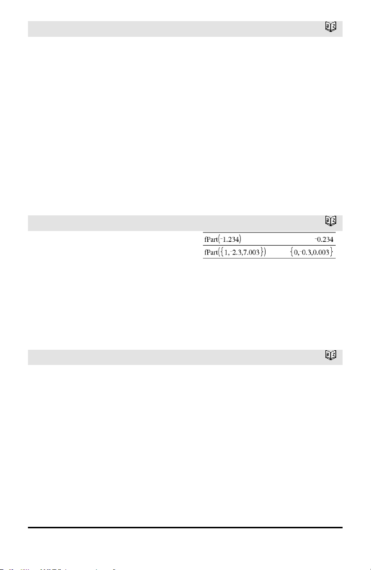
format()
Catalog >
format(Value[, formatString]) ⇒ string
Returns Value as a character string based
on the format template.
formatString is a string and must be in the
form: “F[n]”, “S[n]”, “E[n]”, “G[n][c]”,
where [] indicate optional portions.
F[n]: Fixed format. n is the number of digits
to display after the decimal point.
S[n]: Scientific format. n is the number of
digits to display after the decimal point.
Alphabetical Listing 53
54 Alphabetical Listing
format()
Catalog >
E[n]: Engineering format. n is the number
of digits after the first significant digit. The
exponent is adjusted to a multiple of three,
and the decimal point is moved to the right
by zero, one, or two digits.
G[n][c]: Same as fixed format but also
separates digits to the left of the radix into
groups of three. c specifies the group
separator character and defaults to a
comma. If c is a period, the radix will be
shown as a comma.
[Rc]: Any of the above specifiers may be
suffixed with the Rc radix flag, where c is a
single character that specifies what to
substitute for the radix point.
fPart()
Catalog >
fPart(Expr1) ⇒ expression
fPart(List1) ⇒ list
fPart(Matrix1) ⇒ matrix
Returns the fractional part of the argument.
For a list or matrix, returns the fractional
parts of the elements.
The argument can be a real or a complex
number.
FPdf()
Catalog >
FPdf(XVal,dfNumer,dfDenom) ⇒ number
if XVal is a number, list if XVal is a list
Computes the F distribution probability at
XVal for the specified dfNumer (degrees of
freedom) and dfDenom.
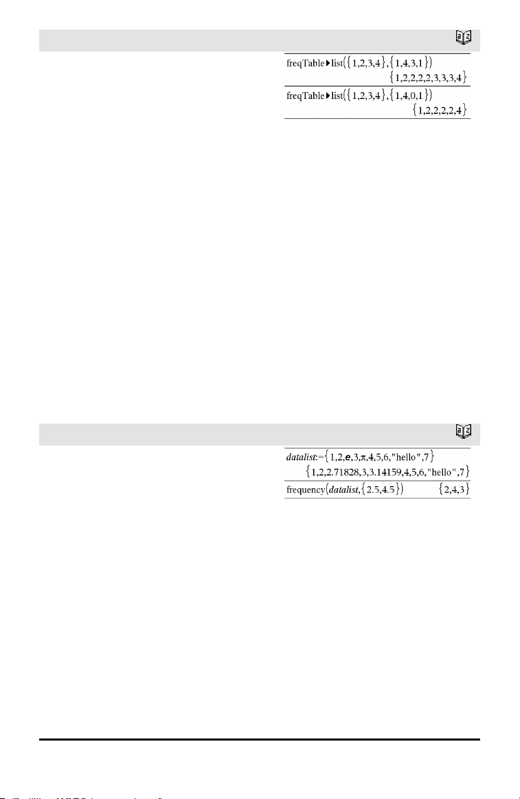
freqTable►list()
Catalog >
freqTable►list(List1,freqIntegerList) ⇒
list
Returns a list containing the elements from
List1 expanded according to the
frequencies in freqIntegerList. This
function can be used for building a
frequency table for the Data & Statistics
application.
List1 can be any valid list.
freqIntegerList must have the same
dimension as List1 and must contain non-
negative integer elements only. Each
element specifies the number of times the
corresponding List1 element will be
repeated in the result list. A value of zero
excludes the corresponding List1 element.
Note: You can insert this function from the
computer keyboard by typing
freqTable@>list(...).
Empty (void) elements are ignored. For
more information on empty elements, see
page 196.
frequency()
Catalog >
frequency(List1,binsList) ⇒ list
Returns a list containing counts of the
elements in List1. The counts are based on
ranges (bins) that you define in binsList.
If binsList is {b(1), b(2), …, b(n)}, the
specified ranges are {?≤b(1), b(1)<?≤b
(2),…,b(n-1)<?≤b(n), b(n)>?}. The resulting
list is one element longer than binsList.
Each element of the result corresponds to
the number of elements from List1 that
are in the range of that bin. Expressed in
terms of the countIf() function, the result is
{countIf(list, ?≤b(1)), countIf(list, b(1)<?≤b
(2)), …, countIf(list, b(n-1)<?≤b(n)), countIf
(list, b(n)>?)}.
Explanation of result:
2 elements from Datalist are ≤2.5
4 elements from Datalist are >2.5 and≤4.5
3 elements from Datalist are >4.5
The element“hello” is a string andcannot be
placed in any of the defined bins.
Alphabetical Listing 55

56 Alphabetical Listing
frequency()
Catalog >
Elements of List1 that cannot be “placed in
a bin” are ignored. Empty (void) elements
are also ignored. For more information on
empty elements, see page 196.
Within the Lists & Spreadsheet application,
you can use a range of cells in place of both
arguments.
Note: See also countIf(), page 29.
FTest_2Samp
Catalog >
FTest_2Samp List1,List2[,Freq1[,Freq2
[,Hypoth]]]
FTest_2Samp List1,List2[,Freq1[,Freq2
[,Hypoth]]]
(Data list input)
FTest_2Samp sx1,n1,sx2,n2[,Hypoth]
FTest_2Samp sx1,n1,sx2,n2[,Hypoth]
(Summary stats input)
Performs a two-sample Ftest. A summary
of results is stored in the stat.results
variable. (See page 145.)
For H
a
: σ1 > σ2, set Hypoth>0
For H
a
: σ1 ≠ σ2 (default), set Hypoth =0
For H
a
: σ1 < σ2, set Hypoth<0
For information on the effect of empty
elements in a list, see Empty (Void)
Elements, page 196.
Output variable Description
stat.F CalculatedF statistic for the data sequence
stat.PVal Smallest level of significance at whichthe null hypothesis can be rejected
stat.dfNumer numerator degrees of freedom = n1-1
stat.dfDenom denominator degrees of freedom = n2-1
stat.sx1, stat.sx2
Sample standard deviations of the data sequences inList1 and List2
Output variable Description
stat.x1_bar
stat.x2_bar
Sample means of the data sequences in List1 and List2
stat.n1, stat.n2 Size of the samples
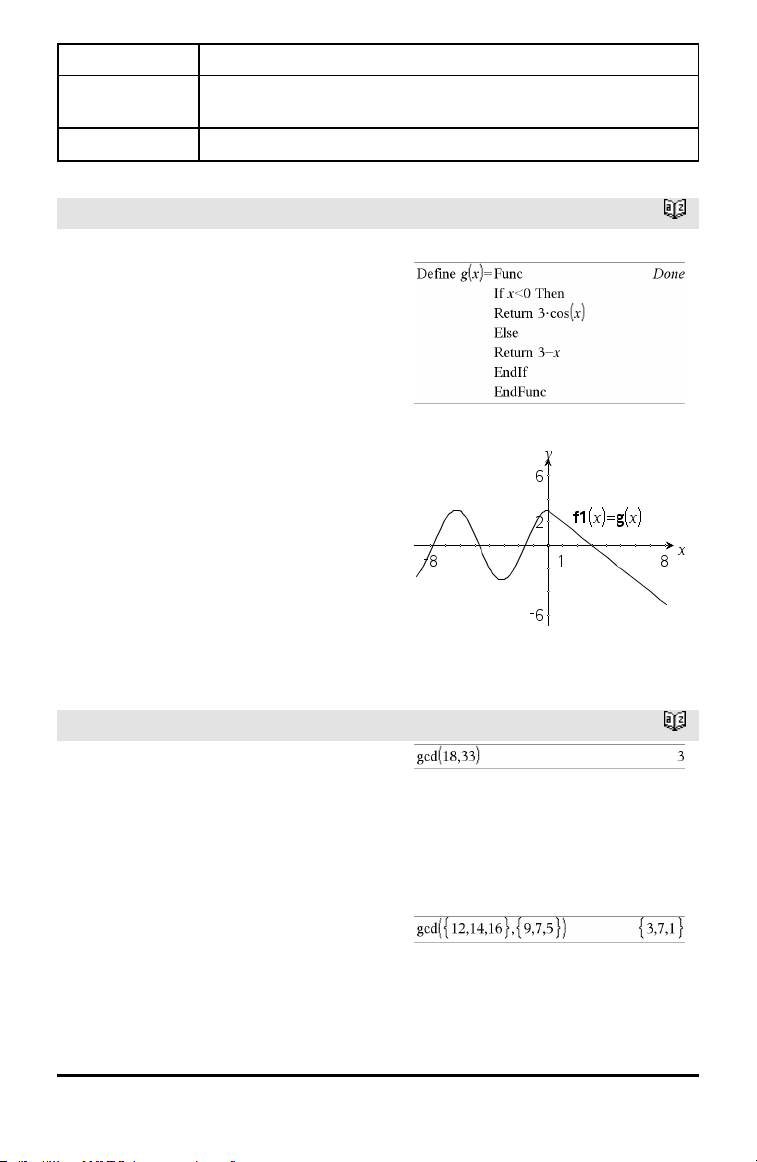
Func
Catalog >
Func
Block
EndFunc
Template for creating a user-defined
function.
Block can be a single statement, a series
of statements separated with the “:”
character, or a series of statements on
separate lines. The function can use the
Return instruction to return a specific result.
Note for entering the example: For
instructions on entering multi-line program
and function definitions, refer to the
Calculator section of your product
guidebook.
Define a piecewise function:
Resultof graphing g(x)
G
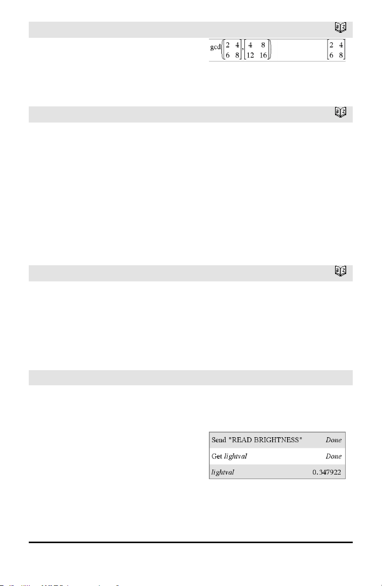
gcd()
Catalog >
gcd(Number1, Number2) ⇒ expression
Returns the greatest common divisor of the
two arguments. The gcd of two fractions is
the gcd of their numerators divided by the
lcm of their denominators.
In Auto or Approximate mode, the gcd of
fractional floating-point numbers is 1.0.
gcd(List1, List2) ⇒ list
Returns the greatest common divisors of
the corresponding elements in List1 and
List2.
Alphabetical Listing 57
58 Alphabetical Listing
gcd()
Catalog >
gcd(Matrix1, Matrix2) ⇒ matrix
Returns the greatest common divisors of
the corresponding elements in Matrix1and
Matrix2.
geomCdf()
Catalog >
geomCdf(p,lowBound,upBound) ⇒ number
if lowBound and upBound are numbers, list
if lowBound and upBound are lists
geomCdf(p,upBound)for P(1≤X≤upBound)
⇒ number if upBound is a number, list if
upBound is a list
Computes a cumulative geometric
probability from lowBound to upBound with
the specified probability of success p.
For P(X ≤ upBound), set lowBound = 1.
geomPdf()
Catalog >
geomPdf(p,XVal) ⇒ number if XVal is a
number, list if XVal is a list
Computes a probability at XVal, the number
of the trial on which the first success occurs,
for the discrete geometric distribution with
the specified probability of success p.
Get Hub Menu
Get [promptString,] var[,statusVar]
Get [promptString,] func(arg1, ...argn)
[,statusVar]
Programming command: Retrieves a value
from a connected TI-Innovator™ Hub and
assigns the value to variable var.
The value must be requested:
• In advance, through a Send"READ..."
command.
—or—
Example: Request the current value of the
hub's built-in light-level sensor. Use Get to
retrieve the value and assign it to variable
lightval.
Embed the READ request within the Get
command.
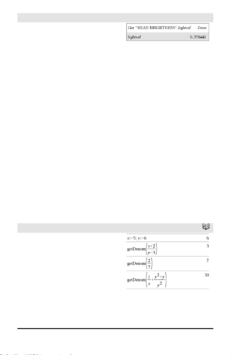
Get Hub Menu
• By embedding a "READ..." request as
the optional promptString argument.
This method lets you use a single
command to request the value and
retrieve it.
Implicit simplification takes place. For
example, a received string of "123" is
interpreted as a numeric value. To preserve
the string, use GetStr instead of Get.
If you include the optional argument
statusVar, it is assigned a value based on
the success of the operation. A value of
zero means that no data was received.
In the second syntax, the func() argument
allows a program to store the received
string as a function definition. This syntax
operates as if the program executed the
command:
Define func(arg1, ...argn) = received
string
The program can then use the defined
function func().
Note: You can use the Get command within
a user-defined program but not within a
function.
Note: See also GetStr, page 65 and Send,
page 134.
getDenom()
Catalog >
getDenom(Fraction1) ⇒ value
Transforms the argument into an
expression having a reduced common
denominator, and then returns its
denominator.
Alphabetical Listing 59

60 Alphabetical Listing
getKey()
Catalog >
getKey([0|1]) ⇒ returnString
Description:getKey() - allows a TI-Basic
program to get keyboard input -
handheld, desktop and emulator on
desktop.
Example:
• keypressed := getKey() will return a
key or an empty string if no key has
been pressed. This call will return
immediately.
• keypressed := getKey(1) will wait till
a key is pressed. This call will pause
execution of the program till a key is
pressed.
Example:
Handling of key presses:
Handheld Device/Emulator
Key
Desktop Return Value
Esc Esc "esc"
Touchpad - Top click n/a "up"
On n/a "home"
Scratchapps n/a "scratchpad"
Touchpad - Left click n/a "left"
Touchpad - Center click n/a "center"
Touchpad - Right click n/a "right"
Doc n/a "doc"
Tab Tab "tab"
Touchpad - Bottom click Down Arrow "down"
Menu n/a "menu"
Ctrl Ctrl no return
Shift Shift no return
Var n/a "var"

Handheld Device/Emulator
Key
Desktop Return Value
Del n/a "del"
= = "="
trig n/a "trig"
0 through 9 0-9 "0" ... "9"
Templates n/a "template"
Catalog n/a "cat"
^ ^ "^"
X^2 n/a "square"
/ (division key) / "/"
* (multiply key) * "*"
e^x n/a "exp"
10^x n/a "10power"
+ + "+"
- - "-"
( ( "("
) ) ")"
. . "."
(-) n/a "-" (negate sign)
Enter Enter "enter"
ee n/a "E" (scientific notation E)
a - z a-z alpha = letter pressed (lower
case)
("a" - "z")
shift a-z shift a-z alpha = letter pressed
"A" - "Z"
Note: ctrl-shift works to lock
caps
?! n/a "?!"
Alphabetical Listing 61

62 Alphabetical Listing
Handheld Device/Emulator
Key
Desktop Return Value
pi n/a "pi"
Flag n/a no return
, , ","
Return n/a "return"
Space Space " " (space)
Inaccessible Special Character Keys like
@,!,^, etc.
The character is returned
n/a Function Keys No returned character
n/a Special desktop control keys No returned character
Inaccessible Other desktop keys that are
not available on the
calculator while getkey() is
waiting for a keystroke. ({,
},;, :, ...)
Same character you get in
Notes (not in a math box)
Note: It is important to note that the presence of getKey() in a program changes how
certain events are handled by the system. Some of these are described below.
Terminate program and Handle event - Exactly as if the user were to break out of program
by pressing the ON key
"Support" below means - System works as expected - program continues to run.
Event Device Desktop - TI-Nspire™
Student Software
Quick Poll Terminate program,
handle event
Same as the handheld (TI-
Nspire™ Student Software,
TI-Nspire™ Navigator™ NC
Teacher Software-only)
Remote file mgmt
(Incl. sending 'Exit Press 2
Test' file from another
handheld or desktop-
handheld)
Terminate program,
handle event
Same as the handheld.
(TI-Nspire™ Student
Software, TI-Nspire™
Navigator™ NC Teacher
Software-only)
End Class Terminate program,
handle event
Support
(TI-Nspire™ Student
Software, TI-Nspire™
Navigator™ NC Teacher
Software-only)

Event Device Desktop - TI-Nspire™ All
Versions
TI-Innovator™ Hub
connect/disconnect
Support - Can successfully
issue commands to the TI-
Innovator™ Hub. After you
exit the program the TI-
Innovator™ Hub is still
working with the
handheld.
Same as the handheld
getLangInfo()
Catalog >
getLangInfo() ⇒ string
Returns a string that corresponds to the
short name of the currently active
language. You can, for example, use it in a
program or function to determine the
current language.
English = “en”
Danish = “da”
German = “de”
Finnish = “fi”
French = “fr”
Italian = “it”
Dutch = “nl”
Belgian Dutch = “nl_BE”
Norwegian = “no”
Portuguese = “pt”
Spanish = “es”
Swedish = “sv”
getLockInfo()
Catalog >
getLockInfo(Var) ⇒ value
Returns the current locked/unlocked state
of variable Var.
value =0: Var is unlocked or does not exist.
value =1: Var is locked and cannot be
modified or deleted.
See Lock, page 85, and unLock, page 163.
Alphabetical Listing 63

64 Alphabetical Listing
getMode()
Catalog >
getMode(ModeNameInteger) ⇒ value
getMode(0) ⇒ list
getMode(ModeNameInteger) returns a
value representing the current setting of
the ModeNameInteger mode.
getMode(0) returns a list containing
number pairs. Each pair consists of a mode
integer and a setting integer.
For a listing of the modes and their
settings, refer to the table below.
If you save the settings with getMode(0) →
var, you can use setMode(var) in a function
or program to temporarily restore the
settings within the execution of the
function or program only. See setMode(),
page 136.
Mode
Name
Mode
Integer Setting Integers
Display
Digits
1
1=Float, 2=Float1, 3=Float2, 4=Float3, 5=Float4, 6=Float5,
7=Float6, 8=Float7, 9=Float8, 10=Float9, 11=Float10,
12=Float11, 13=Float12, 14=Fix0, 15=Fix1, 16=Fix2,
17=Fix3, 18=Fix4, 19=Fix5, 20=Fix6, 21=Fix7, 22=Fix8,
23=Fix9, 24=Fix10, 25=Fix11, 26=Fix12
Angle
2
1=Radian, 2=Degree, 3=Gradian
Exponential
Format
3
1=Normal, 2=Scientific, 3=Engineering
Real or
Complex
4
1=Real, 2=Rectangular, 3=Polar
Auto or
Approx.
5
1=Auto, 2=Approximate
Vector
Format
6
1=Rectangular, 2=Cylindrical, 3=Spherical
Base
7
1=Decimal, 2=Hex, 3=Binary
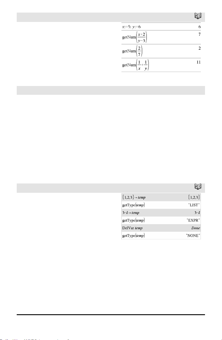
getNum()
Catalog >
getNum(Fraction1) ⇒ value
Transforms the argument into an
expression having a reduced common
denominator, and then returns its
numerator.
GetStr Hub Menu
GetStr [promptString,] var[, statusVar]
GetStr [promptString,] func(arg1, ...argn)
[,statusVar]
Programming command: Operates
identically to the Get command, except that
the retrieved value is always interpreted as
a string. By contrast, the Get command
interprets the response as an expression
unless it is enclosed in quotation marks ("").
Note: See also Get, page 58 and Send, page
134.
For examples, see Get.
getType()
Catalog >
getType(var) ⇒ string
Returns a string that indicates the data type
of variable var.
If var has not been defined, returns the
string "NONE".
Alphabetical Listing 65
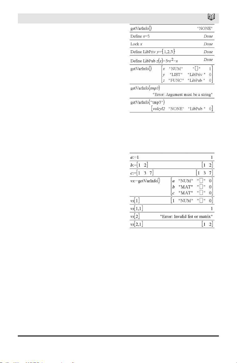
66 Alphabetical Listing
getVarInfo()
Catalog >
getVarInfo() ⇒ matrix or string
getVarInfo(LibNameString) ⇒ matrix or
string
getVarInfo() returns a matrix of information
(variable name, type, library accessibility,
and locked/unlocked state) for all variables
and library objects defined in the current
problem.
If no variables are defined, getVarInfo()
returns the string "NONE".
getVarInfo(LibNameString)returns a matrix
of information for all library objects defined
in library LibNameString. LibNameString
must be a string (text enclosed in quotation
marks) or a string variable.
If the library LibNameString does not exist,
an error occurs.
Note the example, in which the result of
getVarInfo() is assigned to variable vs.
Attempting to display row 2 or row 3 of vs
returns an “Invalid list or matrix” error
because at least one of elements in those
rows (variable b, for example) revaluates to
a matrix.
This error could also occur when using Ans
to reevaluate a getVarInfo() result.
The system gives the above error because
the current version of the software does not
support a generalized matrix structure
where an element of a matrix can be either
a matrix or a list.
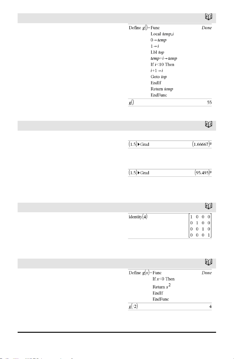
Goto
Catalog >
Goto labelName
Transfers control to the label labelName.
labelName must be defined in the same
function using a Lbl instruction.
Note for entering the example: For
instructions on entering multi-line program
and function definitions, refer to the
Calculator section of your product
guidebook.
►Grad
Catalog >
Expr1►Grad ⇒ expression
Converts Expr1 to gradian angle measure.
Note: You can insert this operator from the
computer keyboard by typing @>Grad.
In Degree angle mode:
In Radian angle mode:
I
identity()
Catalog >
identity(Integer) ⇒ matrix
Returns the identity matrix with a
dimension of Integer.
Integer must be a positive integer.
If
Catalog >
If BooleanExpr
Statement
If BooleanExpr Then
Block
EndIf
Alphabetical Listing 67
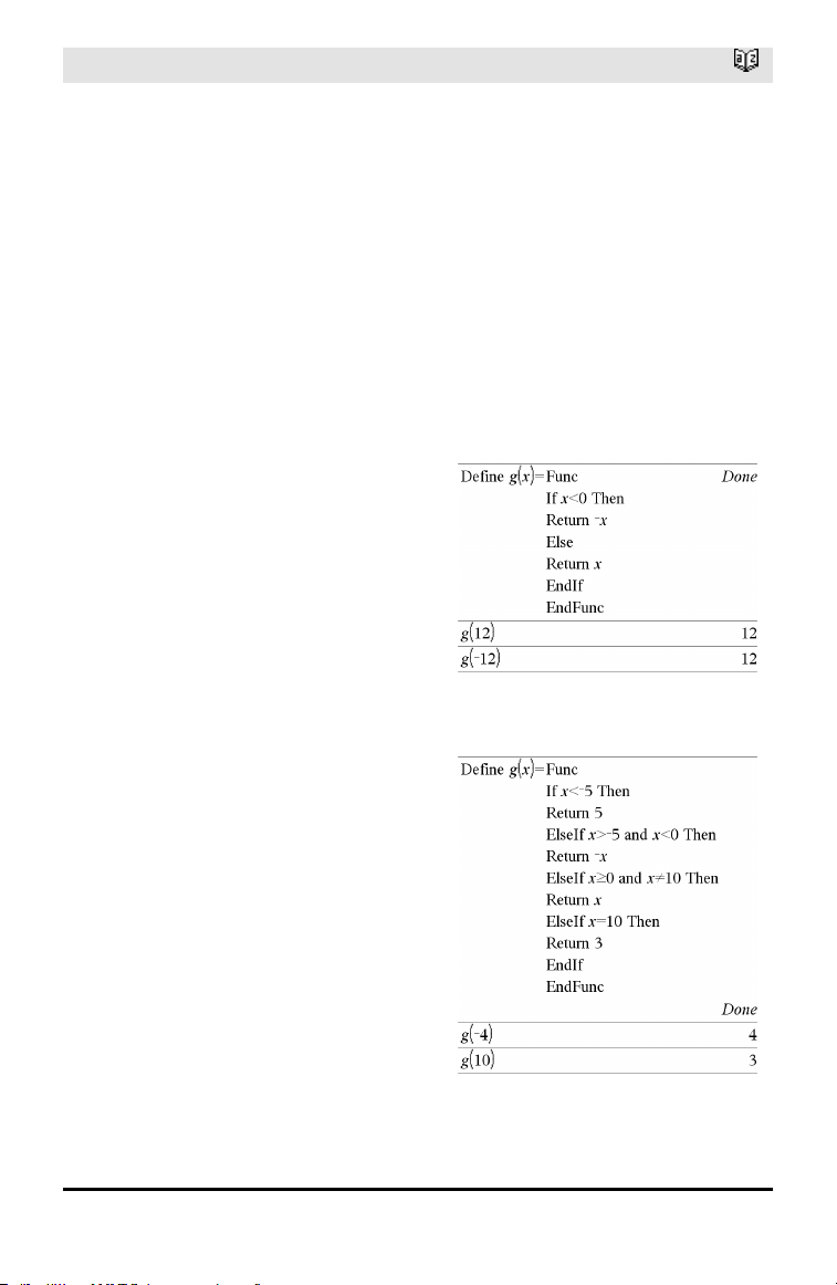
68 Alphabetical Listing
If
Catalog >
If BooleanExpr evaluates to true, executes
the single statement Statement or the block
of statements Block before continuing
execution.
If BooleanExpr evaluates to false,
continues execution without executing the
statement or block of statements.
Block can be either a single statement or a
sequence of statements separated with the
“:” character.
Note for entering the example: For
instructions on entering multi-line program
and function definitions, refer to the
Calculator section of your product
guidebook.
If BooleanExpr Then
Block1
Else
Block2
EndIf
If BooleanExpr evaluates to true, executes
Block1 and then skips Block2.
If BooleanExpr evaluates to false, skips
Block1 but executes Block2.
Block1 and Block2 can be a single
statement.
If BooleanExpr1 Then
Block1
ElseIf BooleanExpr2 Then
Block2
⋮
ElseIf BooleanExprN Then
BlockN
EndIf
Allows for branching. If BooleanExpr1
evaluates to true, executes Block1. If
BooleanExpr1 evaluates to false, evaluates
BooleanExpr2, and so on.
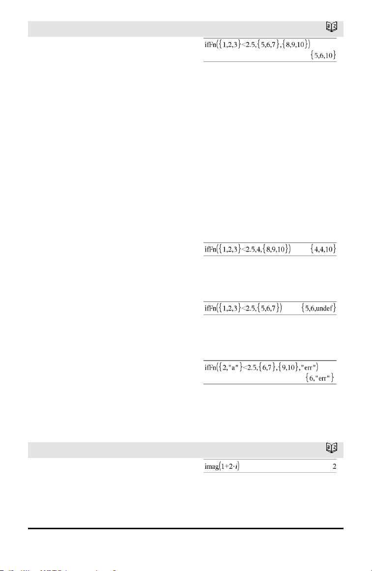
ifFn()
Catalog >
ifFn(BooleanExpr,Value_If_true [,Value_
If_false [,Value_If_unknown]]) ⇒
expression, list, or matrix
Evaluates the boolean expression
BooleanExpr (or each element from
BooleanExpr ) and produces a result based
on the following rules:
• BooleanExpr can test a single value, a
list, or a matrix.
• If an element of BooleanExpr evaluates
to true, returns the corresponding
element from Value_If_true.
• If an element of BooleanExpr evaluates
to false, returns the corresponding
element from Value_If_false. If you
omit Value_If_false, returns undef.
• If an element of BooleanExpr is neither
true nor false, returns the corresponding
element Value_If_unknown. If you omit
Value_If_unknown, returns undef.
• If the second, third, or fourth argument
of the ifFn() function is a single
expression, the Boolean test is applied to
every position in BooleanExpr.
Note: If the simplified BooleanExpr
statement involves a list or matrix, all other
list or matrix arguments must have the
same dimension(s), and the result will have
the same dimension(s).
Test value of 1 is less than 2.5, so its
corresponding
Value_If_True element of 5 is copiedto
the result list.
Test value of 2 is less than 2.5, so its
corresponding
Value_If_True element of 6 is copiedto
the result list.
Test value of 3 is not less than 2.5, so its
corresponding Value_If_False elementof
10 is copiedto the result list.
Value_If_true is a single value and
corresponds to any selectedposition.
Value_If_false is not specified. Undef is
used.
One element selectedfrom Value_If_true.
One element selectedfrom Value_If_
unknown.
imag()
Catalog >
imag(Value1) ⇒ value
Returns the imaginary part of the
argument.
Alphabetical Listing 69
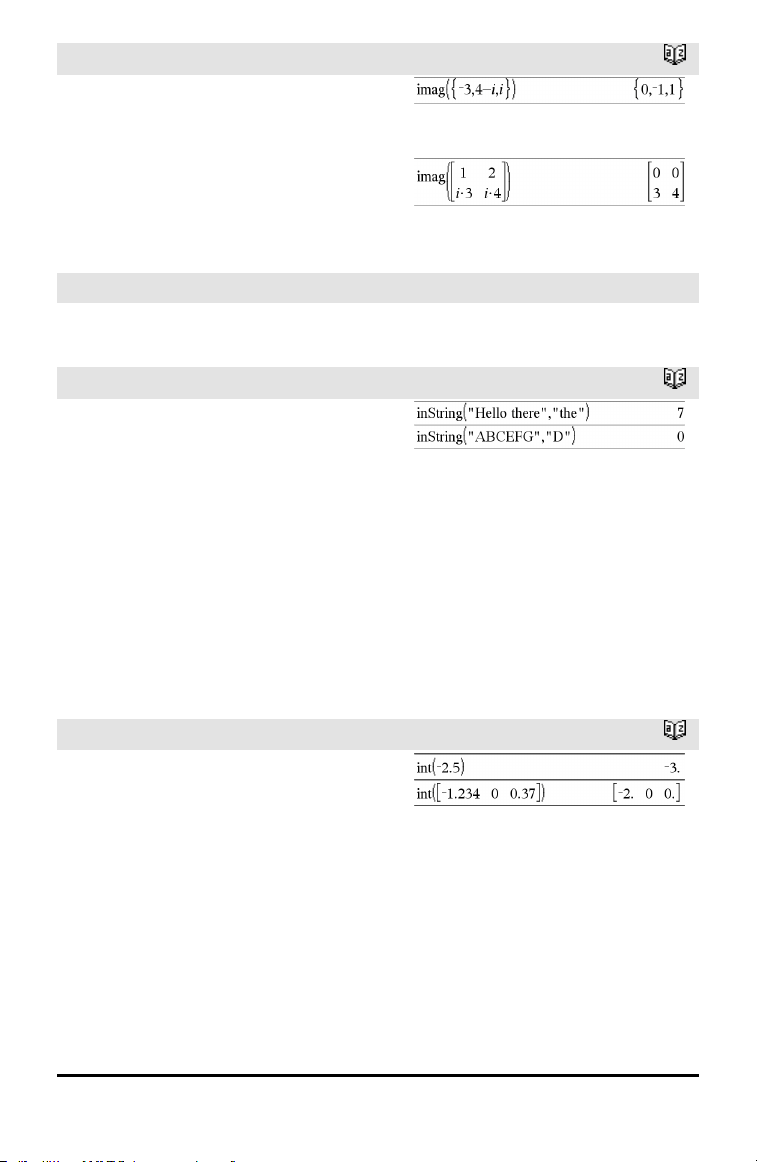
70 Alphabetical Listing
imag()
Catalog >
imag(List1) ⇒ list
Returns a list of the imaginary parts of the
elements.
imag(Matrix1) ⇒ matrix
Returns a matrix of the imaginary parts of
the elements.
Indirection
See #(), page 188.
inString()
Catalog >
inString(srcString, subString[, Start]) ⇒
integer
Returns the character position in string
srcString at which the first occurrence of
string subString begins.
Start, if included, specifies the character
position within srcString where the search
begins. Default = 1 (the first character of
srcString).
If srcString does not contain subString or
Start is > the length of srcString, returns
zero.
int()
Catalog >
int(Value) ⇒ integer
int(List1) ⇒ list
int(Matrix1) ⇒ matrix
Returns the greatest integer that is less
than or equal to the argument. This
function is identical to floor().
The argument can be a real or a complex
number.
For a list or matrix, returns the greatest
integer of each of the elements.
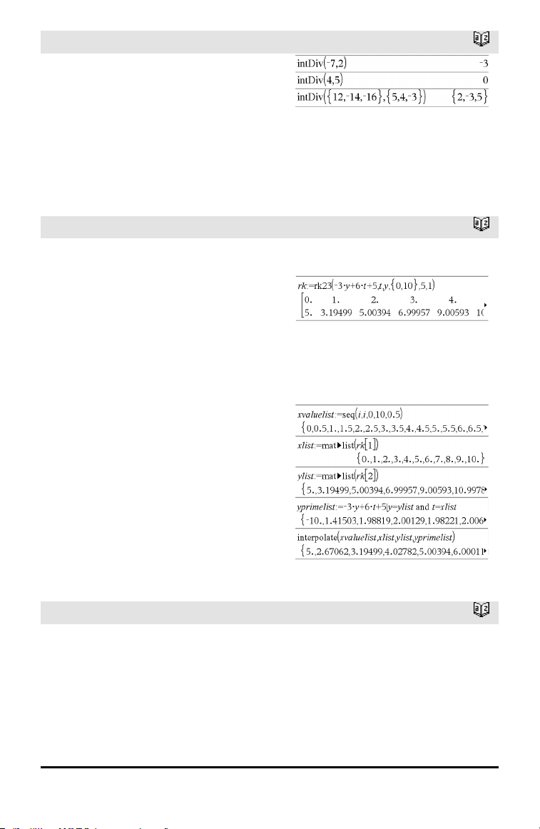
intDiv()
Catalog >
intDiv(Number1, Number2) ⇒ integer
intDiv(List1, List2) ⇒ list
intDiv(Matrix1, Matrix2) ⇒ matrix
Returns the signed integer part of
(Number1 ÷ Number2).
For lists and matrices, returns the signed
integer part of (argument1÷argument2)
for each element pair.
interpolate ()
Catalog >
interpolate(xValue, xList, yList,
yPrimeList) ⇒ list
This function does the following:
Given xList, yList=f(xList), and
yPrimeList=f'(xList) for some unknown
function f, a cubic interpolant is used to
approximate the function f at xValue. It is
assumed that xList is a list of
monotonically increasing or decreasing
numbers, but this function may return a
value even when it is not. This function
walks through xList looking for an interval
[xList[i], xList[i+1]] that contains xValue.
If it finds such an interval, it returns an
interpolated value for f(xValue); otherwise,
it returns undef.
xList, yList, and yPrimeList must be of
equal dimension ≥ 2 and contain
expressions that simplify to numbers.
xValue can be a number or a list of
numbers.
Differential equation:
y'=-3•y+6•t+5 and y(0)=5
To see the entire result, press £ and then
use ¡and¢ to move the cursor.
Use the interpolate() function to calculate the
function values for the xvaluelist:
invχ
2
()
Catalog >
invχ
2
(Area,df)
invChi2(Area,df)
Computes the Inverse cumulative χ
2
(chi-
square) probability function specified by
degree of freedom, df for a given Area
under the curve.
Alphabetical Listing 71
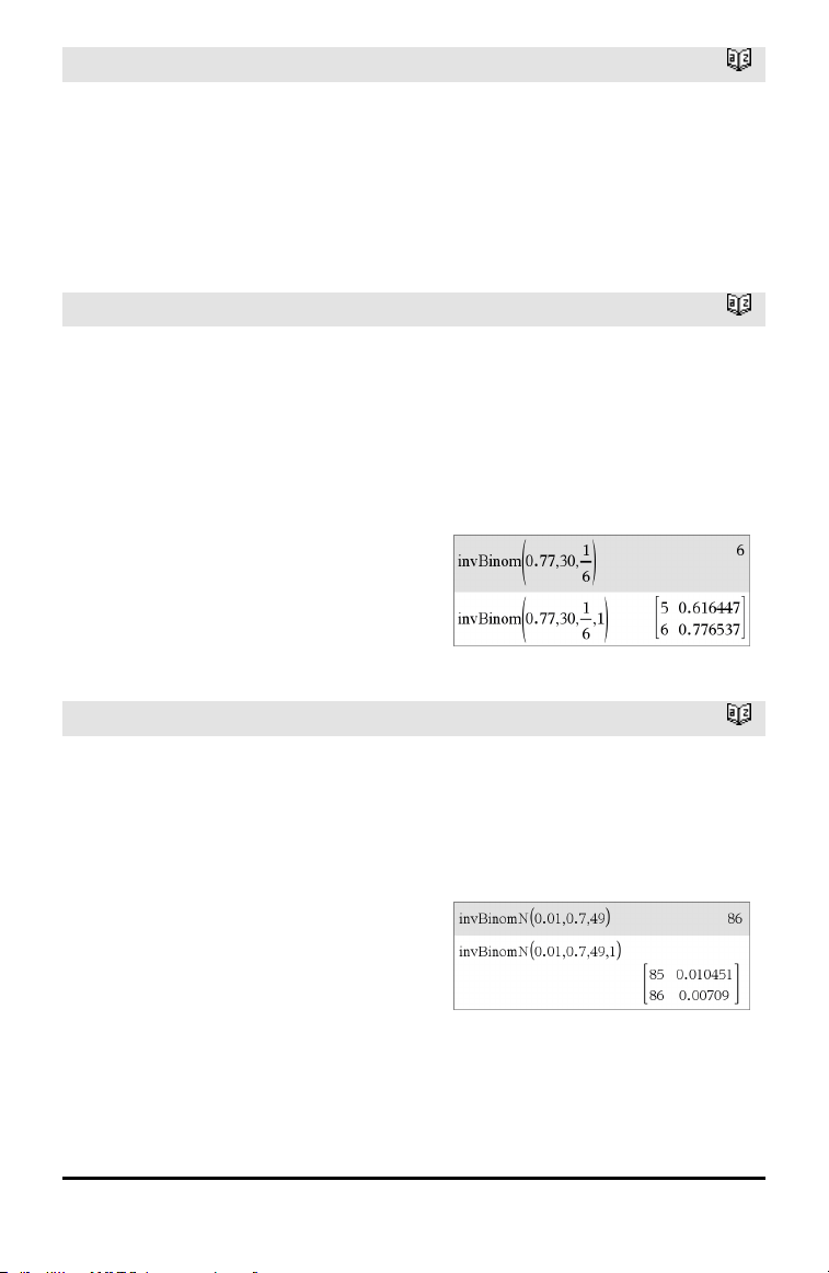
72 Alphabetical Listing
invF()
Catalog >
invF(Area,dfNumer,dfDenom)
invF(Area,dfNumer,dfDenom)
computes the Inverse cumulative F
distribution function specified by dfNumer
and dfDenom for a given Area under the
curve.
invBinom()
Catalog >
invBinom
(CumulativeProb,NumTrials,Prob,
OutputForm)⇒ scalar or matrix
Inverse binomial. Given the number of trials
(NumTrials) and the probability of success
of each trial (Prob), this function returns
the minimum number of successes, k, such
that the value, k, is greater than or equal to
the given cumulative probability
(CumulativeProb).
OutputForm=0, displays result as a scalar
(default).
OutputForm=1, displays result as a matrix.
Example: Mary and Kevin are playing a dice
game. Mary has to guess the maximum
number of times 6 shows up in 30 rolls. If the
number 6 shows upthat many times or less,
Mary wins. Furthermore, the smaller the
number that she guesses, the greater her
winnings. What is the smallest number Mary
can guess if she wants the probability of
winning to be greater than 77%?
invBinomN()
Catalog >
invBinomN(CumulativeProb,Prob,
NumSuccess,OutputForm)⇒ scalar or
matrix
Inverse binomial with respect to N. Given
the probability of success of each trial
(Prob), and the number of successes
(NumSuccess), this function returns the
minimum number of trials, N, such that the
value, N, is less than or equal to the given
cumulative probability (CumulativeProb).
OutputForm=0, displays result as a scalar
(default).
OutputForm=1, displays result as a matrix.
Example: Monique is practicing goal shots
for netball. She knows from experience that
her chance of making any one shot is 70%.
She plans to practice until she scores 50
goals. How many shots must she attempt to
ensure thatthe probability of making at least
50 goals is more than 0.99?
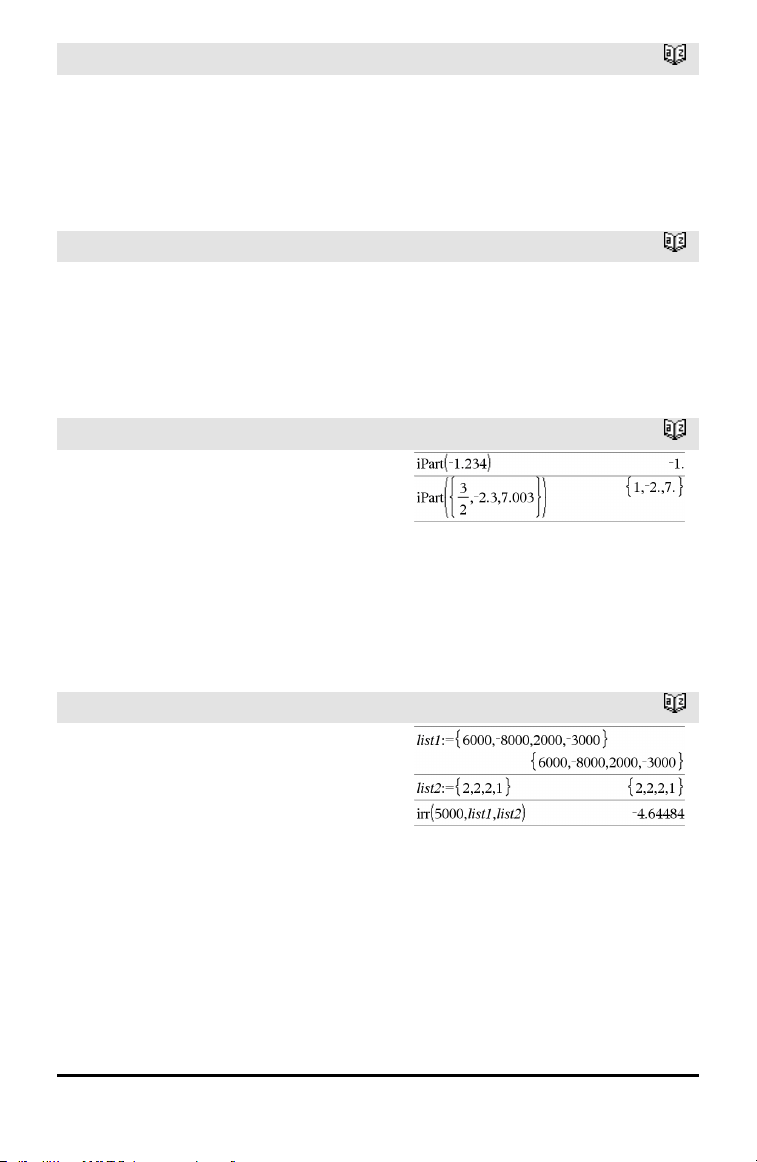
invNorm()
Catalog >
invNorm(Area[,μ[,σ]])
Computes the inverse cumulative normal
distribution function for a given Area under
the normal distribution curve specified by μ
and σ.
invt()
Catalog >
invt(Area,df)
Computes the inverse cumulative student-t
probability function specified by degree of
freedom, df for a given Area under the
curve.
iPart()
Catalog >
iPart(Number) ⇒ integer
iPart(List1) ⇒ list
iPart(Matrix1) ⇒ matrix
Returns the integer part of the argument.
For lists and matrices, returns the integer
part of each element.
The argument can be a real or a complex
number.
irr()
Catalog >
irr(CF0,CFList [,CFFreq]) ⇒ value
Financial function that calculates internal
rate of return of an investment.
CF0 is the initial cash flow at time 0; it
must be a real number.
CFList is a list of cash flow amounts after
the initial cash flow CF0.
Alphabetical Listing 73
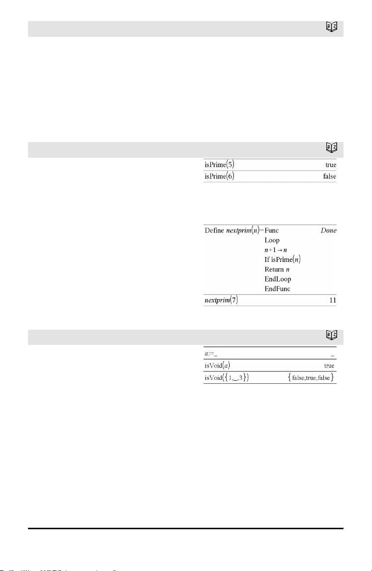
74 Alphabetical Listing
irr()
Catalog >
CFFreq is an optional list in which each
element specifies the frequency of
occurrence for a grouped (consecutive) cash
flow amount, which is the corresponding
element of CFList. The default is 1; if you
enter values, they must be positive integers
< 10,000.
Note: See also mirr(), page 94.
isPrime()
Catalog >
isPrime(Number) ⇒ Boolean constant
expression
Returns true or false to indicate if number
is a whole number ≥2 that is evenly
divisible only by itself and 1.
If Number exceeds about 306 digits and has
no factors ≤1021, isPrime(Number) displays
an error message.
Note for entering the example: For
instructions on entering multi-line program
and function definitions, refer to the
Calculator section of your product
guidebook.
Function to find the next prime after a
specified number:
isVoid()
Catalog >
isVoid(Var) ⇒ Boolean constant
expression
isVoid(Expr) ⇒ Boolean constant
expression
isVoid(List) ⇒ list of Boolean constant
expressions
Returns true or false to indicate if the
argument is a void data type.
For more information on void elements, see
page 196.
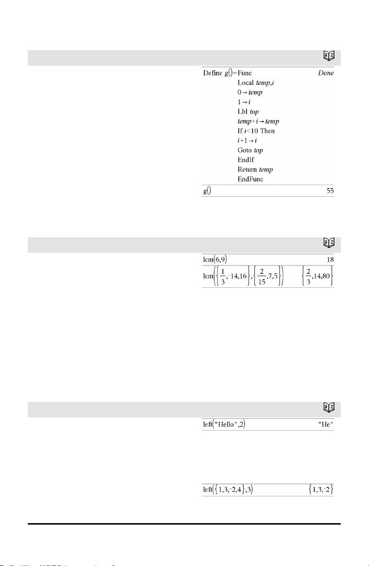
L
Lbl
Catalog >
Lbl labelName
Defines a label with the name labelName
within a function.
You can use a Goto labelName instruction
to transfer control to the instruction
immediately following the label.
labelName must meet the same naming
requirements as a variable name.
Note for entering the example: For
instructions on entering multi-line program
and function definitions, refer to the
Calculator section of your product
guidebook.
lcm()
Catalog >
lcm(Number1, Number2) ⇒ expression
lcm(List1, List2) ⇒ list
lcm(Matrix1, Matrix2) ⇒ matrix
Returns the least common multiple of the
two arguments. The lcm of two fractions is
the lcm of their numerators divided by the
gcd of their denominators. The lcm of
fractional floating-point numbers is their
product.
For two lists or matrices, returns the least
common multiples of the corresponding
elements.
left()
Catalog >
left(sourceString[, Num]) ⇒ string
Returns the leftmost Num characters
contained in character string sourceString.
If you omit Num, returns all of
sourceString.
left(List1[, Num]) ⇒ list
Alphabetical Listing 75
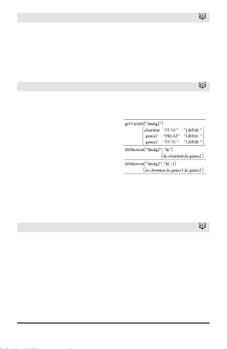
76 Alphabetical Listing
left()
Catalog >
Returns the leftmost Num elements
contained in List1.
If you omit Num, returns all of List1.
left(Comparison) ⇒ expression
Returns the left-hand side of an equation or
inequality.
libShortcut()
Catalog >
libShortcut(LibNameString,
ShortcutNameString
[, LibPrivFlag]) ⇒ list of variables
Creates a variable group in the current
problem that contains references to all the
objects in the specified library document
libNameString. Also adds the group
members to the Variables menu. You can
then refer to each object using its
ShortcutNameString.
Set LibPrivFlag=0 to exclude private
library objects (default)
Set LibPrivFlag=1 to include private
library objects
To copy a variable group, see CopyVar on
page 24.
To delete a variable group, see DelVar on
page 38.
This example assumes a properly stored and
refreshed library document named linalg2
that contains objects defined as clearmat,
gauss1, and gauss2.
LinRegBx
Catalog >
LinRegBx X,Y[,[Freq][,Category,Include]]
Computes the linear regression y = a+b•x on
lists X and Y with frequency Freq. A
summary of results is stored in the
stat.results variable. (See page 145.)
All the lists must have equal dimension
except for Include.
X and Y are lists of independent and
dependent variables.

LinRegBx
Catalog >
Freq is an optional list of frequency values.
Each element in Freq specifies the
frequency of occurrence for each
corresponding X and Y data point. The
default value is 1. All elements must be
integers ≥ 0.
Category is a list of numeric or string
category codes for the corresponding X and
Y data.
Include is a list of one or more of the
category codes. Only those data items
whose category code is included in this list
are included in the calculation.
For information on the effect of empty
elements in a list, see “Empty (Void)
Elements,” page 196.
Output
variable
Description
stat.RegEqn
Regression Equation: a+b•x
stat.a, stat.b Regression coefficients
stat.r
2
Coefficientof determination
stat.r Correlation coefficient
stat.Resid Residuals from the regression
stat.XReg
Listof data points in the modifiedX List actually used in the regression based on
restrictions of Freq, Category List, and Include Categories
stat.YReg
Listof data points in the modifiedY List actually used inthe regression basedon
restrictions of Freq, Category List, and Include Categories
stat.FreqReg
Listof frequencies corresponding to stat.XReg and stat.YReg
LinRegMx
Catalog >
LinRegMx X,Y[,[Freq][,Category,Include]]
Computes the linear regression y = m•x+b on
lists X and Y with frequency Freq. A
summary of results is stored in the
stat.results variable. (See page 145.)
All the lists must have equal dimension
except for Include.
Alphabetical Listing 77

78 Alphabetical Listing
LinRegMx
Catalog >
X and Y are lists of independent and
dependent variables.
Freq is an optional list of frequency values.
Each element in Freq specifies the
frequency of occurrence for each
corresponding X and Y data point. The
default value is 1. All elements must be
integers ≥ 0.
Category is a list of numeric or string
category codes for the corresponding X and
Y data.
Include is a list of one or more of the
category codes. Only those data items
whose category code is included in this list
are included in the calculation.
For information on the effect of empty
elements in a list, see “Empty (Void)
Elements,” page 196.
Output
variable
Description
stat.RegEqn
Regression Equation: y = m•x+b
stat.m,
stat.b
Regression coefficients
stat.r
2
Coefficientof determination
stat.r Correlation coefficient
stat.Resid Residuals from the regression
stat.XReg
Listof data points in the modifiedX List actually used in the regression based on
restrictions of Freq, Category List, and Include Categories
stat.YReg
Listof data points in the modifiedY List actually used inthe regression basedon
restrictions of Freq, Category List, and Include Categories
stat.FreqReg
Listof frequencies corresponding to stat.XReg and stat.YReg
LinRegtIntervals
Catalog >
LinRegtIntervals X,Y[,F[,0[,CLev]]]
For Slope. Computes a level C confidence
interval for the slope.

LinRegtIntervals
Catalog >
LinRegtIntervals X,Y[,F[,1,Xval[,CLev]]]
For Response. Computes a predicted y-value,
a level C prediction interval for a single
observation, and a level C confidence
interval for the mean response.
A summary of results is stored in the
stat.results variable. (See page 145.)
All the lists must have equal dimension.
X and Y are lists of independent and
dependent variables.
F is an optional list of frequency values.
Each element in F specifies the frequency of
occurrence for each corresponding X and Y
data point. The default value is 1. All
elements must be integers ≥ 0.
For information on the effect of empty
elements in a list, see “Empty (Void)
Elements,” page 196.
Output variable Description
stat.RegEqn
Regression Equation: a+b•x
stat.a, stat.b Regression coefficients
stat.df Degrees of freedom
stat.r
2
Coefficientof determination
stat.r Correlation coefficient
stat.Resid Residuals from the regression
For Slope type only
Output variable Description
[stat.CLower, stat.CUpper] Confidence interval for the slope
stat.ME Confidence interval margin of error
stat.SESlope Standard error of slope
stat.s Standard error about the line
For Response type only
Alphabetical Listing 79

80 Alphabetical Listing
Output variable Description
[stat.CLower, stat.CUpper] Confidence interval for the mean response
stat.ME Confidence interval marginof error
stat.SE Standard error of mean response
[stat.LowerPred,
stat.UpperPred]
Prediction interval for a single observation
stat.MEPred Prediction interval marginof error
stat.SEPred Standard error for prediction
stat.y
a + b•XVal
LinRegtTest
Catalog >
LinRegtTest X,Y[,Freq[,Hypoth]]
Computes a linear regression on the X and Y
lists and a t test on the value of slope β and
the correlation coefficient ρ for the equation
y=α+βx. It tests the null hypothesis H
0
:β=0
(equivalently, ρ=0) against one of three
alternative hypotheses.
All the lists must have equal dimension.
X and Y are lists of independent and
dependent variables.
Freq is an optional list of frequency values.
Each element in Freq specifies the
frequency of occurrence for each
corresponding X and Y data point. The
default value is 1. All elements must be
integers ≥ 0.
Hypoth is an optional value specifying one
of three alternative hypotheses against
which the null hypothesis (H
0
:β=ρ=0) will be
tested.
For H
a
: β≠0 and ρ≠0 (default), set Hypoth=0
For H
a
: β<0 and ρ<0, set Hypoth<0
For H
a
: β>0 and ρ>0, set Hypoth>0
A summary of results is stored in the
stat.results variable. (See page 145.)
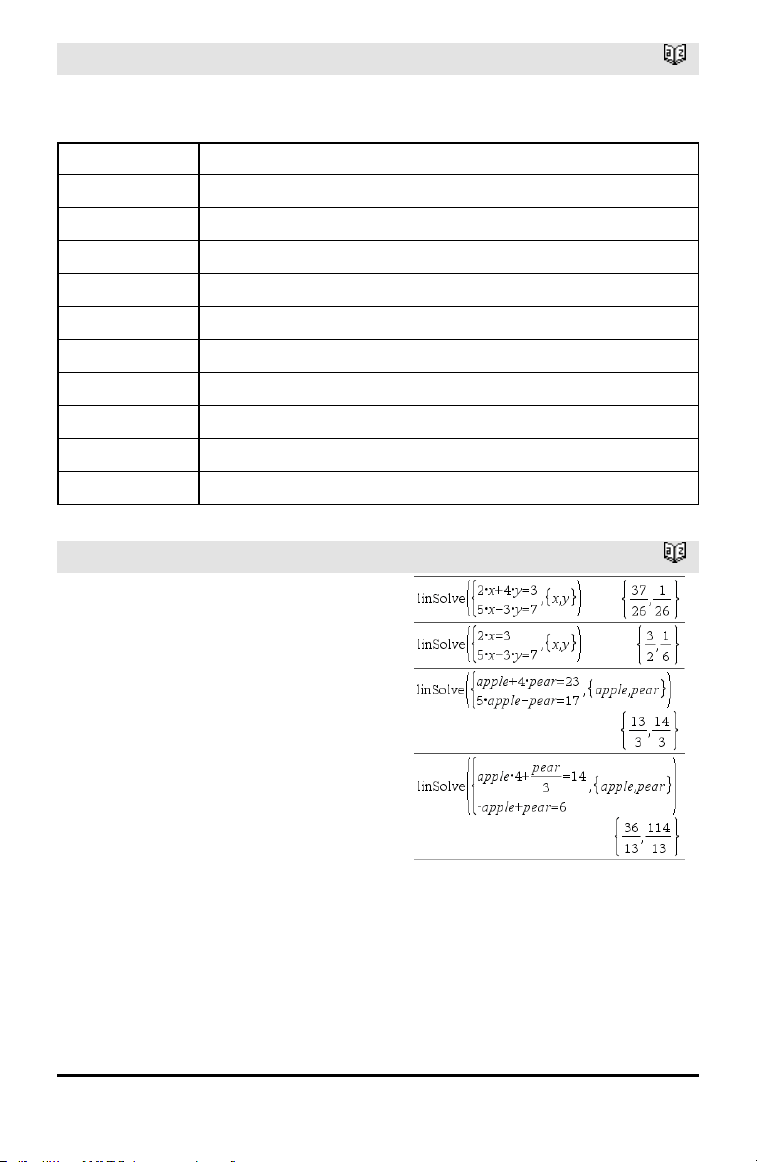
LinRegtTest
Catalog >
For information on the effect of empty
elements in a list, see “Empty (Void)
Elements,” page 196.
Output variable Description
stat.RegEqn
Regression equation: a + b•x
stat.t
t-Statistic for significance test
stat.PVal Smallest level of significance at whichthe null hypothesis can be rejected
stat.df Degrees of freedom
stat.a, stat.b Regression coefficients
stat.s Standard error about the line
stat.SESlope Standard error of slope
stat.r
2
Coefficientof determination
stat.r Correlation coefficient
stat.Resid Residuals from the regression
linSolve()
Catalog >
linSolve(SystemOfLinearEqns, Var1,
Var2, ...) ⇒ list
linSolve(LinearEqn1 and LinearEqn2 and
..., Var1, Var2, ...) ⇒ list
linSolve({LinearEqn1, LinearEqn2, ...},
Var1, Var2, ...) ⇒ list
linSolve(SystemOfLinearEqns, {Var1,
Var2, ...}) ⇒ list
linSolve(LinearEqn1 and LinearEqn2 and
..., {Var1, Var2, ...}) ⇒ list
linSolve({LinearEqn1, LinearEgn2, ...},
{Var1, Var2, ...}) ⇒ list
Returns a list of solutions for the variables
Var1, Var2, ...
Alphabetical Listing 81
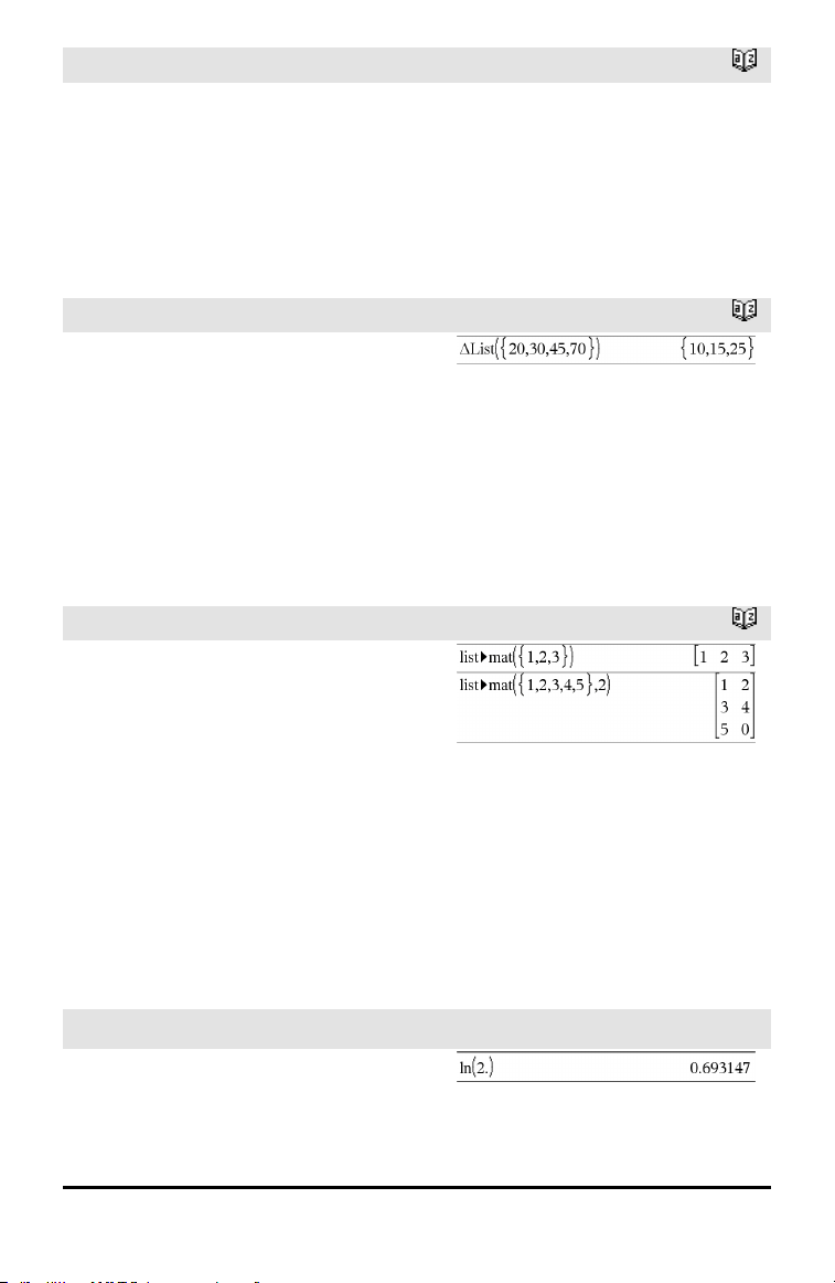
82 Alphabetical Listing
linSolve()
Catalog >
The first argument must evaluate to a
system of linear equations or a single linear
equation. Otherwise, an argument error
occurs.
For example, evaluating linSolve(x=1
and x=2,x) produces an “Argument
Error” result.
ΔList()
Catalog >
ΔList(List1) ⇒ list
Note: You can insert this function from the
keyboard by typing deltaList(...).
Returns a list containing the differences
between consecutive elements in List1.
Each element of List1 is subtracted from
the next element of List1. The resulting list
is always one element shorter than the
original List1.
list►mat()
Catalog >
list►mat(List [, elementsPerRow]) ⇒
matrix
Returns a matrix filled row-by-row with the
elements from List.
elementsPerRow, if included, specifies the
number of elements per row. Default is the
number of elements in List (one row).
If List does not fill the resulting matrix,
zeros are added.
Note: You can insert this function from the
computer keyboard by typing list@>mat
(...).
ln()
/u keys
ln(Value1) ⇒ value
ln(List1) ⇒ list

ln()
/u keys
Returns the natural logarithm of the
argument.
For a list, returns the natural logarithms of
the elements.
If complex formatmode is Real:
If complex formatmode is Rectangular:
ln(squareMatrix1) ⇒ squareMatrix
Returns the matrix natural logarithm of
squareMatrix1. This is not the same as
calculating the natural logarithm of each
element. For information about the
calculation method, refer to cos() on.
squareMatrix1 must be diagonalizable. The
result always contains floating-point
numbers.
In Radian angle mode and Rectangular
complex format:
To see the entire result, press £ and then
use ¡and¢ to move the cursor.
LnReg
Catalog >
LnReg X, Y[, [Freq] [, Category, Include]]
Computes the logarithmic regression y =
a+b•ln(x) on lists X and Y with frequency
Freq. A summary of results is stored in the
stat.results variable. (See page 145.)
All the lists must have equal dimension
except for Include.
X and Y are lists of independent and
dependent variables.
Freq is an optional list of frequency values.
Each element in Freq specifies the
frequency of occurrence for each
corresponding X and Y data point. The
default value is 1. All elements must be
integers ≥ 0.
Alphabetical Listing 83

84 Alphabetical Listing
LnReg
Catalog >
Category is a list of numeric or string
category codes for the corresponding X and
Y data.
Include is a list of one or more of the
category codes. Only those data items
whose category code is included in this list
are included in the calculation.
For information on the effect of empty
elements in a list, see “Empty (Void)
Elements,” page 196.
Output
variable
Description
stat.RegEqn
Regression equation: a+b•ln(x)
stat.a, stat.b Regression coefficients
stat.r
2
Coefficientof linear determination for transformeddata
stat.r Correlation coefficient for transformed data (ln(x), y)
stat.Resid Residuals associated with the logarithmicmodel
stat.ResidTrans Residuals associated with linear fitof transformed data
stat.XReg
Listof data points in the modifiedX List actually used in the regression based on
restrictions of Freq, Category List, and Include Categories
stat.YReg
Listof data points in the modifiedY List actually used inthe regression basedon
restrictions of Freq, Category List, and Include Categories
stat.FreqReg
Listof frequencies corresponding to stat.XReg and stat.YReg
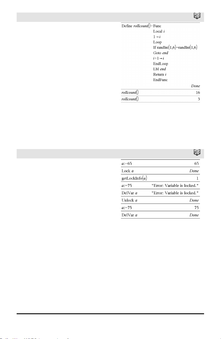
Local
Catalog >
Local Var1[, Var2] [, Var3] ...
Declares the specified vars as local
variables. Those variables exist only during
evaluation of a function and are deleted
when the function finishes execution.
Note: Local variables save memory because
they only exist temporarily. Also, they do
not disturb any existing global variable
values. Local variables must be used for For
loops and for temporarily saving values in a
multi-line function since modifications on
global variables are not allowed in a
function.
Note for entering the example: For
instructions on entering multi-line program
and function definitions, refer to the
Calculator section of your product
guidebook.
Lock
Catalog >
LockVar1[, Var2] [, Var3] ...
LockVar.
Locks the specified variables or variable
group. Locked variables cannot be modified
or deleted.
You cannot lock or unlock the system
variable Ans, and you cannot lock the
system variable groups stat. or tvm.
Note: The Lock command clears the
Undo/Redo history when applied to
unlocked variables.
See unLock, page 163, and getLockInfo(),
page 63.
Alphabetical Listing 85
86 Alphabetical Listing
log()
/s keys
log(Value1[,Value2]) ⇒ value
log(List1[,Value2]) ⇒ list
Returns the base-Value2 logarithm of the
first argument.
Note: See also Log template, page 2.
For a list, returns the base-Value2
logarithm of the elements.
If the second argument is omitted, 10 is
used as the base.
If complex formatmode is Real:
If complex formatmode is Rectangular:
log(squareMatrix1[,Value]) ⇒
squareMatrix
Returns the matrix base-Value logarithm of
squareMatrix1. This is not the same as
calculating the base-Value logarithm of
each element. For information about the
calculation method, refer to cos().
squareMatrix1 must be diagonalizable. The
result always contains floating-point
numbers.
If the base argument is omitted, 10 is used
as base.
In Radian angle mode and Rectangular
complex format:
To see the entire result, press £ and then
use ¡and¢ to move the cursor.
Logistic
Catalog >
Logistic X, Y[, [Freq] [, Category, Include]]
Computes the logistic regression y = (c/
(1+a•e
-bx
)) on lists X and Y with frequency
Freq. A summary of results is stored in the
stat.results variable. (See page 145.)
All the lists must have equal dimension
except for Include.

Logistic
Catalog >
X and Y are lists of independent and
dependent variables.
Freq is an optional list of frequency values.
Each element in Freq specifies the
frequency of occurrence for each
corresponding X and Y data point. The
default value is 1. All elements must be
integers ≥ 0.
Category is a list of numeric or string
category codes for the corresponding X and
Y data.
Include is a list of one or more of the
category codes. Only those data items
whose category code is included in this list
are included in the calculation.
For information on the effect of empty
elements in a list, see “Empty (Void)
Elements,” page 196.
Output
variable
Description
stat.RegEqn
Regression equation: c/(1+a•e
-bx
)
stat.a,
stat.b, stat.c
Regression coefficients
stat.Resid Residuals from the regression
stat.XReg
Listof data points in the modifiedX List actually used in the regression based on
restrictions of Freq, Category List, and Include Categories
stat.YReg
Listof data points in the modifiedY List actually used inthe regression basedon
restrictions of Freq, Category List, and Include Categories
stat.FreqReg
Listof frequencies corresponding to stat.XReg and stat.YReg
LogisticD
Catalog >
LogisticD X, Y [, [Iterations] , [Freq] [,
Category, Include] ]
Computes the logistic regression y = (c/
(1+a•e
-bx
)+d) on lists X and Y with frequency
Freq, using a specified number of
Iterations. A summary of results is stored in
the stat.results variable. (See page 145.)
Alphabetical Listing 87

88 Alphabetical Listing
LogisticD
Catalog >
All the lists must have equal dimension
except for Include.
X and Y are lists of independent and
dependent variables.
Freq is an optional list of frequency values.
Each element in Freq specifies the
frequency of occurrence for each
corresponding X and Y data point. The
default value is 1. All elements must be
integers ≥ 0.
Category is a list of numeric or string
category codes for the corresponding X and
Y data.
Include is a list of one or more of the
category codes. Only those data items
whose category code is included in this list
are included in the calculation.
For information on the effect of empty
elements in a list, see “Empty (Void)
Elements,” page 196.
Output
variable
Description
stat.RegEqn
Regression equation: c/(1+a•e
-bx
)+d)
stat.a, stat.b,
stat.c, stat.d
Regression coefficients
stat.Resid Residuals from the regression
stat.XReg
Listof data points in the modifiedX List actually used in the regression based on
restrictions of Freq, Category List, and Include Categories
stat.YReg
Listof data points in the modifiedY List actually used inthe regression basedon
restrictions of Freq, Category List, and Include Categories
stat.FreqReg
Listof frequencies corresponding to stat.XReg and stat.YReg
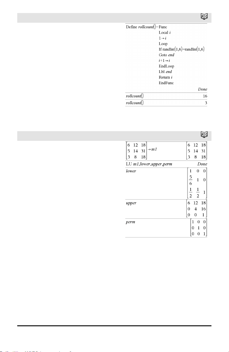
Loop
Catalog >
Loop
Block
EndLoop
Repeatedly executes the statements in
Block. Note that the loop will be executed
endlessly, unless a Goto or Exit instruction
is executed within Block.
Block is a sequence of statements
separated with the “:” character.
Note for entering the example: For
instructions on entering multi-line program
and function definitions, refer to the
Calculator section of your product
guidebook.
LU
Catalog >
LU Matrix, lMatrix, uMatrix, pMatrix
[,Tol]
Calculates the Doolittle LU (lower-upper)
decomposition of a real or complex matrix.
The lower triangular matrix is stored in
lMatrix, the upper triangular matrix in
uMatrix, and the permutation matrix
(which describes the row swaps done
during the calculation) in pMatrix.
lMatrix•uMatrix = pMatrix•matrix
Optionally, any matrix element is treated as
zero if its absolute value is less than Tol.
This tolerance is used only if the matrix has
floating-point entries and does not contain
any symbolic variables that have not been
assigned a value. Otherwise, Tol is ignored.
• If you use /· or set the Auto or
Approximate mode to Approximate,
computations are done using floating-
point arithmetic.
• If Tol is omitted or not used, the default
tolerance is calculated as:
5E⁻14•max(dim(Matrix))•rowNorm
(Matrix)
Alphabetical Listing 89
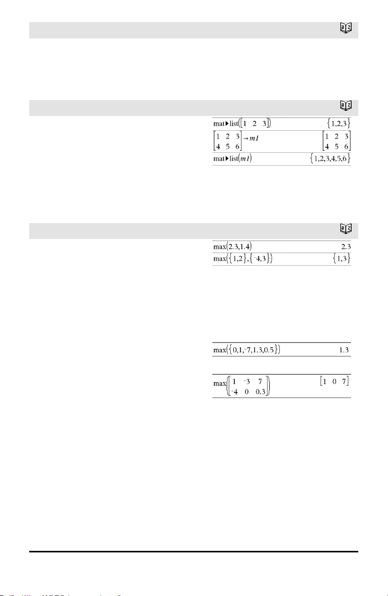
90 Alphabetical Listing
LU
Catalog >
The LU factorization algorithm uses partial
pivoting with row interchanges.
M
mat►list()
Catalog >
mat►list(Matrix) ⇒ list
Returns a list filled with the elements in
Matrix. The elements are copied from
Matrix row by row.
Note: You can insert this function from the
computer keyboard by typing mat@>list
(...).
max()
Catalog >
max(Value1, Value2) ⇒ expression
max(List1, List2) ⇒ list
max(Matrix1, Matrix2) ⇒ matrix
Returns the maximum of the two
arguments. If the arguments are two lists
or matrices, returns a list or matrix
containing the maximum value of each pair
of corresponding elements.
max(List) ⇒ expression
Returns the maximum element in list.
max(Matrix1) ⇒ matrix
Returns a row vector containing the
maximum element of each column in
Matrix1.
Empty (void) elements are ignored. For
more information on empty elements, see
page 196.
Note: See also min().
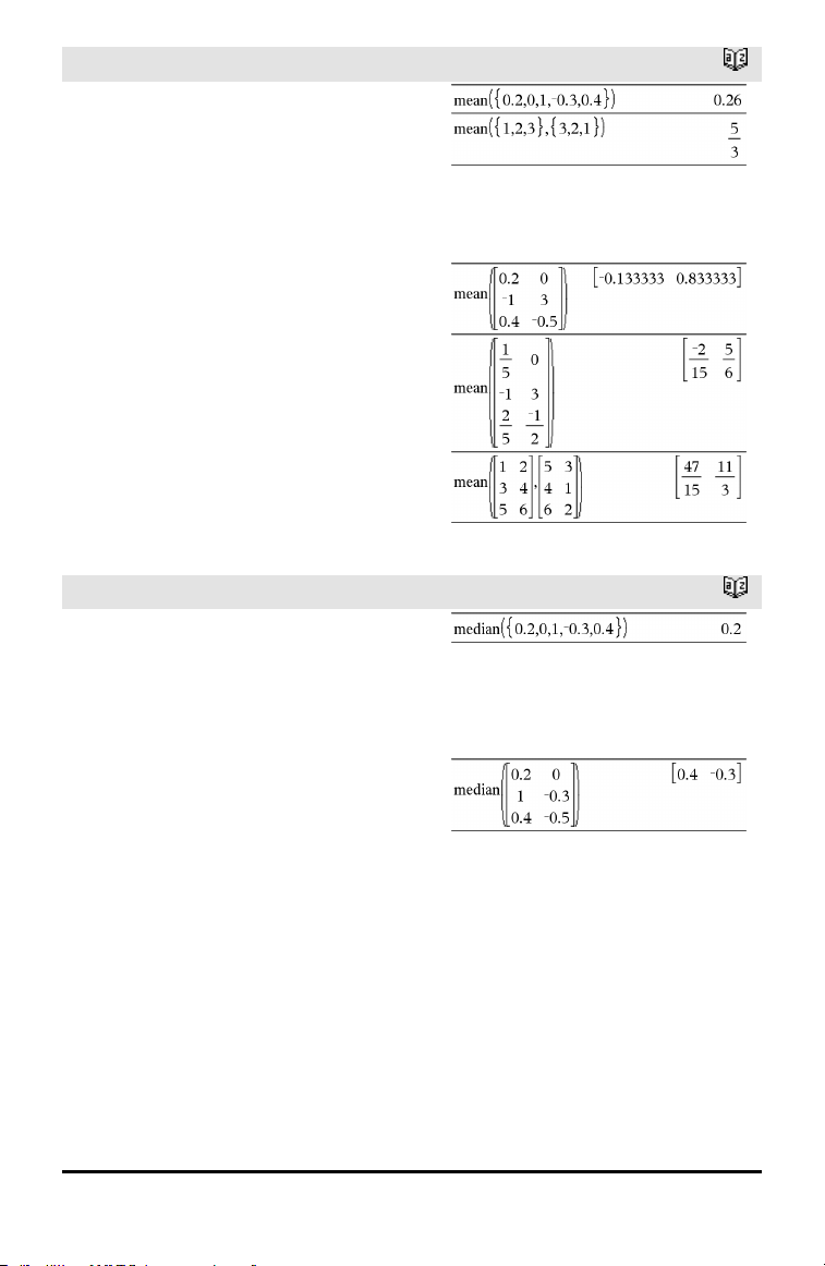
mean()
Catalog >
mean(List[, freqList]) ⇒ expression
Returns the mean of the elements in List.
Each freqList element counts the number
of consecutive occurrences of the
corresponding element in List.
mean(Matrix1[, freqMatrix]) ⇒ matrix
Returns a row vector of the means of all
the columns in Matrix1.
Each freqMatrix element counts the
number of consecutive occurrences of the
corresponding element in Matrix1.
Empty (void) elements are ignored. For
more information on empty elements, see
page 196.
In Rectangular vector format:
median()
Catalog >
median(List[, freqList]) ⇒ expression
Returns the median of the elements in List.
Each freqList element counts the number
of consecutive occurrences of the
corresponding element in List.
median(Matrix1[, freqMatrix]) ⇒ matrix
Returns a row vector containing the
medians of the columns in Matrix1.
Each freqMatrix element counts the
number of consecutive occurrences of the
corresponding element in Matrix1.
Notes:
• All entries in the list or matrix must
simplify to numbers.
• Empty (void) elements in the list or
matrix are ignored. For more information
on empty elements, see page 196.
Alphabetical Listing 91

92 Alphabetical Listing
MedMed
Catalog >
MedMed X,Y [, Freq] [, Category, Include]]
Computes the median-median line y =
(m•x+b) on lists X and Y with frequency
Freq. A summary of results is stored in the
stat.results variable. (See page 145.)
All the lists must have equal dimension
except for Include.
X and Y are lists of independent and
dependent variables.
Freq is an optional list of frequency values.
Each element in Freq specifies the
frequency of occurrence for each
corresponding X and Y data point. The
default value is 1. All elements must be
integers ≥ 0.
Category is a list of numeric or string
category codes for the corresponding X and
Y data.
Include is a list of one or more of the
category codes. Only those data items
whose category code is included in this list
are included in the calculation.
For information on the effect of empty
elements in a list, see “Empty (Void)
Elements,” page 196.
Output
variable
Description
stat.RegEqn
Median-median line equation: m•x+b
stat.m,
stat.b
Model coefficients
stat.Resid Residuals from the median-median line
stat.XReg
Listof data points in the modifiedX List actually used in the regression based on
restrictions of Freq, Category List, and Include Categories
stat.YReg
Listof data points in the modifiedY List actually used inthe regression basedon
restrictions of Freq, Category List, and Include Categories
stat.FreqReg
Listof frequencies corresponding to stat.XReg and stat.YReg
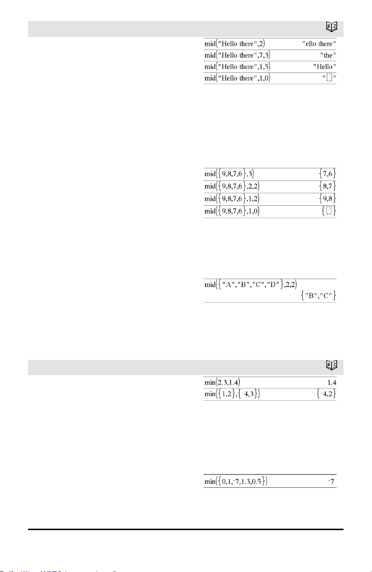
mid()
Catalog >
mid(sourceString, Start[, Count]) ⇒
string
Returns Count characters from character
string sourceString, beginning with
character number Start.
If Count is omitted or is greater than the
dimension of sourceString, returns all
characters from sourceString, beginning
with character number Start.
Count must be ≥ 0. If Count = 0, returns an
empty string.
mid(sourceList, Start [, Count]) ⇒ list
Returns Count elements from sourceList,
beginning with element number Start.
If Count is omitted or is greater than the
dimension of sourceList, returns all
elements from sourceList, beginning with
element number Start.
Count must be ≥ 0. If Count = 0, returns an
empty list.
mid(sourceStringList, Start[, Count]) ⇒
list
Returns Count strings from the list of
strings sourceStringList, beginning with
element number Start.
min()
Catalog >
min(Value1, Value2) ⇒ expression
min(List1, List2) ⇒ list
min(Matrix1, Matrix2) ⇒ matrix
Returns the minimum of the two
arguments. If the arguments are two lists
or matrices, returns a list or matrix
containing the minimum value of each pair
of corresponding elements.
min(List) ⇒ expression
Returns the minimum element of List.
Alphabetical Listing 93
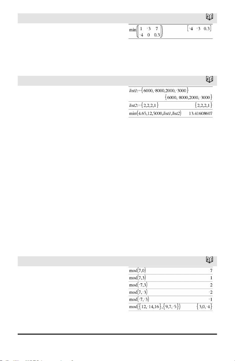
94 Alphabetical Listing
min()
Catalog >
min(Matrix1) ⇒ matrix
Returns a row vector containing the
minimum element of each column in
Matrix1.
Note: See also max().
mirr()
Catalog >
mirr
(financeRate,reinvestRate,CF0,CFList
[,CFFreq])
Financial function that returns the modified
internal rate of return of an investment.
financeRate is the interest rate that you
pay on the cash flow amounts.
reinvestRate is the interest rate at which
the cash flows are reinvested.
CF0 is the initial cash flow at time 0; it
must be a real number.
CFList is a list of cash flow amounts after
the initial cash flow CF0.
CFFreq is an optional list in which each
element specifies the frequency of
occurrence for a grouped (consecutive) cash
flow amount, which is the corresponding
element of CFList. The default is 1; if you
enter values, they must be positive integers
< 10,000.
Note: See also irr(), page 73.
mod()
Catalog >
mod(Value1, Value2) ⇒ expression
mod(List1, List2) ⇒ list
mod(Matrix1, Matrix2) ⇒ matrix
Returns the first argument modulo the
second argument as defined by the
identities:
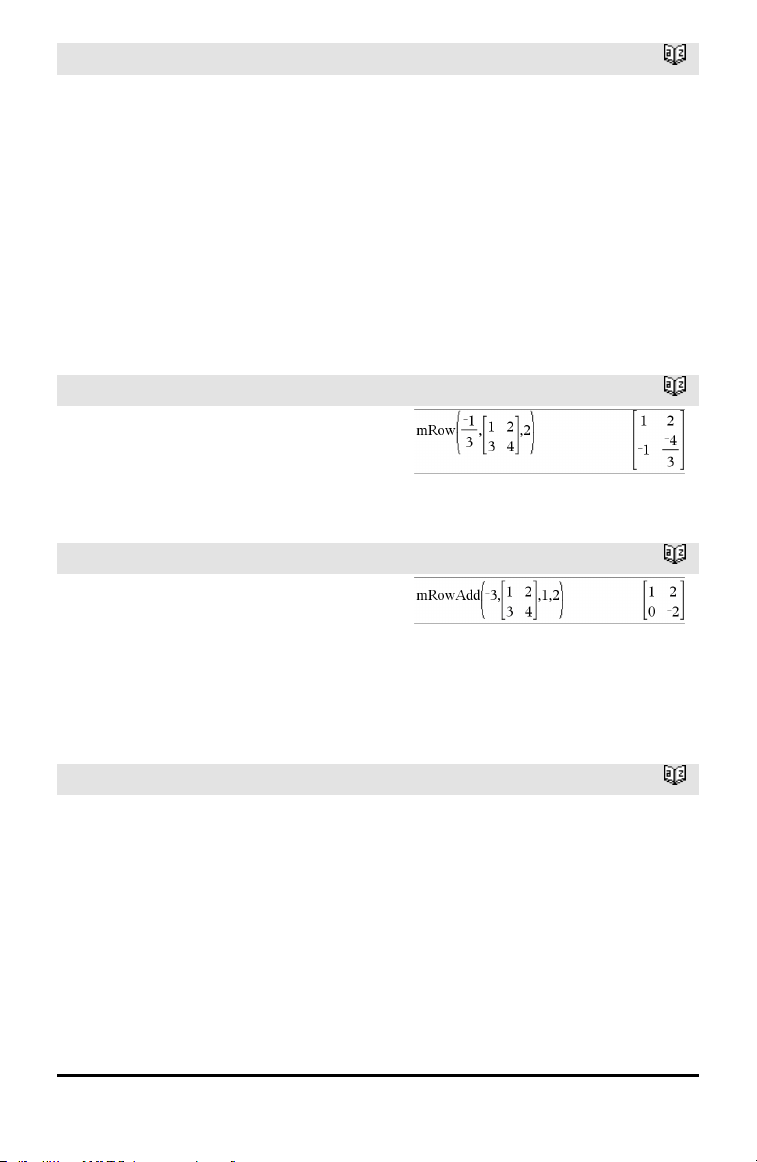
mod()
Catalog >
mod(x,0) = x
mod(x,y) = x − y floor(x/y)
When the second argument is non-zero, the
result is periodic in that argument. The
result is either zero or has the same sign as
the second argument.
If the arguments are two lists or two
matrices, returns a list or matrix containing
the modulo of each pair of corresponding
elements.
Note: See also remain(), page 124
mRow()
Catalog >
mRow(Value, Matrix1, Index) ⇒ matrix
Returns a copy of Matrix1 with each
element in row Index of Matrix1 multiplied
by Value.
mRowAdd()
Catalog >
mRowAdd(Value, Matrix1, Index1, Index2)
⇒ matrix
Returns a copy of Matrix1 with each
element in row Index2 of Matrix1 replaced
with:
Value • row Index1 + row Index2
MultReg
Catalog >
MultReg Y, X1[,X2[,X3,…[,X10]]]
Calculates multiple linear regression of list Y
on lists X1, X2, …, X10. A summary of
results is stored in the stat.results variable.
(See page 145.)
All the lists must have equal dimension.
For information on the effect of empty
elements in a list, see “Empty (Void)
Elements,” page 196.
Alphabetical Listing 95

96 Alphabetical Listing
Output variable Description
stat.RegEqn
Regression Equation: b0+b1•x1+b2•x2+ ...
stat.b0, stat.b1, ... Regression coefficients
stat.R
2
Coefficientof multiple determination
stat.yList yList= b0+b1•x1+ ...
stat.Resid Residuals from the regression
MultRegIntervals
Catalog >
MultRegIntervals Y, X1[, X2[, X3,…[,
X10]]], XValList[, CLevel]
Computes a predicted y-value, a level C
prediction interval for a single observation,
and a level C confidence interval for the
mean response.
A summary of results is stored in the
stat.results variable. (See page 145.)
All the lists must have equal dimension.
For information on the effect of empty
elements in a list, see “Empty (Void)
Elements,” page 196.
Output variable Description
stat.RegEqn
Regression Equation: b0+b1•x1+b2•x2+ ...
stat.y A point estimate: y = b0 + b1 • xl + ... for XValList
stat.dfError Error degrees of freedom
stat.CLower, stat.CUpper Confidence interval for a mean response
stat.ME Confidence interval marginof error
stat.SE Standard error of mean response
stat.LowerPred,
stat.UpperrPred
Prediction interval for a single observation
stat.MEPred Prediction interval marginof error
stat.SEPred Standard error for prediction
stat.bList Listof regression coefficients, {b0,b1,b2,...}
stat.Resid Residuals from the regression

MultRegTests
Catalog >
MultRegTests Y, X1[, X2[, X3,…[, X10]]]
Multiple linear regression test computes a
multiple linear regression on the given data
and provides the global F test statistic and t
test statistics for the coefficients.
A summary of results is stored in the
stat.results variable. (See page 145.)
For information on the effect of empty
elements in a list, see “Empty (Void)
Elements,” page 196.
Outputs
Output
variable
Description
stat.RegEqn
Regression Equation: b0+b1•x1+b2•x2+ ...
stat.F
Global F test statistic
stat.PVal
P-value associatedwith global F statistic
stat.R
2
Coefficientof multiple determination
stat.AdjR
2
Adjusted coefficient of multiple determination
stat.s Standard deviation of the error
stat.DW Durbin-Watson statistic; used to determine whether first-order auto correlation is
present inthe model
stat.dfReg Regression degrees of freedom
stat.SSReg Regression sum of squares
stat.MSReg Regression mean square
stat.dfError Error degrees of freedom
stat.SSError Error sum of squares
stat.MSError Error meansquare
stat.bList {b0,b1,...} List of coefficients
stat.tList Listof t statistics, one for each coefficient inthe bList
stat.PList ListP-values for each t statistic
stat.SEList List of standard errors for coefficients in bList
stat.yList yList= b0+b1•x1+...
Alphabetical Listing 97
98 Alphabetical Listing
Output
variable
Description
stat.Resid Residuals from the regression
stat.sResid Standardized residuals; obtainedby dividing a residual by its standard deviation
stat.CookDist Cook’s distance; measure of the influence of an observation basedon the residual
and leverage
stat.Leverage Measure of how far the values of the independent variable are from their mean
values
N
nand
/= keys
BooleanExpr1 nand BooleanExpr2 returns
Boolean expression
BooleanList1 nand BooleanList2 returns
Boolean list
BooleanMatrix1 nand BooleanMatrix2
returns Boolean matrix
Returns the negation of a logical and
operation on the two arguments. Returns
true, false, or a simplified form of the
equation.
For lists and matrices, returns comparisons
element by element.
Integer1 nand Integer2 ⇒ integer
Compares two real integers bit-by-bit using
a nand operation. Internally, both integers
are converted to signed, 64-bit binary
numbers. When corresponding bits are
compared, the result is 1 if both bits are 1;
otherwise, the result is 0. The returned
value represents the bit results, and is
displayed according to the Base mode.
You can enter the integers in any number
base. For a binary or hexadecimal entry, you
must use the 0b or 0h prefix, respectively.
Without a prefix, integers are treated as
decimal (base10).
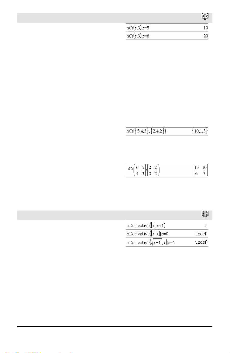
nCr()
Catalog >
nCr(Value1, Value2) ⇒ expression
For integer Value1 and Value2 with
Value1 ≥ Value2≥ 0, nCr() is the number of
combinations of Value1 things taken
Value2 at a time. (This is also known as a
binomial coefficient.)
nCr(Value, 0) ⇒ 1
nCr(Value, negInteger) ⇒ 0
nCr(Value, posInteger) ⇒ Value•
(Value−1) ... (Value−posInteger+1)/
posInteger!
nCr(Value, nonInteger) ⇒ expression! /
((Value−nonInteger)!•nonInteger!)
nCr(List1, List2) ⇒ list
Returns a list of combinations based on the
corresponding element pairs in the two
lists. The arguments must be the same size
list.
nCr(Matrix1, Matrix2) ⇒ matrix
Returns a matrix of combinations based on
the corresponding element pairs in the two
matrices. The arguments must be the same
size matrix.
nDerivative()
Catalog >
nDerivative(Expr1,Var=Value[,Order])
⇒ value
nDerivative(Expr1,Var[,Order])
|Var=Value ⇒ value
Returns the numerical derivative calculated
using auto differentiation methods.
When Value is specified, it overrides any
prior variable assignment or any current “|”
substitution for the variable.
If the variable Var does not contain a
numeric value, you must provide Value.
Order of the derivative must be 1 or 2.
Alphabetical Listing 99
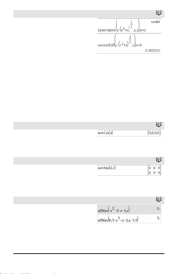
100 Alphabetical Listing
nDerivative()
Catalog >
Note: The nDerivative() algorithm has a
limitiation: it works recursively through the
unsimplified expression, computing the
numeric value of the first derivative (and
second, if applicable) and the evaluation of
each subexpression, which may lead to an
unexpected result.
Consider the example on the right. The first
derivative of x•(x^2+x)^(1/3) at x=0 is equal
to 0. However, because the first derivative
of the subexpression (x^2+x)^(1/3) is
undefined at x=0, and this value is used to
calculate the derivative of the total
expression, nDerivative() reports the result
as undefined and displays a warning
message.
If you encounter this limitation, verify the
solution graphically. You can also try using
centralDiff().
newList()
Catalog >
newList(numElements) ⇒ list
Returns a list with a dimension of
numElements. Each element is zero.
newMat()
Catalog >
newMat(numRows, numColumns) ⇒
matrix
Returns a matrix of zeros with the
dimension numRows by numColumns.
nfMax()
Catalog >
nfMax(Expr, Var) ⇒ value
nfMax(Expr, Var, lowBound) ⇒ value
nfMax(Expr, Var, lowBound, upBound) ⇒
value
nfMax(Expr, Var) |
lowBound≤Var≤upBound ⇒ value
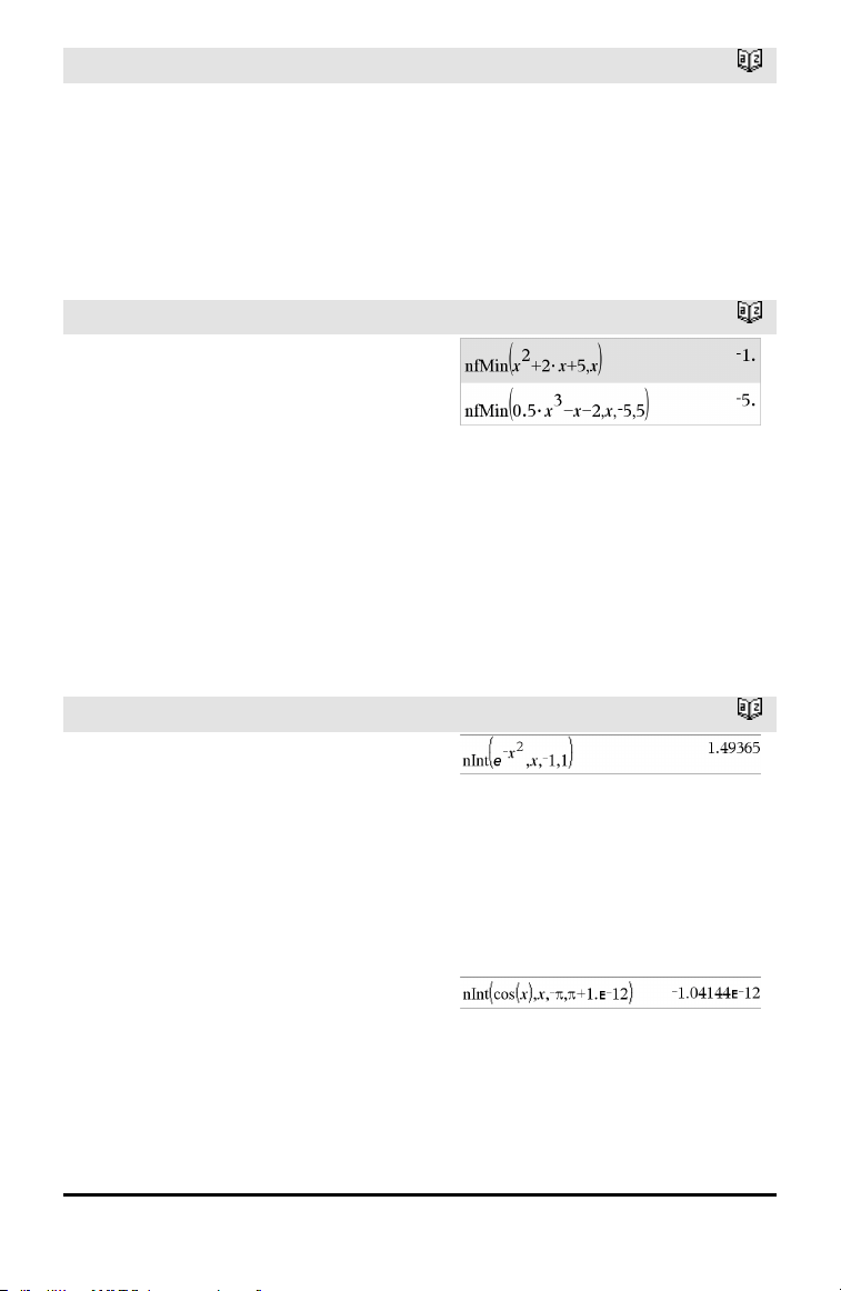
nfMax()
Catalog >
Returns a candidate numerical value of
variable Var where the local maximum of
Expr occurs.
If you supply lowBound and upBound, the
function looks in the closed interval
[lowBound,upBound] for the local
maximum.
nfMin()
Catalog >
nfMin(Expr, Var) ⇒ value
nfMin(Expr, Var, lowBound) ⇒ value
nfMin(Expr, Var, lowBound, upBound) ⇒
value
nfMin(Expr, Var) |
lowBound≤Var≤upBound ⇒ value
Returns a candidate numerical value of
variable Var where the local minimum of
Expr occurs.
If you supply lowBound and upBound, the
function looks in the closed interval
[lowBound,upBound] for the local
minimum.
nInt()
Catalog >
nInt(Expr1, Var, Lower, Upper) ⇒
expression
If the integrand Expr1 contains no variable
other than Var, and if Lower and Upper
are constants, positive ∞, or negative ∞,
then nInt() returns an approximation of ∫
(Expr1, Var, Lower, Upper). This
approximation is a weighted average of
some sample values of the integrand in the
interval Lower<Var<Upper.
The goal is six significant digits. The
adaptive algorithm terminates when it
seems likely that the goal has been
achieved, or when it seems unlikely that
additional samples will yield a worthwhile
improvement.
Alphabetical Listing 101

102 Alphabetical Listing
nInt()
Catalog >
A warning is displayed (“Questionable
accuracy”) when it seems that the goal has
not been achieved.
Nest nInt() to do multiple numeric
integration. Integration limits can depend
on integration variables outside them.
nom()
Catalog >
nom(effectiveRate,CpY) ⇒ value
Financial function that converts the annual
effective interest rate effectiveRate to a
nominal rate, given CpY as the number of
compounding periods per year.
effectiveRate must be a real number, and
CpY must be a real number > 0.
Note: See also eff(), page 44.
nor
/= keys
BooleanExpr1 nor BooleanExpr2 returns
Boolean expression
BooleanList1 nor BooleanList2 returns
Boolean list
BooleanMatrix1 nor BooleanMatrix2
returns Boolean matrix
Returns the negation of a logical or
operation on the two arguments. Returns
true, false, or a simplified form of the
equation.
For lists and matrices, returns comparisons
element by element.
Integer1 nor Integer2 ⇒ integer
Compares two real integers bit-by-bit using
a nor operation. Internally, both integers
are converted to signed, 64-bit binary
numbers. When corresponding bits are
compared, the result is 1 if both bits are 1;
otherwise, the result is 0. The returned
value represents the bit results, and is
displayed according to the Base mode.
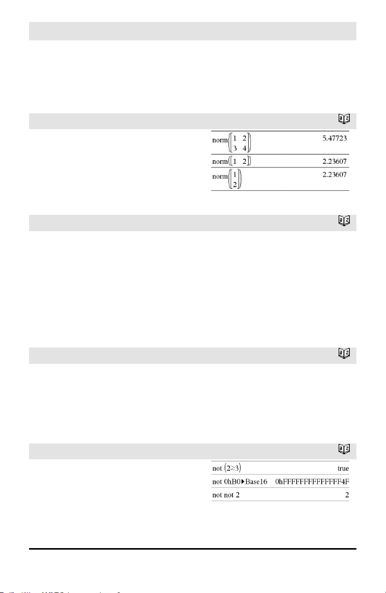
nor
/= keys
You can enter the integers in any number
base. For a binary or hexadecimal entry, you
must use the 0b or 0h prefix, respectively.
Without a prefix, integers are treated as
decimal (base10).
norm()
Catalog >
norm(Matrix) ⇒ expression
norm(Vector) ⇒ expression
Returns the Frobenius norm.
normCdf()
Catalog >
normCdf(lowBound,upBound[,μ[,σ]]) ⇒
number if lowBound and upBound are
numbers, list if lowBound and upBound are
lists
Computes the normal distribution probability
between lowBound and upBound for the
specified μ (default=0) and σ (default=1).
For P(X ≤ upBound), set lowBound = ⁻9E999.
normPdf()
Catalog >
normPdf(XVal[,μ[,σ]]) ⇒ number if XVal is
a number, list if XVal is a list
Computes the probability density function
for the normal distribution at a specified
XVal value for the specified μ and σ.
not
Catalog >
not BooleanExpr ⇒ Boolean expression
Returns true, false, or a simplified form of
the argument.
not Integer1 ⇒ integer
In Hex base mode:
Alphabetical Listing 103
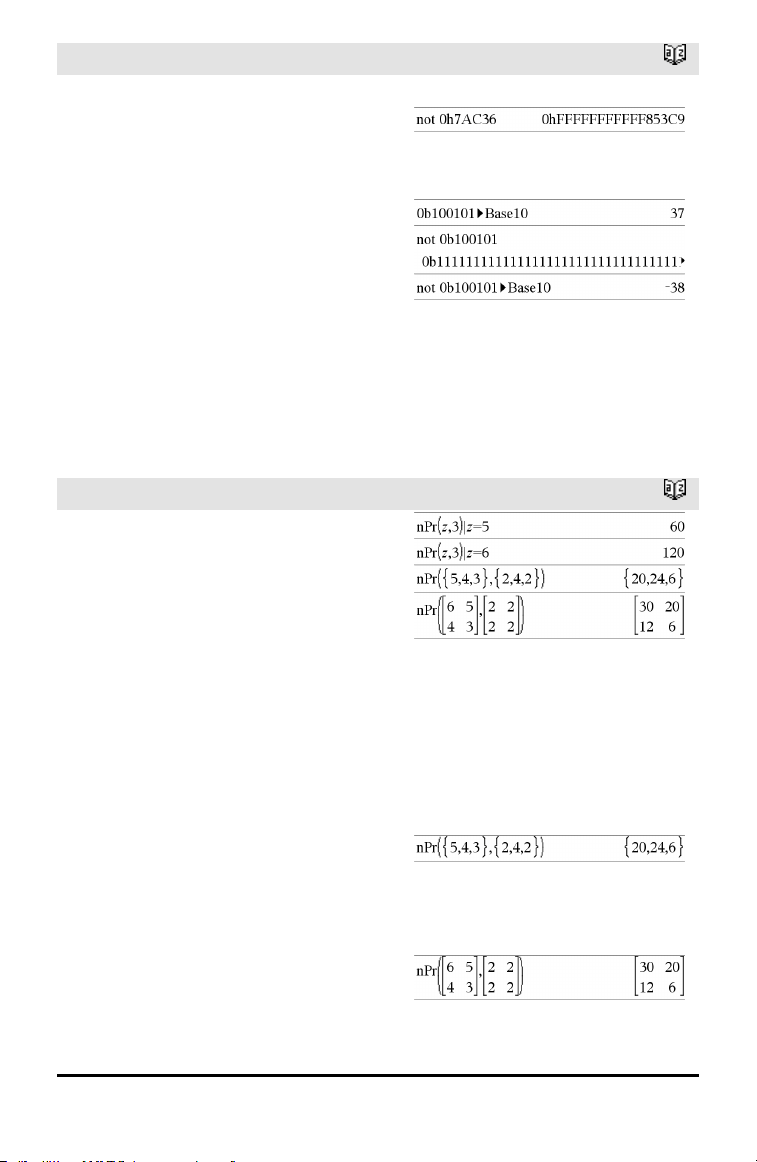
104 Alphabetical Listing
not
Catalog >
Returns the one’s complement of a real
integer. Internally, Integer1 is converted to
a signed, 64-bit binary number. The value of
each bit is flipped (0 becomes 1, and vice
versa) for the one’s complement. Results
are displayed according to the Base mode.
You can enter the integer in any number
base. For a binary or hexadecimal entry, you
must use the 0b or 0h prefix, respectively.
Without a prefix, the integer is treated as
decimal (base10).
If you enter a decimal integer that is too
large for a signed, 64-bit binary form, a
symmetric modulo operation is used to
bring the value into the appropriate range.
For more information, see ►Base2, page
16.
Important: Zero, not the letter O.
In Bin base mode:
To see the entire result, press £ and then
use ¡and¢ to move the cursor.
Note: A binary entry can have up to 64 digits
(not counting the 0b prefix). A hexadecimal
entry can have upto 16 digits.
nPr()
Catalog >
nPr(Value1, Value2) ⇒ expression
For integer Value1 and Value2 with
Value1 ≥ Value2 ≥ 0, nPr() is the number
of permutations of Value1 things taken
Value2 at a time.
nPr(Value, 0) ⇒ 1
nPr(Value, negInteger) ⇒ 1 / ((Value+1)•
(Value+2)...(Value−negInteger))
nPr(Value, posInteger) ⇒ Value•
(Value−1) ... (Value−posInteger+1)
nPr(Value, nonInteger) ⇒ Value! /
(Value−nonInteger)!
nPr(List1, List2) ⇒ list
Returns a list of permutations based on the
corresponding element pairs in the two
lists. The arguments must be the same size
list.
nPr(Matrix1, Matrix2) ⇒ matrix
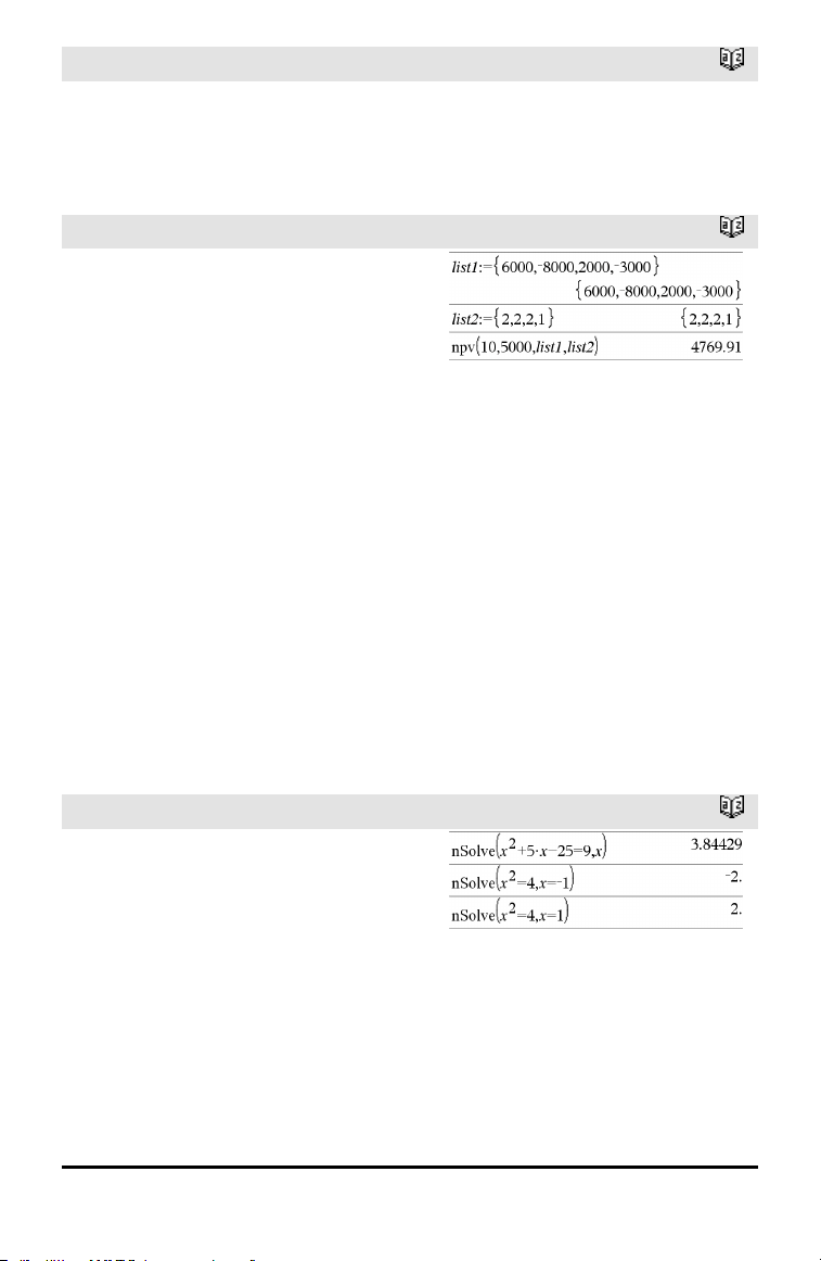
nPr()
Catalog >
Returns a matrix of permutations based on
the corresponding element pairs in the two
matrices. The arguments must be the same
size matrix.
npv()
Catalog >
npv(InterestRate,CFO,CFList[,CFFreq])
Financial function that calculates net
present value; the sum of the present
values for the cash inflows and outflows. A
positive result for npv indicates a profitable
investment.
InterestRate is the rate by which to
discount the cash flows (the cost of money)
over one period.
CF0 is the initial cash flow at time 0; it
must be a real number.
CFList is a list of cash flow amounts after
the initial cash flow CF0.
CFFreq is a list in which each element
specifies the frequency of occurrence for a
grouped (consecutive) cash flow amount,
which is the corresponding element of
CFList. The default is 1; if you enter
values, they must be positive integers <
10,000.
nSolve()
Catalog >
nSolve(Equation,Var[=Guess]) ⇒ number
or error_string
nSolve(Equation,Var[=Guess],lowBound)
⇒ number or error_string
nSolve(Equation,Var
[=Guess],lowBound,upBound) ⇒ number
or error_string
nSolve(Equation,Var[=Guess]) |
lowBound≤Var≤upBound ⇒ number or
error_string
Note: If there are multiple solutions, you can
use a guess to helpfind a particular solution.
Alphabetical Listing 105

106 Alphabetical Listing
nSolve()
Catalog >
Iteratively searches for one approximate
real numeric solution to Equation for its
one variable. Specify the variable as:
variable
– or –
variable = real number
For example, x is valid and so is x=3.
nSolve() attempts to determine either one
point where the residual is zero or two
relatively close points where the residual
has opposite signs and the magnitude of
the residual is not excessive. If it cannot
achieve this using a modest number of
sample points, it returns the string “no
solution found.”
O
OneVar
Catalog >
OneVar [1,]X[,[Freq][,Category,Include]]
OneVar [n,]X1,X2[X3[,…[,X20]]]
Calculates 1-variable statistics on up to 20
lists. A summary of results is stored in the
stat.results variable. (See page 145.)
All the lists must have equal dimension
except for Include.
Freq is an optional list of frequency values.
Each element in Freq specifies the
frequency of occurrence for each
corresponding X and Y data point. The
default value is 1. All elements must be
integers ≥ 0.
Category is a list of numeric category codes
for the corresponding X values.
Include is a list of one or more of the
category codes. Only those data items
whose category code is included in this list
are included in the calculation.
OneVar
Catalog >
An empty (void) element in any of the lists
X, Freq, or Category results in a void for
the corresponding element of all those lists.
An empty element in any of the lists X1
through X20 results in a void for the
corresponding element of all those lists. For
more information on empty elements, see
page 196.
Output variable Description
stat.v Mean of x values
stat.Σx
Sum of x values
stat.Σx
2
Sum of x
2
values
stat.sx Sample standard deviation of x
stat.σx
Population standard deviation of x
stat.n Number of data points
stat.MinX Minimum of x values
stat.Q
1
X 1st Quartile of x
stat.MedianX Median of x
stat.Q
3
X 3rd Quartile of x
stat.MaxX Maximum of x values
stat.SSX Sum of squares of deviations from the mean of x
or
Catalog >
BooleanExpr1 or BooleanExpr2 returns
Boolean expression
BooleanList1 or BooleanList2 returns
Boolean list
BooleanMatrix1 or BooleanMatrix2
returns Boolean matrix
Returns true or false or a simplified form of
the original entry.
Returns true if either or both expressions
simplify to true. Returns false only if both
expressions evaluate to false.
Note: See xor.
Alphabetical Listing 107
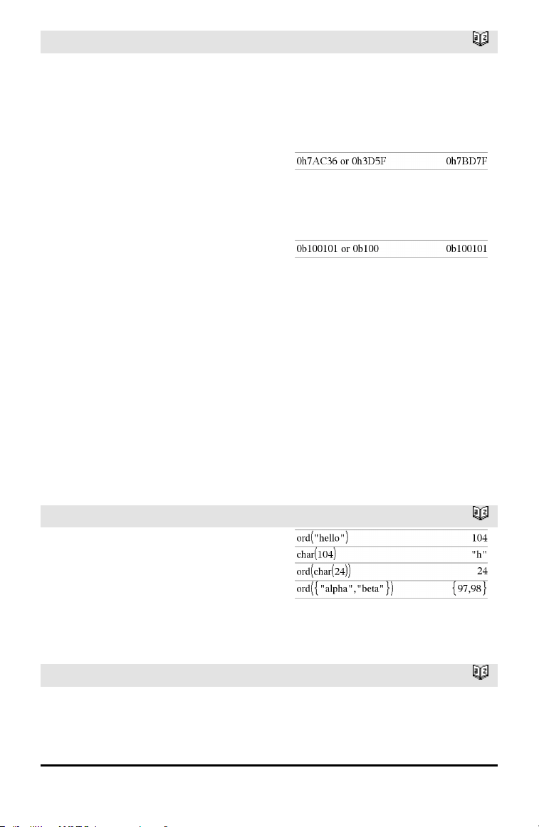
108 Alphabetical Listing
or
Catalog >
Note for entering the example: For
instructions on entering multi-line program
and function definitions, refer to the
Calculator section of your product
guidebook.
Integer1 or Integer2 ⇒ integer
Compares two real integers bit-by-bit using
an or operation. Internally, both integers
are converted to signed, 64-bit binary
numbers. When corresponding bits are
compared, the result is 1 if either bit is 1;
the result is 0 only if both bits are 0. The
returned value represents the bit results,
and is displayed according to the Base
mode.
You can enter the integers in any number
base. For a binary or hexadecimal entry, you
must use the 0b or 0h prefix, respectively.
Without a prefix, integers are treated as
decimal (base10).
If you enter a decimal integer that is too
large for a signed, 64-bit binary form, a
symmetric modulo operation is used to
bring the value into the appropriate range.
For more information, see ►Base2, page
16.
Note: See xor.
In Hex base mode:
Important: Zero, not the letter O.
In Bin base mode:
Note: A binary entry can have up to 64 digits
(not counting the 0b prefix). A hexadecimal
entry can have upto 16 digits.
ord()
Catalog >
ord(String) ⇒ integer
ord(List1) ⇒ list
Returns the numeric code of the first
character in character string String, or a list
of the first characters of each list element.
P
P►Rx()
Catalog >
P►Rx(rExpr, θExpr) ⇒ expression
P►Rx(rList, θList) ⇒ list
P►Rx(rMatrix, θMatrix) ⇒ matrix
In Radian angle mode:
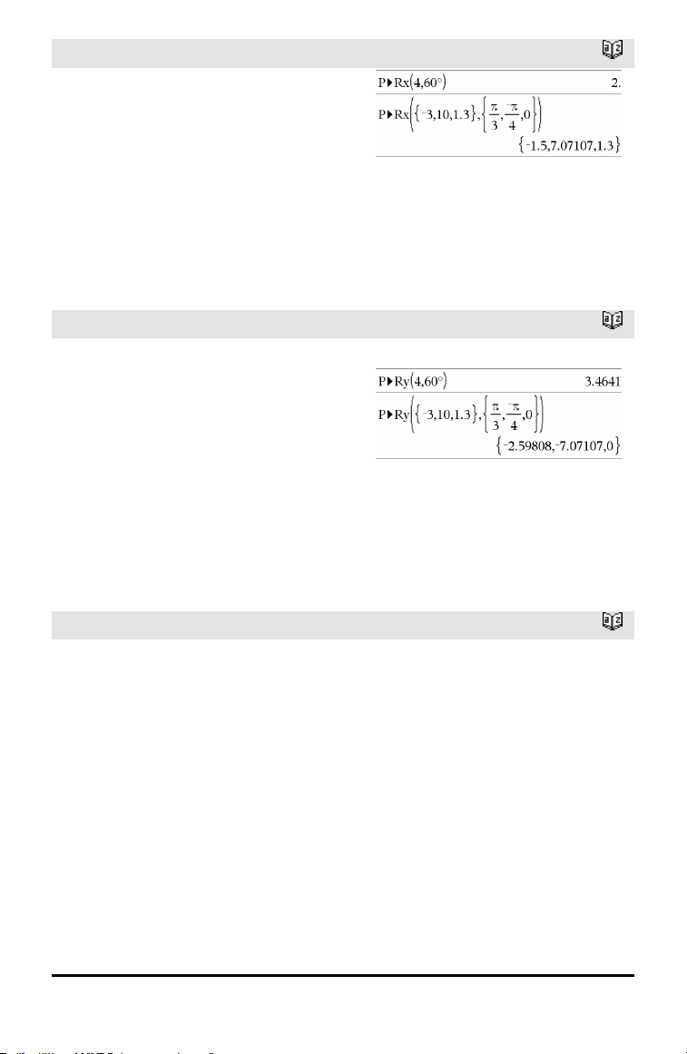
P►Rx()
Catalog >
Returns the equivalent x-coordinate of the
(r,θ) pair.
Note: The θ argument is interpreted as
either a degree, gradian or radian angle,
according to the current angle mode. If the
argument is an expression, you can use°,
G
,
or
r
to override the angle mode setting
temporarily.
Note: You can insert this function from the
computer keyboard by typing P@>Rx(...).
P►Ry()
Catalog >
P►Ry(rValue, θValue) ⇒ value
P►Ry(rList, θList) ⇒ list
P►Ry(rMatrix, θMatrix) ⇒ matrix
Returns the equivalent y-coordinate of the
(r,θ) pair.
Note: The θ argument is interpreted as
either a degree, radian or gradian angle,
according to the current angle mode.°
r
Note: You can insert this function from the
computer keyboard by typing P@>Ry(...).
In Radian angle mode:
PassErr
Catalog >
PassErr
Passes an error to the next level.
If system variable errCode is zero, PassErr
does not do anything.
The Else clause of the Try...Else...EndTry
block should use ClrErr or PassErr. If the
error is to be processed or ignored, use
ClrErr. If what to do with the error is not
known, use PassErr to send it to the next
error handler. If there are no more pending
Try...Else...EndTry error handlers, the error
dialog box will be displayed as normal.
Note: See also ClrErr, page 22, and Try, page
157.
For an example of PassErr, See Example 2
under the Try command, page 157.
Alphabetical Listing 109

110 Alphabetical Listing
PassErr
Catalog >
Note for entering the example: For
instructions on entering multi-line program
and function definitions, refer to the
Calculator section of your product guidebook.
piecewise()
Catalog >
piecewise(Expr1[, Cond1[, Expr2 [, Cond2
[, … ]]]])
Returns definitions for a piecewise function
in the form of a list. You can also create
piecewise definitions by using a template.
Note: See also Piecewise template, page 2.
poissCdf()
Catalog >
poissCdf(λ,lowBound,upBound) ⇒ number
if lowBound and upBound are numbers, list
if lowBound and upBound are lists
poissCdf(λ,upBound)for P(0≤X≤upBound) ⇒
number if upBound is a number, list if
upBound is a list
Computes a cumulative probability for the
discrete Poisson distribution with specified
mean λ.
For P(X ≤ upBound), set lowBound=0
poissPdf()
Catalog >
poissPdf(λ,XVal) ⇒ number if XVal is a
number, list if XVal is a list
Computes a probability for the discrete
Poisson distribution with the specified mean
λ.
►Polar
Catalog >
Vector ►Polar
Note: You can insert this operator from the
computer keyboard by typing @>Polar.
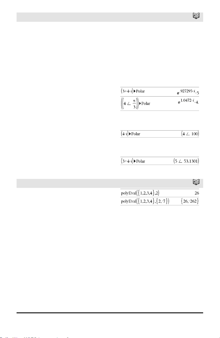
►Polar
Catalog >
Displays vector in polar form [r∠θ]. The
vector must be of dimension 2 and can be a
row or a column.
Note: ►Polar is a display-format
instruction, not a conversion function. You
can use it only at the end of an entry line,
and it does not update ans.
Note: See also ►Rect, page 122.
complexValue ►Polar
Displays complexVector in polar form.
• Degree angle mode returns (r∠θ).
• Radian angle mode returns re
iθ
.
complexValue can have any complex form.
However, an re
iθ
entry causes an error in
Degree angle mode.
Note: You must use the parentheses for an
(r∠θ) polar entry.
In Radian angle mode:
In Gradian angle mode:
In Degree angle mode:
polyEval()
Catalog >
polyEval(List1, Expr1) ⇒ expression
polyEval(List1, List2) ⇒ expression
Interprets the first argument as the
coefficient of a descending-degree
polynomial, and returns the polynomial
evaluated for the value of the second
argument.
Alphabetical Listing 111

112 Alphabetical Listing
polyRoots()
Catalog >
polyRoots(Poly,Var) ⇒ list
polyRoots(ListOfCoeffs) ⇒ list
The first syntax, polyRoots(Poly,Var),
returns a list of real roots of polynomial
Poly with respect to variable Var. If no real
roots exist, returns an empty list: {}.
Poly must be a polynomial in expanded
form in one variable. Do not use
unexpanded forms such as y
2
•y+1 or
x•x+2•x+1
The second syntax, polyRoots
(ListOfCoeffs), returns a list of real roots
for the coefficients in ListOfCoeffs.
Note: See also cPolyRoots(), page 30.
PowerReg
Catalog >
PowerReg X,Y[, Freq][, Category, Include]]
Computes the power regressiony = (a•(x)
b
)
on lists X and Y with frequency Freq. A
summary of results is stored in the
stat.results variable. (See page 145.)
All the lists must have equal dimension
except for Include.
X and Y are lists of independent and
dependent variables.
Freq is an optional list of frequency values.
Each element in Freq specifies the
frequency of occurrence for each
corresponding X and Y data point. The
default value is 1. All elements must be
integers ≥ 0.
Category is a list of numeric or string
category codes for the corresponding X and
Y data.
Include is a list of one or more of the
category codes. Only those data items
whose category code is included in this list
are included in the calculation.

PowerReg
Catalog >
For information on the effect of empty
elements in a list, see “Empty (Void)
Elements,” page 196.
Output
variable
Description
stat.RegEqn
Regression equation: a•(x)
b
stat.a, stat.b Regression coefficients
stat.r
2
Coefficientof linear determination for transformeddata
stat.r Correlation coefficient for transformed data (ln(x), ln(y))
stat.Resid Residuals associated with the power model
stat.ResidTrans Residuals associated with linear fitof transformed data
stat.XReg
Listof data points in the modifiedX List actually used in the regression based on
restrictions of Freq, Category List, and Include Categories
stat.YReg
Listof data points in the modifiedY List actually used inthe regression basedon
restrictions of Freq, Category List, and Include Categories
stat.FreqReg
Listof frequencies corresponding to stat.XReg and stat.YReg
Prgm
Catalog >
Prgm
Block
EndPrgm
Template for creating a user-defined
program. Must be used with the Define,
Define LibPub, or Define LibPriv command.
Block can be a single statement, a series
of statements separated with the “:”
character, or a series of statements on
separate lines.
Note for entering the example: For
instructions on entering multi-line program
and function definitions, refer to the
Calculator section of your product
guidebook.
Calculate GCD and display intermediate
results.
Alphabetical Listing 113
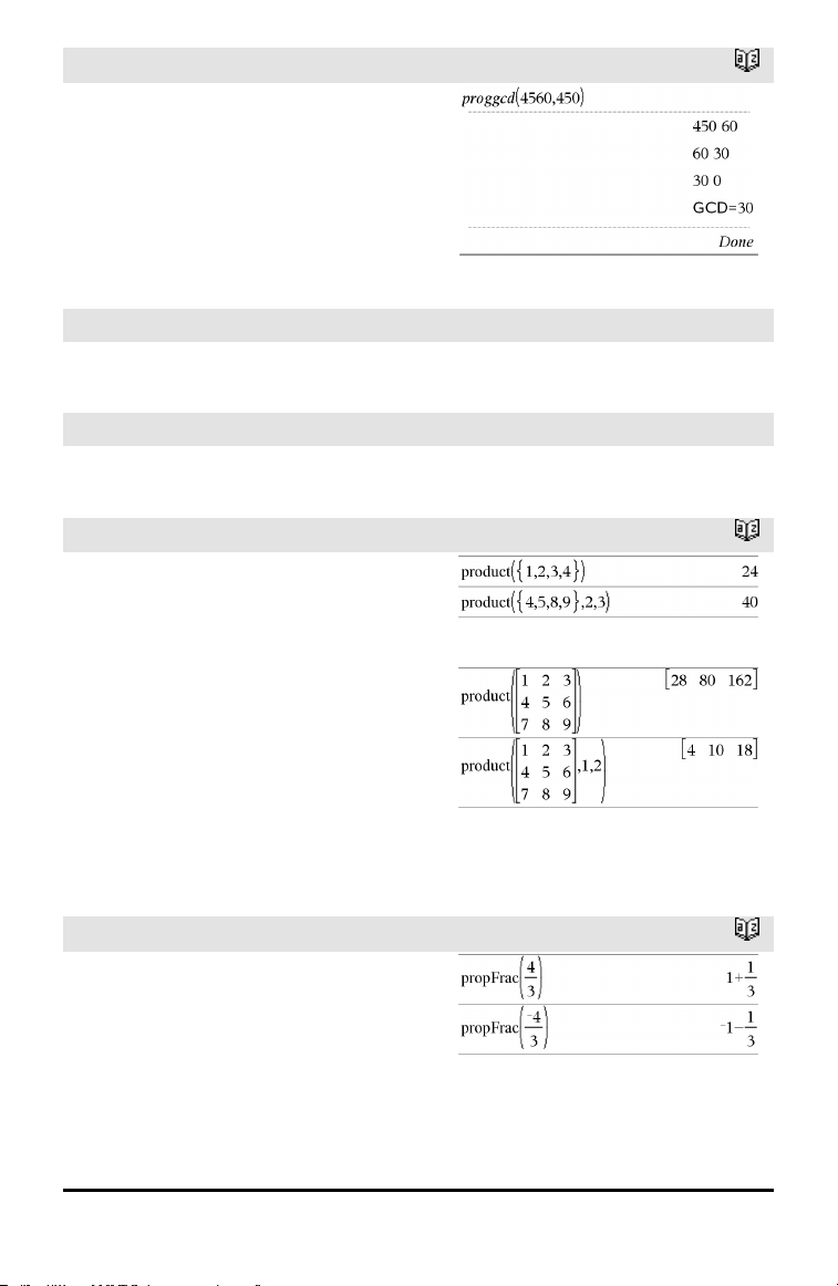
114 Alphabetical Listing
Prgm
Catalog >
prodSeq()
See Π (), page 185.
Product (PI)
See Π (), page 185.
product()
Catalog >
product(List[, Start[, End]]) ⇒ expression
Returns the product of the elements
contained in List. Start and End are
optional. They specify a range of elements.
product(Matrix1[, Start[, End]]) ⇒ matrix
Returns a row vector containing the
products of the elements in the columns of
Matrix1. Start and end are optional. They
specify a range of rows.
Empty (void) elements are ignored. For
more information on empty elements, see
page 196.
propFrac()
Catalog >
propFrac(Value1[, Var]) ⇒ value
propFrac(rational_number) returns
rational_number as the sum of an integer
and a fraction having the same sign and a
greater denominator magnitude than
numerator magnitude.
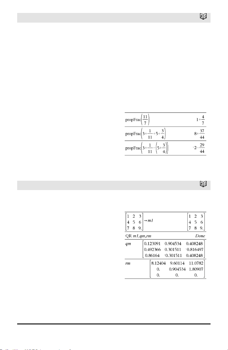
propFrac()
Catalog >
propFrac(rational_expression,Var) returns
the sum of proper ratios and a polynomial
with respect to Var. The degree of Var in
the denominator exceeds the degree of Var
in the numerator in each proper ratio.
Similar powers of Var are collected. The
terms and their factors are sorted with Var
as the main variable.
If Var is omitted, a proper fraction
expansion is done with respect to the most
main variable. The coefficients of the
polynomial part are then made proper with
respect to their most main variable first
and so on.
You can use the propFrac() function to
represent mixed fractions and demonstrate
addition and subtraction of mixed fractions.
Q
QR
Catalog >
QR Matrix, qMatrix, rMatrix[, Tol]
Calculates the Householder QR factorization
of a real or complex matrix. The resulting Q
and R matrices are stored to the specified
Matrix. The Q matrix is unitary. The R
matrix is upper triangular.
Optionally, any matrix element is treated as
zero if its absolute value is less than Tol.
This tolerance is used only if the matrix has
floating-point entries and does not contain
any symbolic variables that have not been
assigned a value. Otherwise, Tol is ignored.
• If you use /· or set the Auto or
Approximate mode to Approximate,
computations are done using floating-
point arithmetic.
• If Tol is omitted or not used, the default
The floating-point number (9.) inm1 causes
results to be calculated in floating-point
form.
Alphabetical Listing 115

116 Alphabetical Listing
QR
Catalog >
tolerance is calculated as:
5E−14 •max(dim(Matrix)) •rowNorm
(Matrix)
The QR factorization is computed
numerically using Householder
transformations. The symbolic solution is
computed using Gram-Schmidt. The
columns in qMatName are the orthonormal
basis vectors that span the space defined by
matrix.
QuadReg
Catalog >
QuadReg X,Y[, Freq][, Category, Include]]
Computes the quadratic polynomial
regression y=a•x
2
+b•x+c on lists X and Y
with frequency Freq. A summary of results
is stored in the stat.results variable. (See
page 145.)
All the lists must have equal dimension
except for Include.
X and Y are lists of independent and
dependent variables.
Freq is an optional list of frequency values.
Each element in Freq specifies the
frequency of occurrence for each
corresponding X and Y data point. The
default value is 1. All elements must be
integers ≥ 0.
Category is a list of numeric or string
category codes for the corresponding X and
Y data.
Include is a list of one or more of the
category codes. Only those data items
whose category code is included in this list
are included in the calculation.
For information on the effect of empty
elements in a list, see “Empty (Void)
Elements,” page 196.
Output
variable
Description

stat.RegEqn
Regression equation: a•x
2
+b•x+c
stat.a,
stat.b, stat.c
Regression coefficients
stat.R
2
Coefficientof determination
stat.Resid Residuals from the regression
stat.XReg
Listof data points in the modifiedX List actually used in the regression based on
restrictions of Freq, Category List, and Include Categories
stat.YReg
Listof data points in the modifiedY List actually used inthe regression basedon
restrictions of Freq, Category List, and Include Categories
stat.FreqReg
Listof frequencies corresponding to stat.XReg and stat.YReg
QuartReg
Catalog >
QuartReg X,Y[, Freq][, Category, Include]]
Computes the quartic polynomial regression
y = a•x
4
+b•x
3
+c• x
2
+d•x+e on lists X and Y
with frequency Freq. A summary of results
is stored in the stat.results variable. (See
page 145.)
All the lists must have equal dimension
except for Include.
X and Y are lists of independent and
dependent variables.
Freq is an optional list of frequency values.
Each element in Freq specifies the
frequency of occurrence for each
corresponding X and Y data point. The
default value is 1. All elements must be
integers ≥ 0.
Category is a list of numeric or string
category codes for the corresponding X and
Y data.
Include is a list of one or more of the
category codes. Only those data items
whose category code is included in this list
are included in the calculation.
For information on the effect of empty
elements in a list, see “Empty (Void)
Elements,” page 196.
Alphabetical Listing 117
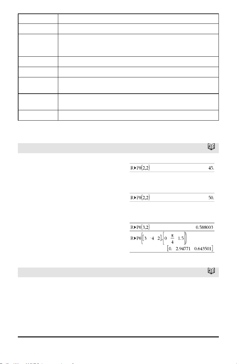
118 Alphabetical Listing
Output variable Description
stat.RegEqn
Regression equation: a•x
4
+b•x
3
+c• x
2
+d•x+e
stat.a, stat.b,
stat.c, stat.d,
stat.e
Regression coefficients
stat.R
2
Coefficientof determination
stat.Resid Residuals from the regression
stat.XReg
Listof data points in the modifiedX List actually used in the regression based on
restrictions of Freq, Category List, and Include Categories
stat.YReg
Listof data points in the modifiedY List actually used inthe regression basedon
restrictions of Freq, Category List, and Include Categories
stat.FreqReg
Listof frequencies corresponding to stat.XReg and stat.YReg
R
R►Pθ()
Catalog >
R►Pθ (xValue, yValue) ⇒ value
R►Pθ (xList, yList) ⇒ list
R►Pθ (xMatrix, yMatrix) ⇒ matrix
Returns the equivalent θ-coordinate of the
(x,y) pair arguments.
Note: The result is returned as a degree,
gradian or radian angle, according to the
current angle mode setting.
Note: You can insert this function from the
computer keyboard by typing R@>Ptheta
(...).
In Degree angle mode:
In Gradian angle mode:
In Radian angle mode:
R►Pr()
Catalog >
R►Pr (xValue, yValue) ⇒ value
R►Pr (xList, yList) ⇒ list
R►Pr (xMatrix, yMatrix) ⇒ matrix
Returns the equivalent r-coordinate of the
(x,y) pair arguments.
In Radian angle mode:
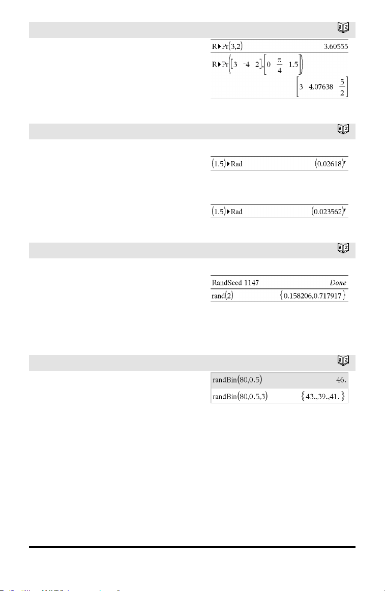
R►Pr()
Catalog >
Note: You can insert this function from the
computer keyboard by typing R@>Pr(...).
►Rad
Catalog >
Value1►Rad
⇒
value
Converts the argument to radian angle
measure.
Note: You can insert this operator from the
computer keyboard by typing @>Rad.
In Degree angle mode:
In Gradian angle mode:
rand()
Catalog >
rand() ⇒ expression
rand(#Trials) ⇒ list
rand() returns a random value between 0
and 1.
rand(#Trials) returns a list containing
#Trials random values between 0 and 1.
Set the random-number seed.
randBin()
Catalog >
randBin(n, p) ⇒ expression
randBin(n, p, #Trials) ⇒ list
randBin(n, p) returns a random real number
from a specified Binomial distribution.
randBin(n, p, #Trials) returns a list
containing #Trials random real numbers
from a specified Binomial distribution.
Alphabetical Listing 119
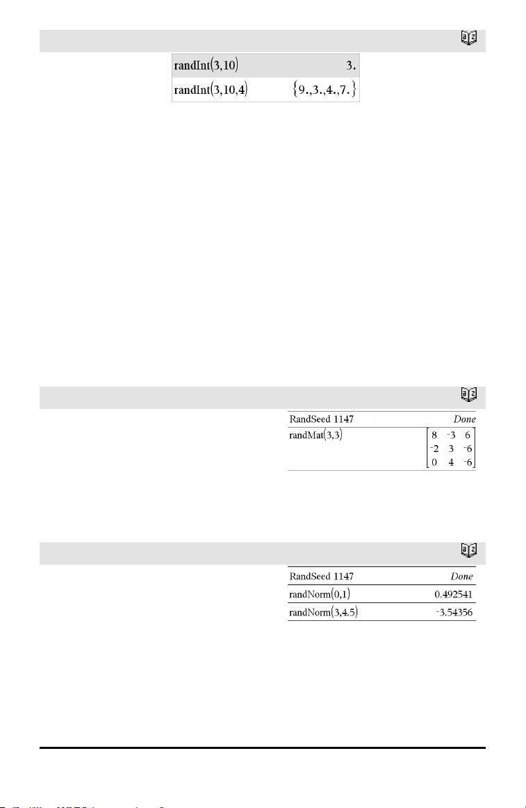
120 Alphabetical Listing
randInt()
Catalog >
randInt
(lowBound,upBound)
⇒ expression
randInt
(lowBound,upBound
,#Trials) ⇒ list
randInt
(lowBound,upBound)
returns a random
integer within the
range specified by
lowBound and
upBound integer
bounds.
randInt
(lowBound,upBound
,#Trials) returns a
list containing
#Trials random
integers within the
specified range.
randMat()
Catalog >
randMat(numRows, numColumns) ⇒
matrix
Returns a matrix of integers between -9
and 9 of the specified dimension.
Both arguments must simplify to integers.
Note: The values in this matrix will change
each time you press ·.
randNorm()
Catalog >
randNorm(μ, σ) ⇒ expression
randNorm(μ, σ, #Trials) ⇒ list
randNorm(μ, σ) returns a decimal number
from the specified normal distribution. It
could be any real number but will be heavily
concentrated in the interval [μ−3•σ, μ+3•σ].
randNorm(μ, σ, #Trials) returns a list
containing #Trials decimal numbers from
the specified normal distribution.
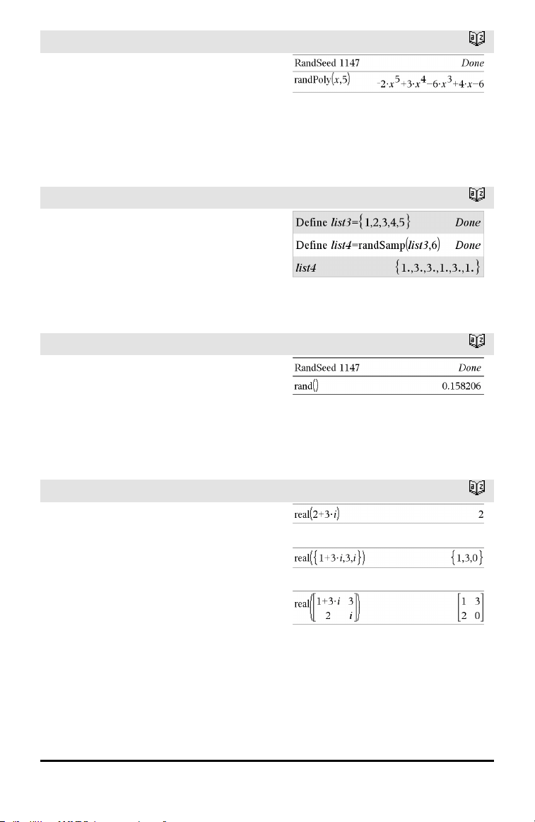
randPoly()
Catalog >
randPoly(Var, Order) ⇒ expression
Returns a polynomial in Var of the
specified Order. The coefficients are
random integers in the range −9 through 9.
The leading coefficient will not be zero.
Order must be 0–99.
randSamp()
Catalog >
randSamp(List,#Trials[,noRepl]) ⇒ list
Returns a list containing a random sample
of #Trials trials from List with an option
for sample replacement (noRepl=0), or no
sample replacement (noRepl=1). The
default is with sample replacement.
RandSeed
Catalog >
RandSeed Number
If Number = 0, sets the seeds to the factory
defaults for the random-number generator.
If Number ≠0, it is used to generate two
seeds, which are stored in system variables
seed1 andseed2.
real()
Catalog >
real(Value1) ⇒ value
Returns the real part of the argument.
real(List1) ⇒ list
Returns the real parts of all elements.
real(Matrix1) ⇒ matrix
Returns the real parts of all elements.
Alphabetical Listing 121
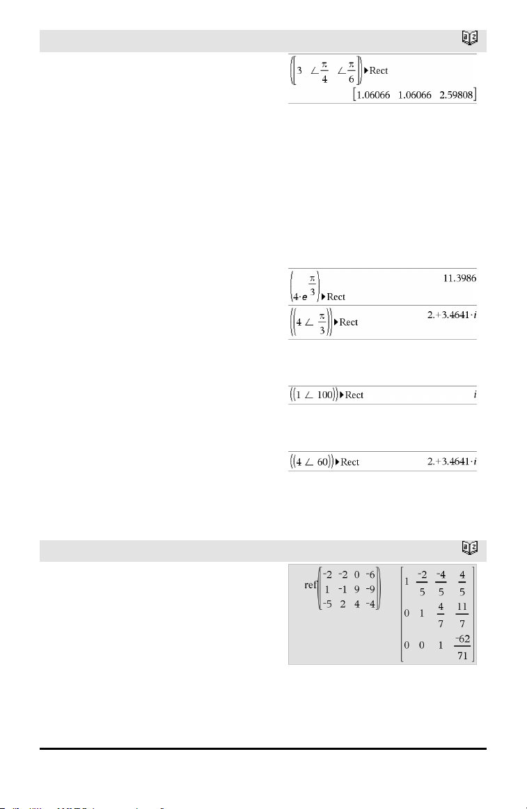
122 Alphabetical Listing
►Rect
Catalog >
Vector ►Rect
Note: You can insert this operator from the
computer keyboard by typing @>Rect.
Displays Vector in rectangular form [x, y,
z]. The vector must be of dimension 2 or 3
and can be a row or a column.
Note: ►Rect is a display-format instruction,
not a conversion function. You can use it
only at the end of an entry line, and it does
not update ans.
Note: See also ►Polar, page 110.
complexValue ►Rect
Displays complexValue in rectangular form
a+bi. The complexValue can have any
complex form. However, an re
iθ
entry
causes an error in Degree angle mode.
Note: You must use parentheses for an
(r∠θ) polar entry.
In Radian angle mode:
In Gradian angle mode:
In Degree angle mode:
Note: To type ∠, select itfrom the symbol
listin the Catalog.
ref()
Catalog >
ref(Matrix1[, Tol]) ⇒ matrix
Returns the row echelon form of Matrix1.
Optionally, any matrix element is treated as
zero if its absolute value is less than Tol.
This tolerance is used only if the matrix has
floating-point entries and does not contain
any symbolic variables that have not been
assigned a value. Otherwise, Tol is ignored.
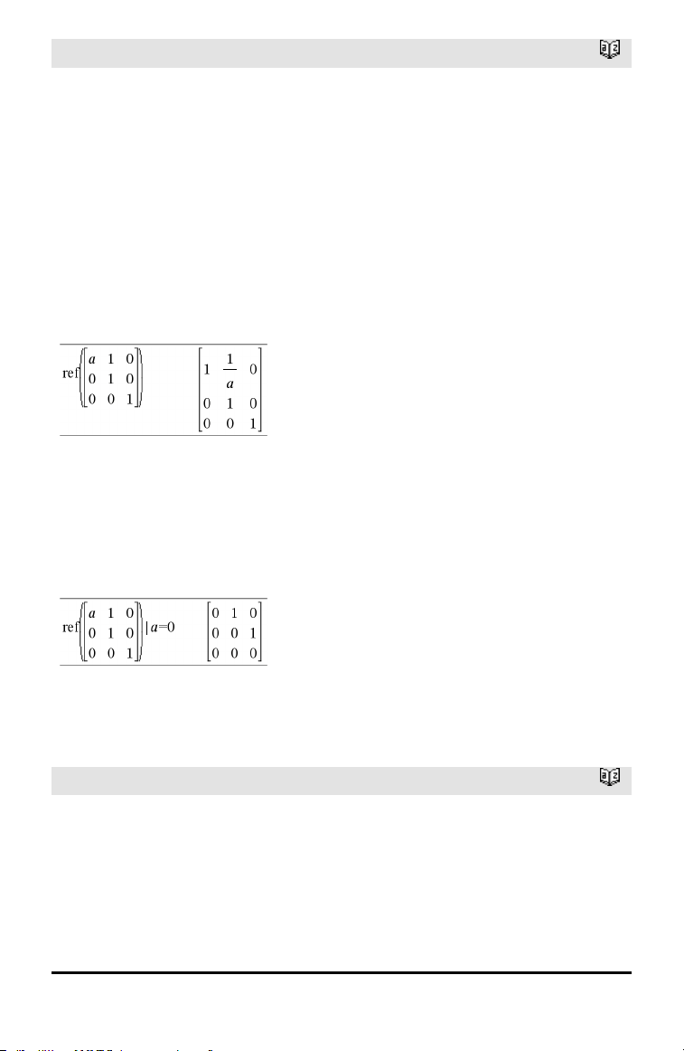
ref()
Catalog >
• If you use /· or set the Auto or
Approximate mode to Approximate,
computations are done using floating-
point arithmetic.
• If Tol is omitted or not used, the default
tolerance is calculated as:
5E−14 •max(dim(Matrix1)) •rowNorm
(Matrix1)
Avoid undefined elements in Matrix1. They
can lead to unexpected results.
For example, if a is undefined in the
following expression, a warning message
appears and the result is shown as:
The warning appears because the
generalized element 1/a would not be valid
for a=0.
You can avoid this by storing a value to a
beforehand or by using the constraint (“|”)
operator to substitute a value, as shown in
the following example.
Note: See also rref(), page 132.
RefreshProbeVars
Catalog >
RefreshProbeVars
Allows you to access sensor data from all
connected sensor probes in your TI-Basic
program.
Example
Define temp()=
Prgm
© Check if system is ready
RefreshProbeVars status
Alphabetical Listing 123
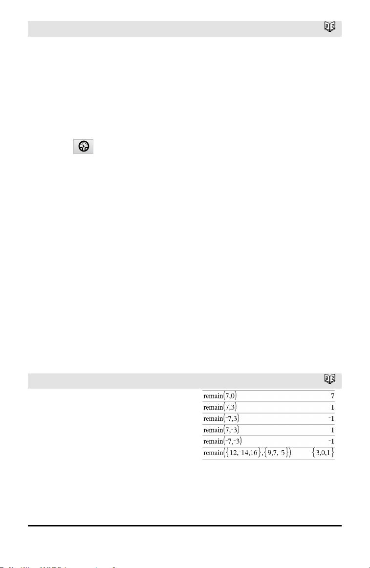
124 Alphabetical Listing
RefreshProbeVars
Catalog >
StatusVar
Value
Status
statusVar
=0
Normal (continue with the
program)
statusVar
=1
The Vernier DataQuest™
application is in data collection
mode.
Note: The Vernier DataQuest™
application must be in meter
mode for this command to work.
statusVar
=2
The Vernier DataQuest™
application is not launched.
statusVar
=3
The Vernier DataQuest™
application is launched, but you
have not connected any probes.
If status=0 Then
Disp "ready"
For n,1,50
RefreshProbeVars status
temperature:=meter.temperature
Disp "Temperature:
",temperature
If temperature>30 Then
Disp "Too hot"
EndIf
© Wait for 1 second between
samples
Wait 1
EndFor
Else
Disp "Not ready. Try again
later"
EndIf
EndPrgm
Note: This can also be used with TI-
Innovator™ Hub.
remain()
Catalog >
remain(Value1, Value2) ⇒ value
remain(List1, List2) ⇒ list
remain(Matrix1, Matrix2) ⇒ matrix
Returns the remainder of the first
argument with respect to the second
argument as defined by the identities:
remain(x,0)x
remain(x,y)x−y•iPart(x/y)
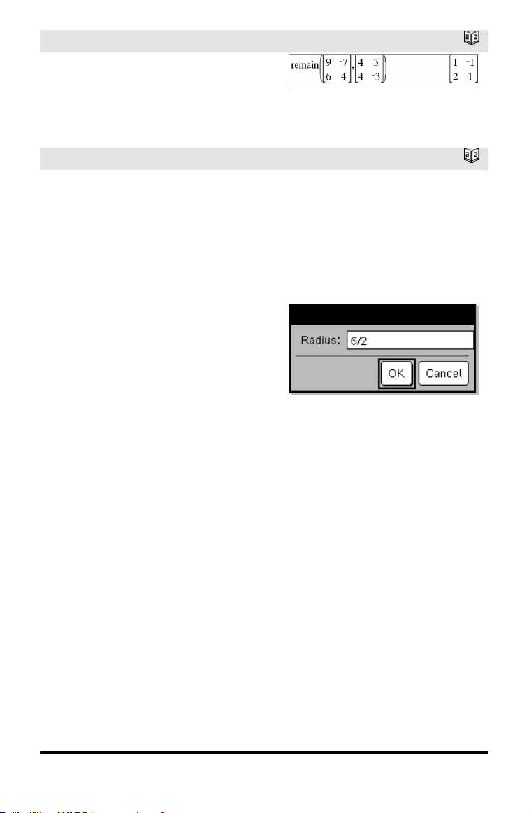
remain()
Catalog >
As a consequence, note that remain(−x,y) −
remain(x,y). The result is either zero or it
has the same sign as the first argument.
Note: See also mod(), page 94.
Request
Catalog >
Request promptString, var[,DispFlag
[,statusVar]]
Request promptString, func(arg1, ...argn)
[,DispFlag [,statusVar]]
Programming command: Pauses the
program and displays a dialog box
containing the message promptString and
an input box for the user’s response.
When the user types a response and clicks
OK, the contents of the input box are
assigned to variable var.
If the user clicks Cancel, the program
proceeds without accepting any input. The
program uses the previous value of var if
var was already defined.
The optional DispFlag argument can be
any expression.
• If DispFlag is omitted or evaluates to 1,
the prompt message and user’s response
are displayed in the Calculator history.
• If DispFlag evaluates to 0, the prompt
and response are not displayed in the
history.
Define a program:
Define request_demo()=Prgm
Request “Radius: ”,r
Disp “Area = “,pi*r
2
EndPrgm
Run the program andtype a response:
request_demo()
Resultafter selecting OK:
Radius: 6/2
Area= 28.2743
The optional statusVar argument gives the
program a way to determine how the user
dismissed the dialog box. Note that
statusVar requires the DispFlag argument.
• If the user clicked OK or pressed Enter or
Ctrl+Enter, variable statusVar is set to a
value of 1.
• Otherwise, variable statusVar is set to a
value of 0.
Define a program:
Define polynomial()=Prgm
Request "Enter a polynomial in
x:",p(x)
Disp "Real roots are:",polyRoots
(p(x),x)
EndPrgm
Run the program andtype a response:
polynomial()
Alphabetical Listing 125

126 Alphabetical Listing
Request
Catalog >
The func() argument allows a program to
store the user’s response as a function
definition. This syntax operates as if the
user executed the command:
Define func(arg1, ...argn) = user’s
response
The program can then use the defined
function func(). The promptString should
guide the user to enter an appropriate
user’sresponse that completes the
function definition.
Note: You can use the Request command
within a user-defined program but not
within a function.
To stop a program that contains a Request
command inside an infinite loop:
• Handheld: Hold down the c key and
press · repeatedly.
• Windows®: Hold down the F12 key and
press Enter repeatedly.
• Macintosh®: Hold down the F5 key and
press Enter repeatedly.
• iPad®: The app displays a prompt. You
can continue waiting or cancel.
Note: See also RequestStr, page 126.
Resultafter entering x^3+3x+1 and selecting
OK:
Real roots are: {-0.322185}
RequestStr
Catalog >
RequestStr promptString, var[, DispFlag]
Programming command: Operates
identically to the first syntax of the Request
command, except that the user’s response
is always interpreted as a string. By
contrast, the Request command interprets
the response as an expression unless the
user encloses it in quotation marks (““).
Note: You can use the RequestStr command
within a user-defined program but not
within a function.
Define a program:
Define requestStr_demo()=Prgm
RequestStr “Your name:”,name,0
Disp “Response has “,dim(name),”
characters.”
EndPrgm
Run the program andtype a response:
requestStr_demo()
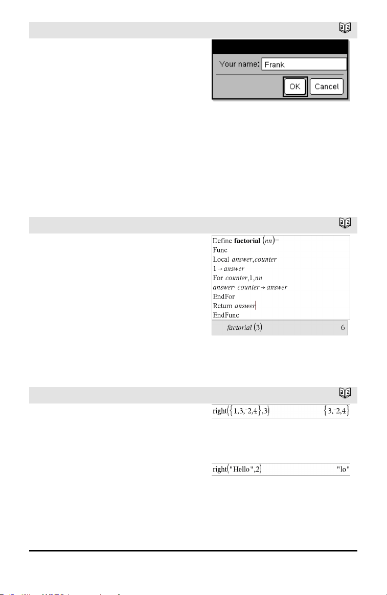
RequestStr
Catalog >
To stop a program that contains a
RequestStr command inside an infinite loop:
• Handheld: Hold down the c key and
press · repeatedly.
• Windows®: Hold down the F12 key and
press Enter repeatedly.
• Macintosh®: Hold down the F5 key and
press Enter repeatedly.
• iPad®: The app displays a prompt. You
can continue waiting or cancel.
Note: See also Request, page 125.
Resultafter selecting OK (Note that the
DispFlag argument of 0 omits the prompt
and response from the history):
requestStr_demo()
Response has 5 characters.
Return
Catalog >
Return [Expr]
Returns Expr as the result of the function.
Use within a Func...EndFunc block.
Note: Use Return without an argument
within a Prgm...EndPrgm block to exit a
program.
Note for entering the example: For
instructions on entering multi-line program
and function definitions, refer to the
Calculator section of your product
guidebook.
right()
Catalog >
right(List1[, Num]) ⇒ list
Returns the rightmost Num elements
contained in List1.
If you omit Num, returns all of List1.
right(sourceString[, Num]) ⇒ string
Returns the rightmost Num characters
contained in character string sourceString.
If you omit Num, returns all of
sourceString.
Alphabetical Listing 127
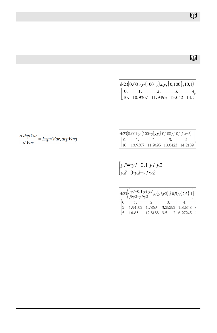
128 Alphabetical Listing
right()
Catalog >
right(Comparison) ⇒ expression
Returns the right side of an equation or
inequality.
rk23 ()
Catalog >
rk23(Expr, Var, depVar, {Var0, VarMax},
depVar0, VarStep [, diftol]) ⇒ matrix
rk23(SystemOfExpr, Var, ListOfDepVars,
{Var0, VarMax}, ListOfDepVars0,
VarStep[, diftol]) ⇒ matrix
rk23(ListOfExpr, Var, ListOfDepVars,
{Var0, VarMax}, ListOfDepVars0,
VarStep[, diftol]) ⇒ matrix
Uses the Runge-Kutta method to solve the
system
with depVar(Var0)=depVar0 on the
interval [Var0,VarMax]. Returns a matrix
whose first row defines the Var output
values as defined by VarStep. The second
row defines the value of the first solution
component at the corresponding Var
values, and so on.
Expr is the right hand side that defines the
ordinary differential equation (ODE).
SystemOfExpr is a system of right-hand
sides that define the system of ODEs
(corresponds to order of dependent
variables in ListOfDepVars).
ListOfExpr is a list of right-hand sides that
define the system of ODEs (corresponds to
order of dependent variables in
ListOfDepVars).
Var is the independent variable.
ListOfDepVars is a list of dependent
variables.
Differential equation:
y'=0.001*y*(100-y) andy(0)=10
To see the entire result, press £ and then
use ¡and¢ to move the cursor.
Same equation withdiftol set to 1.E−6
System of equations:
with y1(0)=2 and y2(0)=5

rk23 ()
Catalog >
{Var0, VarMax} is a two-element list that
tells the function to integrate from Var0 to
VarMax.
ListOfDepVars0 is a list of initial values
for dependent variables.
If VarStep evaluates to a nonzero number:
sign(VarStep) = sign(VarMax-Var0) and
solutions are returned at Var0+i*VarStep
for all i=0,1,2,… such that Var0+i*VarStep
is in [var0,VarMax] (may not get a solution
value at VarMax).
if VarStep evaluates to zero, solutions are
returned at the "Runge-Kutta" Var values.
diftol is the error tolerance (defaults to
0.001).
root()
Catalog >
root(Value) ⇒ root
root(Value1, Value2) ⇒ root
root(Value) returns the square root of
Value.
root(Value1, Value2) returns the Value2
root of Value1. Value1 can be a real or
complex floating point constant or an
integer or complex rational constant.
Note: See also Nth root template, page 1.
rotate()
Catalog >
rotate(Integer1[,#ofRotations]) ⇒ integer
Rotates the bits in a binary integer. You can
enter Integer1 in any number base; it is
converted automatically to a signed, 64-bit
binary form. If the magnitude of Integer1 is
too large for this form, a symmetric modulo
operation brings it within the range. For
more information, see ►Base2, page 16.
In Bin base mode:
To see the entire result, press £ and then
use ¡and¢ to move the cursor.
Alphabetical Listing 129
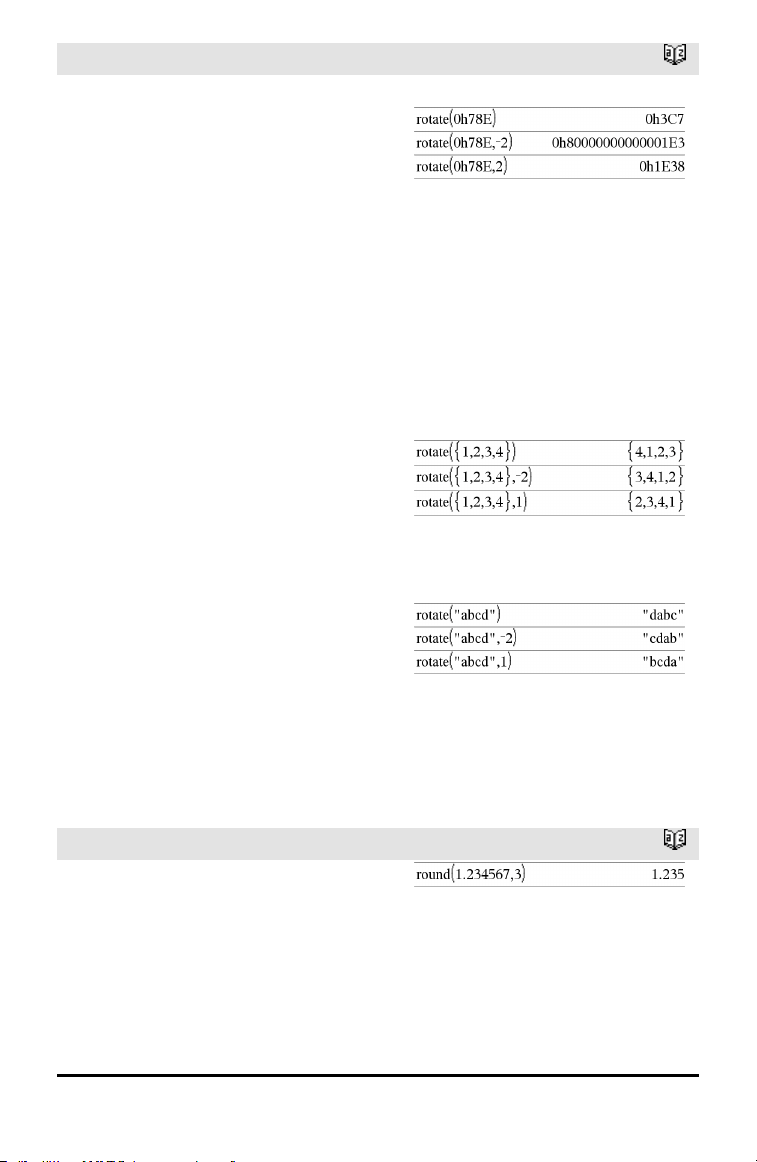
130 Alphabetical Listing
rotate()
Catalog >
If #ofRotations is positive, the rotation is to
the left. If #ofRotations is negative, the
rotation is to the right. The default is −1
(rotate right one bit).
For example, in a right rotation:
In Hex base mode:
Each bit rotates right.
0b00000000000001111010110000110101
Rightmost bit rotates to leftmost.
produces:
0b10000000000000111101011000011010
The result is displayed according to the
Base mode.
Important: To enter a binary or
hexadecimalnumber, always use the 0b or
0hprefix (zero, not the letter O).
rotate(List1[,#ofRotations]) ⇒ list
Returns a copy of List1 rotated right or left
by #of Rotations elements. Does not alter
List1.
If #ofRotations is positive, the rotation is to
the left. If #of Rotations is negative, the
rotation is to the right. The default is −1
(rotate right one element).
In Dec base mode:
rotate(String1[,#ofRotations]) ⇒ string
Returns a copy of String1 rotated right or
left by #ofRotations characters. Does not
alter String1.
If #ofRotations is positive, the rotation is to
the left. If #ofRotations is negative, the
rotation is to the right. The default is −1
(rotate right one character).
round()
Catalog >
round(Value1[, digits]) ⇒ value
Returns the argument rounded to the
specified number of digits after the decimal
point.
digits must be an integer in the range 0–
12. If digits is not included, returns the
argument rounded to 12 significant digits.
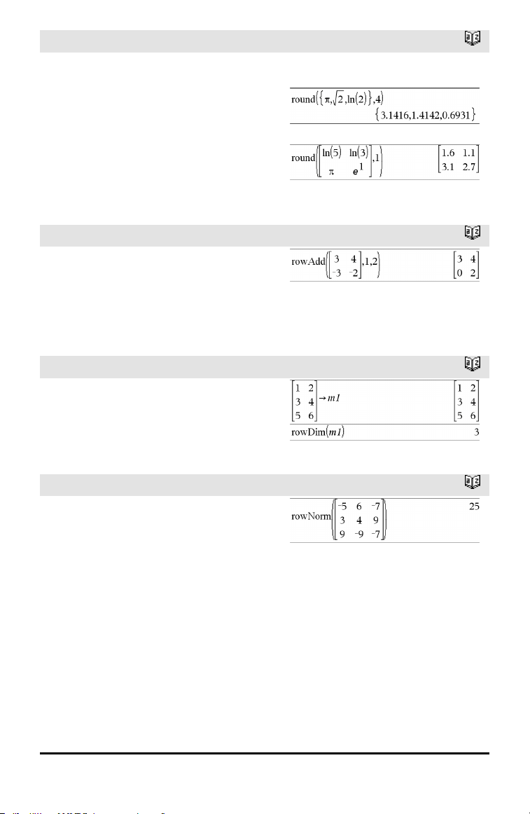
round()
Catalog >
Note: Display digits mode may affect how
this is displayed.
round(List1[, digits]) ⇒ list
Returns a list of the elements rounded to
the specified number of digits.
round(Matrix1[, digits]) ⇒ matrix
Returns a matrix of the elements rounded
to the specified number of digits.
rowAdd()
Catalog >
rowAdd(Matrix1, rIndex1, rIndex2) ⇒
matrix
Returns a copy of Matrix1 with row
rIndex2 replaced by the sum of rows
rIndex1 and rIndex2.
rowDim()
Catalog >
rowDim(Matrix) ⇒ expression
Returns the number of rows in Matrix.
Note: See also colDim(), page 23.
rowNorm()
Catalog >
rowNorm(Matrix) ⇒ expression
Returns the maximum of the sums of the
absolute values of the elements in the rows
in Matrix.
Note: All matrix elements must simplify to
numbers. See also colNorm(), page 23.
Alphabetical Listing 131
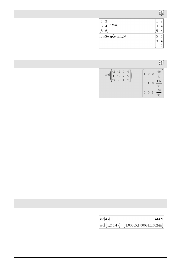
132 Alphabetical Listing
rowSwap()
Catalog >
rowSwap(Matrix1, rIndex1, rIndex2) ⇒
matrix
Returns Matrix1 with rows rIndex1 and
rIndex2 exchanged.
rref()
Catalog >
rref(Matrix1[, Tol]) ⇒ matrix
Returns the reduced row echelon form of
Matrix1.
Optionally, any matrix element is treated as
zero if its absolute value is less than Tol.
This tolerance is used only if the matrix has
floating-point entries and does not contain
any symbolic variables that have not been
assigned a value. Otherwise, Tol is ignored.
• If you use /· or set the Auto or
Approximate mode to Approximate,
computations are done using floating-
point arithmetic.
• If Tol is omitted or not used, the default
tolerance is calculated as:
5E−14 •max(dim(Matrix1)) •rowNorm
(Matrix1)
Note: See also ref(), page 122.
S
sec()
µ key
sec(Value1) ⇒ value
sec(List1) ⇒ list
Returns the secant of Value1 or returns a
list containing the secants of all elements
in List1.
In Degree angle mode:
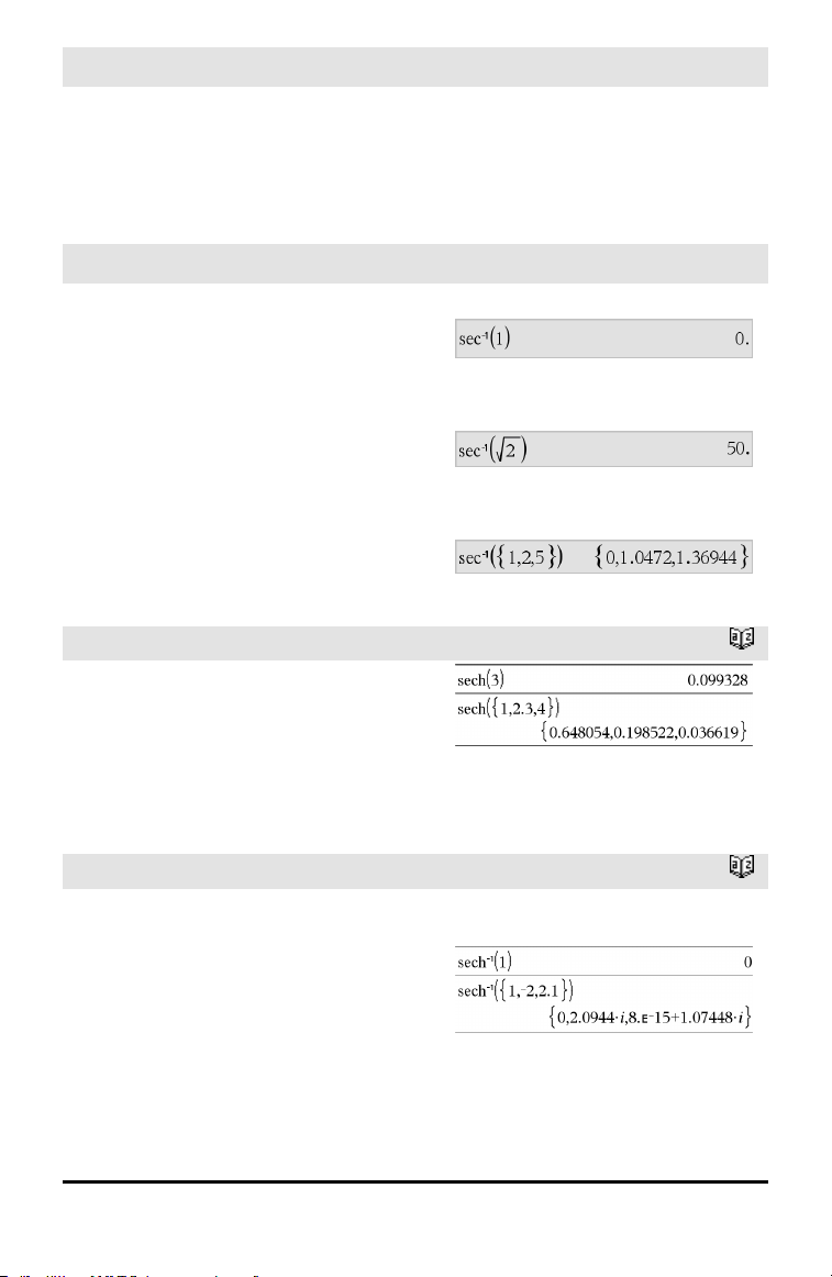
sec()
µ key
Note: The argument is interpreted as a
degree, gradian or radian angle, according
to the current angle mode setting. You can
use °,
G
, or
r
to override the angle mode
temporarily.
sec⁻¹()
µ key
sec⁻¹(Value1) ⇒ value
sec⁻¹(List1) ⇒ list
Returns the angle whose secant is Value1
or returns a list containing the inverse
secants of each element of List1.
Note: The result is returned as a degree,
gradian, or radian angle, according to the
current angle mode setting.
Note: You can insert this function from the
keyboard by typing arcsec(...).
In Degree angle mode:
In Gradian angle mode:
In Radian angle mode:
sech()
Catalog >
sech(Value1) ⇒ value
sech(List1) ⇒ list
Returns the hyperbolic secant of Value1 or
returns a list containing the hyperbolic
secants of the List1 elements.
sech⁻¹()
Catalog >
sech⁻¹(Value1) ⇒ value
sech⁻¹(List1) ⇒ list
Returns the inverse hyperbolic secant of
Value1 or returns a list containing the
inverse hyperbolic secants of each element
of List1.
Note: You can insert this function from the
keyboard by typing arcsech(...).
In Radian angle and Rectangular complex
mode:
Alphabetical Listing 133
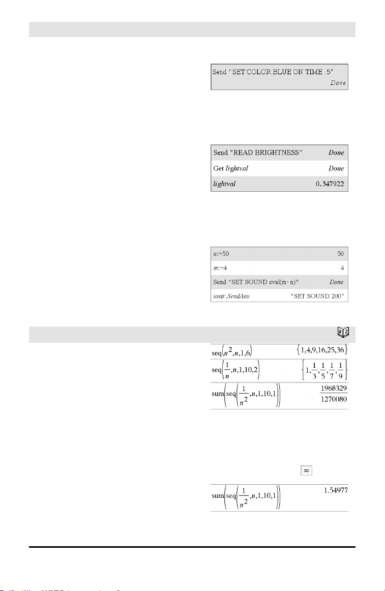
134 Alphabetical Listing
Send Hub Menu
Send exprOrString1 [, exprOrString2] ...
Programming command: Sends one or
more TI-Innovator™ Hub commands to a
connected hub.
exprOrString must be a valid TI-Innovator™
Hub Command. Typically, exprOrString
contains a "SET..." command to control a
device or a "READ..." command to request
data.
The arguments are sent to the hub in
succession.
Note: You can use the Send command
within a user-defined program but not
within a function.
Note: See also Get (page 58), GetStr (page
65), and eval() (page 47).
Example: Turn on the blue element of the
built-in RGB LED for 0.5 seconds.
Example: Request the current value of the
hub's built-in light-level sensor. A Get
command retrieves the value andassigns it
to variable lightval.
Example: Send a calculated frequency to the
hub's built-in speaker. Use special variable
iostr.SendAns to show the hubcommand
withthe expression evaluated.
seq()
Catalog >
seq(Expr, Var, Low, High[, Step]) ⇒ list
Increments Var from Low through High by
an increment of Step, evaluates Expr, and
returns the results as a list. The original
contents of Var are still there after seq() is
completed.
The default value for Step = 1.
Note: To force an approximate result,
Handheld: Press / ·.
Windows®: Press Ctrl+Enter.
Macintosh®: Press “+Enter.
iPad®: Holdenter, and select .
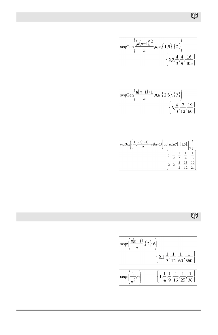
seqGen()
Catalog >
seqGen(Expr, Var, depVar, {Var0,
VarMax}[, ListOfInitTerms
[, VarStep[, CeilingValue]]]) ⇒ list
Generates a list of terms for sequence
depVar(Var)=Expr as follows: Increments
independent variable Var from Var0
through VarMax by VarStep, evaluates
depVar(Var) for corresponding values of
Var using the Expr formula and
ListOfInitTerms, and returns the results as
a list.
seqGen(ListOrSystemOfExpr, Var,
ListOfDepVars, {Var0, VarMax} [
, MatrixOfInitTerms[, VarStep[,
CeilingValue]]]) ⇒ matrix
Generates a matrix of terms for a system
(or list) of sequences ListOfDepVars(Var)
=ListOrSystemOfExpr as follows:
Increments independent variable Var from
Var0 through VarMax by VarStep,
evaluates ListOfDepVars(Var) for
corresponding values of Var using
ListOrSystemOfExpr formula and
MatrixOfInitTerms, and returns the results
as a matrix.
The original contents of Var are unchanged
after seqGen() is completed.
The default value for VarStep = 1.
Generate the first 5 terms of the sequence u
(n) = u(n-1)
2
/2, with u(1)=2 andVarStep=1.
Example inwhichVar0=2:
System of two sequences:
Note: The Void(_) in the initialterm matrix
above is usedto indicate thatthe initial term
for u1(n) is calculated using the explicit
sequence formula u1(n)=1/n.
seqn()
Catalog >
seqn(Expr(u, n[, ListOfInitTerms[, nMax[,
CeilingValue]]]) ⇒ list
Generates a list of terms for a sequence u
(n)=Expr(u, n) as follows: Increments n
from 1 through nMax by 1, evaluates u(n)
for corresponding values of n using the
Expr(u, n) formula and ListOfInitTerms,
and returns the results as a list.
seqn(Expr(n[, nMax[, CeilingValue]]) ⇒
list
Generate the first 6 terms of the sequence u
(n) = u(n-1)/2, withu(1)=2.
Alphabetical Listing 135
136 Alphabetical Listing
seqn()
Catalog >
Generates a list of terms for a non-
recursive sequence u(n)=Expr(n) as
follows: Increments n from 1 through nMax
by 1, evaluates u(n) for corresponding
values of n using the Expr(n) formula, and
returns the results as a list.
If nMax is missing, nMax is set to 2500
If nMax=0, nMax is set to 2500
Note: seqn() calls seqGen() with n0=1 and
nstep =1
setMode()
Catalog >
setMode(modeNameInteger,
settingInteger) ⇒ integer
setMode(list) ⇒ integer list
Valid only within a function or program.
setMode(modeNameInteger,
settingInteger) temporarily sets mode
modeNameInteger to the new setting
settingInteger, and returns an integer
corresponding to the original setting of that
mode. The change is limited to the duration
of the program/function’s execution.
modeNameInteger specifies which mode
you want to set. It must be one of the mode
integers from the table below.
settingInteger specifies the new setting for
the mode. It must be one of the setting
integers listed below for the specific mode
you are setting.
setMode(list) lets you change multiple
settings. list contains pairs of mode
integers and setting integers. setMode(list)
returns a similar list whose integer pairs
represent the original modes and settings.
If you have saved all mode settings with
getMode(0)→var, you can use setMode
(var) to restore those settings until the
function or program exits. See getMode(),
page 64.
Display approximate value of π using the
default setting for Display Digits, and then
display π with a setting of Fix2. Check to see
that the default is restored after the
program executes.

setMode()
Catalog >
Note: The current mode settings are passed
to called subroutines. If any subroutine
changes a mode setting, the mode change
will be lost when control returns to the
calling routine.
Note for entering the example: For
instructions on entering multi-line program
and function definitions, refer to the
Calculator section of your product
guidebook.
Mode
Name
Mode
Integer Setting Integers
Display
Digits
1
1=Float, 2=Float1, 3=Float2, 4=Float3, 5=Float4, 6=Float5,
7=Float6, 8=Float7, 9=Float8, 10=Float9, 11=Float10,
12=Float11, 13=Float12, 14=Fix0, 15=Fix1, 16=Fix2,
17=Fix3, 18=Fix4, 19=Fix5, 20=Fix6, 21=Fix7, 22=Fix8,
23=Fix9, 24=Fix10, 25=Fix11, 26=Fix12
Angle
2
1=Radian, 2=Degree, 3=Gradian
Exponential
Format
3
1=Normal, 2=Scientific, 3=Engineering
Real or
Complex
4
1=Real, 2=Rectangular, 3=Polar
Auto or
Approx.
5
1=Auto, 2=Approximate
Vector
Format
6
1=Rectangular, 2=Cylindrical, 3=Spherical
Base
7
1=Decimal, 2=Hex, 3=Binary
shift()
Catalog >
shift(Integer1[,#ofShifts]) ⇒ integer
Shifts the bits in a binary integer. You can
enter Integer1 in any number base; it is
converted automatically to a signed, 64-bit
binary form. If the magnitude of Integer1 is
too large for this form, a symmetric modulo
operation brings it within the range. For
more information, see ►Base2, page 16.
In Bin base mode:
In Hex base mode:
Alphabetical Listing 137
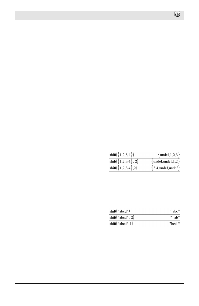
138 Alphabetical Listing
shift()
Catalog >
If #ofShifts is positive, the shift is to the
left. If #ofShifts is negative, the shift is to
the right. The default is −1 (shift right one
bit).
In a right shift, the rightmost bit is dropped
and 0 or 1 is inserted to match the leftmost
bit. In a left shift, the leftmost bit is
dropped and 0 is inserted as the rightmost
bit.
For example, in a right shift:
Each bit shifts right.
0b0000000000000111101011000011010
Inserts 0 if leftmost bit is 0,
or 1 if leftmost bit is 1.
produces:
0b00000000000000111101011000011010
The result is displayed according to the
Base mode. Leading zeros are not shown.
Important: To enter a binary or
hexadecimalnumber, always use the 0b or
0hprefix (zero, not the letter O).
shift(List1[,#ofShifts]) ⇒ list
Returns a copy of List1 shifted right or left
by #ofShifts elements. Does not alter List1.
If #ofShifts is positive, the shift is to the
left. If #ofShifts is negative, the shift is to
the right. The default is −1 (shift right one
element).
Elements introduced at the beginning or
end of list by the shift are set to the symbol
“undef”.
In Dec base mode:
shift(String1[,#ofShifts]) ⇒ string
Returns a copy of String1 shifted right or
left by #ofShifts characters. Does not alter
String1.
If #ofShifts is positive, the shift is to the
left. If #ofShifts is negative, the shift is to
the right. The default is −1 (shift right one
character).
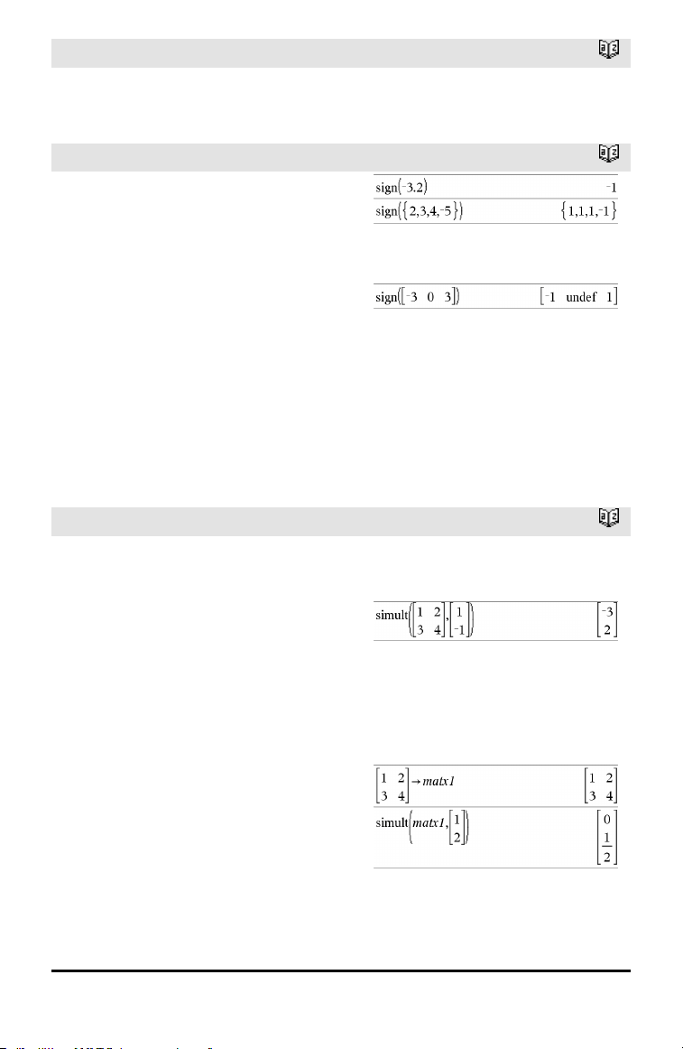
shift()
Catalog >
Characters introduced at the beginning or
end of string by the shift are set to a space.
sign()
Catalog >
sign(Value1) ⇒ value
sign(List1) ⇒ list
sign(Matrix1) ⇒ matrix
For real and complex Value1, returns
Value1/abs(Value1) when Value1 ≠ 0.
Returns 1 if Value1is positive.Returns −1 if
Value1 is negative. sign(0) returns „1 if the
complex format mode is Real; otherwise, it
returns itself.
sign(0) represents the unit circle in the
complex domain.
For a list or matrix, returns the signs of all
the elements.
If complex formatmode is Real:
simult()
Catalog >
simult(coeffMatrix, constVector[, Tol]) ⇒
matrix
Returns a column vector that contains the
solutions to a system of linear equations.
Note: See also linSolve(), page 81.
coeffMatrix must be a square matrix that
contains the coefficients of the equations.
constVector must have the same number
of rows (same dimension) as coeffMatrix
and contain the constants.
Optionally, any matrix element is treated as
zero if its absolute value is less than Tol.
This tolerance is used only if the matrix has
floating-point entries and does not contain
any symbolic variables that have not been
assigned a value. Otherwise, Tol is ignored.
• If you set the Auto or Approximate mode
to Approximate, computations are done
Solve for x andy:
x + 2y = 1
3x + 4y = −1
The solution is x=−3 and y=2.
Solve:
ax + by = 1
cx + dy = 2
Alphabetical Listing 139
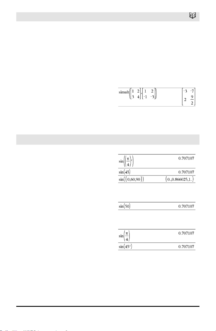
140 Alphabetical Listing
simult()
Catalog >
using floating-point arithmetic.
• If Tol is omitted or not used, the default
tolerance is calculated as:
5E−14 •max(dim(coeffMatrix))
•rowNorm(coeffMatrix)
simult(coeffMatrix, constMatrix[, Tol]) ⇒
matrix
Solves multiple systems of linear equations,
where each system has the same equation
coefficients but different constants.
Each column in constMatrix must contain
the constants for a system of equations.
Each column in the resulting matrix
contains the solution for the corresponding
system.
Solve:
x + 2y = 1
3x + 4y = −1
x + 2y = 2
3x + 4y = −3
For the first system, x=−3 and y=2. For the
second system, x=−7 and y=9/2.
sin()
µ key
sin(Value1) ⇒ value
sin(List1) ⇒ list
sin(Value1) returns the sine of the
argument.
sin(List1) returns a list of the sines of all
elements in List1.
Note: The argument is interpreted as a
degree, gradian or radian angle, according
to the current angle mode. You can use°,
g
,
or
r
to override the angle mode setting
temporarily.
In Degree angle mode:
In Gradian angle mode:
In Radian angle mode:
sin(squareMatrix1) ⇒ squareMatrix
Returns the matrix sine of squareMatrix1.
This is not the same as calculating the sine
of each element. For information about the
calculation method, refer to cos().
In Radian angle mode:
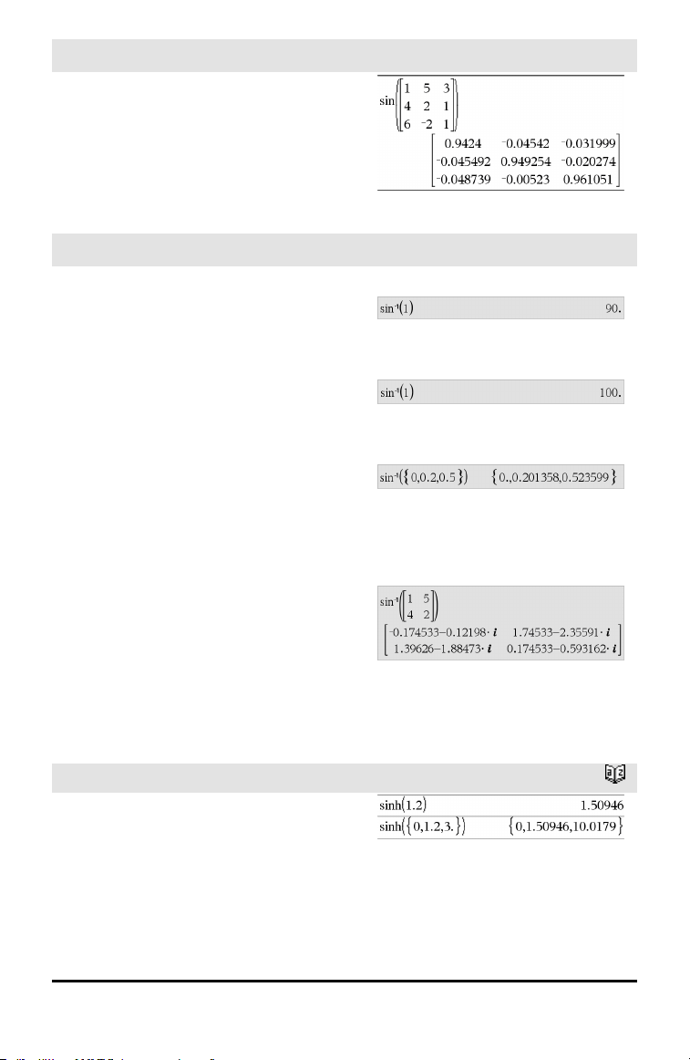
sin()
µ key
squareMatrix1 must be diagonalizable. The
result always contains floating-point
numbers.
sin⁻¹()
µ key
sin⁻¹(Value1) ⇒ value
sin⁻¹(List1) ⇒ list
sin⁻¹(Value1) returns the angle whose sine
is Value1.
sin⁻¹(List1) returns a list of the inverse
sines of each element of List1.
Note: The result is returned as a degree,
gradian or radian angle, according to the
current angle mode setting.
Note: You can insert this function from the
keyboard by typing arcsin(...).
In Degree angle mode:
In Gradian angle mode:
In Radian angle mode:
sin⁻¹(squareMatrix1) ⇒ squareMatrix
Returns the matrix inverse sine of
squareMatrix1. This is not the same as
calculating the inverse sine of each
element. For information about the
calculation method, refer to cos().
squareMatrix1 must be diagonalizable. The
result always contains floating-point
numbers.
In Radian angle mode and Rectangular
complex format mode:
sinh()
Catalog >
sinh(Numver1) ⇒ value
sinh(List1) ⇒ list
sinh (Value1) returns the hyperbolic sine of
the argument.
sinh (List1) returns a list of the hyperbolic
sines of each element of List1.
Alphabetical Listing 141
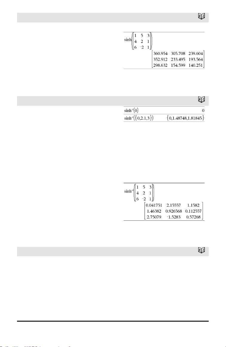
142 Alphabetical Listing
sinh()
Catalog >
sinh(squareMatrix1) ⇒ squareMatrix
Returns the matrix hyperbolic sine of
squareMatrix1. This is not the same as
calculating the hyperbolic sine of each
element. For information about the
calculation method, refer to cos().
squareMatrix1 must be diagonalizable. The
result always contains floating-point
numbers.
In Radian angle mode:
sinh⁻¹()
Catalog >
sinh⁻¹(Value1) ⇒ value
sinh⁻¹(List1) ⇒ list
sinh⁻¹(Value1) returns the inverse
hyperbolic sine of the argument.
sinh⁻¹(List1) returns a list of the inverse
hyperbolic sines of each element of List1.
Note: You can insert this function from the
keyboard by typing arcsinh(...).
sinh⁻¹(squareMatrix1) ⇒ squareMatrix
Returns the matrix inverse hyperbolic sine
of squareMatrix1. This is not the same as
calculating the inverse hyperbolic sine of
each element. For information about the
calculation method, refer to cos().
squareMatrix1 must be diagonalizable. The
result always contains floating-point
numbers.
In Radian angle mode:
SinReg
Catalog >
SinReg X, Y[, [Iterations],[Period][,
Category, Include]]
Computes the sinusoidal regression on lists
X and Y. A summary of results is stored in
the stat.results variable. (See page 145.)
All the lists must have equal dimension
except for Include.

SinReg
Catalog >
X and Y are lists of independent and
dependent variables.
Iterations is a value that specifies the
maximum number of times (1 through 16) a
solution will be attempted. If omitted, 8 is
used. Typically, larger values result in better
accuracy but longer execution times, and
vice versa.
Period specifies an estimated period. If
omitted, the difference between values in X
should be equal and in sequential order. If
you specify Period, the differences between
x values can be unequal.
Category is a list of numeric or string
category codes for the corresponding X and
Y data.
Include is a list of one or more of the
category codes. Only those data items
whose category code is included in this list
are included in the calculation.
The output of SinReg is always in radians,
regardless of the angle mode setting.
For information on the effect of empty
elements in a list, see “Empty (Void)
Elements,” page 196.
Output
variable
Description
stat.RegEqn
Regression Equation: a•sin(bx+c)+d
stat.a, stat.b,
stat.c, stat.d
Regression coefficients
stat.Resid Residuals from the regression
stat.XReg
Listof data points in the modifiedX List actually used in the regression based on
restrictions of Freq, Category List, and Include Categories
stat.YReg
Listof data points in the modifiedY List actually used inthe regression basedon
restrictions of Freq, Category List, and Include Categories
stat.FreqReg
Listof frequencies corresponding to stat.XReg and stat.YReg
Alphabetical Listing 143
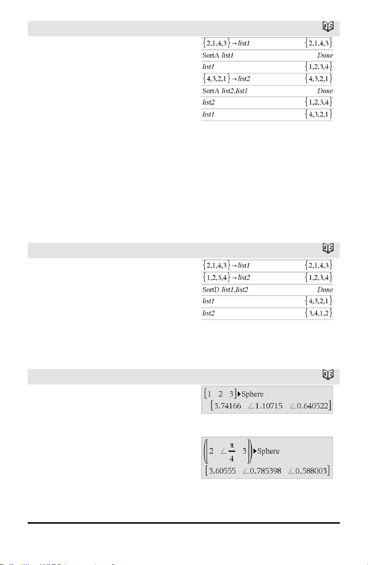
144 Alphabetical Listing
SortA
Catalog >
SortA List1[, List2] [, List3]...
SortA Vector1[, Vector2] [, Vector3]...
Sorts the elements of the first argument in
ascending order.
If you include additional arguments, sorts
the elements of each so that their new
positions match the new positions of the
elements in the first argument.
All arguments must be names of lists or
vectors. All arguments must have equal
dimensions.
Empty (void) elements within the first
argument move to the bottom. For more
information on empty elements, see page
196.
SortD
Catalog >
SortD List1[, List2][, List3]...
SortD Vector1[,Vector2][,Vector3]...
Identical to SortA, except SortD sorts the
elements in descending order.
Empty (void) elements within the first
argument move to the bottom. For more
information on empty elements, see page
196.
►Sphere
Catalog >
Vector►Sphere
Note: You can insert this operator from the
computer keyboard by typing @>Sphere.
Displays the row or column vector in
spherical form [ρ∠θ∠φ].
Vector must be of dimension 3 and can be
either a row or a column vector.
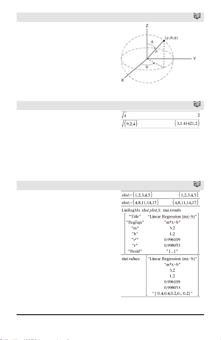
►Sphere
Catalog >
Note: ►Sphere is a display-format
instruction, not a conversion function. You
can use it only at the end of an entry line.
sqrt()
Catalog >
sqrt(Value1) ⇒ value
sqrt(List1) ⇒ list
Returns the square root of the argument.
For a list, returns the square roots of all the
elements in List1.
Note: See also Square root template, page
1.
stat.results
Catalog >
stat.results
Displays results from a statistics
calculation.
The results are displayed as a set of name-
value pairs. The specific names shown are
dependent on the most recently evaluated
statistics function or command.
You can copy a name or value and paste it
into other locations.
Note: Avoid defining variables that use the
same names as those used for statistical
analysis. In some cases, an error condition
could occur. Variable names used for
statistical analysis are listed in the table
below.
Alphabetical Listing 145

146 Alphabetical Listing
stat.a
stat.AdjR²
stat.b
stat.b0
stat.b1
stat.b2
stat.b3
stat.b4
stat.b5
stat.b6
stat.b7
stat.b8
stat.b9
stat.b10
stat.bList
stat.χ²
stat.c
stat.CLower
stat.CLowerList
stat.CompList
stat.CompMatrix
stat.CookDist
stat.CUpper
stat.CUpperList
stat.d
stat.dfDenom
stat.dfBlock
stat.dfCol
stat.dfError
stat.dfInteract
stat.dfReg
stat.dfNumer
stat.dfRow
stat.DW
stat.e
stat.ExpMatrix
stat.F
stat.FBlock
stat.Fcol
stat.FInteract
stat.FreqReg
stat.Frow
stat.Leverage
stat.LowerPred
stat.LowerVal
stat.m
stat.MaxX
stat.MaxY
stat.ME
stat.MedianX
stat.MedianY
stat.MEPred
stat.MinX
stat.MinY
stat.MS
stat.MSBlock
stat.MSCol
stat.MSError
stat.MSInteract
stat.MSReg
stat.MSRow
stat.n
Stat.Ç
stat.Ç1
stat.Ç2
stat.ÇDiff
stat.PList
stat.PVal
stat.PValBlock
stat.PValCol
stat.PValInteract
stat.PValRow
stat.Q1X
stat.Q1Y
stat.Q3X
stat.Q3Y
stat.r
stat.r²
stat.RegEqn
stat.Resid
stat.ResidTrans
stat.σx
stat.σy
stat.σx1
stat.σx2
stat.Σx
stat.Σx²
stat.Σxy
stat.Σy
stat.Σy²
stat.s
stat.SE
stat.SEList
stat.SEPred
stat.sResid
stat.SEslope
stat.sp
stat.SS
stat.SSBlock
stat.SSCol
stat.SSX
stat.SSY
stat.SSError
stat.SSInteract
stat.SSReg
stat.SSRow
stat.tList
stat.UpperPred
stat.UpperVal
stat.v
stat.v1
stat.v2
stat.vDiff
stat.vList
stat.XReg
stat.XVal
stat.XValList
stat.w
stat.y
stat.yList
stat.YReg
Note: Each time the Lists & Spreadsheet application calculates statistical results, it
copies the “stat.” group variables to a “stat#.” group, where # is a number that is
incremented automatically. This lets you maintain previous results while
performing multiple calculations.
stat.values
Catalog >
stat.values
Displays a matrix of the values calculated for
the most recently evaluated statistics
function or command.
Unlike stat.results, stat.values omits the
names associated with the values.
You can copy a value and paste it into other
locations.
See the stat.results example.
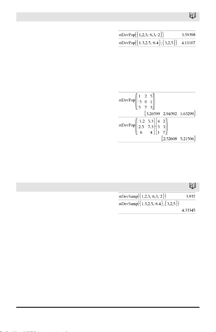
stDevPop()
Catalog >
stDevPop(List [, freqList]) ⇒ expression
Returns the population standard deviation
of the elements in List.
Each freqList element counts the number
of consecutive occurrences of the
corresponding element in List.
Note:List must have at least two elements.
Empty (void) elements are ignored. For
more information on empty elements, see
page 196.
In Radian angle and auto modes:
stDevPop(Matrix1[, freqMatrix]) ⇒
matrix
Returns a row vector of the population
standard deviations of the columns in
Matrix1.
Each freqMatrix element counts the
number of consecutive occurrences of the
corresponding element in Matrix1.
Note:Matrix1must have at least two rows.
Empty (void) elements are ignored. For
more information on empty elements, see
page 196.
stDevSamp()
Catalog >
stDevSamp(List[, freqList]) ⇒ expression
Returns the sample standard deviation of
the elements in List.
Each freqList element counts the number
of consecutive occurrences of the
corresponding element in List.
Note:List must have at least two elements.
Empty (void) elements are ignored. For
more information on empty elements, see
page 196.
Alphabetical Listing 147
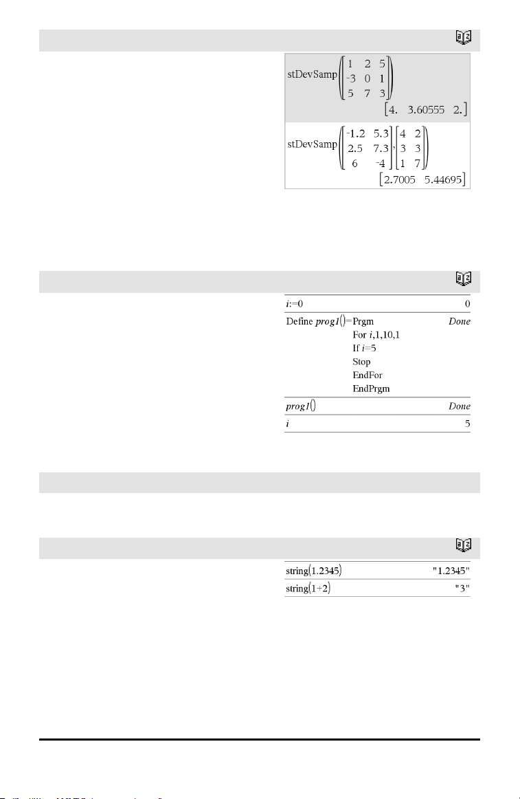
148 Alphabetical Listing
stDevSamp()
Catalog >
stDevSamp(Matrix1[, freqMatrix]) ⇒
matrix
Returns a row vector of the sample
standard deviations of the columns in
Matrix1.
Each freqMatrix element counts the
number of consecutive occurrences of the
corresponding element in Matrix1.
Note:Matrix1must have at least two rows.
Empty (void) elements are ignored. For
more information on empty elements, see
page 196.
Stop
Catalog >
Stop
Programming command: Terminates the
program.
Stop is not allowed in functions.
Note for entering the example: For
instructions on entering multi-line program
and function definitions, refer to the
Calculator section of your product
guidebook.
Store
See →(store), page 193.
string()
Catalog >
string(Expr) ⇒ string
Simplifies Expr and returns the result as a
character string.
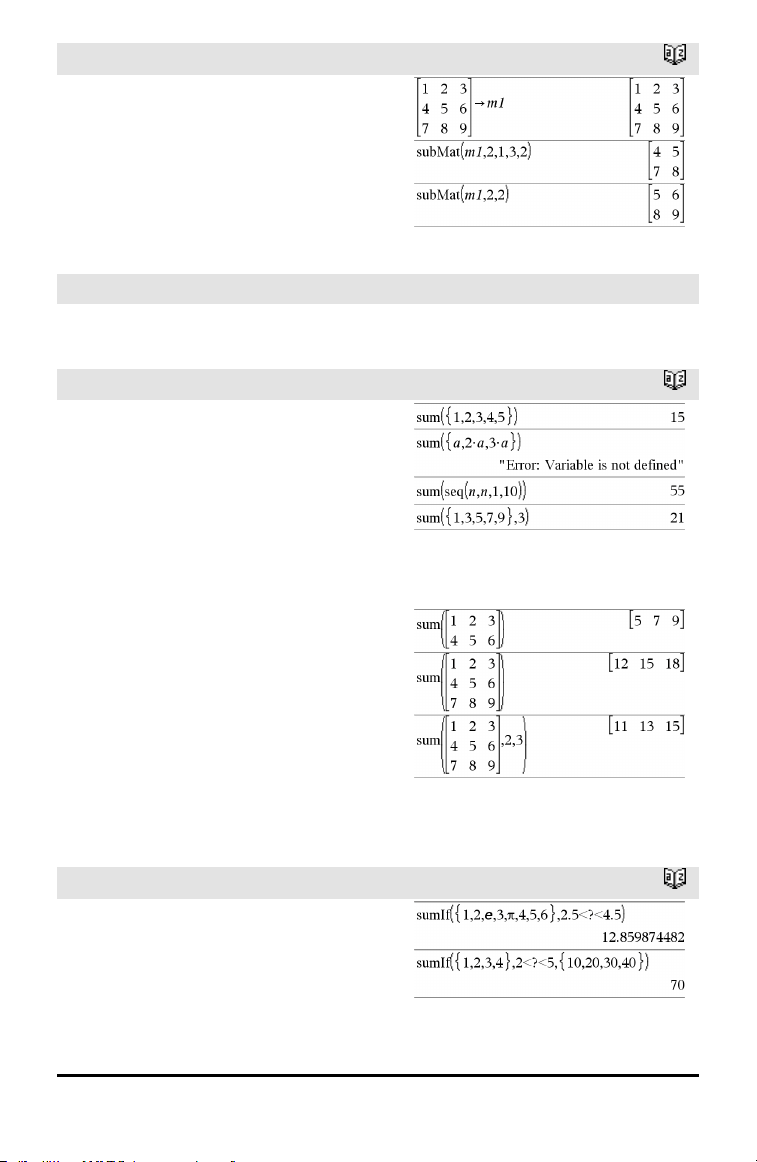
subMat()
Catalog >
subMat(Matrix1[, startRow][, startCol][,
endRow][, endCol]) ⇒ matrix
Returns the specified submatrix of Matrix1.
Defaults: startRow=1, startCol=1,
endRow=last row, endCol=last column.
Sum (Sigma)
See Σ(), page 186.
sum()
Catalog >
sum(List[, Start[, End]]) ⇒ expression
Returns the sum of all elements in List.
Start and End are optional. They specify a
range of elements.
Any void argument produces a void result.
Empty (void) elements in List are ignored.
For more information on empty elements,
see page 196.
sum(Matrix1[, Start[, End]]) ⇒ matrix
Returns a row vector containing the sums
of all elements in the columns in Matrix1.
Start and End are optional. They specify a
range of rows.
Any void argument produces a void result.
Empty (void) elements in Matrix1 are
ignored. For more information on empty
elements, see page 196.
sumIf()
Catalog >
sumIf(List,Criteria[, SumList]) ⇒ value
Returns the accumulated sum of all
elements in List that meet the specified
Criteria. Optionally, you can specify an
alternate list, sumList, to supply the
elements to accumulate.
Alphabetical Listing 149

150 Alphabetical Listing
sumIf()
Catalog >
List can be an expression, list, or matrix.
SumList, if specified, must have the same
dimension(s) as List.
Criteria can be:
• A value, expression, or string. For
example, 34 accumulates only those
elements in List that simplify to the
value 34.
• A Boolean expression containing the
symbol ? as a placeholder for each
element. For example, ?<10 accumulates
only those elements in List that are less
than 10.
When a List element meets the Criteria,
the element is added to the accumulating
sum. If you include sumList, the
corresponding element from sumList is
added to the sum instead.
Within the Lists & Spreadsheet application,
you can use a range of cells in place of List
and sumList.
Empty (void) elements are ignored. For
more information on empty elements, see
page 196.
Note: See also countIf(), page 29.
sumSeq()
See Σ(), page 186.
system()
Catalog >
system(Value1[, Value2[, Value3[, ...]]])
Returns a system of equations, formatted as
a list. You can also create a system by using
a template.
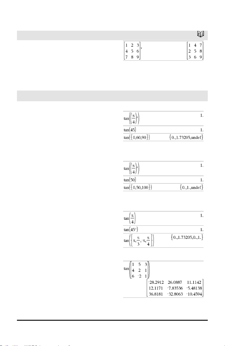
T
T (transpose)
Catalog >
Matrix1T ⇒ matrix
Returns the complex conjugate transpose of
Matrix1.
Note: You can insert this operator from the
computer keyboard by typing @t.
tan()
µ key
tan(Value1) ⇒ value
tan(List1) ⇒ list
tan(Value1) returns the tangent of the
argument.
tan(List1) returns a list of the tangents of
all elements in List1.
Note: The argument is interpreted as a
degree, gradian or radian angle, according
to the current angle mode. You can use°,
g
or
r
to override the angle mode setting
temporarily.
In Degree angle mode:
In Gradian angle mode:
In Radian angle mode:
tan(squareMatrix1) ⇒ squareMatrix
Returns the matrix tangent of
squareMatrix1. This is not the same as
calculating the tangent of each element.
For information about the calculation
method, refer to cos().
In Radian angle mode:
Alphabetical Listing 151
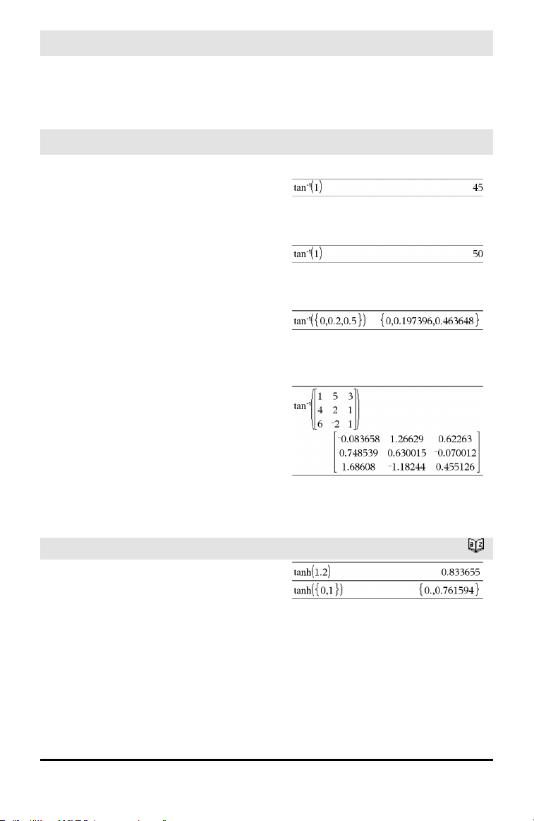
152 Alphabetical Listing
tan()
µ key
squareMatrix1 must be diagonalizable. The
result always contains floating-point
numbers.
tan⁻¹()
µ key
tan⁻¹(Value1) ⇒ value
tan⁻¹(List1) ⇒ list
tan⁻¹(Value1) returns the angle whose
tangent is Value1.
tan⁻¹(List1) returns a list of the inverse
tangents of each element of List1.
Note: The result is returned as a degree,
gradian or radian angle, according to the
current angle mode setting.
Note: You can insert this function from the
keyboard by typing arctan(...).
In Degree angle mode:
In Gradian angle mode:
In Radian angle mode:
tan⁻¹(squareMatrix1) ⇒ squareMatrix
Returns the matrix inverse tangent of
squareMatrix1. This is not the same as
calculating the inverse tangent of each
element. For information about the
calculation method, refer to cos().
squareMatrix1 must be diagonalizable. The
result always contains floating-point
numbers.
In Radian angle mode:
tanh()
Catalog >
tanh(Value1) ⇒ value
tanh(List1) ⇒ list
tanh(Value1) returns the hyperbolic
tangent of the argument.
tanh(List1) returns a list of the hyperbolic
tangents of each element of List1.
tanh(squareMatrix1) ⇒ squareMatrix
In Radian angle mode:
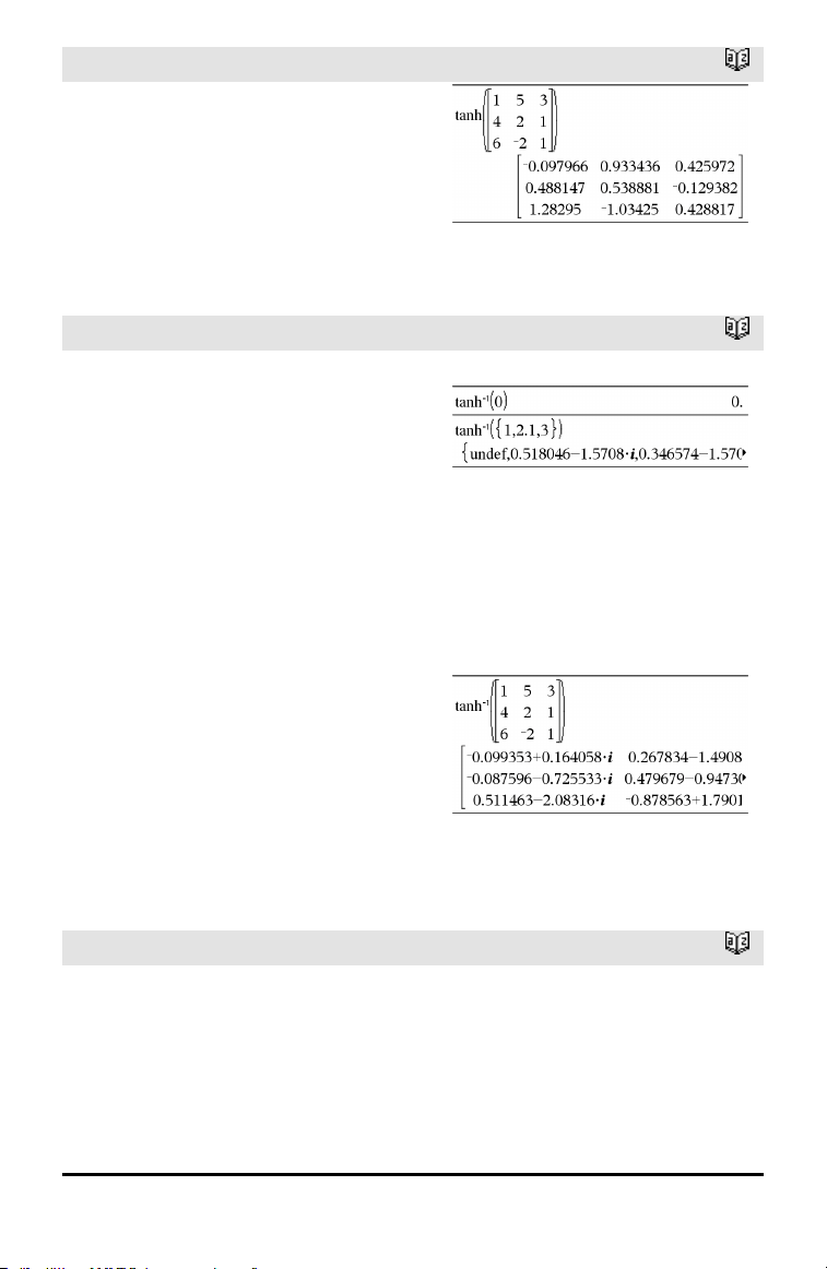
tanh()
Catalog >
Returns the matrix hyperbolic tangent of
squareMatrix1. This is not the same as
calculating the hyperbolic tangent of each
element. For information about the
calculation method, refer to cos().
squareMatrix1 must be diagonalizable. The
result always contains floating-point
numbers.
tanh⁻¹()
Catalog >
tanh⁻¹(Value1) ⇒ value
tanh⁻¹(List1) ⇒ list
tanh⁻¹(Value1) returns the inverse
hyperbolic tangent of the argument.
tanh⁻¹(List1) returns a list of the inverse
hyperbolic tangents of each element of
List1.
Note: You can insert this function from the
keyboard by typing arctanh(...).
In Rectangular complex format:
To see the entire result, press £ and then
use ¡and¢ to move the cursor.
tanh⁻¹(squareMatrix1) ⇒ squareMatrix
Returns the matrix inverse hyperbolic
tangent of squareMatrix1. This is not the
same as calculating the inverse hyperbolic
tangent of each element. For information
about the calculation method, refer to cos
().
squareMatrix1 must be diagonalizable. The
result always contains floating-point
numbers.
In Radian angle mode and Rectangular
complex format:
To see the entire result, press £ and then
use ¡and¢ to move the cursor.
tCdf()
Catalog >
tCdf(lowBound,upBound,df) ⇒ number if
lowBound and upBound are numbers, list if
lowBound and upBound are lists
Computes the Student-t distribution
probability between lowBound and upBound
for the specified degrees of freedom df.
Alphabetical Listing 153

154 Alphabetical Listing
tCdf()
Catalog >
For P(X ≤ upBound), set lowBound = ⁻9E999.
Text
Catalog >
TextpromptString[, DispFlag]
Programming command: Pauses the
program and displays the character string
promptString in a dialog box.
When the user selects OK, program
execution continues.
The optional flag argument can be any
expression.
• If DispFlag is omitted or evaluates to 1,
the text message is added to the
Calculator history.
• If DispFlag evaluates to 0, the text
message is not added to the history.
If the program needs a typed response from
the user, refer to Request, page 125, or
RequestStr, page 126.
Note: You can use this command within a
user-defined program but not within a
function.
Define a program that pauses to display
each of five random numbers ina dialog
box.
Within the Prgm...EndPrgm template,
complete eachline by pressing @ instead
of ·. On the computer keyboard, hold
down Alt and press Enter.
Define text_demo()=Prgm
For i,1,5
strinfo:=”Random number “&
string(rand(i))
Text strinfo
EndFor
EndPrgm
Run the program:
text_demo()
Sample of one dialog box:
Then
See If, page 67.
tInterval
Catalog >
tInterval List[, Freq[, CLevel]]
(Data list input)
tInterval v, sx, n[, CLevel]
(Summary stats input)

tInterval
Catalog >
Computes a t confidence interval. A
summary of results is stored in the
stat.results variable. (See page 145.)
For information on the effect of empty
elements in a list, see “Empty (Void)
Elements,” page 196.
Output variable Description
stat.CLower, stat.CUpper Confidence interval for an unknown population mean
stat.v Sample mean of the data sequence from the normal random distribution
stat.ME Marginof error
stat.df Degrees of freedom
stat.σx
Sample standard deviation
stat.n Length of the data sequence with sample mean
tInterval_2Samp
Catalog >
tInterval_2Samp List1,List2[,Freq1[,Freq2
[,CLevel[,Pooled]]]]
(Data list input)
tInterval_2Samp v1,sx1,n1,v2,sx2,n2
[,CLevel[,Pooled]]
(Summary stats input)
Computes a two-sample t confidence
interval. A summary of results is stored in
the stat.results variable. (See page 145.)
Pooled=1 pools variances; Pooled=0 does
not pool variances.
For information on the effect of empty
elements in a list, see “Empty (Void)
Elements,” page 196.
Output variable Description
stat.CLower,
stat.CUpper
Confidence interval containing confidence levelprobability of distribution
stat.v1-v2 Sample means of the data sequences from the normal random
distribution
Alphabetical Listing 155
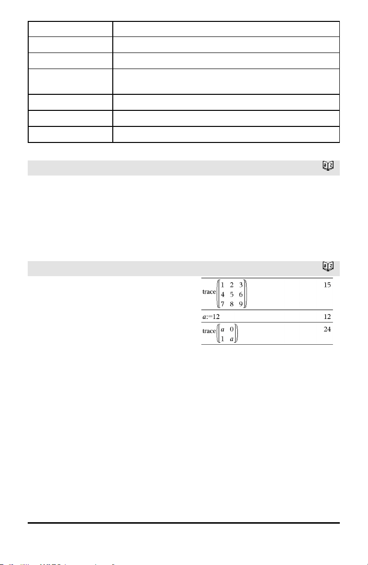
156 Alphabetical Listing
Output variable Description
stat.ME Margin of error
stat.df Degrees of freedom
stat.v1, stat.v2 Sample means of the data sequences from the normal random
distribution
stat.σx1, stat.σx2 Sample standard deviations for List 1 and List 2
stat.n1, stat.n2 Number of samples indata sequences
stat.sp
The pooled standard deviation. Calculated when Pooled=YES
tPdf()
Catalog >
tPdf(XVal,df) ⇒ number if XVal is a
number, list if XVal is a list
Computes the probability density function
(pdf) for the Student-t distribution at a
specified x value with specified degrees of
freedom df.
trace()
Catalog >
trace(squareMatrix) ⇒ value
Returns the trace (sum of all the elements
on the main diagonal) of squareMatrix.
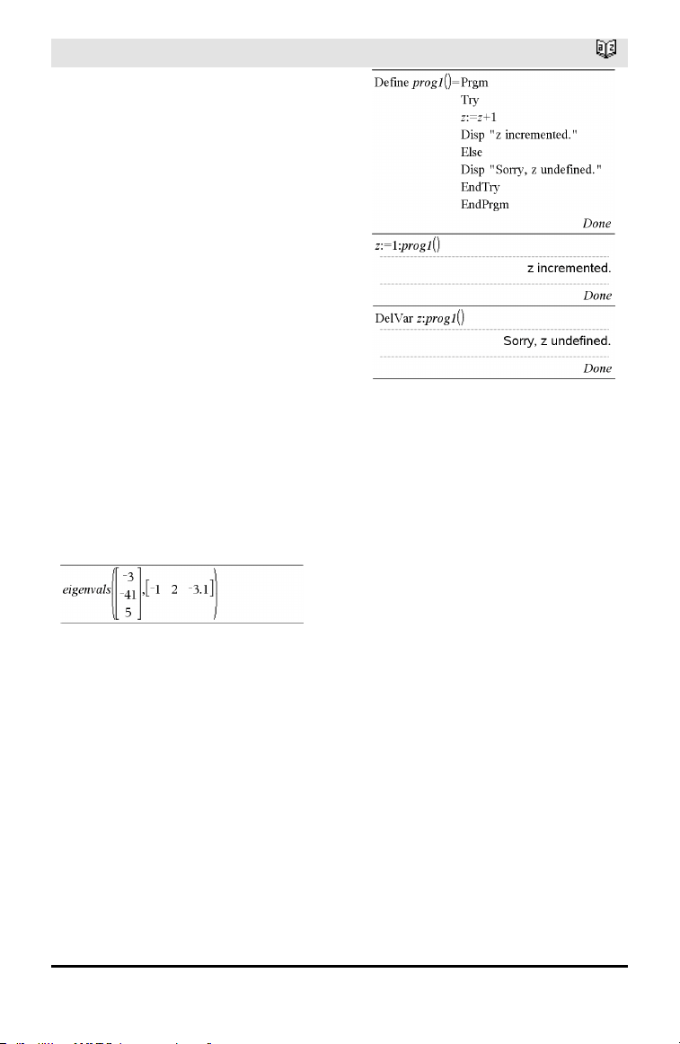
Try
Catalog >
Try
block1
Else
block2
EndTry
Executes block1 unless an error occurs.
Program execution transfers to block2 if an
error occurs in block1. System variable
errCode contains the error code to allow
the program to perform error recovery. For
a list of error codes, see “Error codes and
messages,” page 211.
block1 and block2 can be either a single
statement or a series of statements
separated with the “:” character.
Note for entering the example: For
instructions on entering multi-line program
and function definitions, refer to the
Calculator section of your product
guidebook.
To see the commands Try, ClrErr, and
PassErr in operation, enter the eigenvals()
program shown at the right. Run the
program by executing each of the following
expressions.
Note: See also ClrErr, page 22, and PassErr,
page 109.
Define eigenvals(a,b)=Prgm
© Program eigenvals(A,B) displays
eigenvalues of A•B
Try
Disp "A= ",a
Disp "B= ",b
Disp " "
Disp "Eigenvalues of A•B are:",eigVl(a*b)
Else
If errCode=230 Then
Disp "Error: Product of A•B must be a
square matrix"
ClrErr
Else
PassErr
EndIf
EndTry
EndPrgm
Alphabetical Listing 157

158 Alphabetical Listing
tTest
Catalog >
tTest μ0,List[,Freq[,Hypoth]]
(Data list input)
tTest μ0,v,sx,n,[Hypoth]
(Summary stats input)
Performs a hypothesis test for a single
unknown population mean μ when the
population standard deviation σ is unknown.
A summary of results is stored in the
stat.results variable. (See page 145.)
Test H
0
: μ = μ0, against one of the
following:
For H
a
: μ < μ0, set Hypoth<0
For H
a
: μ ≠ μ0 (default), set Hypoth=0
For H
a
: μ > μ0, set Hypoth>0
For information on the effect of empty
elements in a list, see “Empty (Void)
Elements,” page 196.
Output variable Description
stat.t
(v − μ0) / (stdev / sqrt(n))
stat.PVal Smallest level of significance at whichthe null hypothesis can be rejected
stat.df Degrees of freedom
stat.v
Sample mean of the data sequence inList
stat.sx Sample standard deviation of the data sequence
stat.n Size of the sample
tTest_2Samp
Catalog >
tTest_2Samp List1,List2[,Freq1[,Freq2
[,Hypoth[,Pooled]]]]
(Data list input)
tTest_2Samp v1,sx1,n1,v2,sx2,n2[,Hypoth
[,Pooled]]
(Summary stats input)

tTest_2Samp
Catalog >
Computes a two-sample t test. A summary
of results is stored in the stat.results
variable. (See page 145.)
Test H
0
: μ1 = μ2, against one of the
following:
For H
a
: μ1< μ2, set Hypoth<0
For H
a
: μ1≠ μ2 (default), set Hypoth=0
For H
a
: μ1> μ2, set Hypoth>0
Pooled=1 pools variances
Pooled=0 does not pool variances
For information on the effect of empty
elements in a list, see “Empty (Void)
Elements,” page 196.
Output variable Description
stat.t Standard normal value computed for the difference of means
stat.PVal Smallest level of significance at whichthe null hypothesis can be rejected
stat.df Degrees of freedom for the t-statistic
stat.v1, stat.v2
Sample means of the data sequences in List 1 and List 2
stat.sx1, stat.sx2
Sample standard deviations of the data sequences inList 1 and List 2
stat.n1, stat.n2 Size of the samples
stat.sp
The pooled standard deviation. Calculated when Pooled=1.
tvmFV()
Catalog >
tvmFV(N,I,PV,Pmt,[PpY],[CpY],[PmtAt])
⇒ value
Financial function that calculates the future
value of money.
Note: Arguments used in the TVM functions
are described in the table of TVM
arguments, page 161. See also amortTbl(),
page 7.
tvmI()
Catalog >
tvmI(N,PV,Pmt,FV,[PpY],[CpY],[PmtAt])
⇒ value
Alphabetical Listing 159

160 Alphabetical Listing
tvmI()
Catalog >
Financial function that calculates the
interest rate per year.
Note: Arguments used in the TVM functions
are described in the table of TVM
arguments, page 161. See also amortTbl(),
page 7.
tvmN()
Catalog >
tvmN(I,PV,Pmt,FV,[PpY],[CpY],[PmtAt])
⇒ value
Financial function that calculates the
number of payment periods.
Note: Arguments used in the TVM functions
are described in the table of TVM
arguments, page 161. See also amortTbl(),
page 7.
tvmPmt()
Catalog >
tvmPmt(N,I,PV,FV,[PpY],[CpY],[PmtAt])
⇒ value
Financial function that calculates the
amount of each payment.
Note: Arguments used in the TVM functions
are described in the table of TVM
arguments, page 161. See also amortTbl(),
page 7.
tvmPV()
Catalog >
tvmPV(N,I,Pmt,FV,[PpY],[CpY],[PmtAt])
⇒ value
Financial function that calculates the
present value.
Note: Arguments used in the TVM functions
are described in the table of TVM
arguments, page 161. See also amortTbl(),
page 7.

TVM
argument*
Description Data type
N Number of paymentperiods realnumber
I Annual interest rate realnumber
PV Present value realnumber
Pmt Payment amount realnumber
FV Future value realnumber
PpY Payments per year, default=1 integer > 0
CpY Compounding periods per year, default=1 integer > 0
PmtAt Payment due at the end or beginning of each period,
default=end
integer (0=end,
1=beginning)
* These time-value-of-money argument names are similar to the TVM variable names
(such as tvm.pv and tvm.pmt) that are used by the Calculator application’s finance
solver. Financial functions, however, do not store their argument values or results to
the TVM variables.
TwoVar
Catalog >
TwoVar X, Y[, [Freq][, Category, Include]]
Calculates the TwoVar statistics. A summary
of results is stored in the stat.results
variable. (See page 145.)
All the lists must have equal dimension
except for Include.
X and Y are lists of independent and
dependent variables.
Freq is an optional list of frequency values.
Each element in Freq specifies the
frequency of occurrence for each
corresponding X and Y data point. The
default value is 1. All elements must be
integers ≥ 0.
Category is a list of numeric category codes
for the corresponding X and Y data.
Include is a list of one or more of the
category codes. Only those data items
whose category code is included in this list
are included in the calculation.
Alphabetical Listing 161

162 Alphabetical Listing
TwoVar
Catalog >
An empty (void) element in any of the lists
X, Freq, or Category results in a void for
the corresponding element of all those lists.
An empty element in any of the lists X1
through X20 results in a void for the
corresponding element of all those lists. For
more information on empty elements, see
page 196.
Output variable Description
stat.v Mean of x values
stat.Σx
Sum of x values
stat.Σx2
Sum of x2 values
stat.sx Sample standard deviation of x
stat.σx
Population standard deviation of x
stat.n Number of data points
stat.w Mean of y values
stat.Σy
Sum of y values
stat.Σy
2
Sum of y2 values
stat.sy Sample standard deviation of y
stat.σy
Population standard deviation of y
stat.Σxy Sum of x•y values
stat.r Correlation coefficient
stat.MinX Minimum of x values
stat.Q
1
X 1st Quartile of x
stat.MedianX Median of x
stat.Q
3
X 3rd Quartile of x
stat.MaxX Maximum of x values
stat.MinY Minimum of y values
stat.Q
1
Y 1stQuartile of y
stat.MedY Median of y
stat.Q
3
Y 3rd Quartile of y
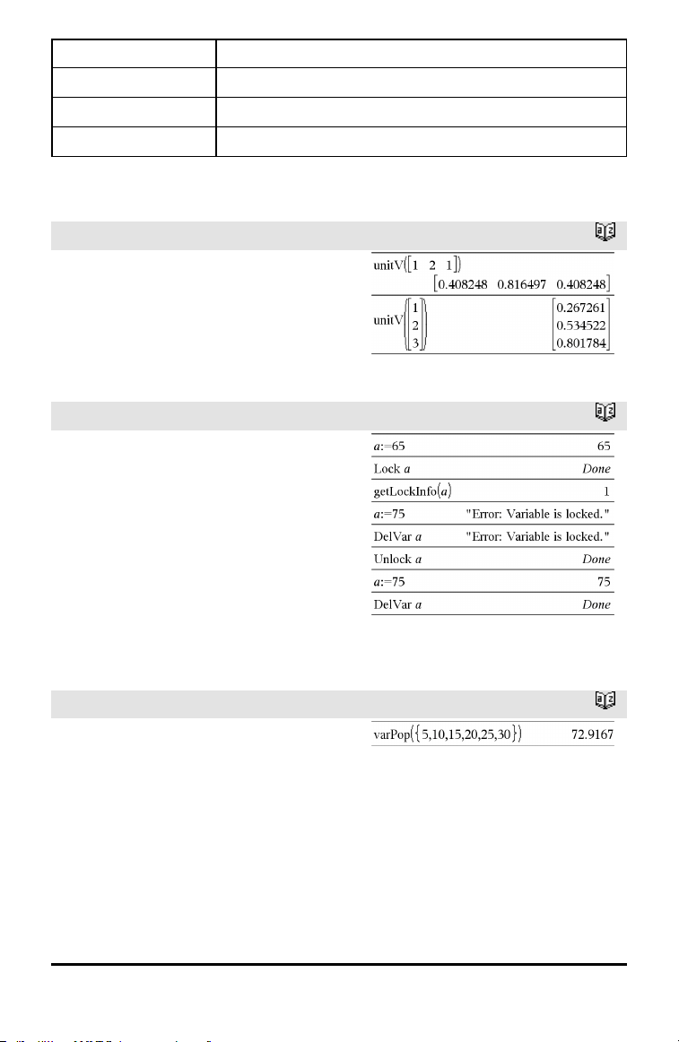
Output variable Description
stat.MaxY Maximum of y values
stat.Σ(x-v)
2
Sum of squares of deviations from the meanof x
stat.Σ(y-w)
2
Sum of squares of deviations from the meanof y
U
unitV()
Catalog >
unitV(Vector1) ⇒ vector
Returns either a row- or column-unit vector,
depending on the form of Vector1.
Vector1 must be either a single-row matrix
or a single-column matrix.
unLock
Catalog >
unLock Var1[, Var2] [, Var3] ...
unLock Var.
Unlocks the specified variables or variable
group. Locked variables cannot be modified
or deleted.
See Lock, page 85, and getLockInfo(), page
63.
V
varPop()
Catalog >
varPop(List[, freqList]) ⇒ expression
Returns the population variance of List.
Each freqList element counts the number
of consecutive occurrences of the
corresponding element in List.
Note: List must contain at least two
elements.
Alphabetical Listing 163
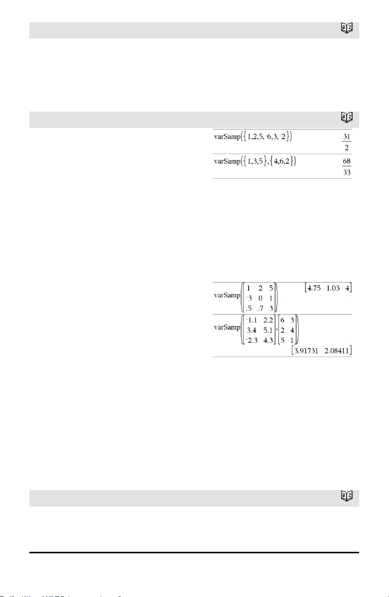
164 Alphabetical Listing
varPop()
Catalog >
If an element in either list is empty (void),
that element is ignored, and the
corresponding element in the other list is
also ignored. For more information on
empty elements, see page 196.
varSamp()
Catalog >
varSamp(List[, freqList]) ⇒ expression
Returns the sample variance of List.
Each freqList element counts the number
of consecutive occurrences of the
corresponding element in List.
Note: List must contain at least two
elements.
If an element in either list is empty (void),
that element is ignored, and the
corresponding element in the other list is
also ignored. For more information on
empty elements, see page 196.
varSamp(Matrix1[, freqMatrix]) ⇒
matrix
Returns a row vector containing the sample
variance of each column in Matrix1.
Each freqMatrix element counts the
number of consecutive occurrences of the
corresponding element in Matrix1.
If an element in either matrix is empty
(void), that element is ignored, and the
corresponding element in the other matrix
is also ignored. For more information on
empty elements, see page 196.
Note: Matrix1 must contain at least two
rows.
W
Wait
Catalog >
Wait timeInSeconds
To wait 4 seconds:
Wait 4
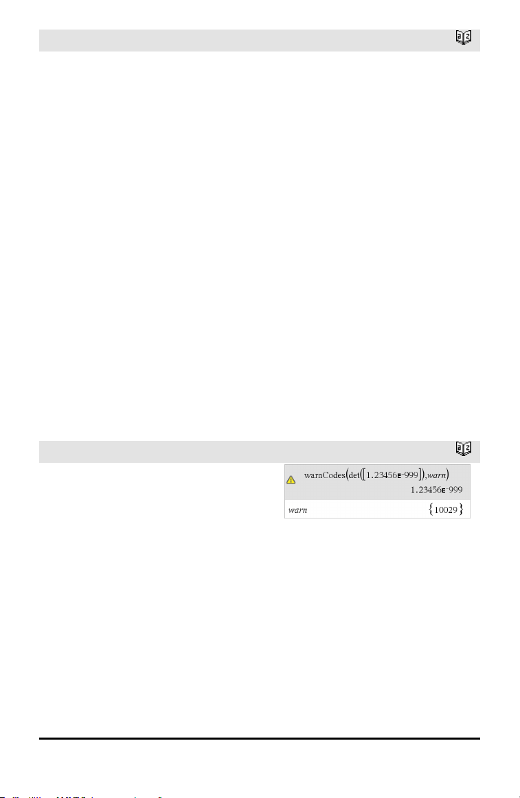
Wait
Catalog >
Suspends execution for a period of
timeInSeconds seconds.
Wait is particularly useful in a program that
needs a brief delay to allow requested data
to become available.
The argument timeInSeconds must be an
expression that simplifies to a decimal value
in the range 0 through 100. The command
rounds this value up to the nearest 0.1
seconds.
To cancel a Wait that is in progress,
• Handheld: Hold down the c key and
press · repeatedly.
• Windows®: Hold down the F12 key and
press Enter repeatedly.
• Macintosh®: Hold down the F5 key and
press Enter repeatedly.
• iPad®: The app displays a prompt. You can
continue waiting or cancel.
Note: You can use the Wait command within
a user-defined program but not within a
function.
To wait 1/2 second:
Wait 0.5
To wait 1.3 seconds using the variable
seccount:
seccount:=1.3
Wait seccount
This example switches a greenLED on for
0.5 seconds and then switches it off.
Send "SET GREEN 1 ON"
Wait 0.5
Send "SET GREEN 1 OFF"
warnCodes ()
Catalog >
warnCodes(Expr1, StatusVar) ⇒
expression
Evaluates expression Expr1, returns the
result, and stores the codes of any
generated warnings in the StatusVar list
variable. If no warnings are generated, this
function assigns StatusVar an empty list.
Expr1 can be any valid TI-Nspire™ or
TI-Nspire™CAS math expression. You
cannot use a command or assignment as
Expr1.
StatusVar must be a valid variable name.
For a list of warning codes and associated
messages, see page 211.
Alphabetical Listing 165
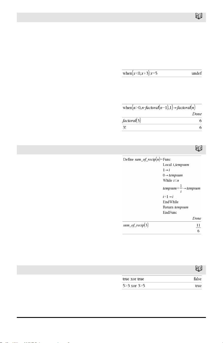
166 Alphabetical Listing
when()
Catalog >
when(Condition, trueResult [, falseResult]
[, unknownResult]) ⇒ expression
Returns trueResult, falseResult, or
unknownResult, depending on whether
Condition is true, false, or unknown.
Returns the input if there are too few
arguments to specify the appropriate result.
Omit both falseResult and unknownResult
to make an expression defined only in the
region where Condition is true.
Use an undef falseResult to define an
expression that graphs only on an interval.
when() is helpful for defining recursive
functions.
While
Catalog >
While Condition
Block
EndWhile
Executes the statements in Block as long
as Condition is true.
Block can be either a single statement or a
sequence of statements separated with the
“:” character.
Note for entering the example: For
instructions on entering multi-line program
and function definitions, refer to the
Calculator section of your product
guidebook.
X
xor
Catalog >
BooleanExpr1 xor BooleanExpr2 returns
Boolean expressionBooleanList1
xor BooleanList2 returns Boolean
listBooleanMatrix1
xor BooleanMatrix2 returns Boolean

xor
Catalog >
matrix
Returns true if BooleanExpr1 is true and
BooleanExpr2 is false, or vice versa.
Returns false if both arguments are true or
if both are false. Returns a simplified
Boolean expression if either of the
arguments cannot be resolved to true or
false.
Note: See or, page 107.
Integer1 xor Integer2⇒ integer
Compares two real integers bit-by-bit using
an xor operation. Internally, both integers
are converted to signed, 64-bit binary
numbers. When corresponding bits are
compared, the result is 1 if either bit (but
not both) is 1; the result is 0 if both bits are
0 or both bits are 1. The returned value
represents the bit results, and is displayed
according to the Base mode.
You can enter the integers in any number
base. For a binary or hexadecimal entry, you
must use the 0b or 0h prefix, respectively.
Without a prefix, integers are treated as
decimal (base10).
If you enter a decimal integer that is too
large for a signed, 64-bit binary form, a
symmetric modulo operation is used to
bring the value into the appropriate range.
For more information, see ►Base2, page
16.
Note: See or, page 107.
In Hex base mode:
Important: Zero, not the letter O.
In Bin base mode:
Note: A binary entry can have up to 64 digits
(not counting the 0b prefix). A hexadecimal
entry can have upto 16 digits.
Z
zInterval
Catalog >
zInterval σ,List[,Freq[,CLevel]]
(Data list input)
zInterval σ,v,n [,CLevel]
(Summary stats input)
Alphabetical Listing 167

168 Alphabetical Listing
zInterval
Catalog >
Computes a z confidence interval. A
summary of results is stored in the
stat.results variable. (See page 145.)
For information on the effect of empty
elements in a list, see “Empty (Void)
Elements,” page 196.
Output variable Description
stat.CLower, stat.CUpper Confidence interval for an unknown population mean
stat.x Sample mean of the data sequence from the normal random distribution
stat.ME Marginof error
stat.sx Sample standard deviation
stat.n Length of the data sequence with sample mean
stat.σ Knownpopulation standard deviation for data sequence List
zInterval_1Prop
Catalog >
zInterval_1Prop x,n [,CLevel]
Computes a one-proportion z confidence
interval. A summary of results is stored in
the stat.results variable. (See page 145.)
x is a non-negative integer.
For information on the effect of empty
elements in a list, see “Empty (Void)
Elements,” page 196.
Output variable Description
stat.CLower, stat.CUpper Confidence interval containing confidence levelprobability of distribution
stat.Ç The calculated proportion of successes
stat.ME Margin of error
stat.n Number of samples in data sequence
zInterval_2Prop
Catalog >
zInterval_2Prop x1,n1,x2,n2[,CLevel]

zInterval_2Prop
Catalog >
Computes a two-proportion z confidence
interval. A summary of results is stored in
the stat.results variable. (See page 145.)
x1 and x2 are non-negative integers.
For information on the effect of empty
elements in a list, see “Empty (Void)
Elements,” page 196.
Output variable Description
stat.CLower, stat.CUpper Confidence interval containing confidence levelprobability of distribution
stat.Ç Diff The calculated difference betweenproportions
stat.ME Margin of error
stat.Ç1 First sample proportion estimate
stat.Ç2 Second sample proportion estimate
stat.n1 Sample size in data sequence one
stat.n2 Sample size in data sequence two
zInterval_2Samp
Catalog >
zInterval_2Samp σ
1
,σ
2
,List1,List2[,Freq1
[,Freq2,[CLevel]]]
(Data list input)
zInterval_2Samp σ
1
,σ
2
,v1,n1,v2,n2
[,CLevel]
(Summary stats input)
Computes a two-sample z confidence
interval. A summary of results is stored in
the stat.results variable. (See page 145.)
For information on the effect of empty
elements in a list, see “Empty (Void)
Elements,” page 196.
Output variable Description
stat.CLower,
stat.CUpper
Confidence interval containing confidence levelprobability of distribution
Alphabetical Listing 169

170 Alphabetical Listing
Output variable Description
stat.x1-x2 Sample means of the data sequences from the normal random
distribution
stat.ME Margin of error
stat.x1, stat.x2 Sample means of the data sequences from the normal random
distribution
stat.σx1, stat.σx2 Sample standard deviations for List 1 and List 2
stat.n1, stat.n2 Number of samples indata sequences
stat.r1, stat.r2
Knownpopulation standard deviations for data sequence List 1 andList
2
zTest
Catalog >
zTest μ0,σ,List,[Freq[,Hypoth]]
(Data list input)
zTest μ0,σ,v,n[,Hypoth]
(Summary stats input)
Performs a z test with frequency freqlist. A
summary of results is stored in the
stat.results variable. (See page 145.)
Test H
0
: μ = μ0, against one of the
following:
For H
a
: μ < μ0, set Hypoth<0
For H
a
: μ ≠ μ0 (default), set Hypoth=0
For H
a
: μ > μ0, set Hypoth>0
For information on the effect of empty
elements in a list, see “Empty (Void)
Elements,” page 196.
Output variable Description
stat.z
(x − μ0) / (σ / sqrt(n))
stat.P Value Least probability at which the null hypothesis can be rejected
stat.x
Sample mean of the data sequence inList
stat.sx
Sample standard deviation of the data sequence. Only returned for Data input.
stat.n Size of the sample

zTest_1Prop
Catalog >
Output variable Description
stat.p0 Hypothesized population proportion
stat.z Standard normal value computedfor the proportion
stat.PVal Smallest level of significance at whichthe null hypothesis can be rejected
stat.Ç Estimated sample proportion
stat.n Size of the sample
zTest_2Prop
Catalog >
zTest_2Prop x1,n1,x2,n2[,Hypoth]
Computes a two-proportion z test. A
summary of results is stored in the
stat.results variable. (See page 145.)
x1 and x2 are non-negative integers.
Test H
0
: p1 = p2, against one of the
following:
For H
a
: p1 > p2, set Hypoth>0
For H
a
: p1 ≠ p2 (default), set Hypoth=0
For H
a
: p < p0, set Hypoth<0
For information on the effect of empty
elements in a list, see “Empty (Void)
Elements,” page 196.
Output variable Description
stat.z Standard normal value computedfor the difference of proportions
stat.PVal Smallest level of significance at whichthe null hypothesis can be rejected
stat.Ç1 First sample proportion estimate
stat.Ç2 Second sample proportion estimate
stat.Ç Pooled sample proportion estimate
stat.n1, stat.n2 Number of samples takenin trials 1 and2
zTest_2Samp
Catalog >
zTest_2Samp σ
1
,σ
2
,List1,List2[,Freq1
Alphabetical Listing 171

172 Alphabetical Listing
zTest_2Samp
Catalog >
[,Freq2[,Hypoth]]]
(Data list input)
zTest_2Samp σ
1
,σ
2
,v1,n1,v2,n2[,Hypoth]
(Summary stats input)
Computes a two-sample z test. A summary
of results is stored in the stat.results
variable. (See page 145.)
Test H
0
: μ1 = μ2, against one of the
following:
For H
a
: μ1 < μ2, set Hypoth<0
For H
a
: μ1 ≠ μ2 (default), set Hypoth=0
For H
a
: μ1 > μ2, Hypoth>0
For information on the effect of empty
elements in a list, see “Empty (Void)
Elements,” page 196.
Output variable Description
stat.z Standard normal value computedfor the difference of means
stat.PVal Smallest level of significance at whichthe null hypothesis can be rejected
stat.x1, stat.x2
Sample means of the data sequences in List1 andList2
stat.sx1, stat.sx2
Sample standard deviations of the data sequences inList1 and List2
stat.n1, stat.n2 Size of the samples
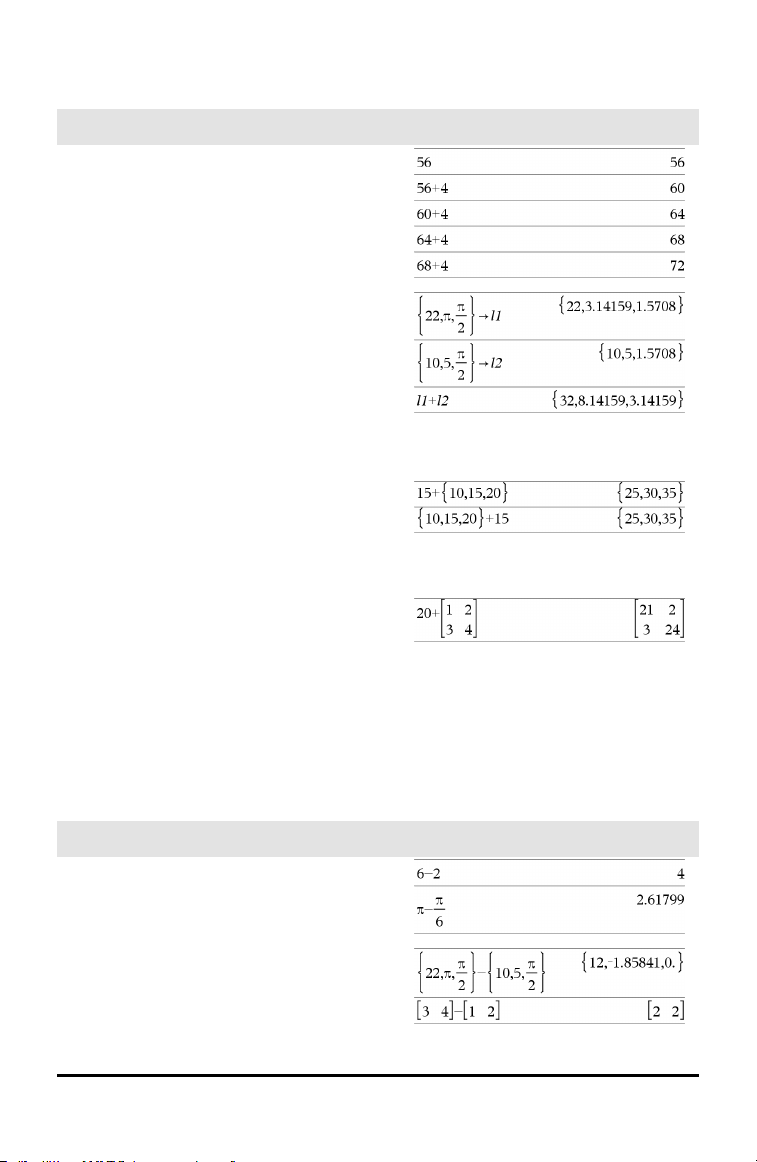
Symbols
+ (add)
+ key
Value1 + Value2 ⇒ value
Returns the sum of the two arguments.
List1 + List2 ⇒ list
Matrix1 + Matrix2 ⇒ matrix
Returns a list (or matrix) containing the
sums of corresponding elements in List1
and List2 (or Matrix1 and Matrix2).
Dimensions of the arguments must be
equal.
Value + List1 ⇒ list
List1 + Value ⇒ list
Returns a list containing the sums of Value
and each element in List1.
Value + Matrix1 ⇒ matrix
Matrix1 + Value ⇒ matrix
Returns a matrix with Value added to each
element on the diagonal of Matrix1.
Matrix1 must be square.
Note: Use .+ (dot plus) to add an expression
to each element.
− (subtract)
- key
Value1−Value2 ⇒ value
Returns Value1 minus Value2.
List1 −List2⇒ list
Matrix1 −Matrix2 ⇒ matrix
Symbols 173
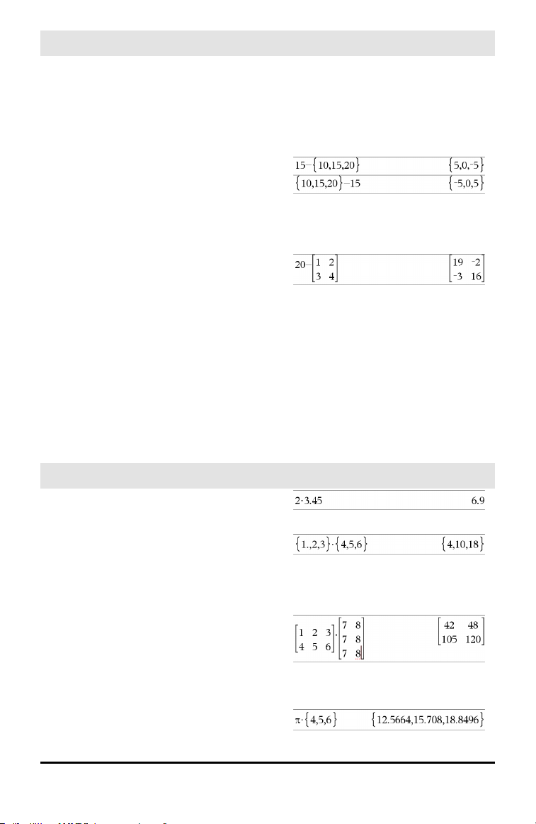
174 Symbols
− (subtract)
- key
Subtracts each element in List2 (or
Matrix2) from the corresponding element
in List1 (or Matrix1), and returns the
results.
Dimensions of the arguments must be
equal.
Value − List1 ⇒ list
List1 − Value ⇒ list
Subtracts each List1 element from Value
or subtracts Value from each List1
element, and returns a list of the results.
Value − Matrix1 ⇒ matrix
Matrix1 − Value ⇒ matrix
Value − Matrix1 returns a matrix of Value
times the identity matrix minus
Matrix1.Matrix1 must be square.
Matrix1 − Value returns a matrix of Value
times the identity matrix subtracted from
Matrix1.Matrix1 must be square.
Note: Use .− (dot minus) to subtract an
expression from each element.
• (multiply)
r key
Value1•Value2 ⇒ value
Returns the product of the two arguments.
List1•List2 ⇒ list
Returns a list containing the products of the
corresponding elements in List1 and List2.
Dimensions of the lists must be equal.
Matrix1•Matrix2 ⇒ matrix
Returns the matrix product of Matrix1 and
Matrix2.
The number of columns in Matrix1 must
equal the number of rows in Matrix2.
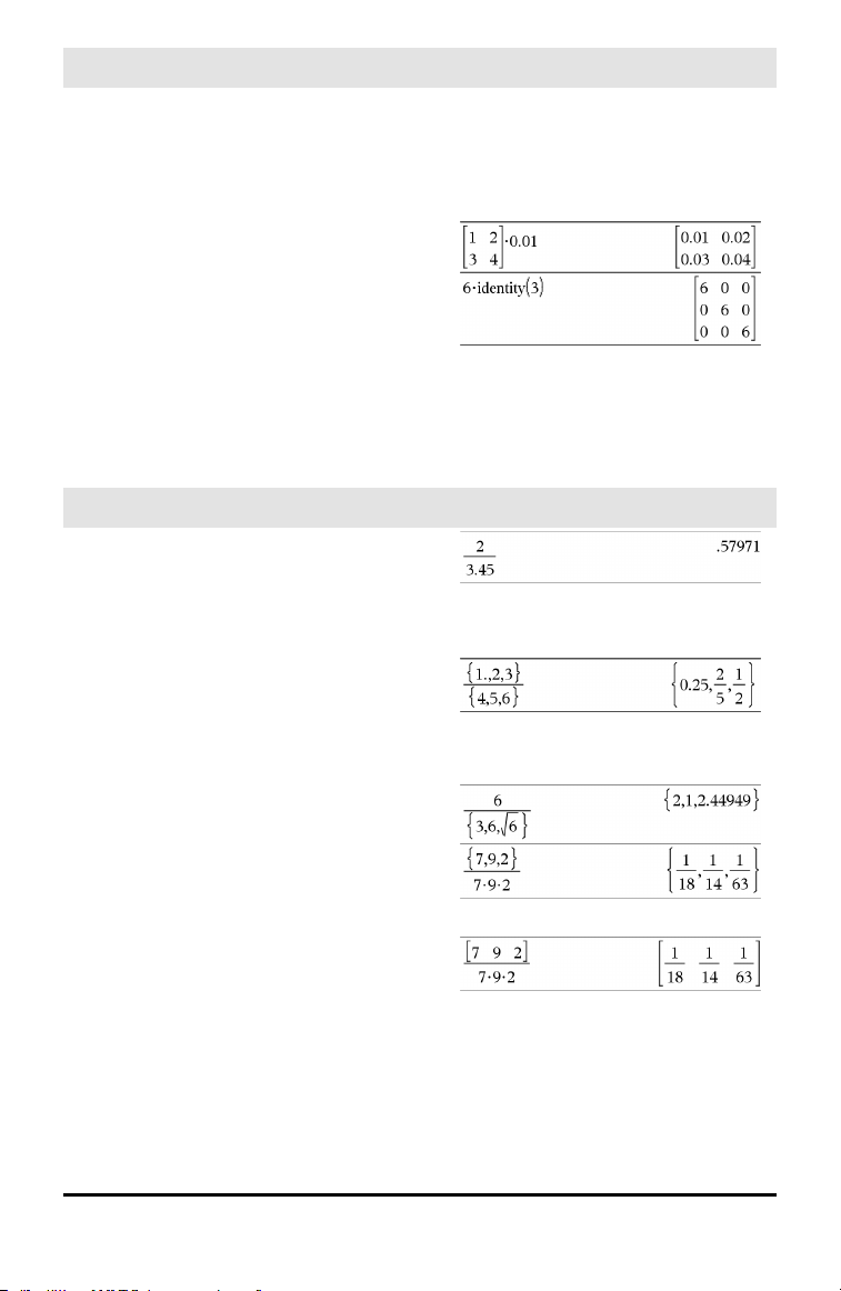
• (multiply)
r key
Value •List1 ⇒ list
List1•Value ⇒ list
Returns a list containing the products of
Value and each element in List1.
Value •Matrix1 ⇒ matrix
Matrix1•Value ⇒ matrix
Returns a matrix containing the products of
Value and each element in Matrix1.
Note: Use .•(dot multiply) to multiply an
expression by each element.
⁄ (divide)
p key
Value1 ⁄ Value2 ⇒ value
Returns the quotient of Value1 divided by
Value2.
Note: See also Fraction template, page 1.
List1 ⁄ List2 ⇒ list
Returns a list containing the quotients of
List1 divided by List2.
Dimensions of the lists must be equal.
Value ⁄ List1 ⇒ list
List1 ⁄ Value ⇒ list
Returns a list containing the quotients of
Value divided by List1 or List1 divided by
Value.
Value ⁄ Matrix1 ⇒ matrix
Matrix1 ⁄ Value ⇒ matrix
Returns a matrix containing the quotients
of Matrix1 ⁄ Value.
Note: Use . ⁄ (dot divide) to divide an
expression by each element.
Symbols 175
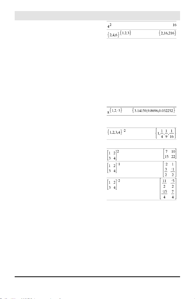
176 Symbols
^ (power)
l key
Value1 ^ Value2⇒ value
List1 ^ List2 ⇒ list
Returns the first argument raised to the
power of the second argument.
Note: See also Exponent template, page 1.
For a list, returns the elements in List1
raised to the power of the corresponding
elements in List2.
In the real domain, fractional powers that
have reduced exponents with odd
denominators use the real branch versus
the principal branch for complex mode.
Value ^ List1 ⇒ list
Returns Value raised to the power of the
elements in List1.
List1 ^ Value ⇒ list
Returns the elements in List1 raised to the
power of Value.
squareMatrix1 ^ integer ⇒ matrix
Returns squareMatrix1 raised to the
integer power.
squareMatrix1 must be a square matrix.
If integer = −1, computes the inverse
matrix.
If integer < −1, computes the inverse
matrix to an appropriate positive power.
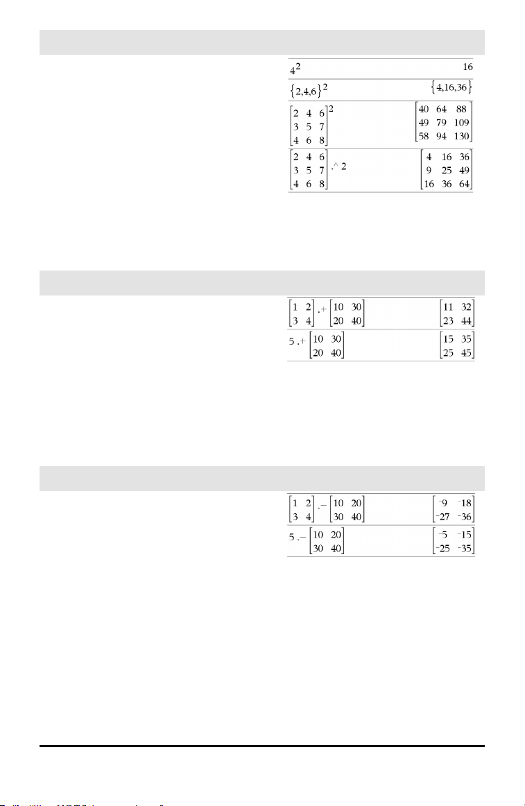
x
2
(square)
q key
Value1
2
⇒ value
Returns the square of the argument.
List1
2
⇒ list
Returns a list containing the squares of the
elements in List1.
squareMatrix1
2
⇒ matrix
Returns the matrix square of
squareMatrix1. This is not the same as
calculating the square of each element. Use
.^2 to calculate the square of each element.
.+ (dot add)
^+ keys
Matrix1 .+ Matrix2 ⇒ matrix
Value .+ Matrix1⇒ matrix
Matrix1.+Matrix2 returns a matrix that is
the sum of each pair of corresponding
elements in Matrix1 and Matrix2.
Value .+ Matrix1 returns a matrix that is
the sum of Value and each element in
Matrix1.
.⁻(dot subt.)
^- keys
Matrix1 .− Matrix2⇒ matrix
Value .− Matrix1 ⇒ matrix
Matrix1.− Matrix2 returns a matrix that is
the difference between each pair of
corresponding elements in Matrix1 and
Matrix2.
Value .− Matrix1 returns a matrix that is
the difference of Value and each element
in Matrix1.
Symbols 177
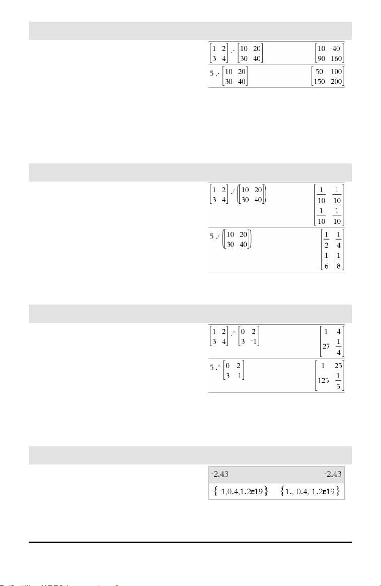
178 Symbols
.•(dot mult.)
^r keys
Matrix1 .• Matrix2⇒ matrix
Value .• Matrix1 ⇒ matrix
Matrix1.• Matrix2 returns a matrix that is
the product of each pair of corresponding
elements in Matrix1 and Matrix2.
Value .• Matrix1 returns a matrix
containing the products of Value and each
element in Matrix1.
. ⁄ (dot divide)
^p keys
Matrix1. ⁄ Matrix2 ⇒ matrix
Value . ⁄ Matrix1⇒ matrix
Matrix1 . ⁄ Matrix2 returns a matrix that is
the quotient of each pair of corresponding
elements in Matrix1 and Matrix2.
Value . ⁄ Matrix1 returns a matrix that is
the quotient of Value and each element in
Matrix1.
.^ (dot power)
^l keys
Matrix1 .^ Matrix2 ⇒ matrix
Value . ^ Matrix1⇒ matrix
Matrix1.^ Matrix2 returns a matrix where
each element in Matrix2 is the exponent
for the corresponding element in Matrix1.
Value .^ Matrix1 returns a matrix where
each element in Matrix1 is the exponent
for Value.
− (negate)
v key
−Value1 ⇒ value
−List1 ⇒ list
−Matrix1 ⇒ matrix

− (negate)
v key
Returns the negation of the argument.
For a list or matrix, returns all the elements
negated.
If the argument is a binary or hexadecimal
integer, the negation gives the two’s
complement.
In Bin base mode:
Important: Zero, not the letter O.
To see the entire result, press £ and then
use ¡and¢ to move the cursor.
% (percent)
/k keys
Value1% ⇒ value
List1% ⇒ list
Matrix1% ⇒ matrix
Returns
For a list or matrix, returns a list or matrix
with each element divided by 100.
= (equal)
= key
Expr1=Expr2 ⇒ Boolean expression
List1=List2 ⇒ Boolean list
Matrix1=Matrix2 ⇒ Boolean matrix
Returns true if Expr1 is determined to be
equal to Expr2.
Returns false if Expr1 is determined to not
be equal to Expr2.
Anything else returns a simplified form of
the equation.
For lists and matrices, returns comparisons
element by element.
Example function that uses math test
symbols: =, ≠, <, ≤, >, ≥
Resultof graphing g(x)
Symbols 179
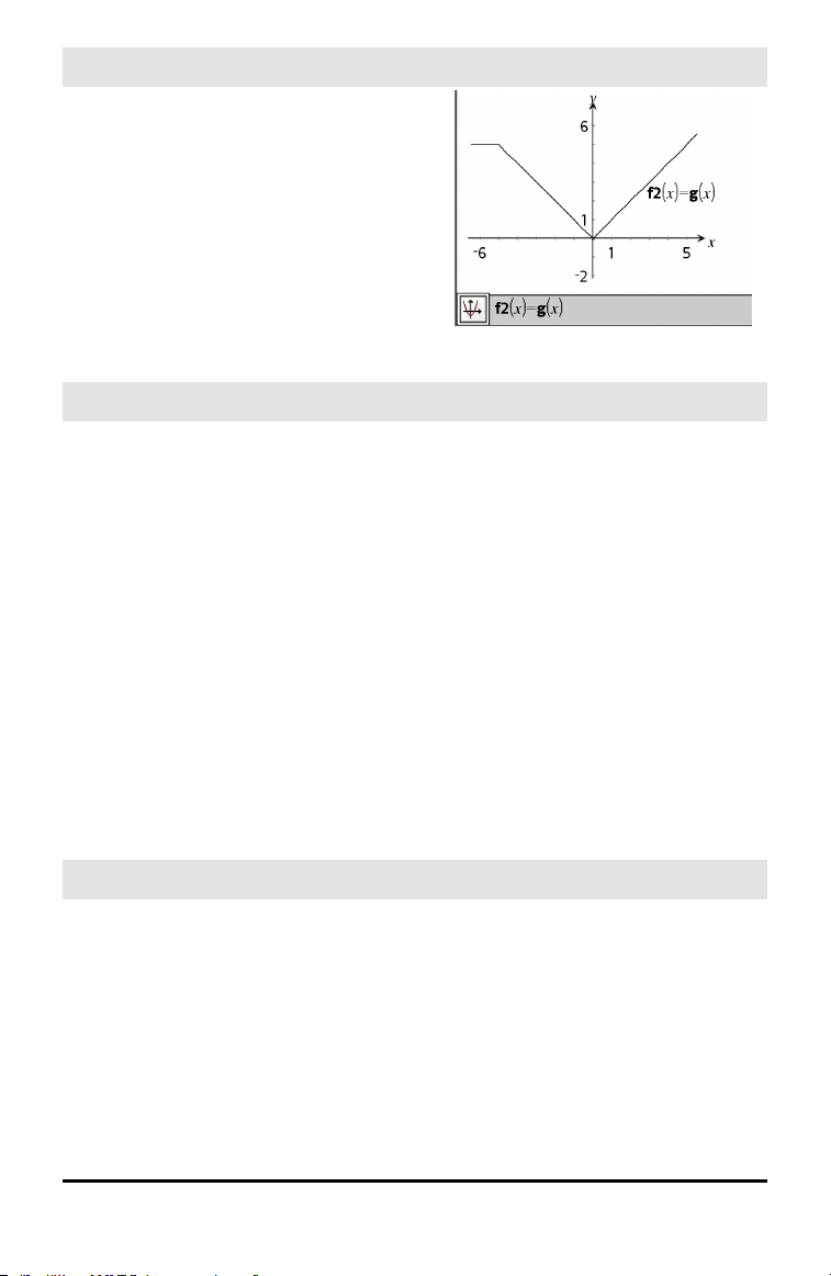
180 Symbols
= (equal)
= key
Note for entering the example: For
instructions on entering multi-line program
and function definitions, refer to the
Calculator section of your product
guidebook.
≠ (not equal)
/= keys
Expr1≠Expr2 ⇒ Boolean expression
List1≠List2 ⇒ Boolean list
Matrix1≠Matrix2 ⇒ Boolean matrix
Returns true if Expr1 is determined to be
not equal to Expr2.
Returns false if Expr1 is determined to be
equal to Expr2.
Anything else returns a simplified form of
the equation.
For lists and matrices, returns comparisons
element by element.
Note: You can insert this operator from the
keyboard by typing /=
See “=” (equal) example.
< (less than)
/= keys
Expr1<Expr2 ⇒ Boolean expression
List1<List2 ⇒ Boolean list
Matrix1<Matrix2 ⇒ Boolean matrix
Returns true if Expr1 is determined to be
less than Expr2.
Returns false if Expr1 is determined to be
greater than or equal to Expr2.
See “=” (equal) example.

< (less than)
/= keys
Anything else returns a simplified form of
the equation.
For lists and matrices, returns comparisons
element by element.
≤ (less or equal)
/= keys
Expr1≤Expr2 ⇒ Boolean expression
List1≤List2 ⇒ Boolean list
Matrix1 ≤Matrix2 ⇒ Boolean matrix
Returns true if Expr1 is determined to be
less than or equal to Expr2.
Returns false if Expr1 is determined to be
greater than Expr2.
Anything else returns a simplified form of
the equation.
For lists and matrices, returns comparisons
element by element.
Note: You can insert this operator from the
keyboard by typing <=
See “=” (equal) example.
> (greater than)
/= keys
Expr1>Expr2 ⇒ Boolean expression
List1>List2 ⇒ Boolean list
Matrix1>Matrix2 ⇒ Boolean matrix
Returns true if Expr1 is determined to be
greater than Expr2.
Returns false if Expr1 is determined to be
less than or equal to Expr2.
Anything else returns a simplified form of
the equation.
For lists and matrices, returns comparisons
element by element.
See “=” (equal) example.
Symbols 181
182 Symbols
≥ (greater or equal)
/= keys
Expr1≥Expr2 ⇒ Boolean expression
List1≥List2 ⇒ Boolean list
Matrix1 ≥Matrix2 ⇒ Boolean matrix
Returns true if Expr1 is determined to be
greater than or equal to Expr2.
Returns false if Expr1 is determined to be
less than Expr2.
Anything else returns a simplified form of
the equation.
For lists and matrices, returns comparisons
element by element.
Note: You can insert this operator from the
keyboard by typing >=
See “=” (equal) example.
⇒ (logical implication)
/= keys
BooleanExpr1 ⇒ BooleanExpr2 returns
Boolean expression
BooleanList1 ⇒ BooleanList2 returns
Boolean list
BooleanMatrix1 ⇒ BooleanMatrix2
returns Boolean matrix
Integer1 ⇒ Integer2 returns Integer
Evaluates the expression not <argument1>
or <argument2> and returns true, false, or a
simplified form of the equation.
For lists and matrices, returns comparisons
element by element.
Note: You can insert this operator from the
keyboard by typing =>
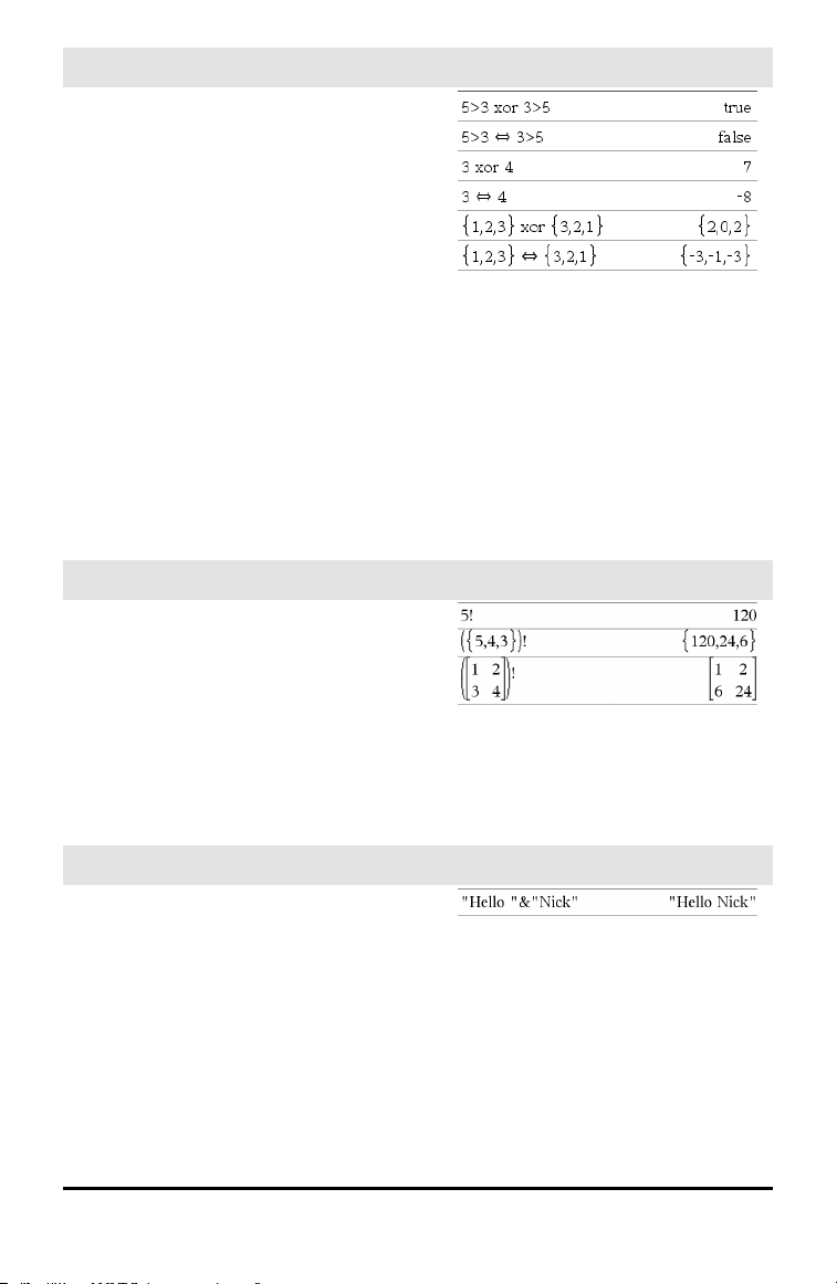
⇔ (logical double implication, XNOR)
/= keys
BooleanExpr1 ⇔ BooleanExpr2 returns
Boolean expression
BooleanList1 ⇔ BooleanList2 returns
Boolean list
BooleanMatrix1 ⇔ BooleanMatrix2
returns Boolean matrix
Integer1 ⇔ Integer2 returns Integer
Returns the negation of an XOR Boolean
operation on the two arguments. Returns
true, false, or a simplified form of the
equation.
For lists and matrices, returns comparisons
element by element.
Note: You can insert this operator from the
keyboard by typing <=>
! (factorial)
º key
Value1! ⇒ value
List1! ⇒ list
Matrix1! ⇒ matrix
Returns the factorial of the argument.
For a list or matrix, returns a list or matrix
of factorials of the elements.
& (append)
/k keys
String1 & String2 ⇒ string
Returns a text string that is String2
appended to String1.
Symbols 183
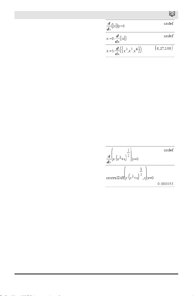
184 Symbols
d() (derivative)
Catalog >
d(Expr1, Var[, Order]) | Var=Value ⇒
value
d(Expr1, Var[, Order]) ⇒ value
d(List1, Var[, Order]) ⇒ list
d(Matrix1, Var[, Order]) ⇒ matrix
Except when using the first syntax, you
must store a numeric value in variable Var
before evaluating d(). Refer to the
examples.
d() can be used for calculating first and
second order derivative at a point
numerically, using auto differentiation
methods.
Order, if included, must be=1 or 2. The
default is 1.
Note: You can insert this function from the
keyboard by typing derivative(...).
Note: See also Firstderivative, page 5 or
Secondderivative, page 5.
Note: The d() algorithm has a limitation: it
works recursively through the unsimplified
expression, computing the numeric value of
the first derivative (and second, if
applicable) and the evaluation of each
subexpression, which may lead to an
unexpected result.
Consider the example on the right. The first
derivative of x•(x^2+x)^(1/3) at x=0 is equal
to 0. However, because the first derivative
of the subexpression (x^2+x)^(1/3) is
undefined at x=0, and this value is used to
calculate the derivative of the total
expression, d() reports the result as
undefined and displays a warning message.
If you encounter this limitation, verify the
solution graphically. You can also try using
centralDiff().
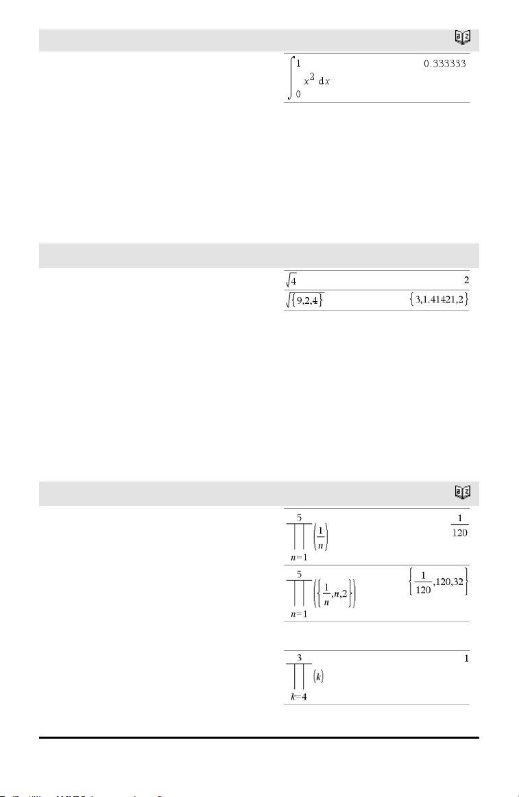
∫() (integral)
Catalog >
∫(Expr1, Var, Lower,Upper) ⇒ value
Returns the integral of Expr1 with respect
to the variable Var from Lower to Upper.
Can be used to calculate the definite
integral numerically, using the same
method as nInt().
Note: You can insert this function from the
keyboard by typing integral(...).
Note: See also nInt(), page 101, and
Definiteintegral template, page 6.
√() (square root)
/q keys
√(Value1) ⇒ value
√(List1) ⇒ list
Returns the square root of the argument.
For a list, returns the square roots of all the
elements in List1.
Note: You can insert this function from the
keyboard by typing sqrt(...)
Note: See also Square root template, page
1.
Π() (prodSeq)
Catalog >
Π(Expr1, Var, Low, High) ⇒ expression
Note: You can insert this function from the
keyboard by typing prodSeq(...).
Evaluates Expr1 for each value of Var from
Low to High, and returns the product of the
results.
Note: See also Product template (Π), page
5.
Π(Expr1, Var, Low, Low−1) ⇒ 1
Π(Expr1, Var, Low, High) ⇒ 1/Π(Expr1,
Var, High+1, Low−1) if High < Low−1
Symbols 185
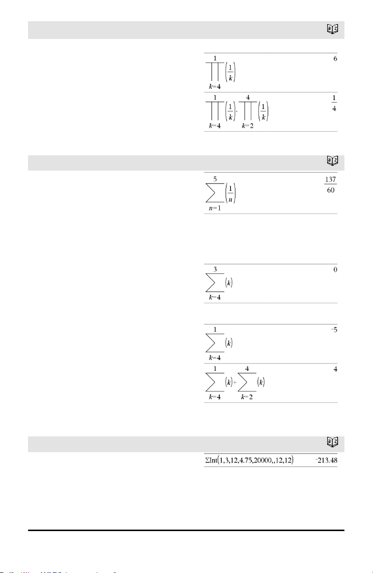
186 Symbols
Π() (prodSeq)
Catalog >
The product formulas used are derived from
the following reference:
Ronald L. Graham, Donald E. Knuth, and
Oren Patashnik. Concrete Mathematics: A
Foundation for Computer Science.
Reading, Massachusetts: Addison-Wesley,
1994.
Σ() (sumSeq)
Catalog >
Σ(Expr1, Var, Low, High) ⇒ expression
Note: You can insert this function from the
keyboard by typing sumSeq(...).
Evaluates Expr1 for each value of Var from
Low to High, and returns the sum of the
results.
Note: See also Sum template, page 5.
Σ(Expr1, Var, Low, Low−1) ⇒ 0
Σ(Expr1, Var, Low, High) ⇒ μ
Σ(Expr1, Var, High+1, Low−1) if High <
Low−1
The summation formulas used are derived
from the following reference:
Ronald L. Graham, Donald E. Knuth, and
Oren Patashnik. Concrete Mathematics: A
Foundation for Computer Science.
Reading, Massachusetts: Addison-Wesley,
1994.
ΣInt()
Catalog >
ΣInt(NPmt1, NPmt2, N, I, PV ,[Pmt], [FV],
[PpY], [CpY], [PmtAt], [roundValue])
⇒ value
ΣInt(NPmt1,NPmt2,amortTable) ⇒ value
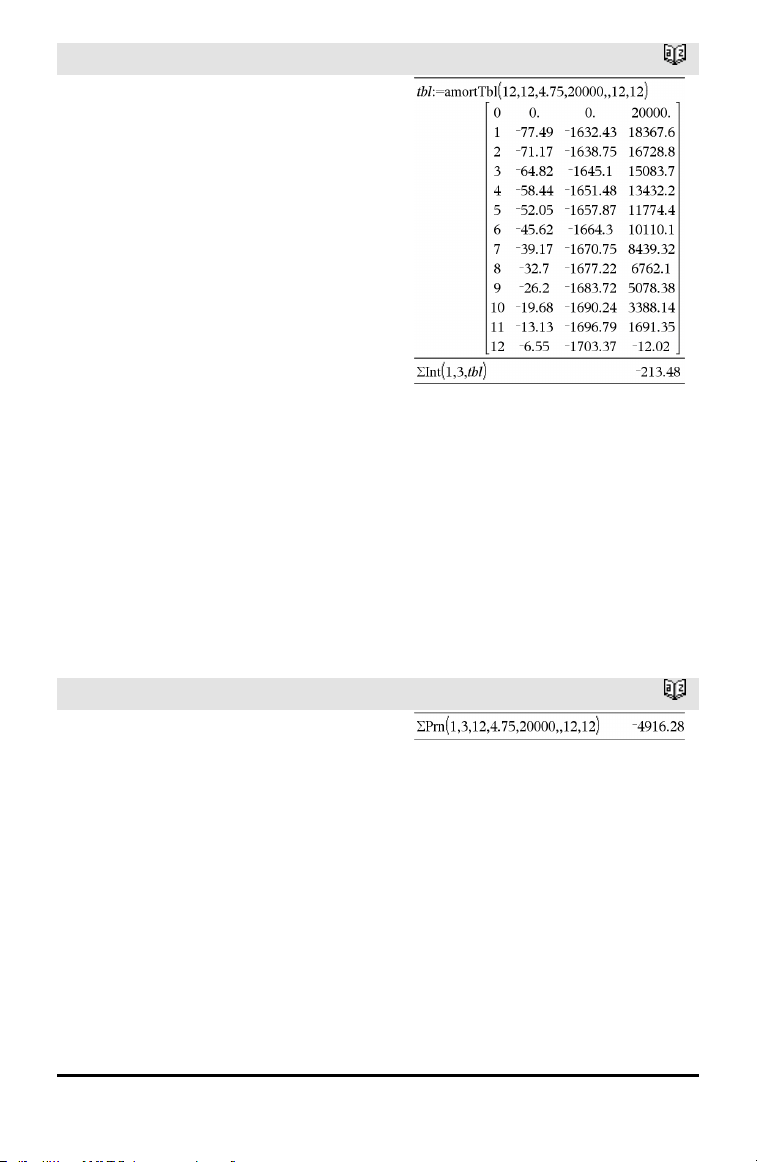
ΣInt()
Catalog >
Amortization function that calculates the
sum of the interest during a specified range
of payments.
NPmt1 and NPmt2 define the start and end
boundaries of the payment range.
N, I, PV, Pmt, FV, PpY, CpY, and PmtAt
are described in the table of TVM
arguments, page 161.
• If you omit Pmt, it defaults to
Pmt=tvmPmt
(N,I,PV,FV,PpY,CpY,PmtAt).
• If you omit FV, it defaults to FV=0.
• The defaults for PpY, CpY, and PmtAt
are the same as for the TVM functions.
roundValue specifies the number of
decimal places for rounding. Default=2.
ΣInt(NPmt1,NPmt2,amortTable) calculates
the sum of the interest based on
amortization table amortTable. The
amortTable argument must be a matrix in
the form described under amortTbl(), page
7.
Note: See also ΣPrn(), below, and Bal(),
page 15.
ΣPrn()
Catalog >
ΣPrn(NPmt1, NPmt2, N, I, PV, [Pmt],
[FV], [PpY], [CpY], [PmtAt],
[roundValue]) ⇒ value
ΣPrn(NPmt1, NPmt2, amortTable) ⇒
value
Amortization function that calculates the
sum of the principal during a specified
range of payments.
NPmt1 and NPmt2 define the start and end
boundaries of the payment range.
N, I, PV, Pmt, FV, PpY, CpY, and PmtAt
are described in the table of TVM
arguments, page 161.
Symbols 187
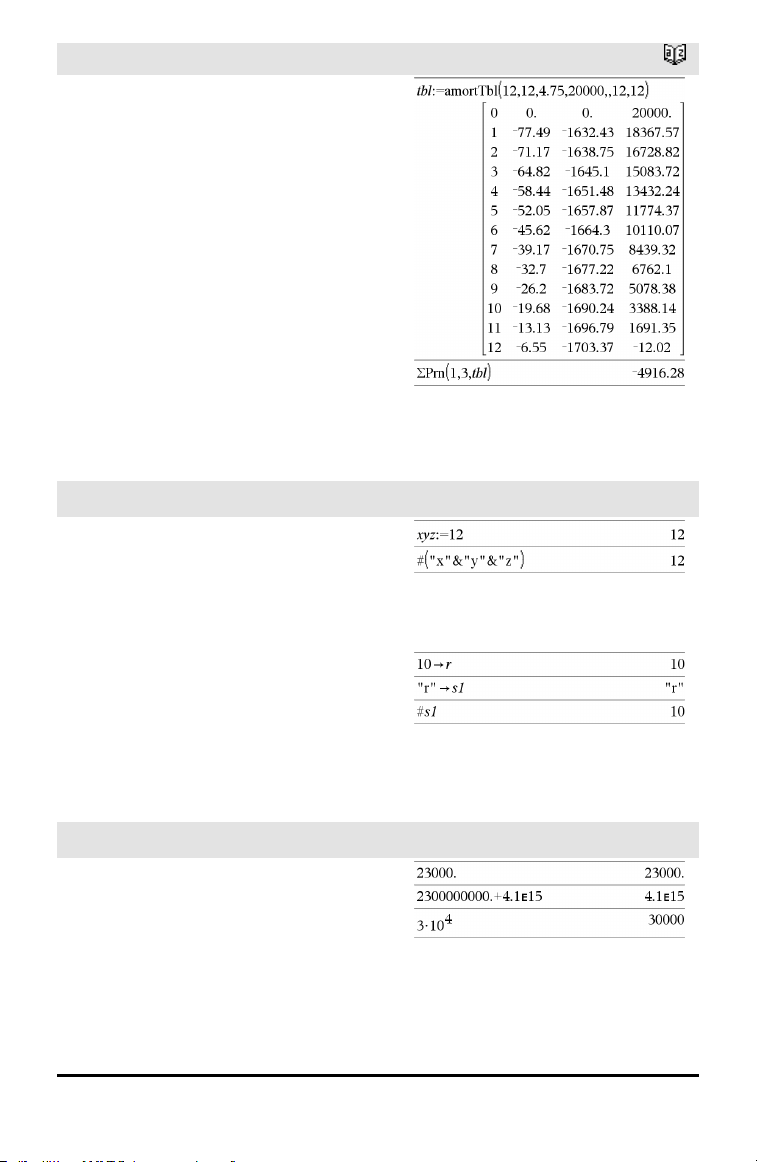
188 Symbols
ΣPrn()
Catalog >
• If you omit Pmt, it defaults to
Pmt=tvmPmt
(N,I,PV,FV,PpY,CpY,PmtAt).
• If you omit FV, it defaults to FV=0.
• The defaults for PpY, CpY, and PmtAt
are the same as for the TVM functions.
roundValue specifies the number of
decimal places for rounding. Default=2.
ΣPrn(NPmt1,NPmt2,amortTable)
calculates the sum of the principal paid
based on amortization table amortTable.
The amortTable argument must be a
matrix in the form described under
amortTbl(), page 7.
Note: See also ΣInt(), above, and Bal(),
page 15.
# (indirection)
/k keys
# varNameString
Refers to the variable whose name is
varNameString. This lets you use strings to
create variable names from within a
function.
Creates or refers to the variable xyz .
Returns the value of the variable (r) whose
name is stored in variable s1.
E (scientific notation)
i key
mantissaEexponent
Enters a number in scientific notation. The
number is interpreted as
mantissa ×10
exponent
.
Hint: If you want to enter a power of 10
without causing a decimal value result, use
10^integer.
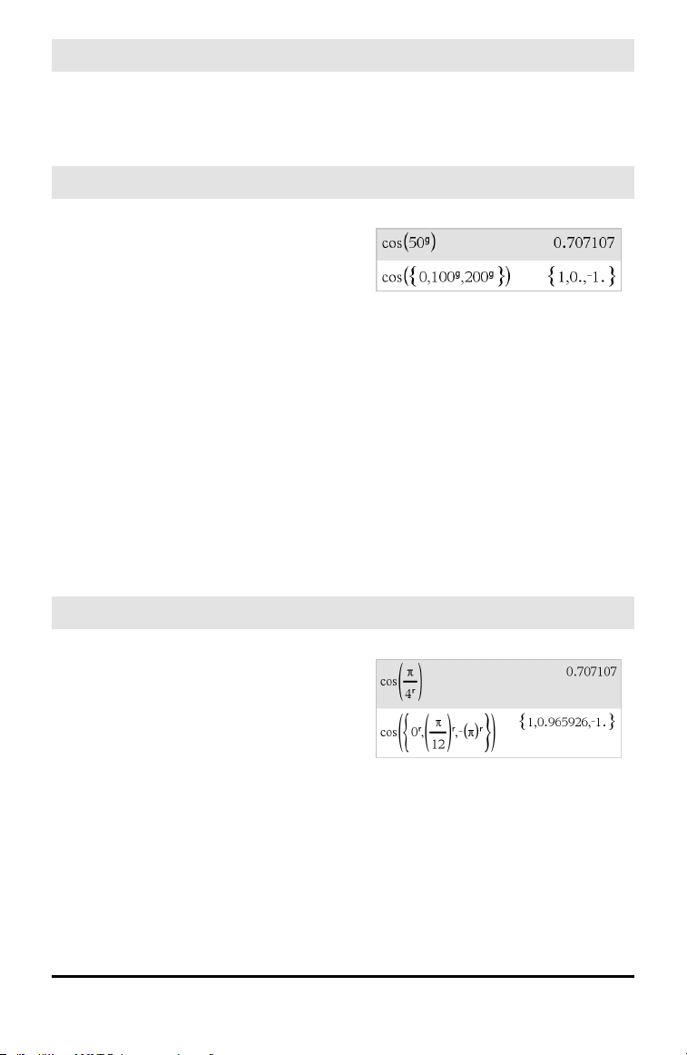
E (scientific notation)
i key
Note: You can insert this operator from the
computer keyboard by typing @E. for
example, type 2.3@E4 to enter 2.3E4.
g
(gradian)
¹ key
Expr1
g
⇒ expression
List1
g
⇒ list
Matrix1
g
⇒ matrix
This function gives you a way to specify a
gradian angle while in the Degree or Radian
mode.
In Radian angle mode, multiplies Expr1 by
π/200.
In Degree angle mode, multiplies Expr1 by
g/100.
In Gradian mode, returns Expr1 unchanged.
Note: You can insert this symbol from the
computer keyboard by typing @g.
In Degree, Gradian or Radian mode:
r
(radian)
¹ key
Value1
r
⇒ value
List1
r
⇒ list
Matrix1
r
⇒ matrix
This function gives you a way to specify a
radian angle while in Degree or Gradian
mode.
In Degree angle mode, multiplies the
argument by 180/π.
In Radian angle mode, returns the
argument unchanged.
In Gradian mode, multiplies the argument
by 200/π.
In Degree, Gradian or Radian angle mode:
Symbols 189
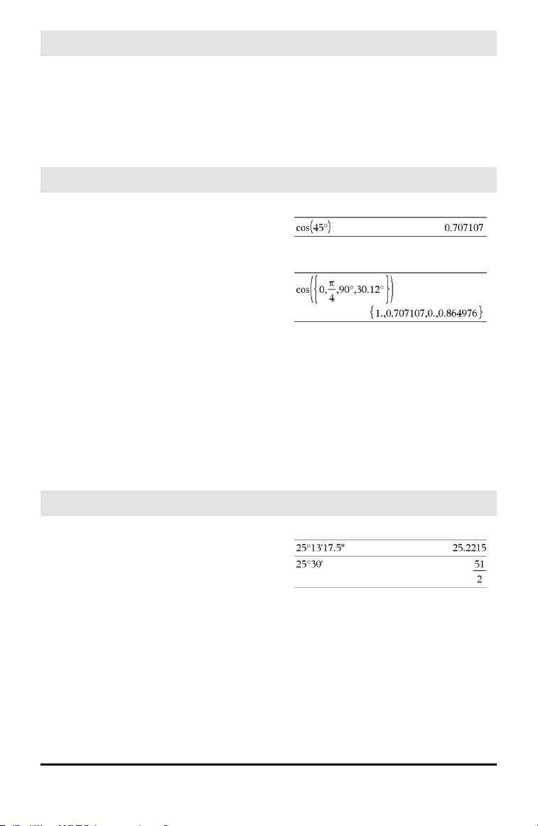
190 Symbols
r
(radian)
¹ key
Hint: Use
r
if you want to force radians in a
function definition regardless of the mode
that prevails when the function is used.
Note: You can insert this symbol from the
computer keyboard by typing @r.
° (degree)
¹ key
Value1° ⇒ value
List1° ⇒ list
Matrix1° ⇒ matrix
This function gives you a way to specify a
degree angle while in Gradian or Radian
mode.
In Radian angle mode, multiplies the
argument by π/180.
In Degree angle mode, returns the
argument unchanged.
In Gradian angle mode, multiplies the
argument by 10/9.
Note: You can insert this symbol from the
computer keyboard by typing @d.
In Degree, Gradian or Radian angle mode:
In Radian angle mode:
°, ', '' (degree/minute/second)
/k keys
dd°mm'ss.ss'' ⇒ expression
dd A positive or negative number
mm A non-negative number
ss.ss A non-negative number
Returns dd+(mm/60)+(ss.ss/3600).
This base-60 entry format lets you:
• Enter an angle in
degrees/minutes/seconds without regard
to the current angle mode.
• Enter time as hours/minutes/seconds.
Note: Follow ss.ss with two apostrophes
(''), not a quote symbol (").
In Degree angle mode:
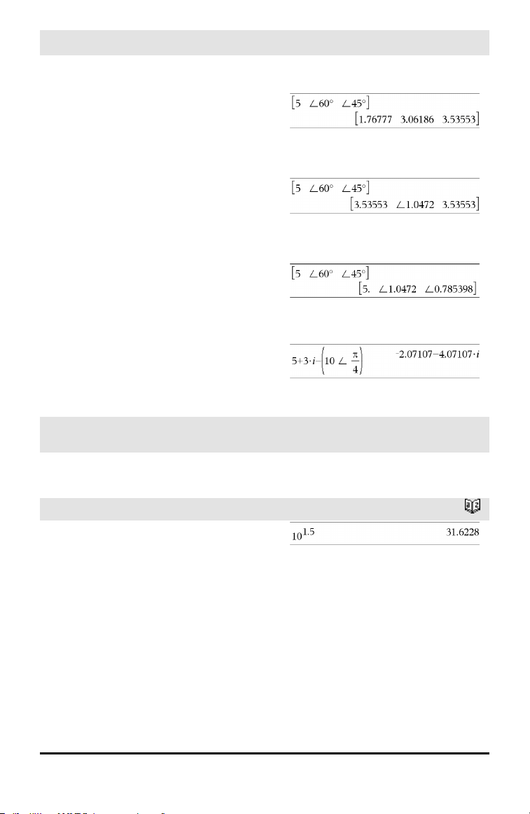
∠ (angle)
/k keys
[Radius,∠ θ_Angle] ⇒ vector
(polar input)
[Radius,∠ θ_Angle,Z_Coordinate] ⇒
vector
(cylindrical input)
[Radius,∠ θ_Angle,∠ θ_Angle] ⇒ vector
(spherical input)
Returns coordinates as a vector depending
on the Vector Format mode setting:
rectangular, cylindrical, or spherical.
Note: You can insert this symbol from the
computer keyboard by typing@<.
In Radian mode and vector format set to:
rectangular
cylindrical
spherical
(Magnitude∠ Angle) ⇒ complexValue
(polar input)
Enters a complex value in (r∠ θ) polar
form. The Angle is interpreted according to
the current Angle mode setting.
In Radian angle mode and Rectangular
complex format:
_ (underscore as an empty element)
See “Empty (Void) Elements,”
page 196.
10^()
Catalog >
10^ (Value1) ⇒ value
10^ (List1) ⇒ list
Returns 10 raised to the power of the
argument.
For a list, returns 10 raised to the power of
the elements in List1.
Symbols 191
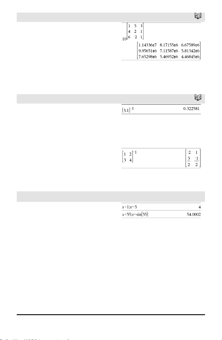
192 Symbols
10^()
Catalog >
10^(squareMatrix1) ⇒ squareMatrix
Returns 10 raised to the power of
squareMatrix1. This is not the same as
calculating 10 raised to the power of each
element. For information about the
calculation method, refer to cos().
squareMatrix1 must be diagonalizable. The
result always contains floating-point
numbers.
^⁻¹ (reciprocal)
Catalog >
Value1 ^⁻¹ ⇒ value
List1 ^⁻¹ ⇒ list
Returns the reciprocal of the argument.
For a list, returns the reciprocals of the
elements in List1.
squareMatrix1 ^⁻¹ ⇒ squareMatrix
Returns the inverse of squareMatrix1.
squareMatrix1 must be a non-singular
square matrix.
| (constraint operator)
/k keys
Expr | BooleanExpr1[and
BooleanExpr2]...
Expr | BooleanExpr1[orBooleanExpr2]...
The constraint (“|”) symbol serves as a
binary operator. The operand to the left of |
is an expression. The operand to the right of
| specifies one or more relations that are
intended to affect the simplification of the
expression. Multiple relations after | must
be joined by logical “and” or “or” operators.
The constraint operator provides three basic
types of functionality:
• Substitutions
• Interval constraints
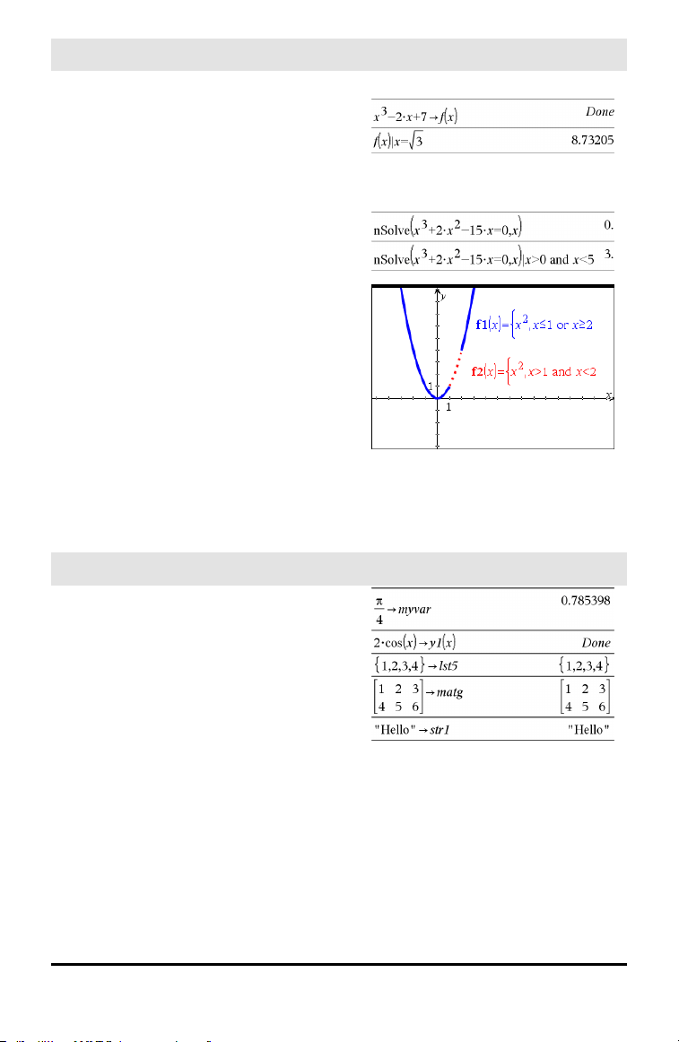
| (constraint operator)
/k keys
• Exclusions
Substitutions are in the form of an equality,
such as x=3 or y=sin(x). To be most
effective, the left side should be a simple
variable. Expr | Variable = value will
substitute value for every occurrence of
Variable in Expr.
Interval constraints take the form of one or
more inequalities joined by logical “and” or
“or” operators. Interval constraints also
permit simplification that otherwise might
be invalid or not computable.
Exclusions use the “not equals” (/= or ≠)
relational operator to exclude a specific
value from consideration.
→ (store)
/h key
Value → Var
List → Var
Matrix → Var
Expr → Function(Param1,...)
List → Function(Param1,...)
Matrix → Function(Param1,...)
If the variable Var does not exist, creates it
and initializes it to Value, List, or Matrix.
If the variable Var already exists and is not
locked or protected, replaces its contents
with Value, List, or Matrix.
Symbols 193
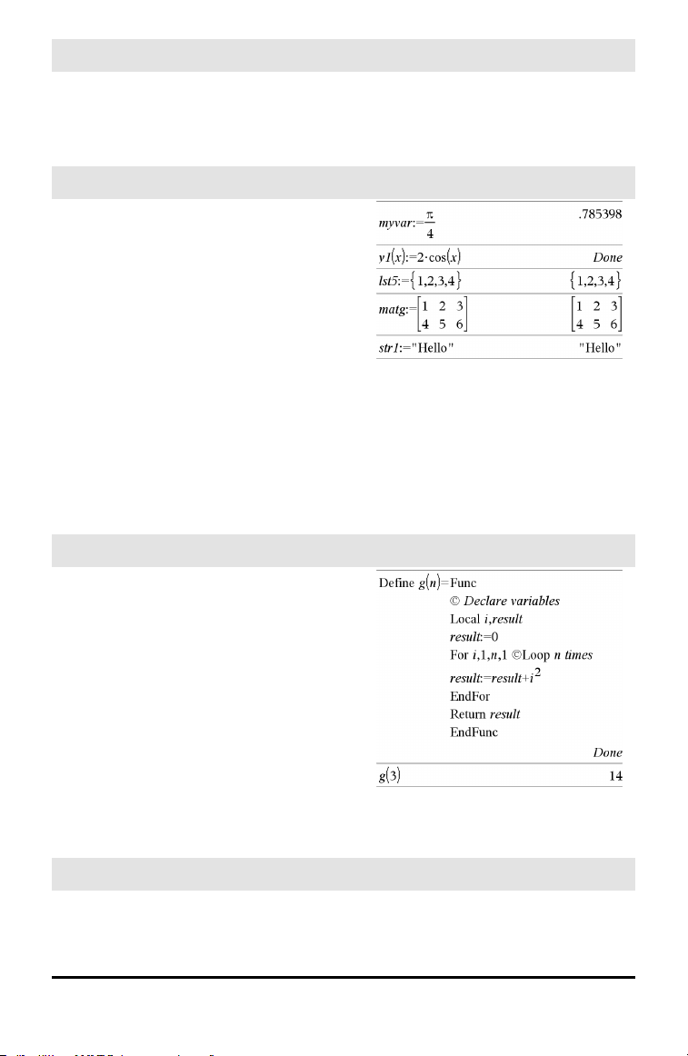
194 Symbols
→ (store)
/h key
Note: You can insert this operator from the
keyboard by typing =: as a shortcut. For
example, type pi/4 =: myvar.
:= (assign)
/t keys
Var := Value
Var := List
Var := Matrix
Function(Param1,...) := Expr
Function(Param1,...) := List
Function(Param1,...) := Matrix
If variable Var does not exist, creates Var
and initializes it to Value, List, or Matrix.
If Var already exists and is not locked or
protected, replaces its contents with Value,
List, or Matrix.
© (comment)
/k keys
© [text]
© processes text as a comment line,
allowing you to annotate functions and
programs that you create.
© can be at the beginning or anywhere in
the line. Everything to the right of ©, to the
end of the line, is the comment.
Note for entering the example: For
instructions on entering multi-line program
and function definitions, refer to the
Calculator section of your product
guidebook.
0b, 0h
0B keys, 0H keys
0b binaryNumber
0h hexadecimalNumber
In Dec base mode:

0b, 0h
0B keys, 0H keys
Denotes a binary or hexadecimal number,
respectively. To enter a binary or hex
number, you must enter the 0b or 0h prefix
regardless of the Base mode. Without a
prefix, a number is treated as decimal
(base10).
Results are displayed according to the Base
mode.
In Bin base mode:
In Hex base mode:
Symbols 195
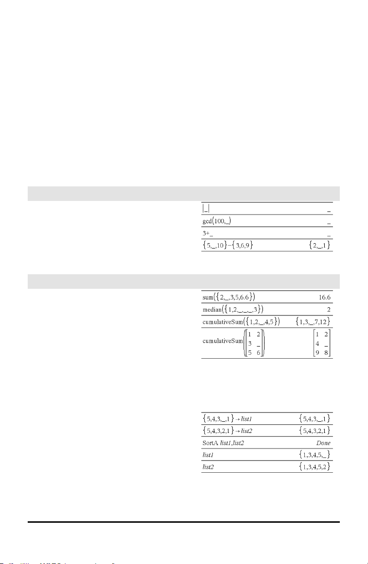
196 Empty (Void) Elements
Empty (Void) Elements
When analyzing real-world data, you might not always have a complete data set.
TI-Nspire™ Software allows empty, or void, data elements so you can proceed with the
nearly complete data rather than having to start over or discard the incomplete cases.
You can find an example of data involving empty elements in the Lists & Spreadsheet
chapter, under “Graphing spreadsheet data.”
The delVoid() function lets you remove empty elements from a list. The isVoid()
function lets you test for an empty element. For details, see delVoid(), page 38, and
isVoid(), page 74.
Note: To enter an empty element manually in a math expression, type “_” or the
keyword void. The keyword void is automatically converted to a “_” symbol when
the expression is evaluated. To type “_” on the handheld, press / _.
Calculations involving void elements
The majority of calculations involving a void
input will produce a void result. See special
cases below.
List arguments containing void elements
The following functions and commands
ignore (skip) void elements found in list
arguments.
count, countIf, cumulativeSum,
freqTable►list, frequency, max, mean,
median, product, stDevPop, stDevSamp,
sum, sumIf, varPop, and varSamp, as well as
regression calculations, OneVar, TwoVar,
and FiveNumSummary statistics, confidence
intervals, and stat tests
SortA and SortD move all void elements
within the first argument to the bottom.
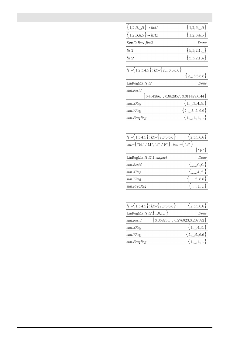
List arguments containing void elements
In regressions, a void in an X or Y list
introduces a void for the corresponding
element of the residual.
An omitted category in regressions
introduces a void for the corresponding
element of the residual.
A frequency of 0 in regressions introduces a
void for the corresponding element of the
residual.
Empty (Void) Elements 197

198 Shortcuts for Entering Math Expressions
Shortcuts for Entering Math Expressions
Shortcuts let you enter elements of math expressions by typing instead of using the
Catalog or Symbol Palette. For example, to enter the expression √6, you can type sqrt
(6) on the entry line. When you press ·, the expression sqrt(6) is changed to
√6. Some shortcuts are useful from both the handheld and the computer keyboard.
Others are useful primarily from the computer keyboard.
From the Handheld or Computer Keyboard
To enter this: Type this shortcut:
π pi
θ theta
∞
infinity
≤
<=
≥
>=
≠
/=
⇒ (logical implication) =>
⇔ (logical double implication, XNOR) <=>
→ (store operator) =:
|| (absolute value) abs(...)
√() sqrt(...)
Σ() (Sum template) sumSeq(...)
Π() (Product template) prodSeq(...)
sin⁻¹(), cos⁻¹(), ... arcsin(...), arccos(...), ...
ΔList() deltaList(...)
From the Computer Keyboard
To enter this: Type this shortcut:
i (imaginary constant) @i
e (natural log base e) @e
E (scientific notation) @E
T
(transpose) @t

To enter this: Type this shortcut:
r
(radians) @r
° (degrees) @d
g
(gradians) @g
∠ (angle) @<
► (conversion) @>
►Decimal, ►approxFraction(), and
so on.
@>Decimal, @>approxFraction(), and
so on.
Shortcuts for Entering Math Expressions 199

200 EOS™ (Equation Operating System) Hierarchy
EOS™ (Equation Operating System) Hierarchy
This section describes the Equation Operating System (EOS™) that is used by the
TI-Nspire™ math and science learning technology. Numbers, variables, and functions
are entered in a simple, straightforward sequence. EOS™ software evaluates
expressions and equations using parenthetical grouping and according to the priorities
described below.
Order of Evaluation
Level Operator
1 Parentheses (), brackets [], braces {}
2 Indirection (#)
3 Function calls
4 Post operators: degrees-minutes-seconds (°,',"), factorial (!), percentage
(%), radian (
r
), subscript ([]), transpose (
T
)
5 Exponentiation, power operator (^)
6 Negation (⁻)
7 String concatenation (&)
8 Multiplication (•), division (/)
9 Addition (+), subtraction (-)
10 Equality relations: equal (=), not equal (≠ or /=),
less than (<), less than or equal (≤ or <=), greater than (>), greater than or
equal (≥or>=)
11 Logical not
12 Logical and
13 Logical or
14 xor, nor, nand
15 Logical implication (⇒ )
16 Logical double implication, XNOR (⇔ )
17 Constraint operator (“|”)
18 Store (→)
Parentheses, Brackets, and Braces
All calculations inside a pair of parentheses, brackets, or braces are evaluated first. For
example, in the expression 4(1+2), EOS™ software first evaluates the portion of the
expression inside the parentheses, 1+2, and then multiplies the result, 3, by 4.

The number of opening and closing parentheses, brackets, and braces must be the
same within an expression or equation. If not, an error message is displayed that
indicates the missing element. For example, (1+2)/(3+4 will display the error message
“Missing ).”
Note: Because the TI-Nspire™ software allows you to define your own functions, a
variable name followed by an expression in parentheses is considered a “function call”
instead of implied multiplication. For example a(b+c) is the function a evaluated by
b+c. To multiply the expression b+c by the variable a, use explicit multiplication: a•
(b+c).
Indirection
The indirection operator (#) converts a string to a variable or function name. For
example, #(“x”&”y”&”z”) creates the variable name xyz. Indirection also allows the
creation and modification of variables from inside a program. For example, if 10→r
and “r”→s1, then #s1=10.
Post Operators
Post operators are operators that come directly after an argument, such as 5!, 25%, or
60°15' 45". Arguments followed by a post operator are evaluated at the fourth priority
level. For example, in the expression 4^3!, 3! is evaluated first. The result, 6, then
becomes the exponent of 4 to yield 4096.
Exponentiation
Exponentiation (^) and element-by-element exponentiation (.^) are evaluated from
right to left. For example, the expression 2^3^2 is evaluated the same as 2^(3^2) to
produce 512. This is different from (2^3)^2, which is 64.
Negation
To enter a negative number, press v followed by the number. Post operations and
exponentiation are performed before negation. For example, the result of −x
2
is a
negative number, and −9
2
= −81. Use parentheses to square a negative number such
as (−9)
2
to produce 81.
Constraint (“|”)
The argument following the constraint (“|”) operator provides a set of constraints that
affect the evaluation of the argument preceding the operator.
EOS™ (Equation Operating System) Hierarchy 201

202 Constants and Values
Constants and Values
The following table lists the constants and their values that are available when
performing unit conversions. They can be typed in manually or selected from the
Constants list in Utilities > Unit Conversions (Handheld: Press k 3).
Constant Name Value
_c Speed of light 299792458 _m/_s
_Cc Coulomb constant 8987551787.3682 _m/_F
_Fc Faraday constant 96485.33289 _coul/_mol
_g Acceleration of gravity 9.80665 _m/_s
2
_Gc Gravitational constant 6.67408E-11 _m
3
/_kg/_s
2
_h Planck's constant 6.626070040E-34 _J _s
_k Boltzmann's constant 1.38064852E-23 _J/_¡K
_m0 Permeability of a vacuum 1.2566370614359E-6 _N/_A
2
_mb Bohr magneton 9.274009994E-24 _J _m
2
/_Wb
_Me Electron rest mass 9.10938356E-31 _kg
_Mm Muon mass 1.883531594E-28 _kg
_Mn Neutron rest mass 1.674927471E-27 _kg
_Mp Proton rest mass 1.672621898E-27 _kg
_Na Avogadro's number 6.022140857E23 /_mol
_q Electron charge 1.6021766208E-19 _coul
_Rb Bohr radius 5.2917721067E-11 _m
_Rc Molar gas constant 8.3144598 _J/_mol/_¡K
_Rdb Rydberg constant 10973731.568508/_m
_Re Electron radius 2.8179403227E-15 _m
_u Atomic mass 1.660539040E-27 _kg
_Vm Molar volume 2.2413962E-2 _m
3
/_mol
_H0 Permittivity of a vacuum 8.8541878176204E-12 _F/_m
_s Stefan-Boltzmann constant 5.670367E-8 _W/_m
2
/_¡K
4
_f0 Magnetic flux quantum 2.067833831E-15 _Wb

Error Codes and Messages
When an error occurs, its code is assigned to variable errCode. User-defined programs
and functions can examine errCode to determine the cause of an error. For an
example of using errCode, See Example 2 under the Try command, page 157.
Note: Some error conditions apply only to TI-Nspire™CAS products, and some apply
only to TI-Nspire™ products.
Error
code
Description
10 A function did not return a value
20 A testdid not resolve to TRUE or FALSE.
Generally, undefined variables cannot be compared. For example, the test If a<bwill cause
this error if either a or b is undefined when the If statement is executed.
30 Argument cannot be a folder name.
40 Argument error
50 Argument mismatch
Two or more arguments must be of the same type.
60 Argument must be a Boolean expression or integer
70 Argument must be a decimal number
90 Argument must be a list
100 Argument must be a matrix
130 Argument must be a string
140 Argument must be a variable name.
Make sure that the name:
• does not begin with a digit
• does not contain spaces or special characters
• does not use underscore or period in invalid manner
• does not exceed the length limitations
See the Calculator section in the documentation for more details.
160 Argument must be an expression
165 Batteries too low for sending or receiving
Install new batteries before sending or receiving.
170 Bound
The lower boundmust be less than the upper bound to define the search interval.
Error Codes and Messages 203

204 Error Codes and Messages
Error
code
Description
180 Break
The d or c key was pressedduring a long calculation or during program execution.
190 Circular definition
This message is displayed to avoid running out of memory during infinite replacement of
variable values during simplification. For example, a+1->a, where a is an undefinedvariable,
will cause this error.
200 Constraint expression invalid
For example, solve(3x^2-4=0,x) | x<0 or x>5 would produce this error message because the
constraintis separated by “or” instead of “and.”
210 Invalid Data type
An argument is of the wrong data type.
220 Dependentlimit
230 Dimension
A listor matrix index is not valid. For example, if the list {1,2,3,4} is stored in L1, then L1[5] is a
dimension error because L1 only contains four elements.
235 Dimension Error. Not enough elements inthe lists.
240 Dimension mismatch
Two or more arguments must be of the same dimension. For example, [1,2]+[1,2,3] is a
dimension mismatch because the matrices contain a different number of elements.
250 Divide by zero
260 Domain error
An argument must be ina specifieddomain. For example, rand(0) is not valid.
270 Duplicate variable name
280 Else and ElseIf invalid outside of If...EndIf block
290 EndTry is missing the matching Else statement
295 Excessive iteration
300 Expected2 or 3-element list or matrix
310 The first argument of nSolve mustbe an equation in a single variable. It cannot contain a non-
valuedvariable other than the variable of interest.
320 First argumentof solve or cSolve must be an equation or inequality
For example, solve(3x^2-4,x) is invalid because the first argument is not an equation.

Error
code
Description
345 Inconsistent units
350 Index out of range
360 Indirection string is not a valid variable name
380 Undefined Ans
Either the previous calculation did not create Ans, or no previous calculation was entered.
390 Invalid assignment
400 Invalid assignmentvalue
410 Invalid command
430 Invalid for the current mode settings
435 Invalid guess
440 Invalid implied multiply
For example, x(x+1) is invalid; whereas, x*(x+1) is the correct syntax. This is to avoid
confusion between implied multiplication and function calls.
450 Invalid ina function or current expression
Only certaincommands are valid in a user-defined function.
490 Invalid inTry..EndTry block
510 Invalid listor matrix
550 Invalid outside function or program
A number of commands are not valid outside a function or program. For example, Local
cannot be used unless it is ina function or program.
560 Invalid outside Loop..EndLoop, For..EndFor, or While..EndWhile blocks
For example, the Exit command is validonly inside these loop blocks.
565 Invalid outside program
570 Invalid pathname
For example, \var is invalid.
575 Invalid polar complex
580 Invalid program reference
Programs cannot be referenced within functions or expressions such as 1+p(x) where p is a
program.
Error Codes and Messages 205

206 Error Codes and Messages
Error
code
Description
600 Invalid table
605 Invalid use of units
610 Invalid variable name in a Local statement
620 Invalid variable or function name
630 Invalid variable reference
640 Invalid vector syntax
650 Link transmission
A transmission between two units was not completed. Verify that the connecting cable is
connected firmly to both ends.
665 Matrix not diagonalizable
670 Low Memory
1. Delete some data in this document
2. Save andclose this document
If 1 and2 fail, pull outand re-insert batteries
672 Resource exhaustion
673 Resource exhaustion
680 Missing (
690 Missing )
700 Missing “
710 Missing ]
720 Missing }
730 Missing start or end of block syntax
740 Missing Thenin the If..EndIf block
750 Name is not a function or program
765 No functions selected
780 No solution found
800 Non-real result
For example, if the software is in the Real setting, √(-1) is invalid.

Error
code
Description
To allow complex results, change the “Real or Complex” Mode Setting to RECTANGULAR or
POLAR.
830 Overflow
850 Program not found
A program reference inside another program could not be found in the provided path during
execution.
855 Rand type functions not allowed ingraphing
860 Recursion too deep
870 Reserved name or system variable
900 Argument error
Median-median model could not be appliedto data set.
910 Syntax error
920 Text not found
930 Too fewarguments
The function or command is missing one or more arguments.
940 Too many arguments
The expression or equation contains an excessive number of arguments andcannot be
evaluated.
950 Too many subscripts
955 Too many undefined variables
960 Variable is not defined
No value is assigned to variable. Use one of the following commands:
• sto →
• :=
• Define
to assign values to variables.
965 Unlicensed OS
970 Variable inuse so references or changes are not allowed
980 Variable is protected
990 Invalid variable name
Make sure that the name does not exceed the lengthlimitations
Error Codes and Messages 207

208 Error Codes and Messages
Error
code
Description
1000 Window variables domain
1010 Zoom
1020 Internal error
1030 Protected memory violation
1040 Unsupportedfunction. This function requires Computer Algebra System. Try TI-Nspire™
CAS.
1045 Unsupportedoperator. This operator requires Computer Algebra System. Try TI-Nspire™
CAS.
1050 Unsupportedfeature. This operator requires Computer Algebra System. Try TI-Nspire™
CAS.
1060 Input argumentmust be numeric. Only inputs containing numeric values are allowed.
1070 Trig function argument too big for accurate reduction
1080 Unsupporteduse of Ans.This application does not support Ans.
1090 Function is not defined. Use one of the following commands:
• Define
• :=
• sto →
to define a function.
1100 Non-real calculation
For example, if the software is in the Real setting, √(-1) is invalid.
To allow complex results, change the “Real or Complex” Mode Setting to RECTANGULAR or
POLAR.
1110 Invalid bounds
1120 No sign change
1130 Argument cannot be a list or matrix
1140 Argument error
The first argument must be a polynomial expression inthe secondargument. If the second
argument is omitted, the software attempts to selecta default.
1150 Argument error
The first two arguments must be polynomial expressions in the third argument. If the third
argument is omitted, the software attempts to selecta default.
1160 Invalid library pathname

Error
code
Description
A pathname must be in the form xxx\yyy, where:
• The xxx part can have 1 to 16 characters.
• The yyy part can have 1 to 15 characters.
See the Library section in the documentation for more details.
1170 Invalid use of library pathname
• A value cannot be assigned to a pathname using Define, :=, or sto →.
• A pathname cannot be declared as a Local variable or be used as a
parameter in a function or program definition.
1180 Invalid library variable name.
Make sure that the name:
• Does not contain a period
• Does not begin with an underscore
• Does not exceed 15 characters
See the Library section in the documentation for more details.
1190 Library document not found:
• Verify library is in the MyLib folder.
• Refresh Libraries.
See the Library section in the documentation for more details.
1200 Library variable not found:
• Verify library variable exists in the first problem in the library.
• Make sure library variable has been defined as LibPub or LibPriv.
• Refresh Libraries.
See the Library section in the documentation for more details.
1210 Invalid library shortcutname.
Make sure that the name:
• Does not contain a period
• Does not begin with an underscore
• Does not exceed 16 characters
• Is not a reserved name
See the Library section in the documentation for more details.
1220 Domain error:
The tangentLine and normalLine functions support real-valuedfunctions only.
1230 Domain error.
Error Codes and Messages 209

210 Error Codes and Messages
Error
code
Description
Trigonometric conversion operators are not supported in Degree or Gradian angle modes.
1250 Argument Error
Use a system of linear equations.
Example of a system of two linear equations with variables x and y:
3x+7y=5
2y-5x=-1
1260 Argument Error:
The first argument of nfMin or nfMax must be an expression in a single variable. It cannot
contain a non-valued variable other than the variable of interest.
1270 Argument Error
Order of the derivative must be equal to 1 or 2.
1280 Argument Error
Use a polynomial in expanded form inone variable.
1290 Argument Error
Use a polynomial in one variable.
1300 Argument Error
The coefficients of the polynomial mustevaluate to numeric values.
1310 Argument error:
A function couldnot be evaluatedfor one or more of its arguments.
1380 Argument error:
Nested calls to domain() function are not allowed.

Warning Codes and Messages
You can use the warnCodes() function to store the codes of warnings generated by
evaluating an expression. This table lists each numeric warning code and its associated
message. For an example of storing warning codes, see warnCodes(), page 165.
Warning
code Message
10000 Operation mightintroduce false solutions.
10001 Differentiating an equation may produce a false equation.
10002 Questionable solution
10003 Questionable accuracy
10004 Operation mightlose solutions.
10005 cSolve mightspecify more zeros.
10006 Solve may specify more zeros.
10007 More solutions may exist. Try specifying appropriate lower andupper bounds and/or a
guess.
Examples using solve():
• solve(Equation, Var=Guess)|lowBound<Var<upBound
• solve(Equation, Var)|lowBound<Var<upBound
• solve(Equation, Var=Guess)
10008 Domain of the result might be smaller than the domain of the input.
10009 Domain of the result might be larger than the domain of the input.
10012 Non-real calculation
10013
∞^0 or undef^0 replaced by 1
10014 undef^0 replaced by 1
10015
1^∞ or 1^undef replaced by 1
10016 1^undef replaced by 1
10017
Overflow replaced by ∞ or −∞
10018 Operation requires and returns 64 bit value.
10019 Resource exhaustion, simplification mightbe incomplete.
10020 Trig function argumenttoo big for accurate reduction.
10021 Input contains an undefinedparameter.
Resultmight not be validfor all possible parameter values.
Warning Codes and Messages 211

212 Warning Codes and Messages
Warning
code Message
10022 Specifying appropriate lower andupper bounds might produce a solution.
10023 Scalar has been multipliedby the identity matrix.
10024 Result obtained using approximate arithmetic.
10025 Equivalence cannot be verified in EXACT mode.
10026 Constraint mightbe ignored. Specify constraintin the form "\" 'Variable MathTestSymbol
Constant' or a conjunct of these forms, for example 'x<3 and x>-12'

Support and Service
Texas Instruments Support and Service
General Information: North and South America
Home Page:
education.ti.com
KnowledgeBase and e-mail inquiries:
education.ti.com/support
Phone: (800) TI-CARES / (800) 842-2737
For North and South America and U.S.
Territories
International contact information:
https://education.ti.com/en/us/customer-
support/support_worldwide
For Technical Support
Knowledge Base and support by e-mail:
education.ti.com/support or ti-
cares@ti.com
Phone (not toll-free): (972) 917-8324
For Product (Hardware) Service
Customers in the U.S., Canada, Mexico, and U.S. territories: Always contact Texas
Instruments Customer Support before returning a product for service.
For All Other Countries:
For general information
For more information about TI products and services, contact TI by e-mail or visit the
TIInternet address.
E-mail inquiries:
ti-cares@ti.com
Home Page:
education.ti.com
Service and Warranty Information
For information about the length and terms of the warranty or about product service,
refer to the warranty statement enclosed with this product or contact your local Texas
Instruments retailer/distributor.
Support and Service 213

Index
-
-, subtract
173
!
!, factorial
183
"
", second notation
190
#
#, indirection
188
#, indirection operator
201
%
%, percent
179
&
&, append
183
*
*, multiply
174
.
.-, dot subtraction
177
.*, dot multiplication
178
./, dot division
178
.^, dot power
178
.+, dot addition
177
/
/, divide
175
:
:=, assign
194
^
^⁻¹, reciprocal
192
^, power
176
|
|, constraint operator
192
′
′ minute notation
190
+
+, add
173
=
≠, not equal
180
≤, less than or equal
181
≥, greater than or equal
182
>, greater than
181
=, equal
179
∏
∏, product
185
∑
∑(), sum
186
∑Int()
186
∑Prn()
187
√
√, square root
185
∠
∠ (angle)
191
∫
∫, integral
185
►
►approxFraction()
12
►Base10, display as decimal integer
17
►Base16, display as hexadecimal
17
►Base2, display as binary
16
Index 214

►Cylind, display as cylindrical vector
34
►DD, display as decimal angle
35
►Decimal, display result as decimal
35
►DMS, display as
degree/minute/second
42
►Grad, convert to gradian angle
67
►Polar, display as polar vector
110
►Rad, convert to radian angle
119
►Rect, display as rectangular vector
122
►Sphere, display as spherical vector
144
⇒
⇒ , logical implication
182, 198
→
→, store variable
193
⇔
⇔ , logical double implication
183, 198
©
©, comment
194
°
°, degree notation
190
°, degrees/minutes/seconds
190
0
0b, binary indicator
194
0h, hexadecimalindicator
194
1
10^(), power of ten
191
2
2-sample F Test
56
A
abs(), absolute value
7
absolute value
template for
3-4
add, +
173
amortization table, amortTbl()
7, 15
amortTbl(), amortization table
7, 15
and, Boolean operator
8
angle(), angle
8
angle, angle()
8
ANOVA, one-way variance analysis
9
ANOVA2way, two-way variance
analysis
10
Ans, last answer
12
answer (last), Ans
12
append, &
183
approx(), approximate
12
approximate, approx()
12
approxRational()
13
arccos(), cos⁻¹()
13
arccosh(), cosh⁻¹()
13
arccot(), cot⁻¹()
13
arccoth(), coth⁻¹()
13
arccsc(), csc⁻¹()
13
arccsch(), csch⁻¹()
13
arcsec(), sec⁻¹()
14
arcsech(), csech⁻¹()
14
arcsin(), sin⁻¹()
14
arcsinh(), sinh⁻¹()
14
arctan(), tan⁻¹()
14
arctanh(), tanh⁻¹()
14
arguments in TVM functions
161
augment(), augment/concatenate
14
augment/concatenate, augment()
14
average rate of change, avgRC()
15
avgRC(), average rate of change
15
B
binary
display, ►Base2
16
indicator, 0b
194
binomCdf()
18, 72
binomPdf()
18
Boolean operators
⇒
182, 198
⇔
183
and
8
nand
98
215 Index

nor
102
not
103
or
107
xor
166
C
Cdf()
51
ceiling(), ceiling
19
ceiling, ceiling()
19, 30
centralDiff()
19
char(), character string
20
character string, char()
20
characters
numeric code, ord()
108
string, char()
20
χ²2way
20
clear
error, ClrErr
22
ClearAZ
22
ClrErr, clear error
22
colAugment
23
colDim(), matrix column dimension
23
colNorm(), matrix column norm
23
combinations, nCr()
99
comment, ©
194
complex
conjugate, conj()
23
conj(), complex conjugate
23
constraint operator "|"
192
constraint operator, order of
evaluation
200
construct matrix, constructMat()
24
constructMat(), construct matrix
24
convert
►Grad
67
►Rad
119
copy variable or function, CopyVar
24
correlation matrix, corrMat()
25
corrMat(), correlation matrix
25
cos⁻¹, arccosine
26
cos(), cosine
25
cosh⁻¹(), hyperbolic arccosine
27
cosh(), hyperbolic cosine
26
cosine, cos()
25
cot⁻¹(), arccotangent
28
cot(), cotangent
28
cotangent, cot()
28
coth⁻¹(), hyperbolic arccotangent
29
coth(), hyperbolic cotangent
28
count days between dates, dbd()
34
count items in a list conditionally ,
countif()
29
count items in a list, count()
29
count(), count items in a list
29
countif(), conditionally count items
in a list
29
cPolyRoots()
30
cross product, crossP()
30
crossP(), cross product
30
csc⁻¹(), inverse cosecant
31
csc(), cosecant
31
csch⁻¹(), inverse hyperbolic cosecant
32
csch(), hyperbolic cosecant
32
cubic regression, CubicReg
32
CubicReg, cubic regression
32
cumulative sum, cumulativeSum()
33
cumulativeSum(), cumulative sum
33
cycle, Cycle
34
Cycle, cycle
34
cylindrical vector display, ►Cylind
34
D
d(), first derivative
184
days between dates, dbd()
34
dbd(), days between dates
34
decimal
angle display, ►DD
35
integer display, ►Base10
17
Define
35
Define LibPriv
37
Define LibPub
37
define, Define
35
Define, define
35
defining
private function or program
37
public function or program
37
Index 216

definite integral
template for
6
degree notation, °
190
degree/minute/second display,
►DMS
42
degree/minute/second notation
190
delete
void elements from list
38
deleting
variable, DelVar
38
deltaList()
38
DelVar, delete variable
38
delVoid(), remove void elements
38
derivatives
first derivative, d()
184
numeric derivative, nDeriv()
100-101
numeric derivative, nDerivative(
)
99
det(), matrix determinant
39
diag(), matrix diagonal
39
dim(), dimension
39
dimension, dim()
39
Disp, display data
40, 134
DispAt
40
display as
binary, ►Base2
16
cylindrical vector, ►Cylind
34
decimalangle, ►DD
35
decimalinteger, ►Base10
17
degree/minute/second, ►DMS
42
hexadecimal, ►Base16
17
polar vector, ►Polar
110
rectangular vector, ►Rect
122
sphericalvector, ►Sphere
144
display data, Disp
40, 134
distribution functions
binomCdf()
18, 72
binomPdf()
18
invNorm()
73
invt()
73
Invχ²()
71
normCdf()
103
normPdf()
103
poissCdf()
110
poissPdf()
110
tCdf()
153
tPdf()
156
χ²2way()
20
χ²Cdf()
20
χ²GOF()
21
χ²Pdf()
21
divide, /
175
dot
addition, .+
177
division, ./
178
multiplication, .*
178
power, .^
178
product, dotP()
43
subtraction, .-
177
dotP(), dot product
43
E
e exponent
template for
2
e to a power, e^()
43, 48
E, exponent
188
e^(), e to a power
43
eff(), convert nominal to effective
rate
44
effective rate, eff()
44
eigenvalue, eigVl()
44
eigenvector, eigVc()
44
eigVc(), eigenvector
44
eigVl(), eigenvalue
44
else if, ElseIf
45
else, Else
67
ElseIf, elseif
45
empty (void) elements
196
end
for, EndFor
53
function, EndFunc
57
if, EndIf
67
loop, EndLoop
89
program, EndPrgm
113
try, EndTry
157
while, EndWhile
166
end function, EndFunc
57
end if, EndIf
67
end loop, EndLoop
89
217 Index

end while, EndWhile
166
EndTry, end try
157
EndWhile, end while
166
EOS (Equation Operating System)
200
equal, =
179
Equation Operating System (EOS)
200
error codes and messages
203, 211
errors and troubleshooting
clear error, ClrErr
22
pass error, PassErr
109
euler(), Euler function
46
evaluate polynomial, polyEval()
111
evaluation, order of
200
exclusion with "|" operator
192
exit, Exit
48
Exit, exit
48
exp(), e to a power
48
exponent, E
188
exponentialregession, ExpReg
49
exponents
template for
1
expr(), string to expression
49
ExpReg, exponential regession
49
expressions
string to expression, expr()
49
F
factor(), factor
50
factor, factor()
50
factorial, !
183
Fill, matrix fill
51
financial functions, tvmFV()
159
financial functions, tvmI()
159
financial functions, tvmN()
160
financial functions, tvmPmt()
160
financial functions, tvmPV()
160
first derivative
template for
5
FiveNumSummary
52
floor(), floor
52
floor, floor()
52
For
53
for, For
53
For, for
53
format string, format()
53
format(), format string
53
fpart(), function part
54
fractions
propFrac
114
template for
1
freqTable()
55
frequency()
55
Frobenius norm, norm()
103
Func, function
57
Func, program function
57
functions
part, fpart()
54
program function, Func
57
user-defined
35
functions and variables
copying
24
G
g, gradians
189
gcd(), greatest common divisor
57
geomCdf()
58
geomPdf()
58
Get
58
get/return
denominator, getDenom()
59
number, getNum()
65
variables injformation,
getVarInfo()
63, 66
getDenom(), get/return
denominator
59
getKey()
60
getLangInfo(), get/return language
information
63
getLockInfo(), tests lock status of
variable or variable group
63
getMode(), get mode settings
64
getNum(), get/return number
65
GetStr
65
getType(), get type of variable
65
getVarInfo(), get/return variables
information
66
go to, Goto
67
Index 218

Goto, go to
67
gradian notation, g
189
greater than or equal, ≥
182
greater than, >
181
greatest common divisor, gcd()
57
groups, locking and unlocking
85, 163
groups, testing lock status
63
H
hexadecimal
display, ►Base16
17
indicator, 0h
194
hyperbolic
arccosine, cosh⁻¹()
27
arcsine, sinh⁻¹()
142
arctangent, tanh⁻¹()
153
cosine, cosh()
26
sine, sinh()
141
tangent, tanh()
152
I
identity matrix, identity()
67
identity(), identity matrix
67
if, If
67
If, if
67
ifFn()
69
imag(), imaginary part
69
imaginary part, imag()
69
indirection operator (#)
201
indirection, #
188
inString(), within string
70
int(), integer
70
intDiv(), integer divide
71
integer divide, intDiv()
71
integer part, iPart()
73
integer, int()
70
integral, ∫
185
interpolate(), interpolate
71
inverse cumulative normal
distribution (invNorm()
73
inverse, ^⁻¹
192
invF()
72
invNorm(), inverse cumulative
73
normal distribution)
invt()
73
Invχ²()
71
iPart(), integer part
73
irr(), internal rate of return
internal rate of return, irr()
73
isPrime(), prime test
74
isVoid(), test for void
74
L
label, Lbl
75
language
get language information
63
Lbl, label
75
lcm, least common multiple
75
least common multiple, lcm
75
left(), left
75
left, left()
75
length of string
39
less than or equal, ≤
181
LibPriv
37
LibPub
37
library
create shortcuts to objects
76
libShortcut(), create shortcuts to
library objects
76
linear regression, LinRegAx
77
linear regression, LinRegBx
76, 78
LinRegBx, linear regression
76
LinRegMx, linear regression
77
LinRegtIntervals, linear regression
78
LinRegtTest
80
linSolve()
81
Δlist(), list difference
82
list to matrix, list►mat()
82
list, conditionally count items in
29
list, count items in
29
list►mat(), list to matrix
82
lists
augment/concatenate,
augment()
14
cross product, crossP()
30
cumulative sum,
cumulativeSum()
33
219 Index

differences in a list, Δlist()
82
dot product, dotP()
43
empty elements in
196
list to matrix, list►mat()
82
matrix to list, mat►list()
90
maximum, max()
90
mid-string, mid()
93
minimum, min()
93
new, newList()
100
product, product()
114
sort ascending, SortA
144
sort descending, SortD
144
summation, sum()
149
ln(), natural logarithm
82
LnReg, logarithmic regression
83
local variable, Local
85
local, Local
85
Local, localvariable
85
Lock, lock variable or variable group
85
locking variables and variablegroups
85
Log
template for
2
logarithmic regression, LnReg
83
logarithms
82
logical double implication, ⇔
183
logical implication, ⇒
182, 198
logistic regression, Logistic
86
logistic regression, LogisticD
87
Logistic, logistic regression
86
LogisticD, logistic regression
87
loop, Loop
89
Loop, loop
89
LU, matrix lower-upper
decomposition
89
M
mat►list(), matrix to list
90
matrices
augment/concatenate,
augment()
14
column dimension, colDim()
23
column norm, colNorm()
23
cumulative sum,
cumulativeSum()
33
determinant, det()
39
diagonal, diag()
39
dimension, dim()
39
dot addition, .+
177
dot division, ./
178
dot multiplication, .*
178
dot power, .^
178
dot subtraction, .-
177
eigenvalue, eigVl()
44
eigenvector, eigVc()
44
filling, Fill
51
identity, identity()
67
list to matrix, list►mat()
82
lower-upper decomposition, LU
89
matrix to list, mat►list()
90
maximum, max()
90
minimum, min()
93
new, newMat()
100
product, product()
114
QR factorization, QR
115
random, randMat()
120
reduced row echelon form, rref(
)
132
row addition, rowAdd()
131
row dimension, rowDim()
131
row echelon form, ref()
122
row multiplication and addition,
mRowAdd()
95
row norm, rowNorm()
131
row operation, mRow()
95
row swap, rowSwap()
132
submatrix, subMat()
149-150
summation, sum()
149
transpose, T
151
matrix (1× 2)
template for
4
matrix (2× 1)
template for
4
matrix (2× 2)
template for
4
matrix (m × n)
template for
4
matrix to list, mat►list()
90
max(), maximum
90
Index 220

maximum, max()
90
mean(), mean
91
mean, mean()
91
median(), median
91
median, median()
91
medium-medium line regression,
MedMed
92
MedMed, medium-medium line
regression
92
mid-string, mid()
93
mid(), mid-string
93
min(), minimum
93
minimum, min()
93
minute notation, ′
190
mirr(), modified internal rate of
return
94
mixed fractions, using propFrac(›
with
114
mod(), modulo
94
mode settings, getMode()
64
modes
setting, setMode()
136
modified internal rate of return, mirr
()
94
modulo, mod()
94
mRow(), matrix row operation
95
mRowAdd(), matrix row
multiplication and addition
95
Multiple linear regression t test
97
multiply, *
174
MultReg
95
MultRegIntervals()
96
MultRegTests()
97
N
nand, Boolean operator
98
natural logarithm, ln()
82
nCr(), combinations
99
nDerivative(), numeric derivative
99
negation, entering negative numbers
201
net present value, npv()
105
new
list, newList()
100
matrix, newMat()
100
newList(), new list
100
newMat(), new matrix
100
nfMax(), numeric function
maximum
100
nfMin(), numeric function minimum
101
nInt(), numeric integral
101
nom ), convert effective to nominal
rate
102
nominalrate, nom()
102
nor, Boolean operator
102
norm(), Frobenius norm
103
normal distribution probability,
normCdf()
103
normCdf()
103
normPdf()
103
not equal, ≠
180
not, Boolean operator
103
nPr(), permutations
104
npv(), net present value
105
nSolve(), numeric solution
105
nth root
template for
1
numeric
derivative, nDeriv()
100-101
derivative, nDerivative()
99
integral, nInt()
101
solution, nSolve()
105
O
objects
create shortcuts to library
76
one-variable statistics, OneVar
106
OneVar, one-variable statistics
106
operators
order of evaluation
200
or (Boolean), or
107
or, Boolean operator
107
ord(), numeric character code
108
P
P►Rx(), rectangular x coordinate
108
P►Ry(), rectangular y coordinate
109
pass error, PassErr
109
PassErr, pass error
109
Pdf()
54
221 Index

percent, %
179
permutations, nPr()
104
piecewise function (2-piece)
template for
2
piecewise function (N-piece)
template for
2
piecewise()
110
poissCdf()
110
poissPdf()
110
polar
coordinate, R►Pr()
118
coordinate, R►Pθ()
118
vector display, ►Polar
110
polyEval(), evaluate polynomial
111
polynomials
evaluate, polyEval()
111
random, randPoly()
121
PolyRoots()
112
power of ten, 10^()
191
power regression,
PowerReg
112, 125-126, 154
power, ^
176
PowerReg, power regression
112
Prgm, define program
113
prime number test, isPrime()
74
probability densiy, normPdf()
103
prodSeq()
114
product(), product
114
product, ∏()
185
template for
5
product, product()
114
programming
define program, Prgm
113
display data, Disp
40, 134
pass error, PassErr
109
programs
defining private library
37
defining public library
37
programs and programming
clear error, ClrErr
22
display I/O screen, Disp
40, 134
end program, EndPrgm
113
end try, EndTry
157
try, Try
157
proper fraction, propFrac
114
propFrac, proper fraction
114
Q
QR factorization, QR
115
QR, QR factorization
115
quadratic regression, QuadReg
116
QuadReg, quadratic regression
116
quartic regression, QuartReg
117
QuartReg, quartic regression
117
R
R, radian
189
R►Pr(), polar coordinate
118
R►Pθ(), polar coordinate
118
radian, R
189
rand(), random number
119
randBin, random number
119
randInt(), random integer
120
randMat(), random matrix
120
randNorm(), random norm
120
random
matrix, randMat()
120
norm, randNorm()
120
number seed, RandSeed
121
polynomial, randPoly()
121
random sample
121
randPoly(), random polynomial
121
randSamp()
121
RandSeed, random number seed
121
real(), real
121
real, real()
121
reciprocal, ^⁻¹
192
rectangular-vector display, ►Rect
122
rectangular x coordinate, P►Rx()
108
rectangular y coordinate, P►Ry()
109
reduced row echelon form, rref()
132
ref(), row echelon form
122
RefreshProbeVars
123
regressions
cubic, CubicReg
32
exponential, ExpReg
49
linear regression, LinRegAx
77
Index 222

linear regression, LinRegBx
76, 78
logarithmic, LnReg
83
Logistic
86
logistic, Logistic
87
medium-medium line, MedMed
92
MultReg
95
power regression,
PowerReg
112, 125-126, 154
quadratic, QuadReg
116
quartic, QuartReg
117
sinusoidal, SinReg
142
remain(), remainder
124
remainder, remain()
124
remove
void elements from list
38
Request
125
RequestStr
126
result values, statistics
146
results, statistics
145
return, Return
127
Return, return
127
right(), right
127
right, right()
46, 71, 127-128
rk23(), Runge Kutta function
128
rotate(), rotate
129
rotate, rotate()
129
round(), round
130
round, round()
130
row echelon form, ref()
122
rowAdd(), matrix row addition
131
rowDim(), matrix row dimension
131
rowNorm(), matrix row norm
131
rowSwap(), matrix row swap
132
rref(), reduced row echelon form
132
S
sec⁻¹(), inversesecant
133
sec(), secant
132
sech⁻¹(), inverse hyperbolic secant
133
sech(), hyperbolic secant
133
second derivative
template for
5
second notation, "
190
seq(), sequence
134
seqGen()
135
seqn()
135
sequence, seq()
134-135
set
mode, setMode()
136
setMode(), set mode
136
settings, get current
64
shift(), shift
137
shift, shift()
137
sign(), sign
139
sign, sign()
139
simult(), simultaneous equations
139
simultaneous equations, simult()
139
sin⁻¹(), arcsine
141
sin(), sine
140
sine, sin()
140
sinh⁻¹(), hyperbolic arcsine
142
sinh(), hyperbolic sine
141
SinReg, sinusoidal regression
142
sinusoidal regression, SinReg
142
SortA, sort ascending
144
SortD, sort descending
144
sorting
ascending, SortA
144
descending, SortD
144
sphericalvector display, ►Sphere
144
sqrt(), square root
145
square root
template for
1
square root, √()
145, 185
standard deviation, stdDev()
147, 163
stat.results
145
stat.values
146
statistics
combinations, nCr()
99
factorial, !
183
mean, mean()
91
median, median()
91
one-variable statistics, OneVar
106
permutations, nPr()
104
random norm, randNorm()
120
random number seed,
RandSeed
121
standard deviation, stdDev()
147, 163
223 Index

two-variableresults, TwoVar
161
variance, variance()
164
stdDevPop(), population standard
deviation
147
stdDevSamp(), sample standard
deviation
147
Stop command
148
store variable (→)
193
storing
symbol, &
194
string
dimension, dim()
39
length
39
string(), expression to string
148
strings
append, &
183
character code, ord()
108
character string, char()
20
expression to string, string()
148
format, format()
53
formatting
53
indirection, #
188
left, left()
75
mid-string, mid()
93
right, right()
46, 71, 127-128
rotate, rotate()
129
shift, shift()
137
string to expression, expr()
49
using to create variable names
201
within, InString
70
student-t distribution probability,
tCdf()
153
student-t probability density, tPdf()
156
subMat(), submatrix
149-150
submatrix, subMat()
149-150
substitution with "|" operator
192
subtract, -
173
sum of interest payments
186
sum of principal payments
187
sum(), summation
149
sum, ∑()
186
template for
5
sumIf()
149
summation, sum()
149
sumSeq()
150
system of equations (2-equation)
template for
3
system of equations (N-equation)
template for
3
T
t test, tTest
158
T, transpose
151
tan⁻¹(), arctangent
152
tan(), tangent
151
tangent, tan()
151
tanh⁻¹(), hyperbolic arctangent
153
tanh(), hyperbolic tangent
152
tCdf(), studentt distribution
probability
153
templates
absolute value
3-4
definite integral
6
e exponent
2
exponent
1
first derivative
5
fraction
1
Log
2
matrix (1× 2)
4
matrix (2× 1)
4
matrix (2× 2)
4
matrix (m × n)
4
nth root
1
piecewise function (2-piece)
2
piecewise function (N-piece)
2
product, ∏()
5
second derivative
5
square root
1
sum, ∑()
5
system of equations (2-
equation)
3
system of equations (N-
equation)
3
test for void, isVoid()
74
Test_2S, 2-sample F test
56
Text command
154
time value of money, Future Value
159
time value of money, Interest
159
Index 224

time value of money, number of
payments
160
time value of money, payment
amount
160
time value of money, present value
160
tInterval, t confidence interval
154
tInterval_2Samp, twosample t
confidence interval
155
tPdf(), student probability density
156
trace()
156
transpose, T
151
Try, error handling command
157
tTest, t test
158
tTest_2Samp, two-sample t test
158
TVM arguments
161
tvmFV()
159
tvmI()
159
tvmN()
160
tvmPmt()
160
tvmPV()
160
two-variableresults, TwoVar
161
TwoVar, two-variable results
161
U
unit vector, unitV()
163
unitV(), unit vector
163
unLock, unlock variableor variable
group
163
unlocking variables and variable
groups
163
user-defined functions
35
user-defined functions and
programs
37
V
variable
creating name from a character
string
201
variable and functions
copying
24
variables
clear all single-letter
22
delete, DelVar
38
local, Local
85
variables, locking and unlocking
63, 85, 163
variance, variance()
164
varPop()
163
varSamp(), sample variance
164
vectors
cross product, crossP()
30
cylindrical vector display,
►Cylind
34
dot product, dotP()
43
unit, unitV()
163
void elements
196
void elements, remove
38
void, test for
74
W
Wait command
164
warnCodes(), Warning codes
165
warning codes and messages
211
when(), when
166
when, when()
166
while, While
166
While, while
166
with, |
192
within string, inString()
70
X
x², square
177
XNOR
183
xor, Boolean exclusive or
166
Z
zInterval, z confidence interval
167
zInterval_1Prop, one-proportion z
confidence interval
168
zInterval_2Prop, two-proportion z
confidence interval
168
zInterval_2Samp, two-sample z
confidence interval
169
zTest
170
zTest_1Prop, one-proportion z test
171
zTest_2Prop, two-proportion z test
171
zTest_2Samp, two-sample z test
171
225 Index