I
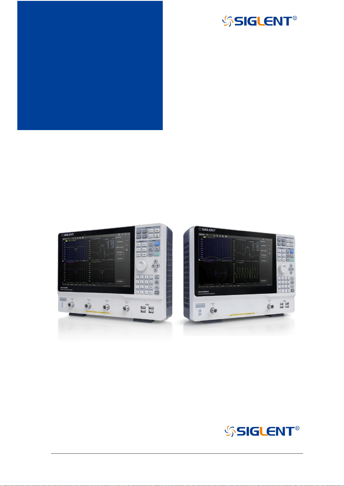
SNA5000A Series
Vector Network
Analyzer
UserManual UM09050-E01A
SIGLENT TECHNOLOGIES CO., LTD
User Manual UM09050-E01C


1 SNA5000A Vector Network Analyzer User Manual
Copyright
◆ SIGLENT TECHNOLOGIES CO., LTD All Rights Reserved.
◆ SIGLENT is the registered trademark of SIGLENT TECHNOLOGIES CO., LTD.
◆ Information in this publication replaces all previously corresponding material.
◆ SIGLENT reserves the right to modify or change parts of or all the specifications or pricing
policies at the company’s sole decision.
◆ Any method of copying, extracting, or translating the contents of this manual is not allowed
without the permission of SIGLENT.
SNA5000A Vector Network Analyzer User Manual 2
Safety requirement
This section contains information and warnings that must be observed to keep
the instrument operating under the corresponding safety conditions. In addition to
the safety precautions specified in this section, you also have to follow common
safe operating procedures.
Safety terms and symbols
When the following terms or symbols appear on the front panel, rear panel,
or this manual, it indicates particular attention should be paid.
Indicates potential injuries or hazards that may happen.
Indicates electric shock that may happen.
Indicates measurement grounding
Indicates safety grounding.
This is a start/standby switch. Press the switch, the VNA will switch between the working state
and the standby state. The switch could not power off the device, to completely power off the
VNA, the power cord must be removed from the AC socket.
Indicates “AC”.
CAUTION
Indicates potential damages to the instrument or other property that may happen.
WARNING
Indicates potential injuries or hazards that may happen.
Operating environment
Use in a clean and dry indoor environment with an ambient temperature range
from 0°C to 40°C.
Note: Direct sunlight, electric heaters, and other direct heat sources, should
be considered when evaluating the ambient temperature.
WARNING: Do not operate the VNA in an explosive, dusty or humid environment.
This instrument meets the EN 61010-1 standard, and has the following
restrictions:
Installation (overvoltage) category: Class II (electric supply connector) and
Class I (measure terminal)
Pollution level: Class II
3 SNA5000A Vector Network Analyzer User Manual
Protection level: Class I
Note:
Installation (overvoltage) category Class II indicates the local supply level is
suitable for equipment connected to the AC power supply.
Installation (overvoltage) category Class I indicates the signal levels suitable
for terminals connected to the RF source.
Pollution level Class II indicates it only occurs in a dry and non-conductive
environment, sometimes we should consider the temporary conductivity caused
by concentration.
Protection level Class I indicates grounding equipment, it prevents electric
shock by connecting the equipment to the ground wire.
CAUTION: Do not apply excessive pressure or strike the surface of the touch screen.
CAUTION: Do not exceed the maximum voltage marked on the front panel connectors.
Cooling requirement
This instrument is cooled through a built-in fan. To keep adequate ventilation,
a gap of at least 15 cm should be left on both sides, as well as the front and rear
panels of the instrument.
CAUTION: Do not block the vents located along the side and real panel of the instrument.
CAUTION: Do not let any external objects enter the instrument through the vents.
AC power supply
The instrument accepts 100-240V, 50/60/400Hz AC power. The maximum
power consumption is 90W with complete options.
Note: The instrument can operate within the following input ranges:
Voltage range:
90 - 264 Vrms
90 - 132 Vrms
Frequency range:
47 - 63 Hz
380 - 420 Hz
Power supply and grounding
The instrument has a three-terminal plug and an IEC320 (Type C13)
standard connector for the input power and grounding connections. The
grounding terminal on the socket is directly connected to the instrument shell. To
prevent electric shock, the plug must be inserted into a well-grounded socket.
Please use the power cord provided to connect the instrument to the power
source.
SNA5000A Vector Network Analyzer User Manual 4
WARNING: Danger of electric shock!
Disconnected or broken internal or external grounding wires will increase the risk of electric shock. It is
strictly forbidden to destroy the protective grounding wire or safety grounding terminals.
The location of the instrument should be convenient to access the power
supply. To completely power off the instrument, the power cord should be
removed from the power socket of the instrument. When the instrument is idle for
long durations, it is recommended to unplug the power cord from the AC socket.
CAUTION: The RF connector’s shell on the front panel is connected to the instrument’s shell, and then
connected to the earth ground.
Calibration
The recommended calibration cycle is one year. Calibration should only be
performed by qualified personnel.
Cleaning
Only a soft damp cloth without any chemical/corrosive substances can be
used to clean the instrument. Do not clean or use the product in wet
environments. To avoid electric shock, unplug the power cord from the AC socket
before cleaning.
WARNING: Danger of electric shock!
Do not disassemble the instrument. Maintenance must be carried out by qualified personnel only.
Exceptional conditions
Use the instrument only for the purpose specified by the manufacturer. Do
not use if the instrument has visible damage or has endured severe
transportation vibration. If the device is suspected to be damaged, please
disconnect the power cord and contact your local SIGLENT office. To operate the
instrument correctly, all instructions and marks should be read carefully.
WARNING: Use of the instrument for purposes unspecified by the manufacturer may damage the
instrument.

5 SNA5000A Vector Network Analyzer User Manual
Product introduction
General Description
The SIGLENT SNA5000A series of vector network analyzers have a frequency range of
9 kHz to 8.5 GHz, which support 2/4-port scattering, differential, and time-domain parameter
measurements. The SNA5000A series are ideal for determining the Q-factor, bandwidth, and
insertion loss of a filter. They feature impedance conversion, movement of measurement
plane, limit testing, ripple test, fixture simulation, and adapter removal/insertion adjustments.
The VNAs have five sweep types: Linear-Frequency mode, Log-Frequency mode, Power-
Sweep mode, CW-Time mode, and Segment-Sweep mode. They also support scattering-
parameter correction of SOLT, SOLR, TRL, Response, and Enhanced Response for
increased flexibility in R&D and manufacturing applications.
Features
◆ Frequency range: 9 kHz-8.5 GHz
◆ Ports: 2/4
◆ Frequency resolution: 1 Hz
◆ Level resolution: 0.05 dB
◆ Range of IFBW: 10 Hz-3 MHz
◆ Setting range of output level: -55 dBm ~ +10 dBm
◆ Dynamic range: 125 dB
◆ Trace noise: 0.003 dBrms , 0.05 °rms
◆ Types of calibration: Response calibration, Enhanced Response calibration, Full-
one port calibration, Full-two port calibration, Full-three port
calibration, Full-four port calibration, TRL calibration
◆ Types of measurement: Scattering-parameter measurement, differential-
parameter measurement, receiver measurement, time-domain
parameter analysis, limit test, ripple test, impedance conversion,
fixture simulation, adapter removal/insertion
◆ Optional Bias-Tees
◆ Interface: LAN, USB Device, USB Host (USB-GPIB)
◆ Remote control: SCPI/Labview/IVI based on USB-TMC/VXI-11/Socket/Telnet/
Webserver
◆ 12.1-inch touch screen
◆ Video output: HDMI

SNA5000A Vector Network Analyzer User Manual 6
User Manual overview
Main Contents
Chapter 1 Quickstart
This chapter introduces the appearance and size of the vector network analyzer, the basic
operation of the front and rear panels, user interface, buttons, and touch screen.
Chapter 2 Basic measurement
This chapter describes the measurement function, sweeping trigger setting, and other
functions of the vector network analyzer, and introduces the functions under each menu in
detail.
Chapter 3 Measurement calibration
This chapter introduces the different calibration methods of S parameters, power calibration
methods, test fixture, and other functions of vector network analyzer in detail.
Chapter 4 Data analysis
This chapter introduces the mathematical analysis function, including time-domain analysis,
windows, coupling, markers, and other functions.
Chapter 5 Guide For TDR Option
This chapter introduces how to use the TDR option.
Chapter 6 Save and recall
This chapter introduces the data save and recall processes.
Chapter 7 System setting
This chapter provides information about the system settings.
Chapter 8 Service and support
This chapter provides information about service and support.

7 SNA5000A Vector Network Analyzer User Manual
Contents
Copyright .................................................................................................................................... 1
Safety requirement .................................................................................................................... 2
Product introduction ................................................................................................................... 5
User Manual overview ............................................................................................................... 6
Contents ..................................................................................................................................... 7
1 Quickstart.......................................................................................................................... 11
1.1 Dimensions ........................................................................................................ 11
1.2 Power supply ...................................................................................................... 11
1.3 Front panel ......................................................................................................... 12
1.3.1 Functional keyboard ................................................................................... 13
1.3.2 Digital keyboard .......................................................................................... 14
1.3.3 Power switch ............................................................................................... 14
1.3.4 RF connectors ............................................................................................ 15
1.4 Rear panel .......................................................................................................... 15
1.5 OCXO option installation guide .......................................................................... 17
1.6 User interface ..................................................................................................... 18
1.6.1 Active entry ................................................................................................. 18
1.6.2 Value of marker ........................................................................................... 19
1.6.3 Trace State ................................................................................................. 19
1.6.4 Channel State ............................................................................................. 19
1.6.5 Function Keys ............................................................................................. 19
1.6.6 Label Page .................................................................................................. 20
1.6.7 Window State .............................................................................................. 20
1.6.8 Stimulus Range .......................................................................................... 20
1.6.9 Status Bar ................................................................................................... 20
1.6.10 Message Bar ............................................................................................... 21
1.6.11 Graffiti Function .......................................................................................... 21
1.7 Touch Screen ..................................................................................................... 24
1.8 Help Information ................................................................................................. 24
2 Basic measurement .......................................................................................................... 25
2.1 Measurement parameters .................................................................................. 25
2.1.1 S parameters .............................................................................................. 25
2.1.2 Balanced S parameters .............................................................................. 25
2.1.3 Power measurement of receiver ................................................................ 26
2.2 Frequency range ................................................................................................ 27
2.2.1 Set the frequency range ............................................................................. 27
2.2.2 CW time sweep or power sweep ................................................................ 27
2.2.3 Frequency resolution .................................................................................. 28
2.3 Power level ......................................................................................................... 28
2.4 Sweep ................................................................................................................ 30

SNA5000A Vector Network Analyzer User Manual 8
2.4.1 Points .......................................................................................................... 30
2.4.2 Sweep type ................................................................................................. 31
2.5 Trigger ................................................................................................................ 33
2.5.1 Trigger Settings ........................................................................................... 33
2.5.2 Trigger source ............................................................................................. 34
2.5.3 Trigger Range ............................................................................................. 34
2.5.4 Channel Settings ........................................................................................ 34
2.5.5 Trigger mode ............................................................................................... 35
2.5.6 External and auxiliary triggers .................................................................... 36
2.6 Data format ........................................................................................................ 40
2.6.1 Display format ............................................................................................. 40
2.6.2 LF Cartesian coordinates display format .................................................... 40
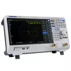
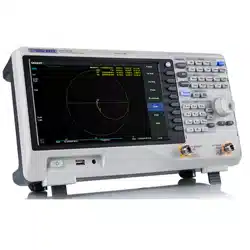
2.6.3 Polar coordinates ........................................................................................ 41
2.6.4 Smith circle diagram ................................................................................... 42
2.7 Scale .................................................................................................................. 44
2.7.1 Scale/reference level and position ............................................................. 44
2.7.2 Scaling coupling .......................................................................................... 45
2.7.3 Electrical delay ............................................................................................ 46
2.7.4 Amplitude offset and amplitude slope ........................................................ 47
2.7.5 Phase deviation .......................................................................................... 47
2.8 Avg BW .............................................................................................................. 48
2.8.1 Overview ..................................................................................................... 48
2.8.2 Averaging .................................................................................................... 48
2.8.3 IF Bandwidth ............................................................................................... 49
2.8.4 Smoothing ................................................................................................... 50
2.9 Preset instructions ............................................................................................. 51
3 Measurement calibration .................................................................................................. 52
3.1 Overview ............................................................................................................ 52
3.2 Calibration type .................................................................................................. 53
3.3 S parameter calibration ...................................................................................... 56
3.3.1 S parameter calibration Kit management ................................................... 56
3.3.2 S Parameter calibration wizard................................................................... 67
3.3.3 Open Response Calibration ....................................................................... 69
3.3.4 Short circuit response calibration ............................................................... 70
3.3.5 Full 1 port OSL calibration .......................................................................... 70
3.3.6 Transmission response calibration (two ports) ........................................... 71
3.3.7 Enhanced response calibration (two ports) ................................................ 72
3.3.8 SOLT calibration (two ports) ....................................................................... 72
3.3.9 SOLR unknown through calibration (two ports) ......................................... 73
3.3.10 TRL Direct Reflection Transmission Line Calibration (Two Ports) ............. 74
3.4 Internal source power calibration ....................................................................... 75
3.5 Receiver calibration ........................................................................................... 77
3.6 Port extension .................................................................................................... 78
3.7 Fixture measurement function ........................................................................... 81
3.8 Adapter removal / insertion function .................................................................. 86
3.9 Ecal .................................................................................................................... 88

9 SNA5000A Vector Network Analyzer User Manual
3.9.1 ECal Overview ............................................................................................ 88
3.9.2 ECal Config ................................................................................................. 89
3.9.3 Confidence Check ...................................................................................... 90
3.9.4 Orientation .................................................................................................. 91
3.9.5 Characterization .......................................................................................... 92
4 Data analysis .................................................................................................................... 93
4.1 Marker ................................................................................................................ 93
4.2 Mathematical operation.................................................................................... 100
4.3 Conversion ....................................................................................................... 101
4.4 Equation editor ................................................................................................. 102
4.5 Trace statistics ................................................................................................. 109
4.6 Limit test ........................................................................................................... 110
4.7 Ripple limit test ................................................................................................. 112
4.8 Bandwidth limit test .......................................................................................... 113
4.9 Time domain .................................................................................................... 114
4.9.1 Transform .................................................................................................. 114
4.9.2 Gating ....................................................................................................... 116
4.9.3 Window ..................................................................................................... 117
4.9.4 Coupling .................................................................................................... 118
4.9.5 Marker ....................................................................................................... 120
5 Guide For The TDR Option ............................................................................................ 121
5.1 Overview .......................................................................................................... 121
5.2 Open/Close/Preset TDR Option ...................................................................... 122
5.3 TDR Setup Wizard ........................................................................................... 122
5.4 Calibration for TDR Option............................................................................... 122
5.4.1 Deskew ..................................................................................................... 122
5.4.2 Deskew & Loss Compensation ................................................................ 123
5.5 TDR Channel Setup ......................................................................................... 124
5.5.1 DUT Topology ........................................................................................... 124
5.5.2 DUT Length ............................................................................................... 124
5.5.3 Stimulus Magnitude in Time Domain ........................................................ 124
5.5.4 Port Impedance ........................................................................................ 125
5.5.5 Velocity Factor & Dielectric Constant ....................................................... 125
5.5.6 Power Level .............................................................................................. 125
5.5.7 Average ..................................................................................................... 125
5.5.8 IF Bandwidth ............................................................................................. 125
5.5.9 Trigger Mode ............................................................................................. 125
5.6 TDR Trace Setup ............................................................................................. 126
5.6.1 Select a Trace ........................................................................................... 126
5.6.2 Scale Management ................................................................................... 126
5.6.3 Memory Trace Management ..................................................................... 127
5.6.4 Measure Parameter & Format .................................................................. 127
5.6.5 Stimulus in Time Domain .......................................................................... 128
5.6.6 Smoothing ................................................................................................. 128
5.6.7 Trace Allocation ........................................................................................ 128

SNA5000A Vector Network Analyzer User Manual 10
5.6.8 Trace Setup Coupling ............................................................................... 129
5.6.9 Time Domain Gating ................................................................................. 129
5.7 TDR Data Analysis & Output ........................................................................... 129
5.7.1 Marker Setup ............................................................................................ 129
5.7.2 Rise Time Search ..................................................................................... 130
5.7.3 Delta Time Search .................................................................................... 130
5.7.4 Peeling ...................................................................................................... 130
5.7.5 File & Data Output .................................................................................... 131
5.8 Eye Diagram Simulation .................................................................................. 131
5.8.1 Overview ................................................................................................... 131
5.8.2 Stimulus Bit Pattern .................................................................................. 131
5.8.3 Stimulus Signal Setup .............................................................................. 133
5.8.4 Eye Diagram Analysis ............................................................................... 133
5.8.5 Eye Diagram Scale Management ............................................................. 134
5.8.6 Mask Test for Eye Diagram ...................................................................... 134
5.8.7 Jitter & Statistical Eye Diagram ................................................................ 134
5.9 TDR Advanced Waveform Function ................................................................ 135
5.9.1 Viewpoint .................................................................................................. 135
5.9.2 Emphasis/De-emphasis ............................................................................ 136
5.9.3 Equalization .............................................................................................. 136
6 Guide For The SA Option ............................................................................................... 136
6.1 Overview .......................................................................................................... 136
6.2 Create a Spectrum Analysis Channel .............................................................. 137
6.3 Spectrum Analyzer Settings ............................................................................. 138
6.3.1 Basic Setup ............................................................................................... 138
6.3.2 Processing setup ...................................................................................... 141
6.4 Other features .................................................................................................. 144
6.4.1 Band Power .............................................................................................. 144
6.4.2 Band Noise ............................................................................................... 145
6.4.3 Occupied BW ............................................................................................ 146
7 Save and recall ............................................................................................................... 147
8 System setting ................................................................................................................ 149
9 Service and support........................................................................................................ 155
9.1 Ordering and activating the options ................................................................. 155
9.2 Warranty overview ........................................................................................... 156
11 SNA5000A Vector Network Analyzer User Manual
1 Quickstart
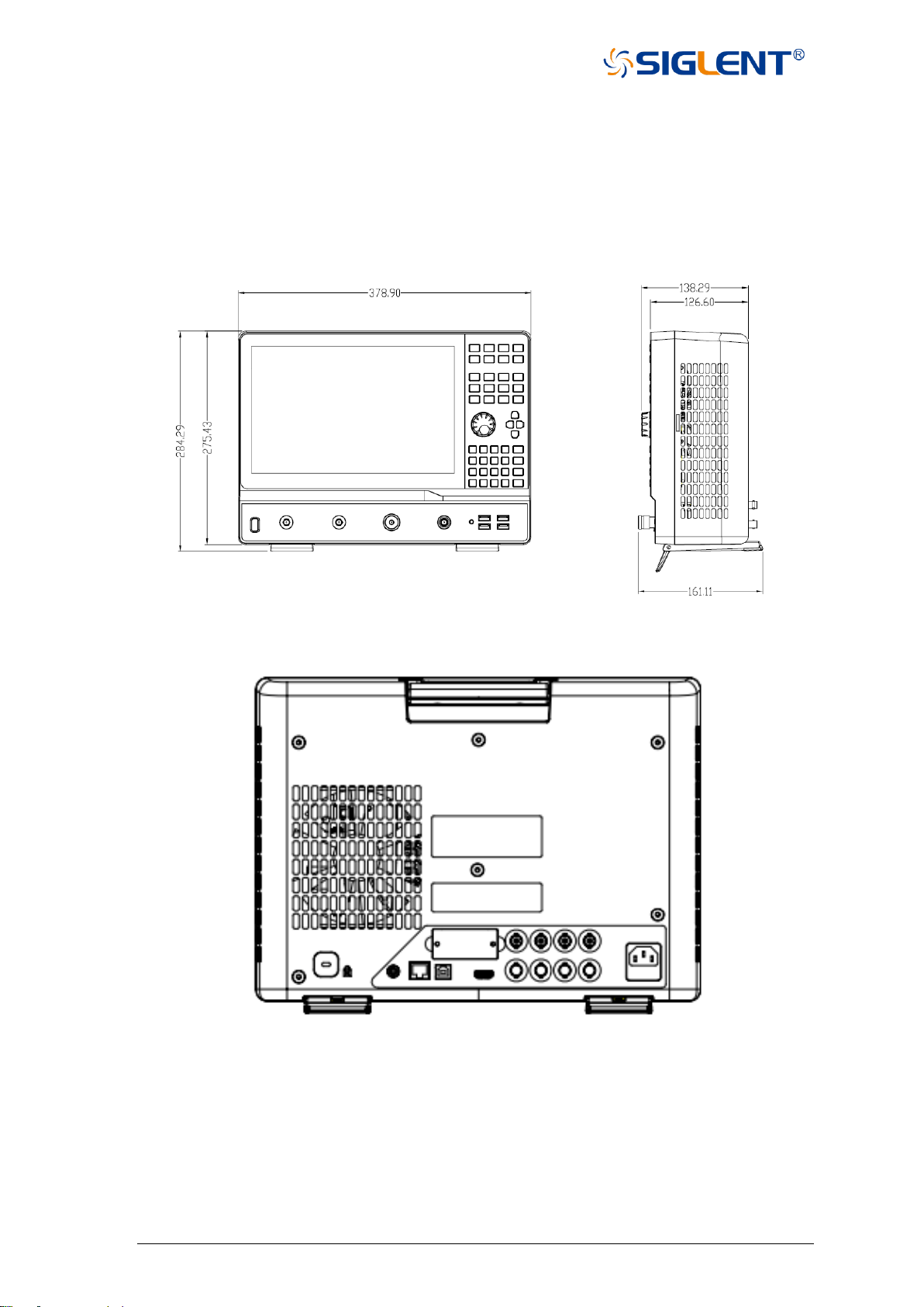
1.1 Dimensions
Figure 1-1 Front view and side view
Figure 1-2 Rear panel view
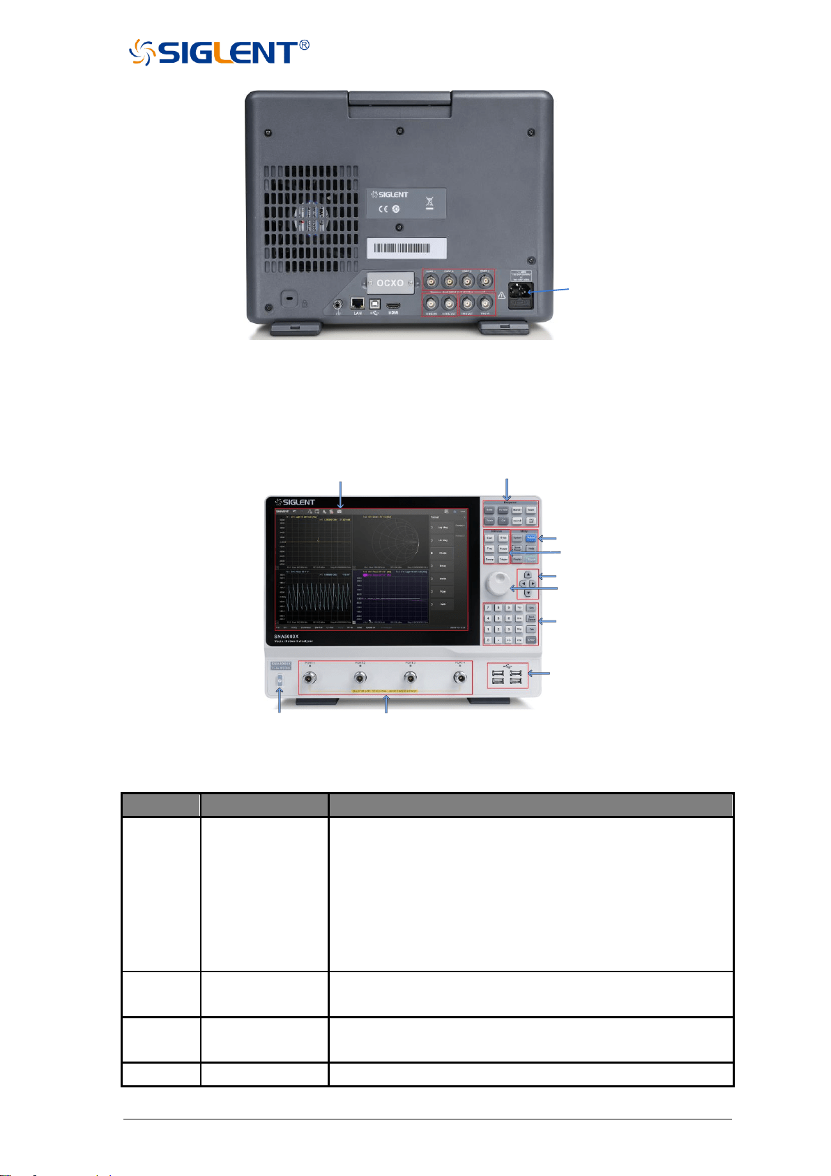
1.2 Power supply
The equipment accepts 100-240V, 50/60/400Hz AC power supplies. Please use the power
cord provided to connect the instrument to the power source as shown in the figure below.
SNA5000A Vector Network Analyzer User Manual 12
Power
Interface
Figure 1-3 Power interface
1.3 Front panel
LCD Touchscreen
Response
Utility
Stimulus
Navigation
Knob
Numeric
USB Hub
Test Ports
Power Switch
Figure 1-4 Front panel
Table 1-1 Front panel area description:
Number
Items
Description
1
LCD
Touchscreen
12.1 inch TFT color capacitive LCD touchscreen.
Notes: Avoid touching the LCD touchscreen with
sharp objects. The effective pixel ratio of the screen is more
than 99.998%, so it doesn't mean a fault when the screen
has some black/blue/green/red fixed points less than
0.002%. Screen savers are not recommended. The LCD
screen is unlikely to suffer from image burn-in.
2
Response
Includes the setting of measurement parameters, parameter
format, markers, calibration, and so on.
3
Utility
Includes the function keys of the system, help, display, and
so on.
4
Stimulus
Includes the setting of measurement frequency, sweep time,
13 SNA5000A Vector Network Analyzer User Manual
sweep points, trigger, and so on.
5
Navigation
Press the up, down, left, and right buttons to select the
desired operation.
6
Knob
Rotate the button left or right to move the cursor or change
the parameter value, the effect of pressing the button is the
same as ”Enter”.
7
Numeric
Includes the parameter numbers and units.
8
USB Hub
Includes four USB ports for data exchange and power
supply with peripherals. The total current of four USB ports
is less than 2A.
9
Test ports
Connect to the DUT for signal transmission and reception.
10
Power Switch
Power on/off the equipment.
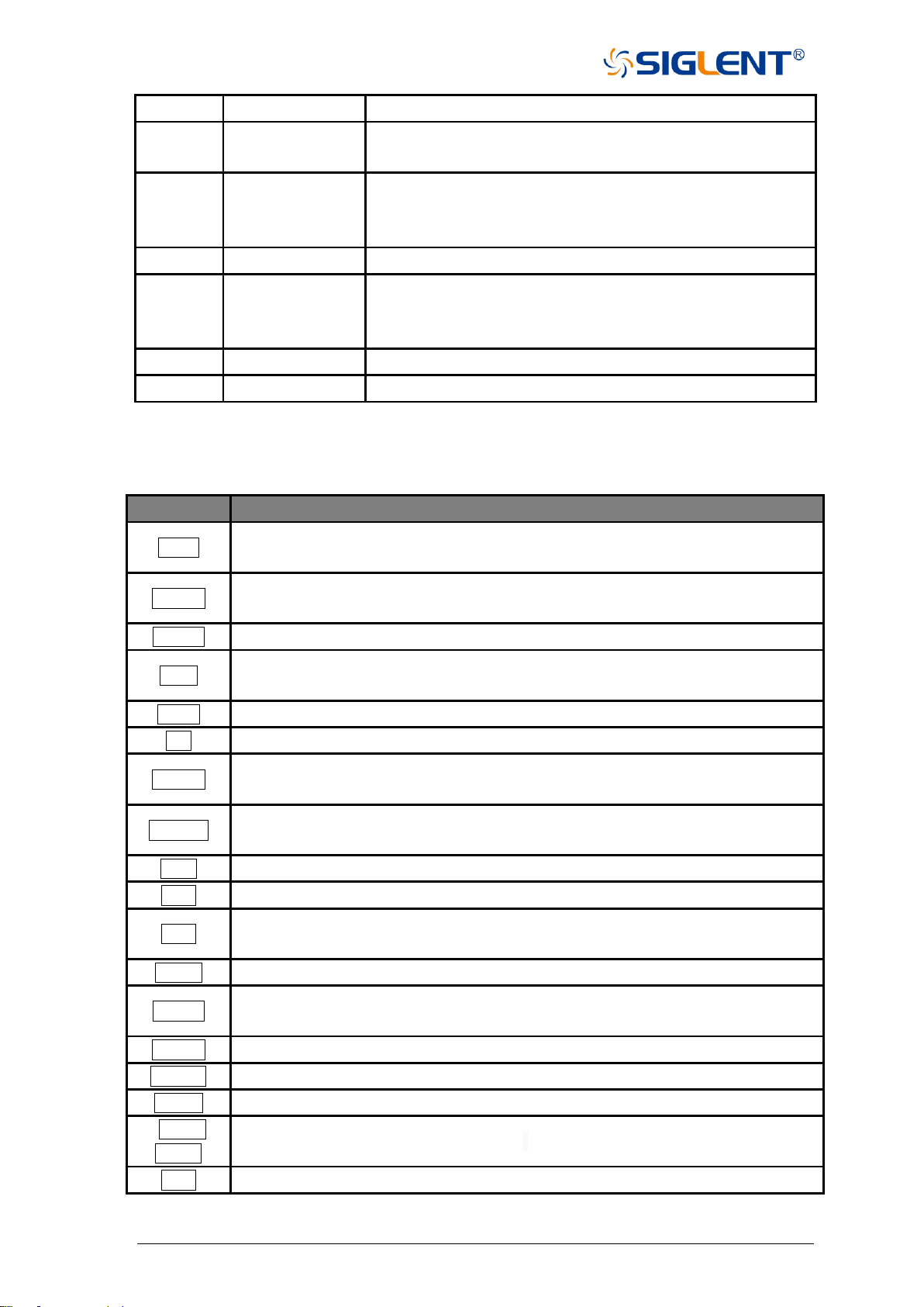
1.3.1 Functional keyboard
Table 1-1 Front panel functional keyboard description:
Keys
Description
Meas
Set the single-ended/ differential S parameter measurement, reference/
measurement receivers power measurement, and so on.
Format
Set the measurement parameter’s display format, such as Log Mag, Lin Mag,
Smith Chart, Polar Chart, SWR, Phase, and so on.
Marker
Set markers to obtain the value of measurement parameters.
Math
Contains storing measurement data in memory, comparing current data with
previous data, time-domain analysis of measurement results, and so on.
Scale
Set the scale of parameter levels.
Cal
Include the setting of S parameter calibration and power calibration.
Search
Press this button to get the measurement parameter’s maximum/minimum
value, bandwidth, Q-factor, and so on.
Avg BW
Press this button to smooth/average measurement data, set the receiver’s IF
bandwidth, and so on.
Start
Set start frequency.
Stop
Set stop frequency.
Freq
Set start frequency, stop frequency, center frequency, frequency span,
measurement point.
Power
Set the RF power level, turn on/off RF power, and so on.
Sweep
Set sweep mode, sweep point, sweep time, log/lin frequency sweep mode, and
so on.
Trigger
Press this button to choose the trigger source, set the trigger mode, and so on.
System
Set IP address, system time, language, and so on.
Preset
Press this button to revert to the default parameters.
Save
Recall
Save and recall the measurement data, status, calibration data.
Help
Open the help file.
SNA5000A Vector Network Analyzer User Manual 14
Display
Set measurement window, measurement channel, measurement trace, and so
on.
Touch
Press this button to turn on/off the screen’s touch function.
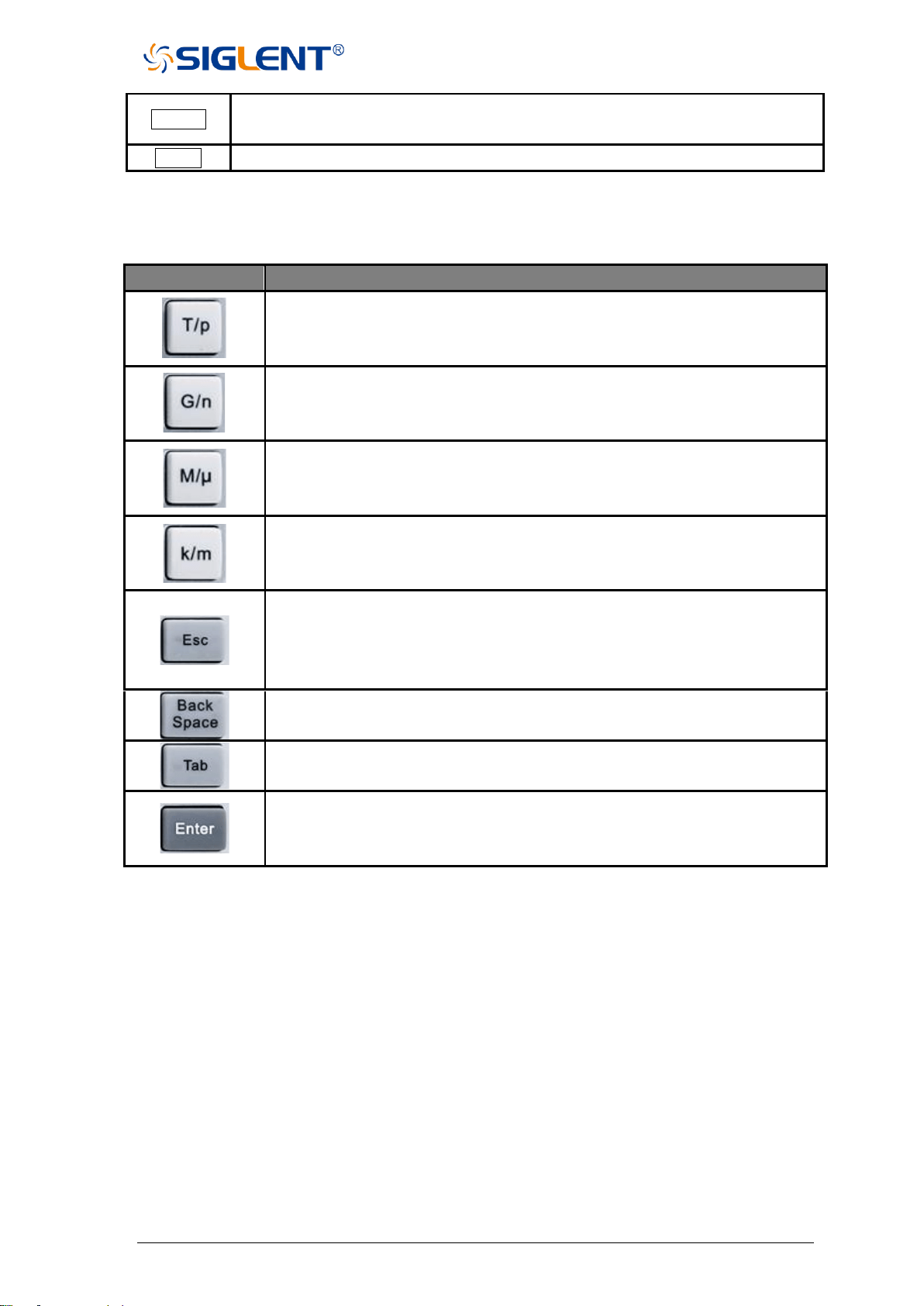
1.3.2 Digital keyboard
Table 1-3 Front panel digital keyboard description:
Keys
Description
When setting the frequency, press this key to set the unit as THz. if the input
is time-related, press this key to set the unit as ps.
When setting the frequency, press this key to set the unit as GHz. if the input
is time-related, press this key to set the unit as ns.
When setting the frequency, press this key to set the unit as MHz. if the input
is time-related, press this key to set the unit as us.
When setting the frequency, press this key to set the unit as kHz. if the input
is time-related, press this key to set the unit as ms.
During the parameter editing process, pressing this button will clear the input
of the active function area and exit the parameter input state. Press this
button to return to local control if previously controlling the instrument
remotely.
During the parameter editing process, pressing this button will clear the input
of the active function area from right to left.
Pressing this button will activate every sub-function area from top to bottom
in turn.
In the parameter input process, pressing this button will end the parameter
input process and add the currently set units for the parameter.
1.3.3 Power switch
Stand-by is indicated by a constant orange-colored power switch.
A single button press will cause the light to turn white which indicates the instrument is
operating.
Continuous white indicates the instrument is operating.
A short press of this button (one second) causes the light to turn orange which indicates
the instrument is in the stand-by state after saving the settings.
A long press of this button (three seconds) will cause the light to turn orange which
indicates the instrument is in the stand-by state immediately without saving the settings.
15 SNA5000A Vector Network Analyzer User Manual
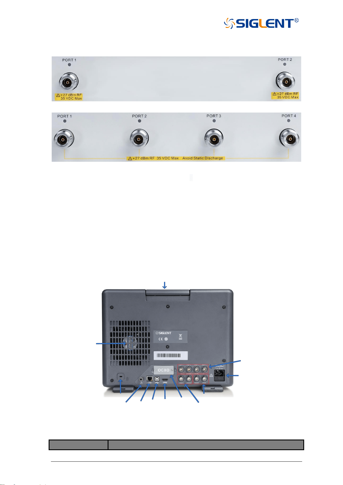
1.3.4 RF connectors
Figure 1-5 Front panel RF connectors (2-port VNA)
Figure 1-6 Front panel RF connectors (4-port VNA)
◆ The number of RF connectors is two or four, depending on the instrument
configuration.
◆ When an RF connector is transmitting an RF signal, the corresponding orange light
above the RF connector will be lit.
◆ To avoid damage to the instrument, the RF connector input signal must meet the
following: The DC voltage and the maximum continuous RF power cannot exceed 35
V and 27 dBm respectively.
1.4 Rear panel
Ground
Terminal
LAN
Port
USB
Port
HDMI
Port
OCXO
Ref In/Out
Trig In/Out
Lock
AC Power
Port and Fuse
Bias-Tees
Ports
Fan
Handle
Figure 1-7 Rear panel
Table 1-4 Rear panel area description:
Items
Description

SNA5000A Vector Network Analyzer User Manual 16
Handle
Portable handle to carry the instrument.
Fan
Used to cool down internal components of the instrument.
Lock
Used to fix the instrument on the fixed object such as a table to help
prevent theft.
Ground Terminal
Connect the instrument with earth ground. Electrically connects the
metallic shell and connectors of the instrument to earth ground.
LAN Port
Used to connect the instrument to a LAN for data exchange with
peripherals such as PCs.
USB Port
Include one USB port for data exchange with peripherals.
HDMI Port
Connect the port to a compatible external monitor.
OCXO
Install the OCXO option to use the high-performance reference source.
10MHz Ref Signal
Input
The characteristic impedance of this port is 50 Ω. The detectable input
frequency and power range are 10 MHz ± 10 ppm, -3 dBm to +10
dBm respectively. When there is a 10 MHz external reference signal
on the port, the VNA’s transmitting signal will be locked into this 10
MHz external reference signal. Otherwise, the VNA’s transmitting
signal will be locked into the internal 10 MHz reference signal.
10MHz Ref Signal
Output
This port can output a 10 MHz reference signal so that it can be used
by other equipment. The characteristic impedance, output frequency,
and power range are 50 Ω, 10 MHz ± 10 ppm,-3 dBm to +10 dBm
respectively.
Trigger In
When there is an external trigger signal at the port, the VNA will use
this external trigger signal instead of the internal trigger signal.
Input level:
Low threshold voltage: 1.1 V
High threshold voltage: 2.5 V
Input level range: 0 to + 5 V
Pulse width:
≥ 2μs
Polarity:
Positive or negative
Trigger Out
This port can output a trigger signal so that it can be used by other
equipment.
Max output current:
20 mA
Output level:
Low-level voltage: 0 V
High-level voltage: 3.3 V
Pulse width:
1μs
Polarity:
Positive or negative
Bias-Tees Ports
Connect an external DC voltage source to this port to provide DC power
for the DUT such as a power amplifier. The DC voltage and current
cannot exceed 35V. This is the rated current of the fuse.
17 SNA5000A Vector Network Analyzer User Manual
AC Power Port and
Fuse
The equipment accepts 100-240 V, 50/60/400 Hz AC power supply.
please connect the VNA to the AC power supply with the supplied power
cord. Make sure the current does not exceed the rated current of the
fuse.
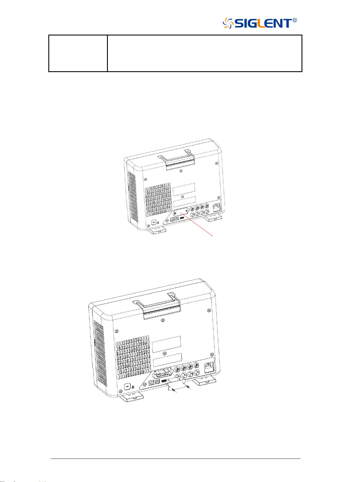
1.5 OCXO option installation guide
◆ Power off the instrument, use a screwdriver to remove the cover where the OCXO option
is located on the rear panel.
Cover
Figure 1-8 OCXO option installation guide
◆ Insert the fixed OCXO module into the instrument’s slot, then tighten the screws.
Figure 1-9 OCXO option installation guide
◆ Power on the instrument and install the OCXO option’s license activation code for
permanent installation.
SNA5000A Vector Network Analyzer User Manual 18
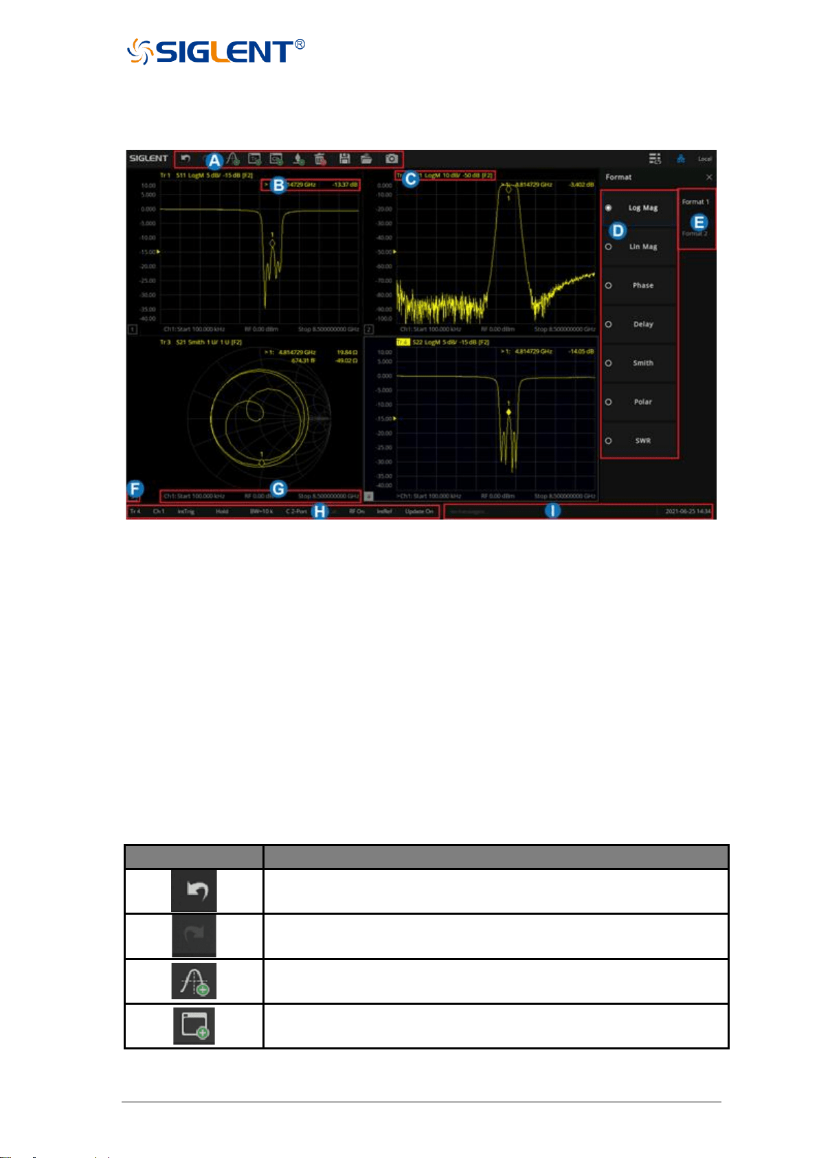
1.6 User interface
Figure 1-10 User interface
A. Active Entry
B. Marker Readout
C. Trace Status
D. SoftKeys
E. Softtabs
F. Window number
G. Stimulus Range
H. Status Bar
I. Message Bar
1.6.1 Active entry
Table 1-5 Active entry description:
Functions
Functions Description
Recall the previous step.
Recovering the withdrawn operation.
Add a measurement trace.
Add a measurement window.
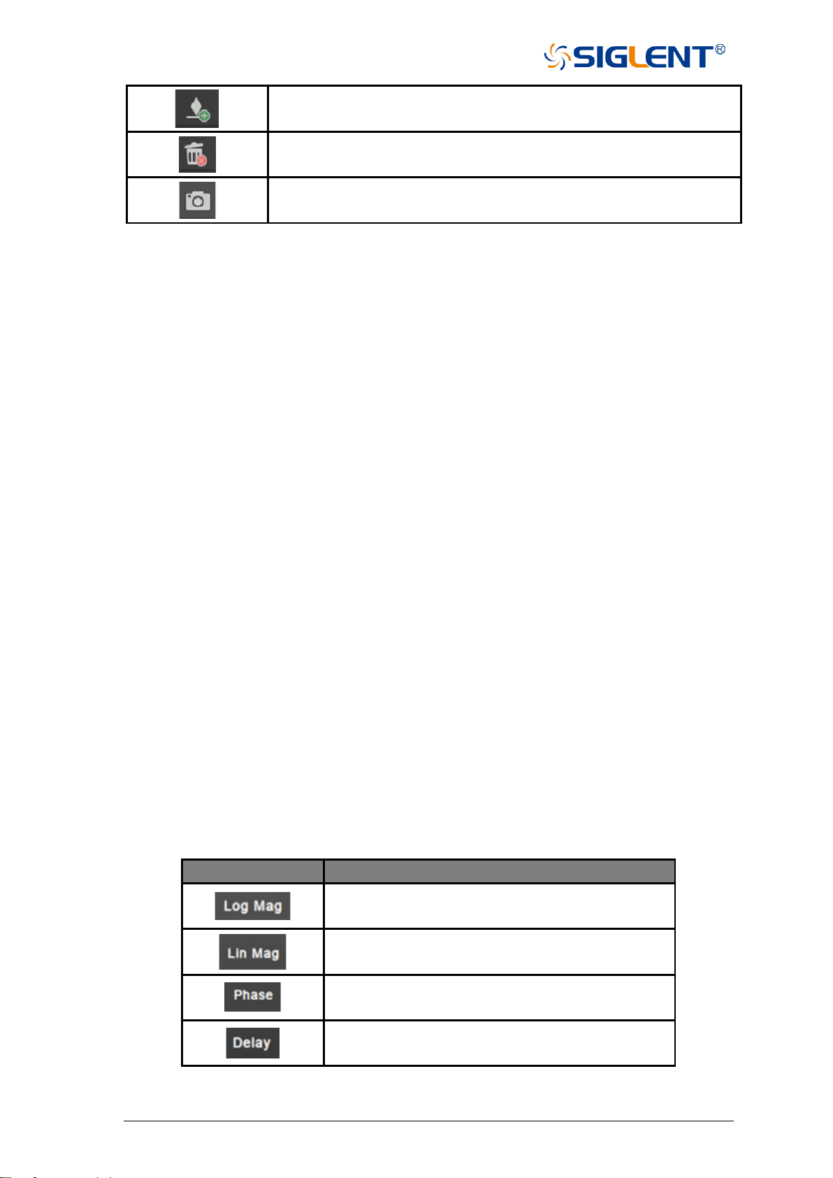
19 SNA5000A Vector Network Analyzer User Manual
Add a marker.
Delete active window or trace.
Note: Keep at least one trace on the interface.
Screenshot (Ctrl+P)
1.6.2 Value of marker
Display the frequency and reading of the marker.
1.6.3 Trace State
◆ A trace is a series of measured data points. Up to 256 traces can be created. In addition,
one historical memory trace for each active trace can be stored and displayed.
Mathematical operations can be performed on the current trace data and the historical
memory trace.
◆ Press the Display button in the front panel, and the Trace Setup menu pops up on the
right side of the screen to manage the operation Trace, such as adding a trace, deleting a
trace, maximizing the trace window, moving traces between Windows, keeping the trace
to the maximum or minimum value without displaying the current value, etc.
◆ Select a trace line and press the Scale button to change the reference electric equalization
operation.
1.6.4 Channel State
◆ Channels contain traces. Up to 256 channels can be created. The channel setting
determines how trace data is measured, and all traces assigned to a channel share the
same channel setting.
◆ Press the Display button in the front panel, and the Channel Setup menu pops up on the
right side of the screen. This can be used to manage operation channels, such as adding
channels, copying channels, and deleting channels.
1.6.5 Function Keys
Table 1-6 Function Keys Interface Description
Functions
Functions Description
Parameters are displayed in logarithmic amplitude
mode.
The parameters are displayed in amplitude linear
fashion.
Displays the phase of the parameter.
Displays the delay of the parameter.
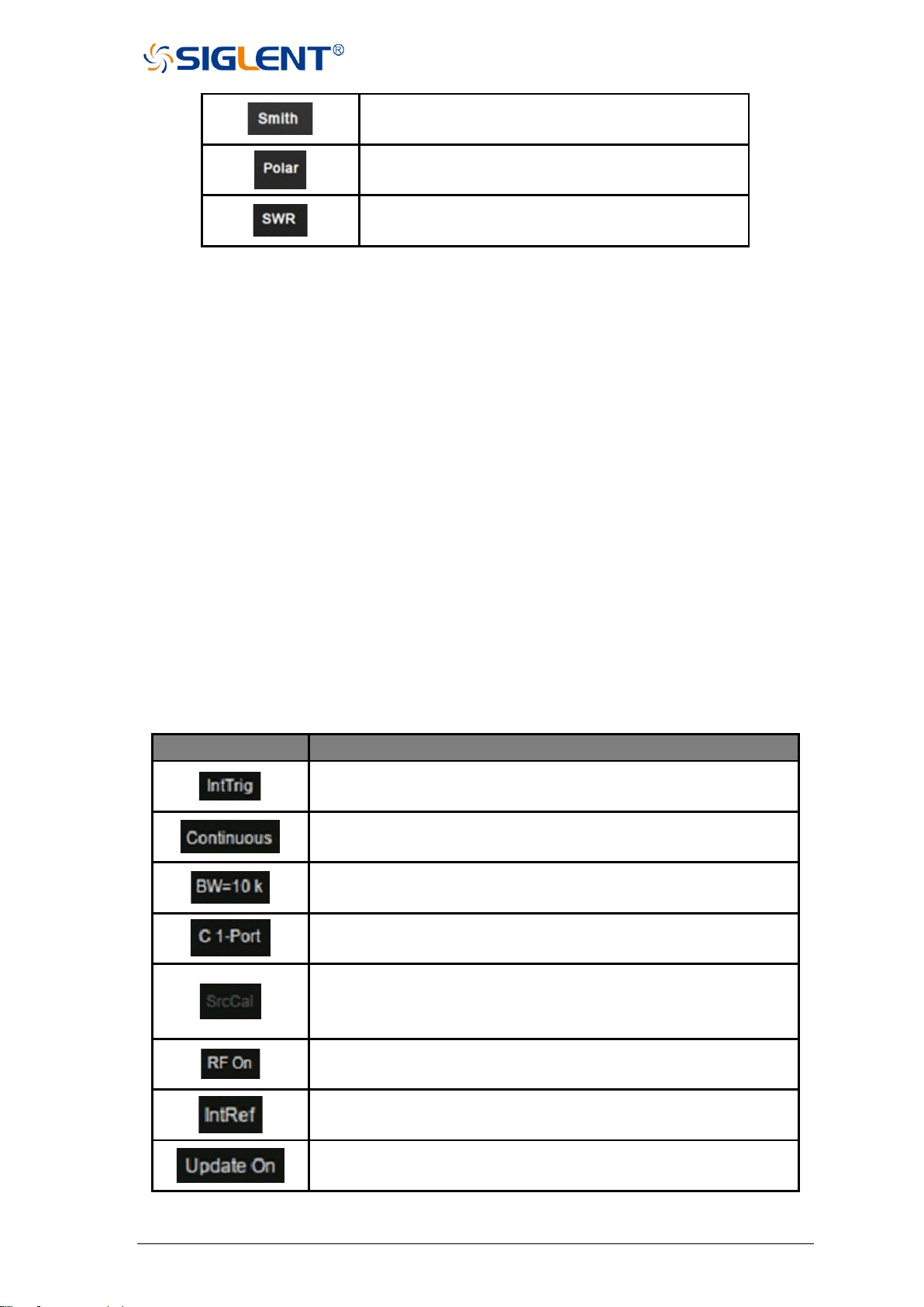
SNA5000A Vector Network Analyzer User Manual 20
The parameters are shown in the form of a Smith
chart.
The parameters are displayed in polar coordinates.
The parameters are shown in SWR.
1.6.6 Label Page
Displays all parameter display formats supported by the vector network analyzer.
1.6.7 Window State
◆ Windows can be used to view trace data and up to 100 windows can be created.
◆ Press the button of Display in the front panel and the Window Setup menu pops up on
the right side of the screen. It can be used to manage operation windows, such as
selecting a window, adding a window, deleting a window, maximizing a window, layout,
and so on.
1.6.8 Stimulus Range
Displays the excitation signal set in the current window, including starting frequency, ending
frequency, internal source output power, etc.
1.6.9 Status Bar
Table 1-7 Status Bar Interface Description
Functions
Functions Description
Displays the current trigger mode.
Continuous trigger, single trigger, and other trigger mode displays.
Display of the current IF bandwidth.
S parameter calibration data state loading display.
Display whether the internal source power calibration data state is
loaded or not. A Gray dark shaded label represents an unavailable
selection/option.
Internal source output power ON and off, RF ON stands for ON.
A display that currently uses an internal or external reference
signal.
UI waveform update or not.
21 SNA5000A Vector Network Analyzer User Manual
1.6.10 Message Bar
Displays the current date information and error information during testing.
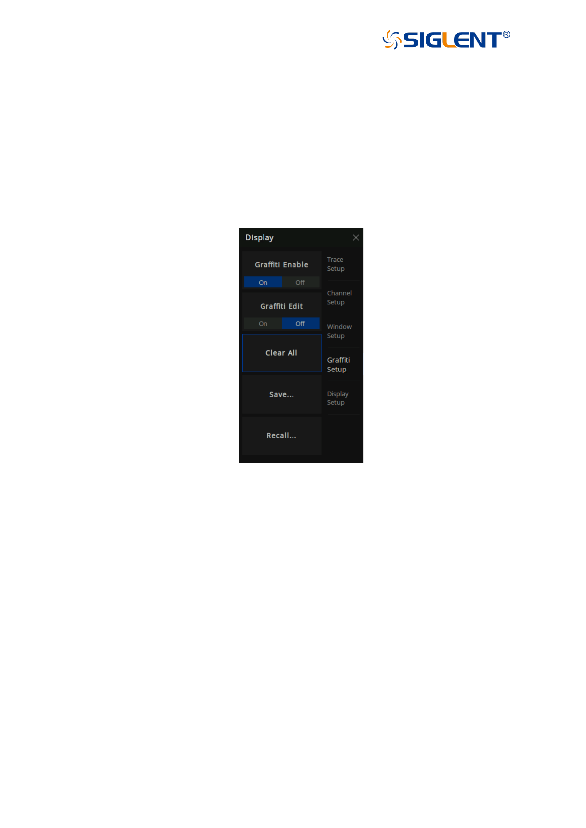
1.6.11 Graffiti Function
This product provides a basic graffiti function, which is used to draw graphics and mark
information on the main interface. This feature is great for annotating screenshots and adding
important details before saving.
⚫ Graffiti function menu bar
Figure 1-11 graffiti function menu bar
As shown in Figure 1-11, the graffiti menu contains functions of enable, edit, clear, save and
call.
⚫ Graffiti Editing Interface
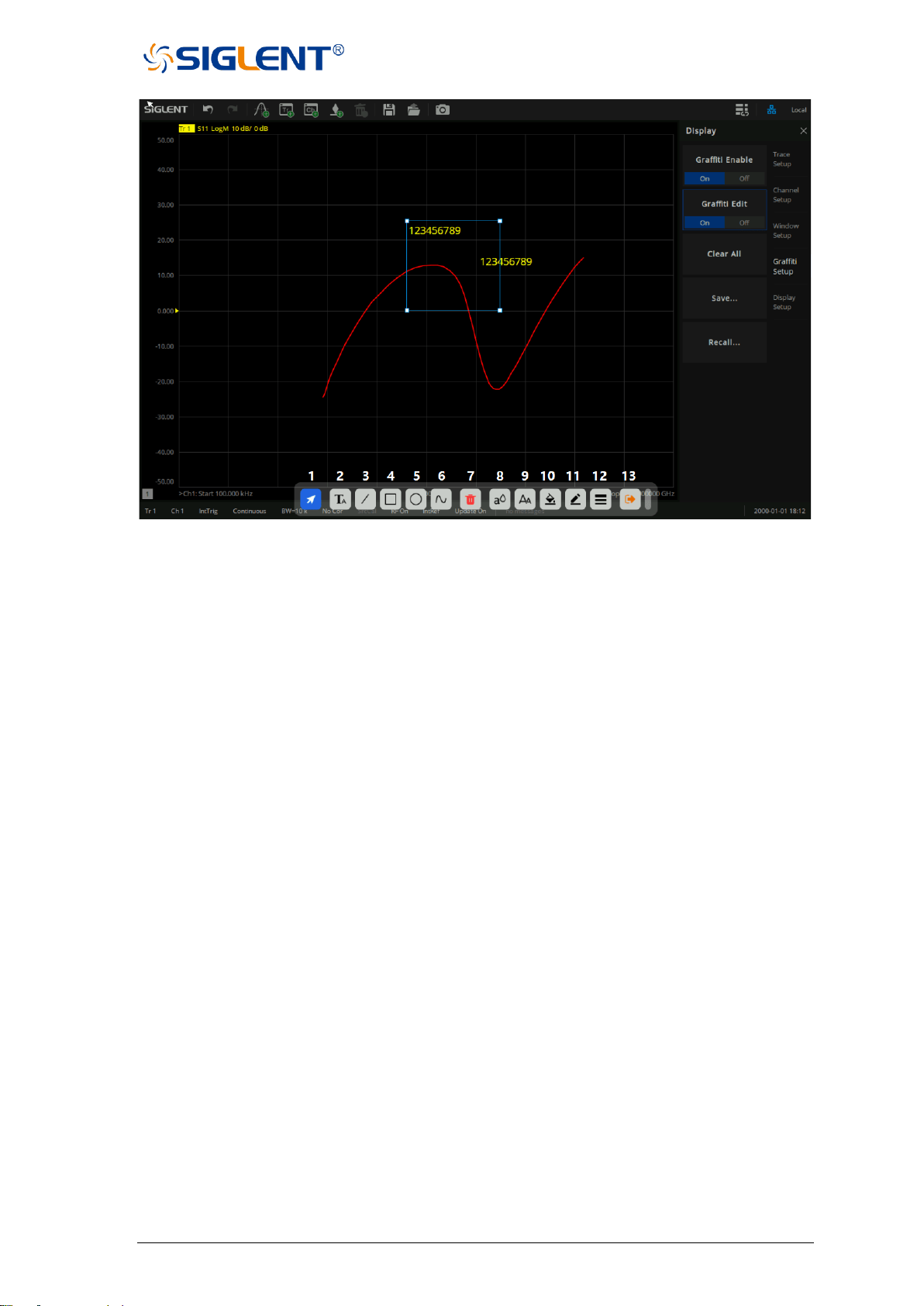
SNA5000A Vector Network Analyzer User Manual 22
Figure 1-12 graffiti editing interface
As shown in Figure 1-12, the toolbar at the bottom of the interface displays a series of tools for
graphic editing:
1. Selection tool: A series of editing can be carried out after the drawing is selected
2. Text tool: Add text notes in the interface
3. Line tool: Add a line in the interface
4. Rectangle tool: Add a rectangle to the interface
5. Ellipse tool: Add an ellipse to the interface
6. Curve tool: Draw a series of lines arbitrarily in the interface (double click the mouse / double
click the finger on the screen to finish drawing)
7. Delete tool: Delete the currently selected drawing
8. Text color tool: Set text color (support graphics: text)
9. Text size tool: Set text size (support graphics: text)
10. Background filling tool: Fill graphics background color (support graphics: text, rectangle,
ellipse)
11. Border color tool: Set the border color of graphics (support graphics: text, line, rectangle,
ellipse, curve)
12. Border line tool: Adjust the border line thickness of graphics (support graphics: text, line
segment, rectangle, ellipse, curve)
13. Exit editing tool: Exit the current editing state
23 SNA5000A Vector Network Analyzer User Manual
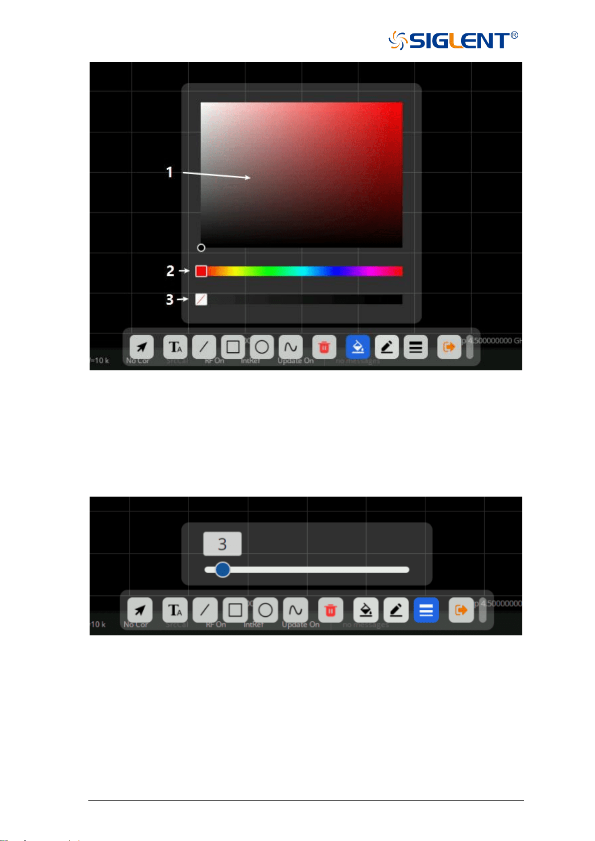
Figure 1-13 Color selection interface
As shown in Figure 1-13, after calling out this interface, you can adjust the corresponding colors
of the graphics:
1. Color shade selection tool: Mouse/finger click to select the appropriate brightness of the
color
2. Color selection tool: Select a specific color
3. Color transparency tool: Adjust color transparency (the more right, the lower color
transparency)
Figure 1-14 Line thickness adjustment interface
As shown in Figure 1-14, you can adjust the line thickness at the edge of the graph by calling
out this interface. The larger the value is, the thicker the line will be.
⚫ Save/Recall
Click the save menu button to save the current graffiti content as a file with *.GFT as the file
extension.

SNA5000A Vector Network Analyzer User Manual 24
1.7 Touch Screen
The vector network analyzer is equipped with a 12.1-inch high-resolution color touch LCD
screen for trace, function keys, and other measurement-related information. With the help of
the touch screen, the LCD screen can be directly touched by a finger to select measurement
and parameter setting operations.
◆ When the Touch button display light is on, the touch screen function is on.
◆ When the Touch button display light is off, the touch screen function is off.
◆ Sliding the screen up and down to display the coordinates of the vertical axis can
continuously change the parameters of the vertical axis.
1.8 Help Information
The Help system of the vector network analyzer can provide the Help information of the
function keys and menu options on the front panel. Press the Help button on the front panel to
enter the Utility menu, click Help to open the Help document, click into the corresponding
directory to view the information.

25 SNA5000A Vector Network Analyzer User Manual
2 Basic measurement
This chapter introduces in detail each function button on the front panel of SNA5000A series
vector network analyzers and the following menu functions.
2.1 Measurement parameters
2.1.1 S parameters
S parameters are used to describe the degree of a transmitted or reflected signal through
an impedance discontinuity. S parameters are relative measurements, defined as the ratio of
two complex voltages. They contain the amplitude and phase information of the relevant
signals. For the 2-port vector network analyzer, there are 4 S parameters (S11, S21, S12, S22).
The specific meaning of each S parameter can be described by the following items:
Sxy x,y∈(1,2):
x:
The response port is also known as the receiving port of the vector network
analyzer. The transmitted signal enters the port after passing through the DUT.
y:
The excitation port is also known as the transmitting port of the vector network
analyzer. The output signal of this port is provided to the DUT.
Here is a list of common S parameter measurements:
Reflection parameters
Transmission parameters
• Return loss
• SWR
• Reflection coefficient
• Input impedance
• S11, S22
• Insertion loss
• Transmission coefficient
• Gain/loss insertion
• group delay
• Linear phase shift
• electrical delay
• S21, S12
2.1.2 Balanced S parameters
Balanced S parameters are also relative. They are used to measure the S parameters of
differential ports such as those found on baluns and transformers. They are also defined as
the ratio of complex voltages, which contain the amplitude and phase information of relevant
signals. The topology and logical port mappings for the differential devices to be tested need
to be created or edited before the test. "Logical ports" are used to describe the test ports of the
physical vector network analyzer that have been remapped to the new port.
1. Map any two physical ports of the vector network analyzer to a balanced logical port.

SNA5000A Vector Network Analyzer User Manual 26
2. Map any physical port of the vector network analyzer to a single-terminal logical
port.
These Settings are applied to "all" measurement trace lines in the channel, and if the
topology of the differential device under test changes, all existing measurements in the channel
that are not compatible with the new topology will automatically change to compatible
measurements.
The following are the topological relationships of several common differential devices. A
multi-port vector network analyzer can be used to measure the following topological
relationships for differential devices. When the vector network analyzer has only 2 test ports,
then only the first balanced device under test can be tested. When the vector network analyzer
has four test ports, then all the devices under test with the following four topological
relationships can be tested.
• Balanced
(1 logical port, 2 actual ports)
• Balanced/balanced
(2 logical ports, 4 actual ports)
• Single-ended/balanced
(2 logical ports, 3 actual ports)
• Single-ended - Single Ended/Balanced
(3 logical ports, 4 actual ports)
2.1.3 Power measurement of receiver
Each port of the vector network analyzer contains 1 reference receiver and 1
measurement reference receiver. For the 4-port vector network analyzer, there are a total of 4
reference receivers and 4 measurement reference receivers. The power measured by these
receivers can be compared to obtain all the S parameter indices.
R1, R2, R3, and R4 are the reference receivers used to measure the signal emitted from
the vector network analyzer, It is equal to the transmitted power at the port after power
calibration.
• R1: Measures the output power of port 1
• R2: Measures the output power of port 2
• R3: Measures the output power of port 3
• R4: Measures the output power of port 4
A, B, C, and D are test receivers used to measure the reflected or transmitted signal
power after passing through the device under test.
• A: Measures the signal power entering port 1
• B: Measures the signal power entering port 2
• C: Measures the signal power entering port 3

27 SNA5000A Vector Network Analyzer User Manual
• D: Measures the signal power entering port 4
2.2 Frequency range
2.2.1 Set the frequency range
Set the range of RF frequencies.
Operating steps:
Press Freq on the front panel to open the frequency setting interface, parameter change
mode:
1. Use the numeric keypad to input the value of the frequency and press the unit button
to select the desired unit. The optional units are GHz, MHz, KHz, and Hz. Press
Enter to select the current unit by default.
2. Press ENTER or the multifunction knob to enter the state of parameter editing. Move
the cursor to the specified position by the left and right arrow keys. Modify the value
by pressing the up and down key, rotating the knob, or pressing the numeric keypad.
Press ENTER, the knob, or ESC to exit the editing mode.
Note:
• Start: Specify the starting frequency of the scanning measurement range
• Stop: Specify the end frequency of the scanning measurement range
• Center: Specify a center frequency value, which can be anywhere in the range of the
vector network analyzer
• Span: Specify the frequency value span measured on either side of the center frequency
• Step: Specify the step size
• Points: Specify the number of measurement points
2.2.2 CW time sweep or power sweep
Measurements using a CW time sweep or power sweep will be performed on a single
frequency rather than the entire frequency range
Operating steps:
Press Sweep, use the knob or arrow keys to focus on the Sweep→Sweep type.
Parameter change mode:
1. Press ENTER or the knob to enter the parameter editing state and then move the
cursor to the specified position by up and down arrow keys or the knob to set the
Sweep type to CW Time or Power Sweep. Press ENTER or the knob to select the
current option.
2. Press Freq, use the knob or arrow keys to focus on the Freq→CW parameter entry.
Select the edit box to enter the edit mode and change the value by pressing the up

SNA5000A Vector Network Analyzer User Manual 28
and down key, rotating the knob, or pressing the numeric keypad. Press ENTER, the
knob, or ESC to exit editing mode.
2.2.3 Frequency resolution
Set the frequency resolution to 1Hz.
2.3 Power level
Power level refers to the output power at the port of the vector network analyzer.
Here are the keys to operation:
1. Press Power, use the knob or arrow keys to focus on the Power→Power Level
parameter item. Input the required power level. Press ENTER to exit editing mode. The
default unit is dBm.
2. Press Power, use the knob or arrow keys to focus on the Power→RF Power parameter
item. Turn on or off RF power.
3. Press Power, use the knob or arrow keys to focus on the Port Power parameter item,
Configure start and stop power. Start and stop power are only available in power sweep
mode.
4. Press Power, use the knob or arrow keys to focus on the Port Power→Select
parameter item, Press ENTER or the knob to select the corresponding power port.
5. Press Power, use the knob or arrow keys to focus on the Port Power→Coupling
parameter item, Press ENTER or the knob to choose to turn coupling off or on.
6. Press Power, use the knob or arrow keys to focus on the Leveling & Offsets→Slope
Enable parameter item, Press ENTER or the Knob to turn on the Slope switch, Press
Leveling & Offsets→Slope to set the Slope.
Coupled port power:
• Coupling (selected): The power level of each test port is the same. If the power of any test
port is set, the power of all test ports will change accordingly.
• Decoupling (clearing): Set the power level for each test port separately and decouple the
Power. For example, if you want to measure the gain and reverse
isolation of a high gain amplifier, the input port of the amplifier
requires much less power than the output port. Power sweep can
also be performed using uncoupled power.
Power Leveling&Offsets
29 SNA5000A Vector Network Analyzer User Manual
Power Limits controls the source power at each test port for ALL channels. Use this feature
to protect DUTs that are sensitive to overpowering at the input. Source Power levels that
exceed the Limit at the specified port are clipped at the limit, and an error message is
displayed on the screen.
Power Offset provides a method of compensating port power for added attenuation or
amplification in the source path. The result is that power at the specified port, all dialogs, and
annotations reflect the added components. For amplification use a positive offset, and for
attenuation use a negative offset.
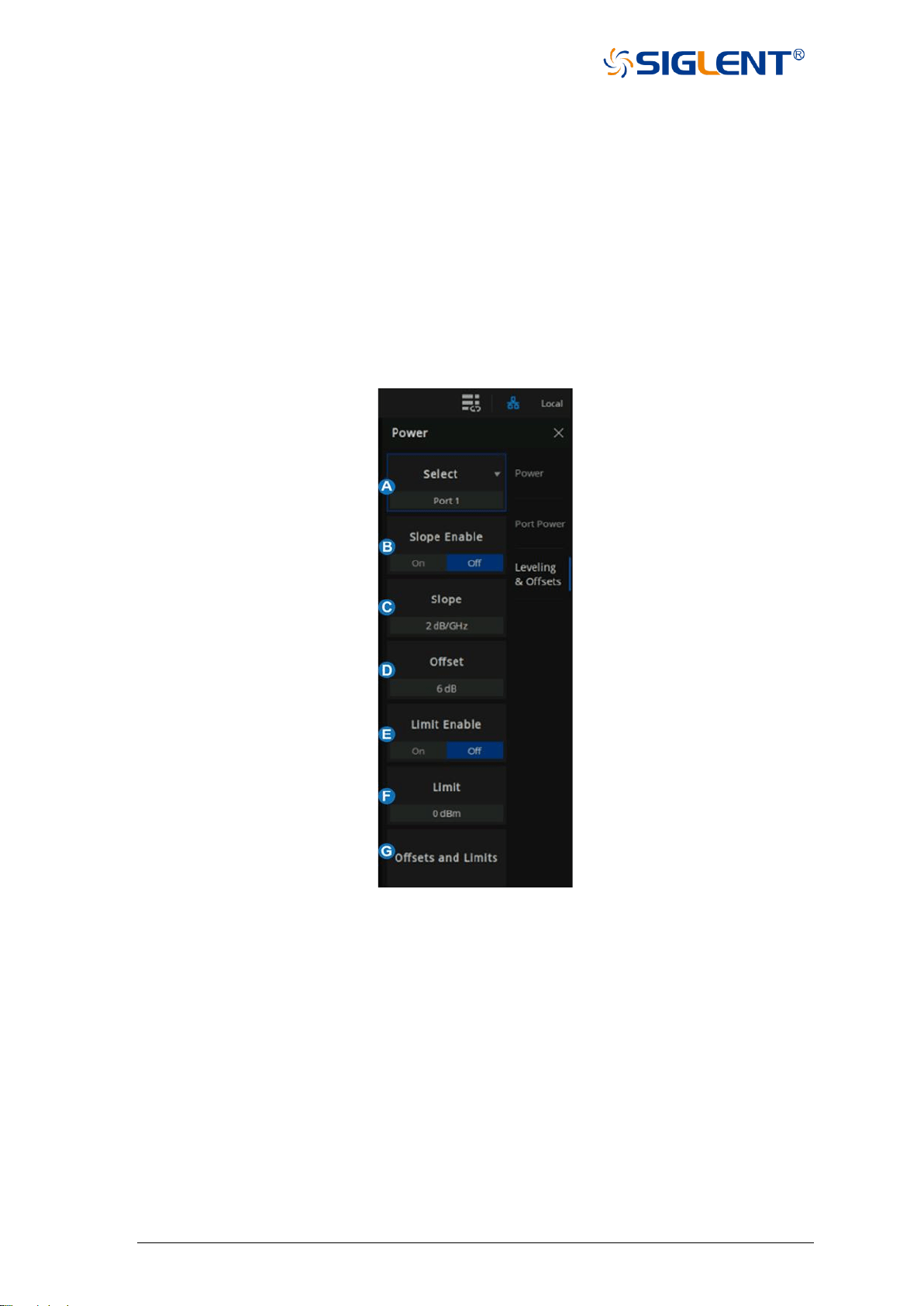
Using the Softkey for setting: Press the ”Power” key, “Power” > Leveling & Offsets then enter
the menu.
A. Select the Port.
B. Slope Enable. Helps compensate for cable and test fixture power losses at increased
frequency. With power slope enabled, the port output power increases (positive input) or
decreases (negative input) with the scanning frequency.
C. Set the slope value
D. Set the power offset value
E. Power Limit Enable
F. Set the power limit value
G. Power Offsets and limits
Power Offsets and Limits setting
Using the Softkey for setting: Press the ”Power” key, “Power” > Leveling & Offsets > Offsets
and Limits to enter the menu. You can change the cell value in one of the following two ways:
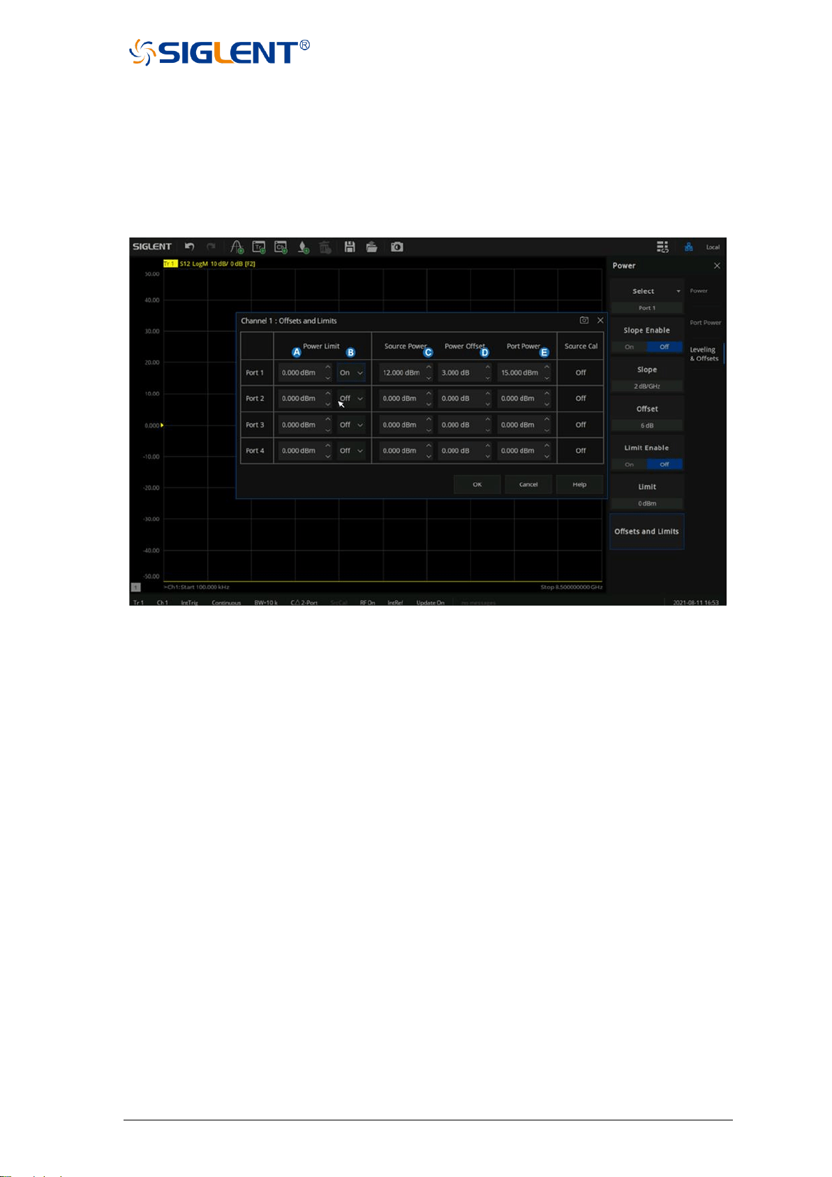
SNA5000A Vector Network Analyzer User Manual 30
1. On the UI interface, click the cell twice in succession and then enter the value in the pop-
up virtual numeric keyboard.
2. Press the Tab key on the front panel to make the focus fall on the cell you want to change,
press the number key +Enter on the front panel to set the value, or turn the knob to
change the value.
A. Global Power Limit. This sets a maximum source power level for individual test ports. This
value limits port power for all channels and all applications. Power levels that attempt to
exceed the power limit are clipped at the limit.
B. Power Limit Enable. Selects On indicate that power is limited to the adjacent value at the
specified source port and selects Off indicate that power is not limited to this value, but
the maximum power of the source.
C. Set the Source Power value.
D. Set the Power Offset value.
E. Set the Port Power value. The formula among Source Power, Power Offset, and Port
Power is: Source Power + Power Offset = Port Power
2.4 Sweep
Sweeping refers to the measurement of a series of consecutive data points against a series
of specified excitation values.
2.4.1 Points
Data points are the number of data samples representing the measured values at a single
excitation value. You can specify the number of data points that the vector network analyzer
measures in a sweep. The sweeping time of the vector network analyzer varies proportionally
with the number of points.

31 SNA5000A Vector Network Analyzer User Manual
Operating steps:
Press Sweep, use the knob or arrow keys to focus on the Sweep→Number of Points
parameter item, Enter the number of points required, Press ENTER to exit editing mode.
The number of data points collected by the vector network analyzer during the
measurement sweep can be set to any number between 1 and 100001.
Note: Maximum point limits may differ for some measurement classes.
• For maximum trace resolution, use the maximum data points.
• For faster throughput, use a minimum number of data points to provide an acceptable
resolution.
• To get the best number of points, look for values that do not differ significantly in the
measurement as you add points.
• To ensure accurate measurement calibration, ensure that the user uses the same number
of points for calibration and measurement.
• Points are the number of data items collected in one sweep. This number can be set
separately for each channel.
• To obtain high trace resolution for excitation values, select a larger point value.
• For high throughput, keep the smaller point value within the allowable trace resolution
range.
• For high measurement accuracy after calibration, use the same number of points as the
actual measurement.
2.4.2 Sweep type
Key operation:
Press Sweep, use the knob or arrow keys to focus on the Sweep→Sweep Type parameter
item. Press ENTER or Knob to enter the editing state, then move the cursor to the specified
position by up and down direction keys or Knob, set the sweep type to the required
measurement type, press ENTER or Knob to select the current option.
Sweep type:
• Linear frequency sweeping
• Log frequency sweeping
• Power sweeping
• CW time sweep
• Segmented sweeping
Linear frequency sweep: Set the measured abscissa frequency scale as a linear scale, and
keep the full frequency scale at equal intervals.

SNA5000A Vector Network Analyzer User Manual 32
Log frequency sweep: Set the measured abscissa frequency scale to log scale, To observe
a wider frequency range, the calibration interval in the full frequency
band is not uniform and presents periodic changes.
Power Sweep: The power sweep will increase or decrease the power of the source according
to the walk length. Power sweeping is used to characterize power-sensitive
circuits through measurements such as gain compression. In the Scan Type
dialog box, you can specify "Start Power", "Stop Power", "CW Frequency",
"Points".
Section sweeping: "Segmentation Sweep" activates a sweep consisting of frequency sub
scans (called segmentation). For each segment, you can define a
separate power level, IF bandwidth, IF bandwidth for each port, sweep
time, delay, sweep mode. After the measurement calibration has been
performed on the entire scan or all segments, the measurement values
of one or more segments can be calibrated.
In the segmented scan type, the vector network analyzer performs the following operations.
• Sort all defined segments in order of increasing frequency.
• Measurements were made at each point.
• Display a trace containing all retrieved data.
Limitations on segmented sweeping:
• The frequency range of one segment may not overlap with the frequency range of any
other segment.
• The number of segments is limited only by the combined data points of all segments in
the sweep.
• The frequency range of one segment may not overlap with the frequency range of any
other segment.
• The number of segments is limited only by the combined data points of all segments in
the scan.
Operating steps:
Press Sweep, Use the knob or arrow keys to focus on the Sweep→Sweep Type
parameter item. Parameter change mode:
1. Press ENTER or Knob to enter the state of parameter editing, then move the cursor to
the specified position by up and down arrow keys or Knob, set the scan type as Segment
Sweep, and press ENTER or Knob to select the current option.
33 SNA5000A Vector Network Analyzer User Manual
2. Press Sweep, use the knob or arrow keys to focus on the Segment Table parameter item.
Move the cursor to the specified position by up and down arrow keys or knobs, set Add
Segment, Insert Segment, Delete Segment and Delete All Segments to perform segment
operation. Select the segment scan table for segment setting and tick the corresponding
menu to display the corresponding contents in the following segment.
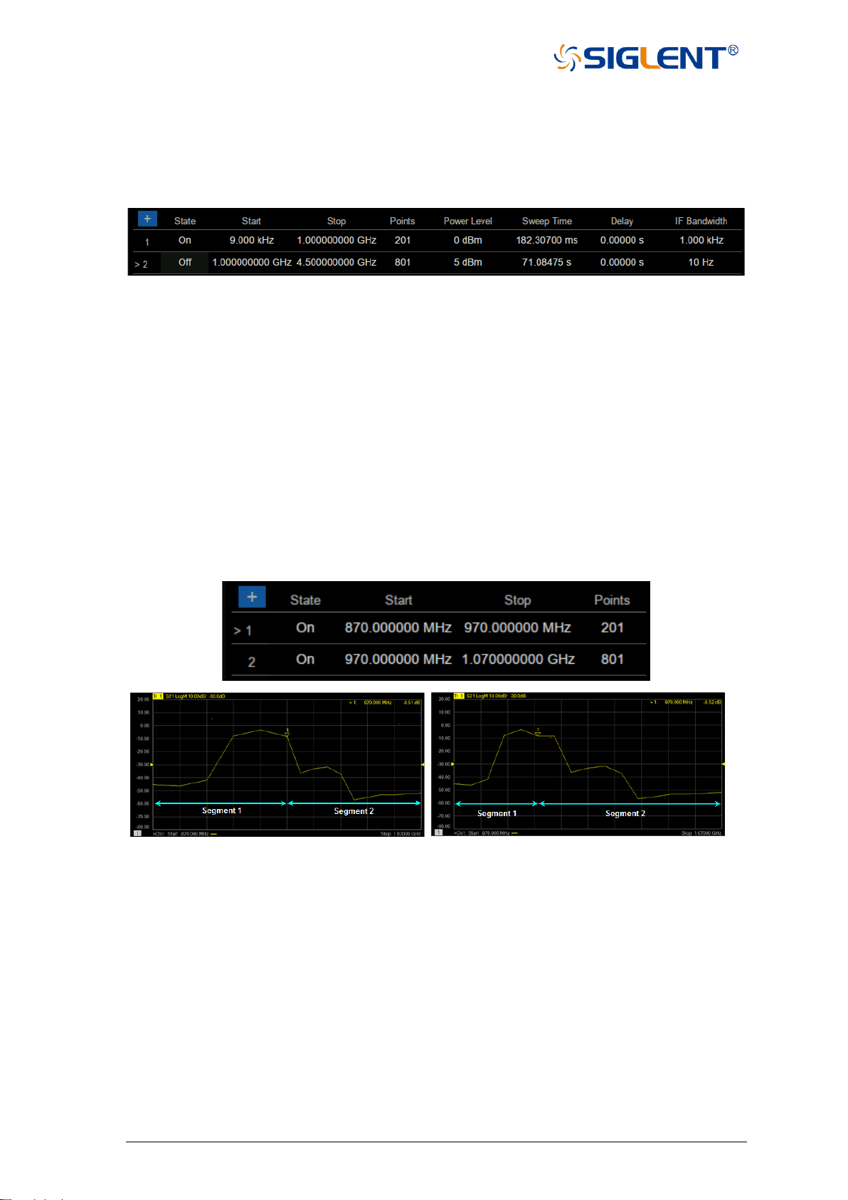
Figure 2-1 Sectional scan diagram
The X-axis spacing: In segment sweep mode, this feature will affect how the segment trace is
drawn on the screen. This function is in the sub-sweep table menu.
• When X-axis point spacing is not used, multi-segment sweeping traces may sometimes
result in many measurement points being squeezed into a narrower portion of the X-axis
• When X-axis point spacing is used, the X-axis position of each point needs to be selected
so that all measurement points are evenly distributed along the X-axis.
For example, suppose you have the following two sections:
X-point spacing is not used Use X-axis point spacing
Figure 2-2 Example of axis point spacing
2.5 Trigger
The trigger is the signal that causes the vector network analyzer to carry out the
measurement sweep. The vector network analyzer is flexible in the configuration of the trigger
function.
2.5.1 Trigger Settings
Operating steps:

SNA5000A Vector Network Analyzer User Manual 34
Press Trigger, use the knob or arrow keys to focus on the Trigger parameter item.
2.5.2 Trigger source
Operating steps:
Press Trigger, Use the knob or arrow keys to focus on the Trigger Source
parameter item. Press ENTER or the Knob to enter the parameter editing
state, then move the cursor to the specified position by the up and down arrow
keys or the knob, and press ENTER or the knob to select the current option.
Trigger source: These Settings determine the source of the trigger signal for all existing
channels. A valid trigger is generated only if the vector network analyzer is not
sweeping.
• Internal triggers: After the previous measurement is completed, the vector network
analyzer will immediately send a continuous trigger signal.
• Bus trigger: The vector network analyzer waits for the SCPI trigger instructions issued by
an external controller (PC).
• External trigger: Trigger signals generated by external devices received through the BNC
connector on the rear panel.
• Manual trigger: Manually send a trigger signal to the vector network analyzer. Available
only when you select “Manual” to trigger.
2.5.3 Trigger Range
Operating steps:
Press Trigger, Use the knob or arrow keys to focus on the Trigger Scope
parameter item. Press ENTER or the Knob to enter the parameter editing
state, then move the cursor to the specified position by the up and down arrow
keys or the knob, and press ENTER or the knob to select the current option.
• All channels: Triggers are sent to all triggerable channels. A trigger will sweep all channels
that can be triggered. (Default setting)
• Current channel: Triggers are sent to the current channel but after the current channel
completes, the channel increments to the next triggerable channel.
2.5.4 Channel Settings
Operating steps:
Press Trigger, use the knob or arrow keys to focus on the Trigger parameter
item. Press ENTER or the Knob to enter the parameter editing state, then
move the cursor to the specified position by the up and down arrow keys or
the knob, and press ENTER or the knob to select the current option.

35 SNA5000A Vector Network Analyzer User Manual
These settings determine the number of trigger signals that the channel will receive.
• Hold trigger: The channel does not accept any trigger signals.
• Single trigger: The channel receives a trigger signal and then enters the "hold" state.
Another way to trigger a single measurement: Set the trigger source to
"manual" and send a manual trigger. At this point, however, all channels
are set to single trigger.
• Continuous trigger: Channels accept an unlimited number of trigger signals.
• Hold all channels: All channels enter the hold state and do not accept any trigger signals.
• Restart: (Accessible only from the Trigger menu.) Channels that are in the Hold state are
set to be triggered once (The channel accepts a single trigger signal). All other
Settings are unaffected.
• A single trigger: The channel receives a trigger signal and then enters the "hold" state.
Another way to trigger a single measurement is to set the trigger source
to "manual" and send a manual trigger. At this point, however, all channels
are single.
• Restart: (Accessible only from the Trigger menu.) Channels that are in the “Hold“ state are
set to be a single trigger (This channel receives a single trigger signal). All other
settings are unaffected.
2.5.5 Trigger mode
Operating steps:
Press Trigger, use the knob or arrow keys to focus on the Trigger→Trigger Setup
parameter item. Press ENTER or the Knob to enter the parameter editing state. Then move
the cursor to the specified position by the up and down arrow keys or the knob, and press
ENTER or the knob to select the current option.
These settings determine the number of trigger signals that the channel will receive.
• Sweep trigger: Each "manual" or "external" trigger causes all traces of the shared source
port to be swept in the order specified below. In the case of a "single"
trigger, the count decrements by 1 after sweeping all traces in all
directions.
• Point trigger: Each "manual" or "external" trigger results in a measurement of a data point.
Subsequent triggers go to the same trace until it completes, The other traces
in the same channel are then swept in the order specified below. If it is a
"single" trigger, the count decreases by 1 after measuring all data points on
all trace lines in the channel.

SNA5000A Vector Network Analyzer User Manual 36
When multi-port calibration is on (requires multi-direction sweeping), the trace on the
screen will not be updated until all relevant directions have been swept. For example, when all
four 2-port S parameters are displayed:
a) If full 2-port calibration is on, triggering 1 will cause no trace to be updated.
b) When the calibration is off, triggering 1 will cause S11 and S21 updates. Trigger
2 will cause updates to S22 and S12.
Track scan sequence:
For all trigger modes, the trigger signal remains in the same channel until all traces in this
channel have been scanned, and then continue to trigger the next channel that is not in the
"hold" state.
The traces within each channel are always scanned in the following order:
The trace on the screen will not be updated when the multi-port calibration is turned on
(requiring multi-direction sweeping) until all relevant directions have been swept.
For example, when all four 2-port S parameters are displayed:
a) If full 2-port calibration is on, triggering 1 will cause no trace to be updated; Triggering
2 causes all S parameters to be updated.
b) When the calibration is off, triggering 1 will cause S11 and S21 to be updated;
Triggering 2 will cause S22 and S12 to be updated.
Track sweep sequence:
The trigger signal continues to be in the same channel for all trigger modes until all traces
in this channel have been swept. Then, it continues to trigger the next channel that is not in the
“Hold“ state.
The traces within each channel are always swept in the following order:
• Sweep traces in order of source ports. For example, in a channel with all four 2-port S
parameters, the source port 1 trace (S11 and S21) is swept simultaneously first. Then,
source port 2 traces (S22 and S12) are swept simultaneously.
2.5.6 External and auxiliary triggers
Both external and auxiliary triggers are used to synchronize the triggers of the vector
network analyzer with those of other devices.
Overview
Ready signal and trigger signal:
Ready signals are different from trigger signals. The ready signal is used to indicate that
the transmitting instrument is ready for measurement. The instrument receiving the ready
signal then sends a trigger signal indicating that the measurement will be made or that the
measurement has been completed. Usually, the slower instrument sends the trigger signal.

37 SNA5000A Vector Network Analyzer User Manual
• Measurement trigger input: This signal is easy to use, but has limited configuration
capabilities.
• Auxiliary trigger outputs: Connectors and signals are highly configurable and can be used
to synchronize with any number of devices.
Measurement trigger input
The trigger input connector is located on the back panel of the vector network analyzer.
These signals can be used when the vector network analyzer communicates with slower
instruments.
Operating Steps:
• The vector network analyzer sends a "ready" signal when it is ready for measurement
• The external device sends a trigger signal to the vector network analyzer when it is ready
for measurement
• Additional signals are provided on the vector network analyzer processor I/O to indicate
that the vector network analyzer sweep has been completed and the processor can be set
for the next measurement.
To make the vector network analyzer respond to measured trigger inputs or processor I/O
signals, select External on the “Trigger Settings“ tab on the “Source“ Settings. Also, on the
Trigger Settings tab, on the Range Settings, select whether an external trigger applies to all
channels (global) or one channel (local). The appropriate settings to apply are as follows:
Main trigger input:
Global/channel trigger delay - after receiving an external trigger, the start time of the sweep
will be delayed by the specified amount of time plus any inherent delay.
• When the trigger scope is "channel", the delay value is applied to the specified channel.
• When the Trigger Range is Global, the same delay value is applied to all channels.
The vector network analyzer receives the trigger input signal through the following connectors:
• Measure trigger input BNC connector: Trigger input on the rear panel.
• Processor I/O Pin 18 (needs to be changed).
Polarity:
High level: When the vector network analyzer is ready (trigger ready) and the TTL signal on
the selected input is "high", It triggers the vector network analyzer.
Low level: When the vector network analyzer is ready (trigger ready) and the TTL signal on the
selected input is "low", it triggers the vector network analyzer.

SNA5000A Vector Network Analyzer User Manual 38
Positive edge: When the vector network analyzer is ready, it will trigger on the next positive
edge. When set to accept a trigger before ready, if a positive edge has been
received since the last data acquisition, the vector network analyzer will trigger
immediately after ready
Negative edge: When the vector network analyzer is ready, it will trigger on the next negative
edge. When set to accept the trigger before ready, if a negative edge has
been received since the last data acquisition, the vector network analyzer will
trigger immediately after ready.
After receiving the trigger selection before being ready, the vector network analyzer will
move to the ready state (trigger ready), if any triggers have been received since the last data
fetch, the vector network analyzer will trigger immediately and the vector network analyzer will
remember only one trigger signal. All other signals will be ignored.
• If this check box is cleared, any trigger signals received by the vector network analyzer
before it is ready will be ignored.
• This feature is only available when a positive or negative edge trigger is selected.

39 SNA5000A Vector Network Analyzer User Manual
Auxiliary trigger
The auxiliary trigger connector is located on the back panel of the vector network analyzer.
When the external source is configured as an external device, the vector network analyzer will
automatically control all trigger settings. Do not set other trigger settings. The vector network
analyzer will start measuring when it receives a valid trigger signal from the specified trigger
source:
• Inside: Measurements begin immediately.
• Manual: Press the vector network analyzer "Trigger" button to start the measurement.
• External: The measurement starts when the measurement trigger input signal is received
from the external device. This must be configured separately.
The "Auxiliary Trigger Output" signal can be configured to be sent just before the
measurement is performed or just after the measurement is completed. When
communicating with an external source, the "Auxiliary Trigger Output" signal should be sent
after the measurement is completed to indicate that the external source can be set for the
next measurement.
Enable: When checked, the signal can be output to external devices using auxiliary connectors.
• Channel: This setting is controlled by the vector network analyzer “Preferences“ setting.
• Global: All secondary trigger settings apply to all channels. On the Trigger Settings tab,
set the "Each Point" setting, which also applies to all channels.
Channels: All secondary trigger settings will be applied to the specified channel and each
channel can be configured individually.
Auxiliary channel output (to device):
The following settings control the properties of the signal emitted from the “Auxiliary Trigger
Output“ connector on the back panel:
Polarity:
Positive pulse: the output pulse is positive.
Negative pulse: The output pulse is negative.
Location:
Before acquisition: Send pulses just before data collection begins.
After the acquisition: Pulses are sent immediately after data collection is completed.
Each point: When checked, trigger output can be sent for each data point, and when cleared,
trigger output can be sent for each sweep.

SNA5000A Vector Network Analyzer User Manual 40
Select "Auxiliary Trigger" - "Global" vector network analyzer preferences, On the "Trigger
Settings " tab, the "Dot " Settings are set. After that, this setting applies to all channels. When
multiple channels exist, the channel settings set last are used.
Pulse Duration: Specify the duration of a positive or negative output trigger pulse.
2.6 Data format
The data format is the method by which the vector network analyzer displays the
measured data graphically. Select the data format that corresponds to the information you want
to know about the test device.
2.6.1 Display format
Operating steps:
Press Format, Use the knob or arrow keys to focus on the Format parameter item. Press
ENTER or the Knob to enter the parameter editing state, then move the cursor to the specified
position by the up and down arrow keys or the knob, and press ENTER or the knob to select
the current option.
2.6.2 LF Cartesian coordinates display format
Nine of the twelve available data formats use rectangular displays to present
measurement data. This display is also known as Cartesian, XY, or linear coordinates. The
Cartesian coordinate display is especially suitable for clearly displaying the frequency
response information of the device-under-test (DUT).
• The excitation data (frequency, power, or time) is linearly scaled and displayed on the X-
axis
• The measured response data is displayed on the Y-axis
Log amplitude scheme:
• Display amplitude (no phase)
• Y: dB
• Typical measurements: Return loss, insertion loss, or gain
• Display phase (no amplitude)
Phase format:
The phase of the signal is measured relative to the calibration reference plane, within
a range of ±180 degrees.
• Y: Phase (degrees)
• Each 180-degree trace is "wrapped" for easy scaling
• Typical measurement: Linear phase shift.

41 SNA5000A Vector Network Analyzer User Manual
A phase:
• Same phase, but no 180-degree entanglement.
Note: Phase unwrapping is accomplished by comparing the phases of two adjacent data
points. If the phase difference between the two points is greater than 180 degrees, or
the DC offset phase of the first data point is greater than 180 degrees, then the phase
measurement may not be accurate.
Group delay format:
• Displays the transmission (propagation) time of signal in the device
• Y: Time (s)
• Typical measurement: Group delay
Linear amplitude scheme:
• Only positive values are displayed
• Y: No Unit (U, suitable for proportional measurements)
Watts (W, suitable for disproportionate measurements)
• Typical measurements: Reflection and transmission coefficients (amplitude), time domain
transformation
SWR format:
• Displays the reflection measurements calculated from the formula (1+ R)/(1-R), where R
is the reflection coefficient
• Valid for reflection measurements only
• Y: No units
• Typical measurements: SWR
Real number format:
• Show only the real part of the measured complex data
• Can display both positive and negative values
• Y: No units
• Typical measurements: Time domain, auxiliary input voltage signals for maintenance
purposes
Imaginary number format:
• Only imaginary parts of the measured data are displayed
• Y: No units
• Typical measurement: Network impedance matching
2.6.3 Polar coordinates
The polar coordinate format is used to view the amplitude and phase of the reflection
coefficients in S11 or S22 measurements.
You can use a cursor to display the following items:
• Linear or log amplitude (in dB)
• Phase (in degrees)
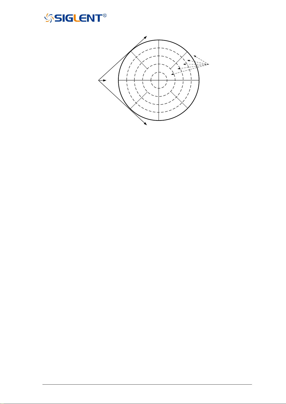
SNA5000A Vector Network Analyzer User Manual 42
Figure 2-5 Polar diagram
• The dotted circle indicates the reflection coefficient. The outermost circle represents the
reflection coefficient with a value of 1. The center of the circle represents the reflection
coefficient with a value of 0.
• The radial line shows the phase angle of the reflected signal. The right-most position
corresponds to the zero-phase angle (that is, the reflected signal has the same phase as
the incident signal). The phase differences of 90°, ±180°, and -90° correspond to the top,
leftmost, and bottom of the polar display, respectively.
2.6.4 Smith circle diagram
Smith diagrams are a tool for mapping complex reflectance coefficients to test the
impedance of equipment. In the Smith chart, the linear impedance plane is reshaped to form
a cyclic grid from which the resistance and reactance (R+ Jx) can be read.
You can use a cursor to display the following items:
• Resistance (in Ohms)
• Reactance as equivalent capacitance (in Ephraeras) or inductance (in Henrys)
0Ω
±180°
∞Ω
0°
90°
-90°
0.2
0.4
0.6
0.8
1.0
The magnitude of Γ
(reflection coefficient)
The phase Angle of the
reflected signal
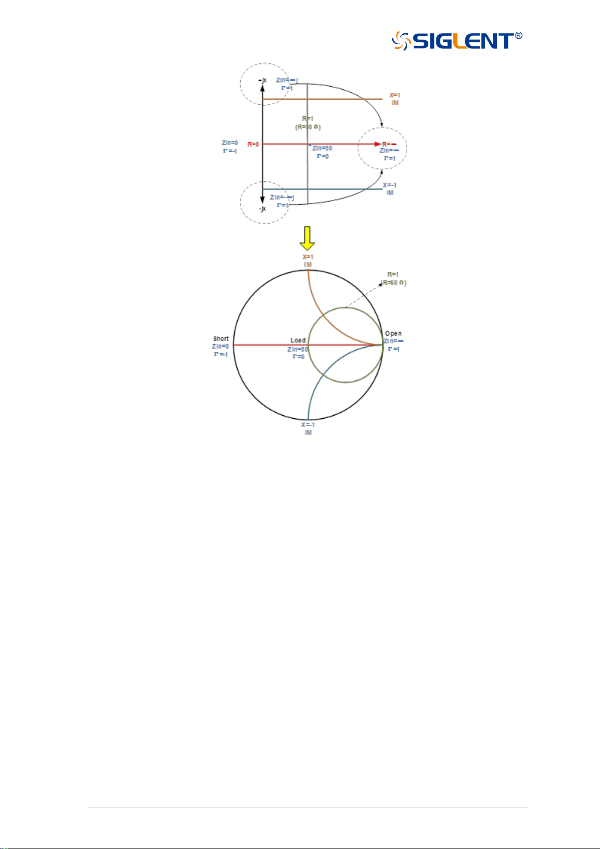
43 SNA5000A Vector Network Analyzer User Manual
Figure 2-6 Schematic diagram of Smith circle
There is also a Reverse Smith circle diagram (also called an Admittance Smith Chart):
Same as the standard Smith circle, with the following exceptions:
• The polar grid is reversed from right to left.
• Admittance (in Siemens) instead of resistance.
Smith diagram interpretation:
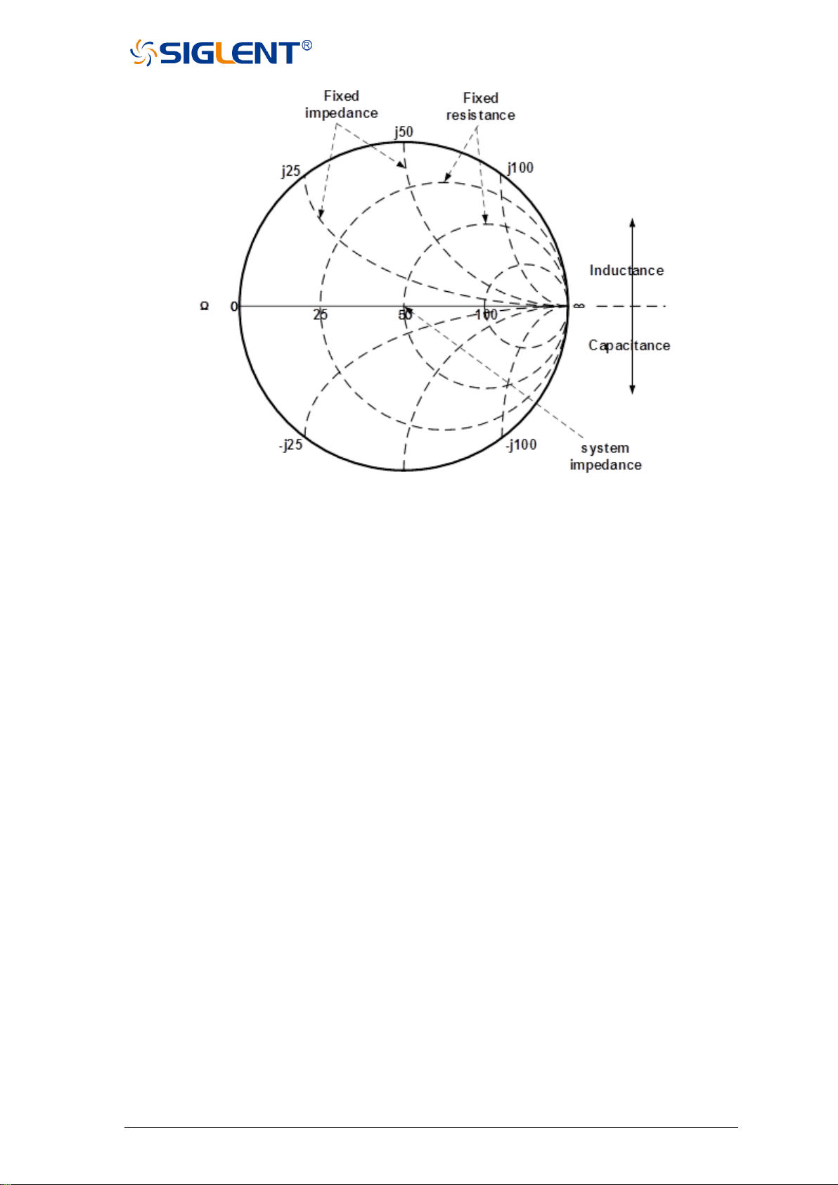
SNA5000A Vector Network Analyzer User Manual 44
Figure 2-7 Schematic diagram of the Admittance Smith chart
• Each point on the Smith chart represents a complex impedance (r±jx) consisting of a real
resistance (r) and an imaginary reactance (x).
• The horizontal axis (solid line) shows the real part of the difference between impedance
and resistance. The horizontal axis always represents the system impedance. The
rightmost value is infinite ohms (open path). The leftmost value is zero ohms (short circuit).
• The dotted circle intersecting the horizontal axis represents a constant reactance.
• A dashed arc tangent to the horizontal axis represents a constant impedance.
• The top half of Smith's circle is the region where the reactance component is positive and
hence inductance is generated.
• The lower half is the region where the reactance component is negative and therefore
generates capacitance.
2.7 Scale
2.7.1 Scale/reference level and position
The "Scale", "Reference Level", and "Reference Position" Settings (as well as the format)
determine how the data trace will appear on the vector network analyzer screen.
Operating steps:

45 SNA5000A Vector Network Analyzer User Manual
Press Scale, Use the knob or arrow keys to focus on the reference level and reference
position parameter items under the Scale menu bar. Press ENTER or the knob to enter the
parameter editing state, then move the cursor to the specified position by the up and down
arrow keys or the knob, and press ENTER or the knob to select the current option.
Scale: Sets the vertical indexing value of the rectangular coordinate display format. In polar
coordinates and Smith chart formats, the scale sets the value of the outer perimeter.
Range: 0.001 dB/div to 1000 dB/div.
Automatic scaling: Automatically sets the vertical indexing value and reference value to fit
the working data trace in the screen grid area. The excitation value and
reference position are not affected. The vector network analyzer
determines the minimum possible scaling factor that will allow all display
data to appear on the 80% vertical grid. The selected reference values
center the trace on the screen.
All autoscaling: Automatically scales all data traces in the working window to fit vertically into
the grid area of the screen.
Reference level: Sets the value of the guide in rectangular format. Range: -1000 dB to 1000
dB. In polar coordinates and Smith's circle chart formats, the reference level
does not apply.
Reference position: Sets the position of the guide in Rectangular coordinate format. Zero is
the bottom line and 10 is the top line. The default position is 5 (middle of
the screen). Reference positions do not apply in polar coordinates and
Smith chart formats.
2.7.2 Scaling coupling
When “Scale Coupling“ is enabled, tracks of the same format will have the same “Scale“,
“Reference Level“, and “Reference Position“. You can choose to couple the scales for traces
in the same window, for all traces in all Windows, or uncouple them.
Operating steps:
Press Scale, use the knob or arrow keys to focus on the Scale→Scale Coupling
parameter item. Press ENTER or Knob to enter the editing state, select Off/Window/All, then
move the cursor to the specified position by up and down arrow keys or Knob, press ENTER
or Knob to select the current option
Note: Traces of the same format have the same scale, reference level, and reference position.
Coupling Method:
Close: No coupling. Each trace is scaled individually. This is the default setting.
Window: All traces of the same format in each selected window share the same scale settings
All: Coupled between all selected windows, all traces of the same format in all selected

SNA5000A Vector Network Analyzer User Manual 46
windows share the same scale settings.
• When window or full coupling is enabled, the scale settings for the working trace will be
adopted by other coupling traces of the same format
• If traces of a different format exist, all traces of that format will be set as the least numbered
trace in that format
• Once enabled, the scale settings for all coupling traces of the same format can be changed
with any coupling trace in the working state
Selected Windows:
Available when selecting a window or all methods. The selected window participates in
scaling coupling. By default, all windows are selected. Cancel the check box to disable zoom
coupling for this window.
About "Auto Scaling" and "Scaling Coupling":
Automatic scaling using the coupling method affects the work trace in the work window.
All traces coupled to this trace will be set with the new scale of the working trace. This will
cause some traces to not appear on the screen.
Full automatic scaling using the coupled method
• Close: All traces in the working window are automatically scaled separately.
• Window: All traces in each selected window are automatically scaled to conform to a
common set of scaling factors.
• All: All traces in all selected Windows are automatically scaled to conform to a common
set of scaling factors.
2.7.3 Electrical delay
Electrical delay is a mathematical function that simulates the variable length of a lossless
transmission line. Linear phase shifts through the device can be compensated using the
electrical delay function. Use this feature to determine only the linear phase deviation of the
device. Electrical delay can be set separately for each measuring trace.
Operating steps:
Press Scale, use the knob or arrow key to bring focus to the Electrical Delay parameter
item. Press ENTER or Knob to enter the editing state. After the editing is completed, move the
cursor to the specified position by up and down direction keys or Knob. Press ENTER or Knob
to select the current option.
Delay time: Specifies the value of the delay added or removed, expressed in time or distance.
This compensates for the linear phase shift through the device. Electrical delay
can be set separately for each measuring trace.

47 SNA5000A Vector Network Analyzer User Manual
Speed coefficient: Specify the velocity factor applied to the device media inserted after
measurement calibration. The value is 0.66 for polyethylene insulated
cables and 0.7 for PTFE insulators.1 corresponds to the speed of light in
a vacuum.
Distance unit: Select meters, inches, or feet. When you change this value, the step size does
not change automatically.
2.7.4 Amplitude offset and amplitude slope
The "amplitude offset" allows the amplitude (rather than phase) data to be offset by a fixed
or slope value in Db. The amplitude offset setting affects only the work trace. If the display
format is "Linear Amplitude" or "Real Number" (unitless), the dB is converted and the correct
offset is implemented.
Operating steps:
Press Scale, use the knob or arrow keys to bring focus to the Constants→Mag Offset/
Mag Slope parameter item.
Press ENTER or Knob to enter the editing state. After the editing is completed, move the
cursor to the specified position by up and down direction keys or Knob. Press ENTER or Knob
to select the current option.
Amplitude deviation: Offset the entire data trace at the specified value.
Margin slope: Offset the data trace by some value that changes with frequency. The offset
slope starts at 0 Hz.
2.7.5 Phase deviation
Phase offset mathematically adjusts the phase measurement to a specified degree (up to
360°). This feature can be used in the following ways:
• Improved display of phase measurements. This is the same way as changing the
reference level in the amplitude measurement. Change the phase response to the center
or align the response on the screen.
• Simulate Projection phase shift in measurements. For example, if you know that you need
to add a cable and that the length of the cable will add a certain phase shift to the
measurement, you can use a phase shift to increase the length and simulate the entire
device measurement.
Key operation:
Press Scale, use the knob or arrow keys to bring focus to the Constants→Phase Offset
parameter item. Press ENTER or Knob to enter the editing state. After the editing is completed,
move the cursor to the specified position by up and down direction keys or Knob. Press ENTER
or Knob to select the current option.
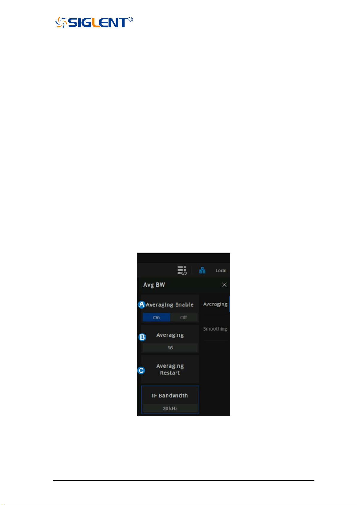
SNA5000A Vector Network Analyzer User Manual 48
2.8 Avg BW
2.8.1 Overview
The dynamic range is the finite difference between the maximum input power level and
the minimum measurement power level (noise floor) of the analyzer. In evaluating a
characteristic accompanied by a large change in the amplitude (the start and stop band of a
filter for example), it is important to increase the dynamic range. The noise floor can be reduced
by narrowing the IF bandwidth or turning on Sweep Averaging.
For minimizing very low noise, Averaging is more effective than reducing IF bandwidth.
Generally, Averaging takes slightly longer than IF bandwidth reduction to lower noise,
especially if many averages are required. Also, changing the IF bandwidth after calibration
results in uncertain accuracy.
2.8.2 Averaging
Averaging is a feature that the VNA averaging on each data point before stepping to the
next data point. You determine the number of measurements by setting the averaging factor.
The higher the averaging factor, the greater the amount of noise reduction.
Averaging setting:
Press the ”Avg BW” key, then enter the Averaging and Bandwidth menu.
Figure 2-8 Avg BW menu
A. Averaging Enable.
B. Sweep Averaging factor. (an integer between 1 and 999)
C. Averaging Restart. Restart the Sweep Averaging from 1.
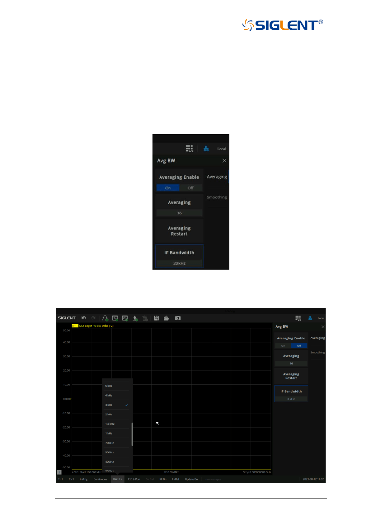
49 SNA5000A Vector Network Analyzer User Manual
2.8.3 IF Bandwidth
The received signal of VNA is converted from its source frequency to a lower intermediate
frequency (IF). Reducing the IF receiver bandwidth reduces the effect of random noise on a
measurement. Each tenfold reduction in IF bandwidth lowers the noise floor by 10 dB. However,
narrower IF bandwidths cause longer sweep times.
IF Bandwidth setting:
1. Using the Softkey for setting: Press the ”Avg BW” key, Press “Avg BW” > Averaging > IF
Bandwidth > Enter the IF Bandwidth value.
Figure 2-9 Set the IF from the menu bar
2. Using a mouse for setting: Click the "BW=xx" icon on the menu bar and select IF
Bandwidth.
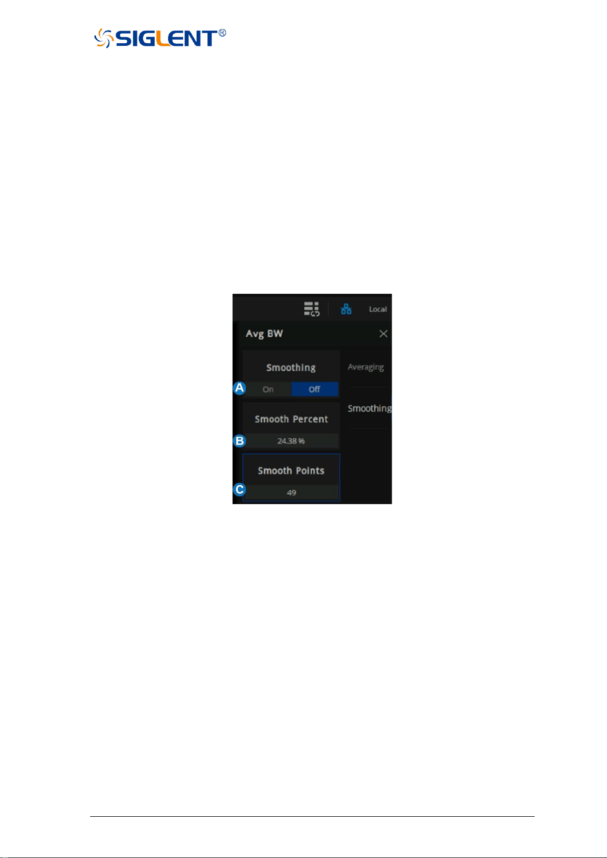
SNA5000A Vector Network Analyzer User Manual 50
Figure 2-10 Set the IF from the status bar
2.8.4 Smoothing
Trace smoothing averages several adjacent data points to smooth the displayed trace.
The number of adjacent data points that get averaged together is also known as the smoothing
aperture. You can specify the aperture as either the number of data points or the percentage
of the x-axis span.
Trace Smoothing reduces the peak-to-peak noise values on broadband measured data. It
smooths trace noise and does not increase measurement time significantly.
Smoothing setting:
Using the Softkey for setting: Press the ”Avg BW” key, “Avg BW” > Smoothing then enter
the Smoothing menu.
Figure 2-11 Smoothing menu
A. Smooth On|Off When is On, applies smoothing to the displayed trace.
B. Percent of Smooth: Specify the percent of the swept stimulus span to smooth. For
example, for a trace that contains 100 data points, and a smoothing percent of span =
11%, then the number of data points that are averaged is 11.
C. Smooth Points: Specify the number of adjacent data points to average.
Tips:
• Start with a high number of display points and reduce until you are confident that the trace
is not giving misleading results.
• Do not use smoothing for high-resonance devices, or devices with wide trace variations.
It may introduce misleading information.
• Smoothing is set independently for each trace.

51 SNA5000A Vector Network Analyzer User Manual
2.9 Preset instructions
Invokes preset Settings to restore system Settings to the specified just started state.
Operating instructions:
◆ Preset types are available through Preset→Preset Option, Select “Default”, “Last”, or
“User“.
◆ Press the Preset key, and the device invokes either default Settings or user Settings.
Table2-1 Some default setting values
Parameter name
Parameter value
RF Power
RF state
ON
RF level
0 dBm
Signal output port
Port 1
Port coupling
ON
Frequency
Frequency range
100 kHz-8.5 GHz
Frequency step size
42.4995 MHz
Frequency points
201
Sweeping
Sweeping points
201
Sweeping type
Linear frequency
Sweeping time delay
0 s
Sweeping mode
automatic
Trigger
Trigger mode
continuous
Trigger source
internal
Measurement
S parameter
S11
Display format
Data display format
Log Mag
Scale
Scale
10 dB
Reference level
0 dB
reference position
5
Scale coupling
OFF
Delay time
0 s
Delay distance
0 m
Distance unit
meter
Speed coefficient
1
System impedance
50 Ω
Phase deviation
0°
Amplitude deviation
0 dB
Average
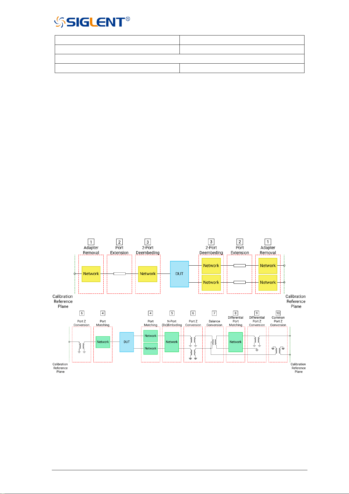
SNA5000A Vector Network Analyzer User Manual 52
Average state
OFF
Smooth state
OFF
Calibration
Calibration state
unloaded calibration data
3 Measurement calibration
3.1 Overview
Usually, DUTs can't be measured directly and accurately due to cabling, adapters,
probes, and more. Calibration, compensation, and fixture simulation are introduced to help
achieve higher accuracy. These functions meet different measurement requirements, but
they all can be expressed as a matrix multiplication of the scattering parameter matrix and a
specific compensation matrix. The order of the matrix multiplication has a large influence on
the result. So it's important to understand the order of applying these functions and to design
a suitable physical connection to the DUT and expected measurement network.
Internal source power calibration and receiver calibration are applied before the
scattering parameter calculation, and the S parameter calibration is applied to the calculation
results. This provides the highest measurement accuracy at the calibration reference plane.
From the reference plane, the order of applying functions is as follow:
Figure 3-1 The order of applying functions
At first, adapter removal/insertion, port extension, 2-port de-embedding are applied to
remove the needless networks in the physical connections of the DUT and move the
measurement plane to the DUT. Then, Port match, N-port embedding/de-embedding, port
impedance conversion are used to embed or de-embed expected virtual networks. If balance
scattering parameters are measured, balance conversion, differential port match, differential
port impedance conversion, common port impedance conversion can be helpful if needed.

53 SNA5000A Vector Network Analyzer User Manual
3.2 Calibration type
The following table is a comparison of some common S-parameter calibration types:
Table 3-1 S-parameter calibration types
Calibration type
precision
Allow pass-through methods
TRL
Very high
All, except the unknown direct
SOLT
high
All
Enhanced Response
high
Defined through or flush through (zero-
length through)
Port 1 (reflection)
high
Not Applicable
Open Circuit Response/
Short Circuit Response
low
Not Applicable
Direct Response
low
Known through or flush through (zero-
length through)
The following are the actual S-parameter calibration types used by this vector network analyzer.
Table 3-2 The vector network analyzer S parameter calibration types
Port number
Calibration type
Calibration item
Port 1
Response (Open)
Open, Load (optional)
Response (Short)
Short, Load (optional)
OSL
Open, Short, Load
Port 2
Response (Thru) 1→2
Thru, Isolation (optional)
Response (Thru) 2→1
Thru, Isolation (optional)
Enhanced Response (Thru) 1→2
Port1:Open, Short, Load
Thru, Isolation (optional)
Enhanced Response (Thru) 2→1
Port2:Open, Short, Load
Thru, Isolation (optional)
SOLT
Port1: Open, Short, Load
Port2: Open, Short, Load
Thru, Isolation (optional)
SOLR
Port1: Open, Short, Load
Port2: Open, Short, Load
Unknown Thru, Isolation (optional)
TRL
Port1: Reflect (Open or Short)
Port2: Reflect (Open or Short)
Thru, Line
TRL:

SNA5000A Vector Network Analyzer User Manual 54
Application: Used to precisely calibrate any pair of ports when no calibration kits are readily
Available.
Note: Difference matching calibration may be required (Delta Match Cal)
Overall accuracy: Very high
Calibration kits required: Straight, reflection, line, or similar combination
Corrected system error:
• Directivity
• Isolation
• Frequency response
transmission tracking
• Source match
• Load match
• Frequency response reflection
tracking
SOLT:
Application: Used to accurately calibrate any number of ports
Overall accuracy: High
Required calibration kits: short circuit, open circuit, load, through) or ECAL electronic
calibration parts module
• Directivity
• Isolation
• Frequency response
transmission tracking
• Source match
• Load match
• Frequency response reflection
tracking
Enhanced Response:
Application: Calibrate two ports when only one direction (forward or reverse) is needed for
measurement. Because no secondary scanning is required, the measurement is
faster.
• The reflection calibration element (open, short circuit, or load) is connected to
the source port to be calibrated.
• The defined through-through or flush through-through calibrator kits are
connected between port pairs.
• The mechanical calibration kit is much faster than the SOLT. You can also use
ECAL.
To select an enhanced response, do the following:
Keys operation:
Press Cal, using the knob or arrow keys, to focus on the Cal→Basic Cal parameter
item. Select port1 & port2 from the interface menu, Select Enhanced Response
1→2 or Enhanced Response 2→1 in the Cal Type, Press ENTER or the knob to
select the current option.
Overall accuracy: High

55 SNA5000A Vector Network Analyzer User Manual
Required calibration kits: Short circuit, open circuit, load, defined through or flush through
Corrected system error:
• Directivity (Source port)
• Isolation
• Frequency response
transmission tracking (receiver
port)
• Source match (source port)
• Load matching (receiver port) is
used only to generate
transmission trace items
• Frequency response reflection
tracking (source port)
One port (reflection):
Application: Used to accurately calibrate any test port suitable for reflection measurement only
Overall accuracy: High
Required calibration kits: Short circuit, open circuit, and load or ECAL module
Corrected system error:
• Directivity
• Frequency response reflection
tracking
• Source match
Open circuit response/short circuit response:
Application: Quick calibration of any test port suitable for reflection measurement only
Overall accuracy: Low
Calibration kits required: Open circuit or short circuit.
Corrected system error:
• Frequency response reflection tracking
Direct/Transport Tracking (isolation optional):
Application: Quick calibration of any pair of test ports suitable for transmission measurements
only. Isolation calibration is generally not recommended.
Overall accuracy: Low
Required calibration kit: Through
Isolation: Each load corresponds to a vector network analyzer test port.
Corrected system error:

SNA5000A Vector Network Analyzer User Manual 56
• Isolation
• Frequency response
transmission tracking
Power calibration types: Transmitter calibration (internal source power calibration) and
receiver calibration.
3.3 S parameter calibration
3.3.1 S parameter calibration Kit management
3.3.1.1 Overview
For most applications, the default calibration kit models provide sufficient accuracy for your
calibration. However, several situations may exist that would require you to create a custom
calibration kit:
• Using a connector interface different from those used in the predefined calibration kit
models.
• Using standards (or combinations of standards) that are different from the predefined
calibration kits. For example, using three offset SHORTs instead of an OPEN, SHORT,
and LOAD to perform a 1-port calibration.
• Improving the accuracy of the models for predefined kits. When the model describes the
actual performance of the standard, the calibration is more accurate. For example, A 7
mm LOAD is determined to be 50.4 Ω instead of 50.0 Ω.
• Modifying the THRU definition when performing a calibration for a non-insertable device.
• Performing a TRL calibration.
Operation instructions:
Press “Cal” on the front panel, Cal > Cal >Cal Kit to enter the Manage Cal Kits page. You can
edit, import, and create or delete calibration kits.
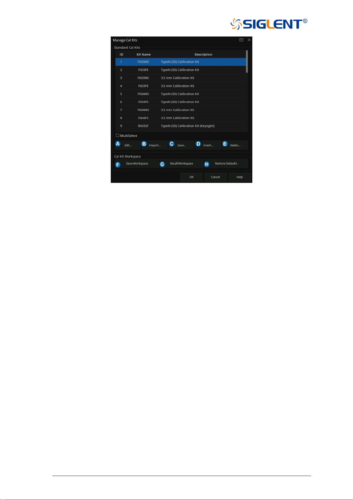
57 SNA5000A Vector Network Analyzer User Manual
Figure 3-2 Manage Cal Kits
A. Edit the Existing Cal Kit.
B. Import the customized Cal Kit.
C. Save the existing Cal kits and change the file name.
D. Create a new custom Cal Kit.
E. Select the Cal Kit.
F. Save the current Cal kits (both factory and custom).
G. Recall the Cal Kits.
H. Restore the default factory Cal Kits.
3.3.1.2 Connector Tab
At the bottom of each Tab, 'OK' is used to save the edited file, and 'Cancel' is used to close the
calibration suite edit session and the file will not be saved. “Help” is used to view the Help
documents.
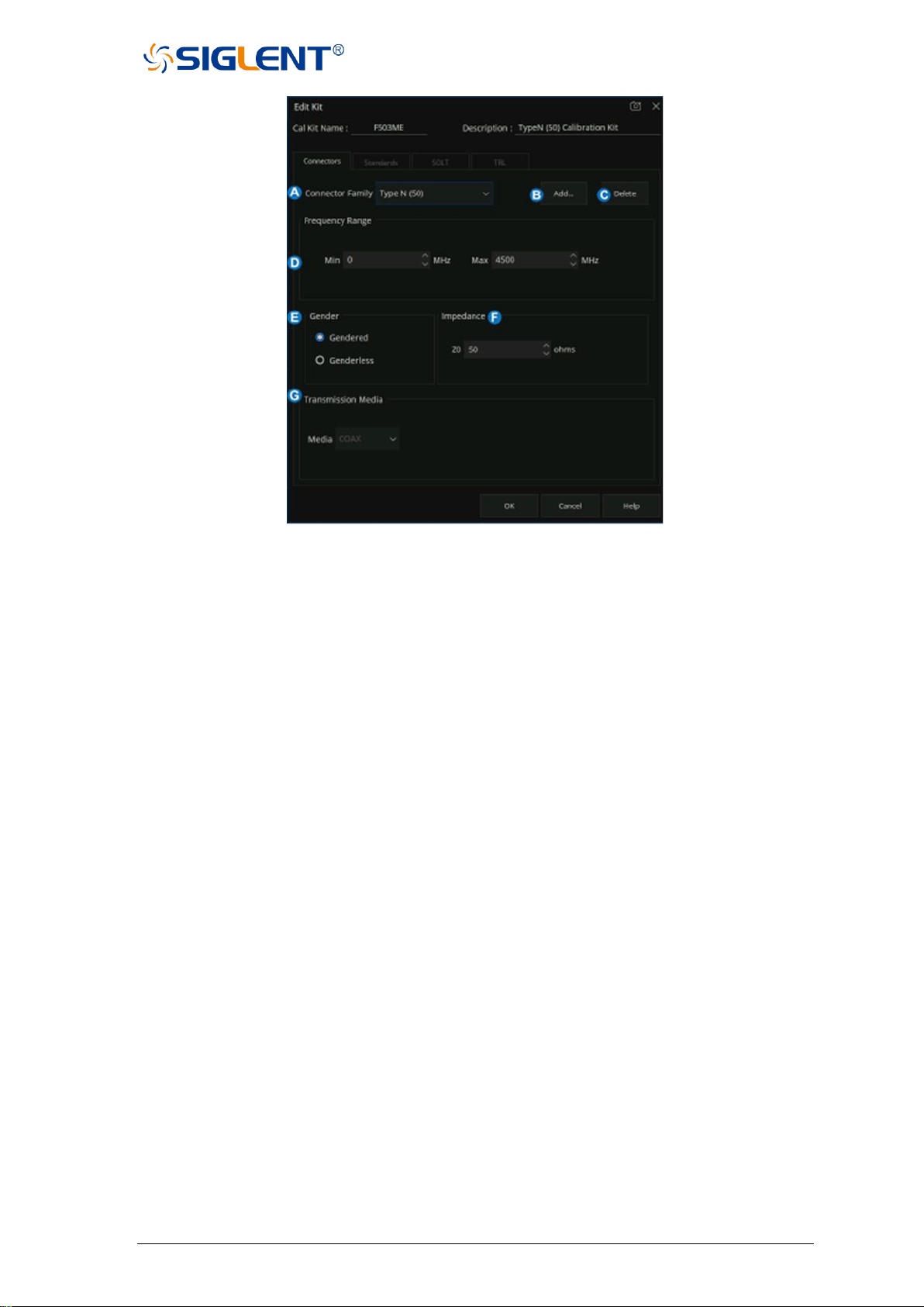
SNA5000A Vector Network Analyzer User Manual 58
Figure 3-3 The Connectors Tab interface
A. Connector Family: Click the down arrow to select the connector family associated with
the Cal Kit.
B. Add: Starts the Add Connector dialog box which allows you to add a new connector type
to the calibration kit.
C. Select: The selected connector family.
D. Frequency Range: Define the lowest and the highest frequency at which the standard is
used for calibration.
E. Gender: Gendered or Genderless.
F. Impedance: Specify the impedance of the standard.
G. Transmission Media: The medium of the connector, COAX or WAVEGUIDE
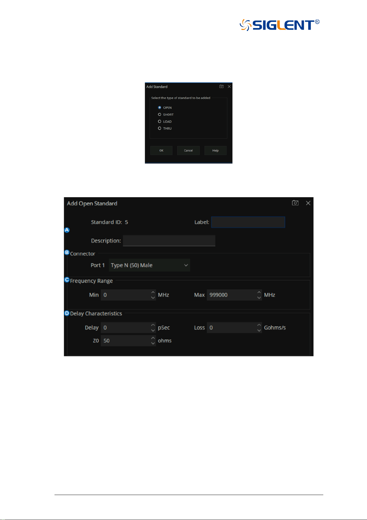
59 SNA5000A Vector Network Analyzer User Manual
3.3.1.3 Standards Tab
Allows you to Add, Edit, or Delete cal standards in a cal kit.
1) In the "Standard" tab, click "Add" to add the Standard sample.
Figure 3-4 add standard interface
2) Standards dialog box help, the following fields apply to ALL standard types.
Figure 3-5 The help dialog of the Standard
A. Identification
Standard ID: Number in list of standards
Label: Type of standard. This usually appears in prompts for standards.
Description: Description of standard.
B. Connector
Indicates the type and gender (Male, Female, None) of the standard.
Thru and Isolation standards have two connectors.
C.Frequency Range
Min: Defines the lowest frequency at which the standard is used for calibration.
Max: Defines the highest frequency at which the standard is used for calibration.
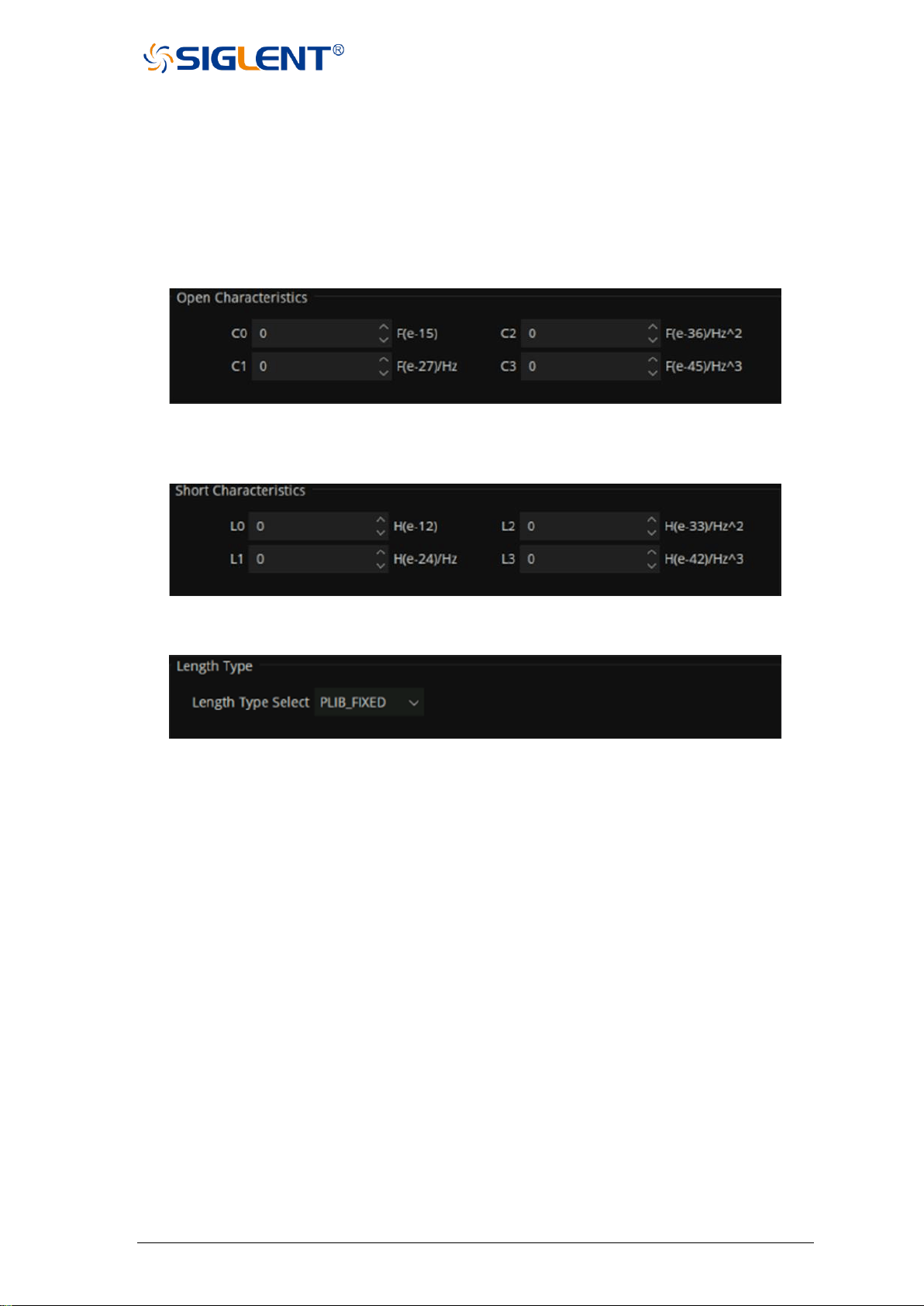
SNA5000A Vector Network Analyzer User Manual 60
D. Delay Characteristics
Delay: Defines the one-way travel time from the calibration plane to the standard in seconds.
Z0: Defines the impedance of the standard.
Loss: Defines energy loss in Gohms, due to skin effect, along a one-way length of coaxial cable.
Open Standard
C0, C1, C2, C3: Specify the fringing capacitance.
Figure 3-6 Open Characteristics
Short Standard
L0, L1, L2, L3: Specify the residual inductance.
Figure 3-7 Short Characteristics
Load Standard
Figure 3-8 load Characteristics
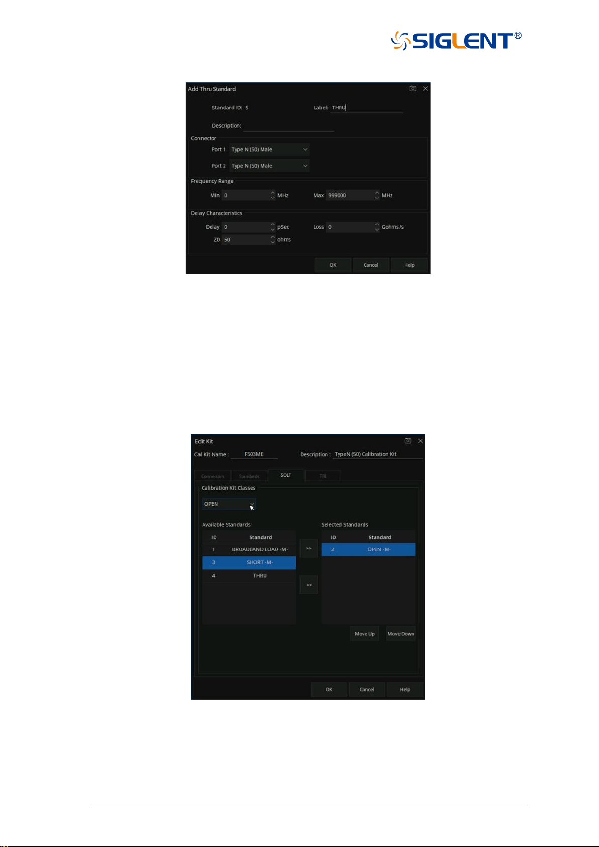
61 SNA5000A Vector Network Analyzer User Manual
THRU Standard
Figure 3-9 THRU Characteristics
3.3.1.4 SOLT Tab
Allows you to assign single or multiple standards to SOLT Calibration Classes.
1) For each Cal Kit Class, select Available Standards from the left list, then click >> to copy
the standard to the Cal Kit
2) Use Move Up and Move Down to change the ORDER of the standards.
Figure 3-10 SOLT Tab dialog box
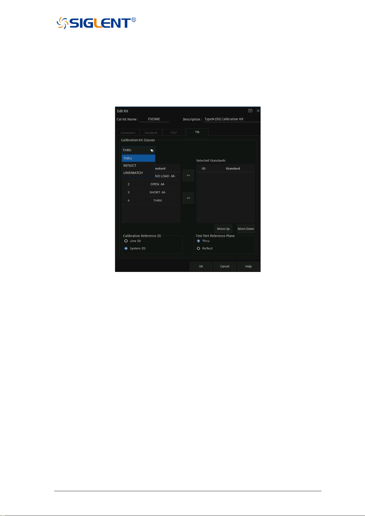
SNA5000A Vector Network Analyzer User Manual 62
TRL Tab
Allows you to assign single or multiple standards to Calibration Classes.
1) For each Cal Kit Class, select Available Standards from the left list, then click >> to copy
the standard to the Cal Kit.
2) Use Move Up and Move Down to change the ORDER of the standards.
Figure 3-11 TRL dialog box
A. TRL THRU
All THRU calibration methods are supported in a TRL Cal EXCEPT Unknown Thru.
• The THRU standard can be either a zero-length or non-zero length. However, a zero-
length THRU is more accurate because it has zero loss and no reflections, by definition.
• The THRU standard cannot be the same electrical length as the LINE standard.
• If the insertion phase and electrical length are well-defined, the THRU standard may be
used to set the reference plane.
• The THRU standard and LINE standard have the same characteristic impedance and are
perfectly matched. They define the reference impedance of the calibration.
• If a THRU standard with the correct connectors is NOT available, an adapter removal cal
can be performed.
B. TRL REFLECT
• The REFLECT standard can be anything with a high reflection, as long as it is the same
when connected to one or more VNA ports.
• The REFLECT standard on each port is identical.
• The actual magnitude of the reflection need not be known.
• The phase of the reflection standard must be known within 1/4 wavelength.
• If the magnitude and phase of the reflection standard are well-defined, the standard may
be used to set the reference plane

63 SNA5000A Vector Network Analyzer User Manual
C. TRL LINE
The LINE and THRU standards establish the reference impedance for the measurement after
the calibration is completed. TRL calibration is limited by the following restrictions of the LINE
standard
• Must be of the same impedance and propagation constant as the THRU standard.
• The electrical length need only be specified within 1/4 wavelength.
• Cannot be the same length as the THRU standard.
• A TRL cal with broad frequency coverage requires multiple LINE standards. For example,
a span from 2 GHz to 26 GHz requires two line standards.
• Must be an appropriate electrical length for the frequency range
D. TRL MATCH
If the LINE standard of appropriate length or loss cannot be fabricated, a MATCH standard
may be used instead of the LINE.
• The MATCH standard is a low-reflection termination connected to both Port 1 and Port 2.
• The MATCH standard may be defined as an infinite length transmission line OR as a 1-
port low reflect termination, such as a load.
• When defined as an infinite length transmission line, both test ports must be terminated
by a MATCH standard at the same time. When defined as a 1-port load standard, the
loads are measured separately. The loads are assumed to have the same characteristics.
• The impedance of the MATCH standard becomes the reference impedance for the
measurement. For best results, use the same load on both ports. The load may be defined
using the data-based definition, the arbitrary impedance definition, or the fixed load
definition.
E. Calibration Reference Z0
• System Z0: The system impedance is used as the reference impedance. Choose when
the desired test port impedance differs from the impedance of the LINE standard. Also,
choose when skin effect impedance correction is desired for coax lines.
• Line Z0: The impedance of the line standard is used as the reference impedance or center
of the Smith Chart. Any reflection from the line standard is assumed to be part of the
directivity error.
F. Test Port Reference Plane
• Thru Standard: The THRU standard definition is used to establish the measurement
reference plane. Select if the THRU standard is zero-length or very short.
• Reflect Standard: The REFLECT standard definition is used to establish the position of
the measurement reference plane. Select if the THRU standard is not appropriate AND
the delay of the REFLECT standard is well defined.
3.3.1.5 Greate a custom Cal Kit
There are two methods to create a custom Cal Kit:
Method 1:Create custom Cal Kit based on existing Cal kits
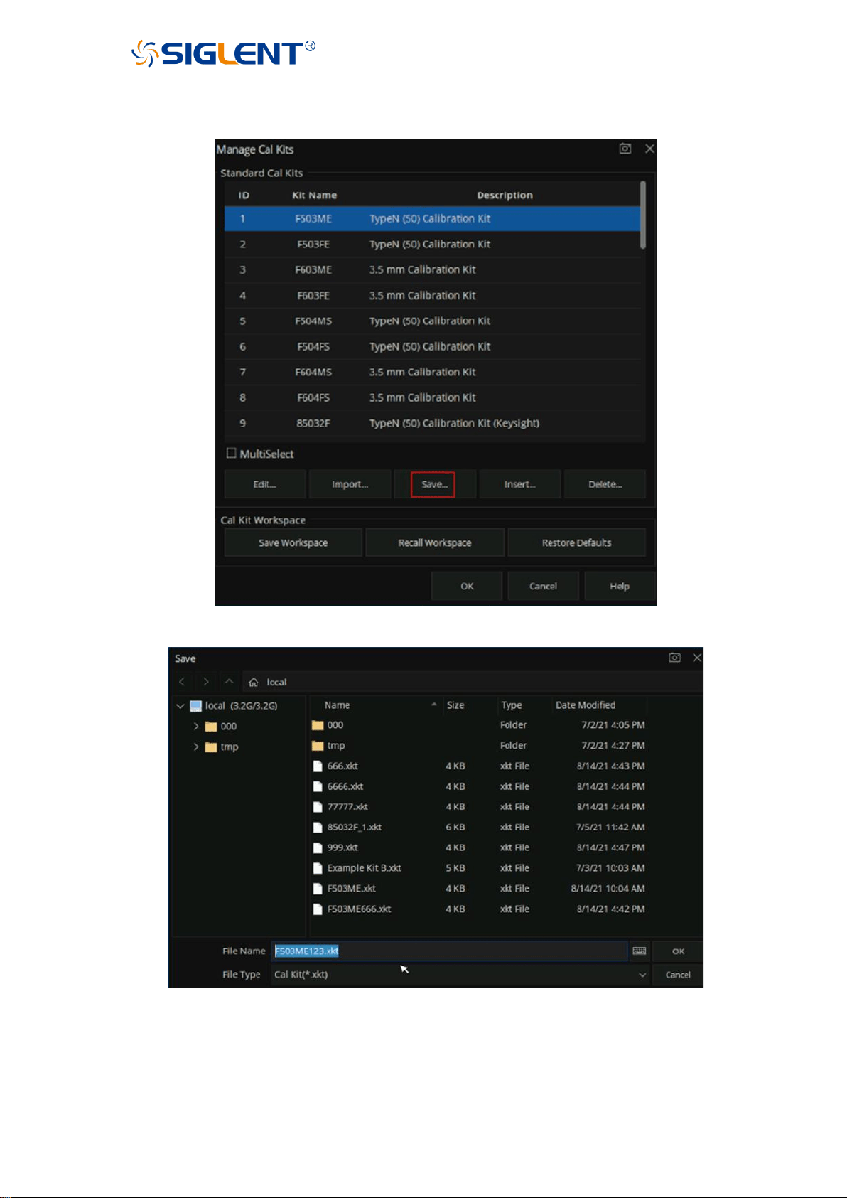
SNA5000A Vector Network Analyzer User Manual 64
1. Press “Cal” > Cal > Cal Kit > F503ME > Save . Select the existing F503ME Cal Kit then
save it to a local file named ”F503ME123.xkt”.
Figure 3-12 Creating a Custom Cal Kit dialog box
Figure 3-13 Save the ECal Kit
2. In the Manage Cal Kits dialog box, click "Import" to Import the new calibration
"F503ME123.xkt".
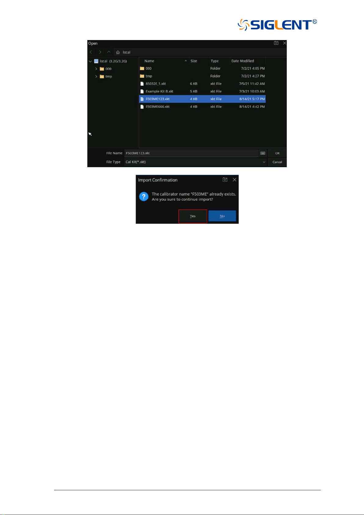
65 SNA5000A Vector Network Analyzer User Manual
Figure 3-14 Import the new ECal Kit
3. Select the newly imported calibration, click "Edit" to enter the calibration editing interface,
and modify the calibration name as "F530ME-ABC".
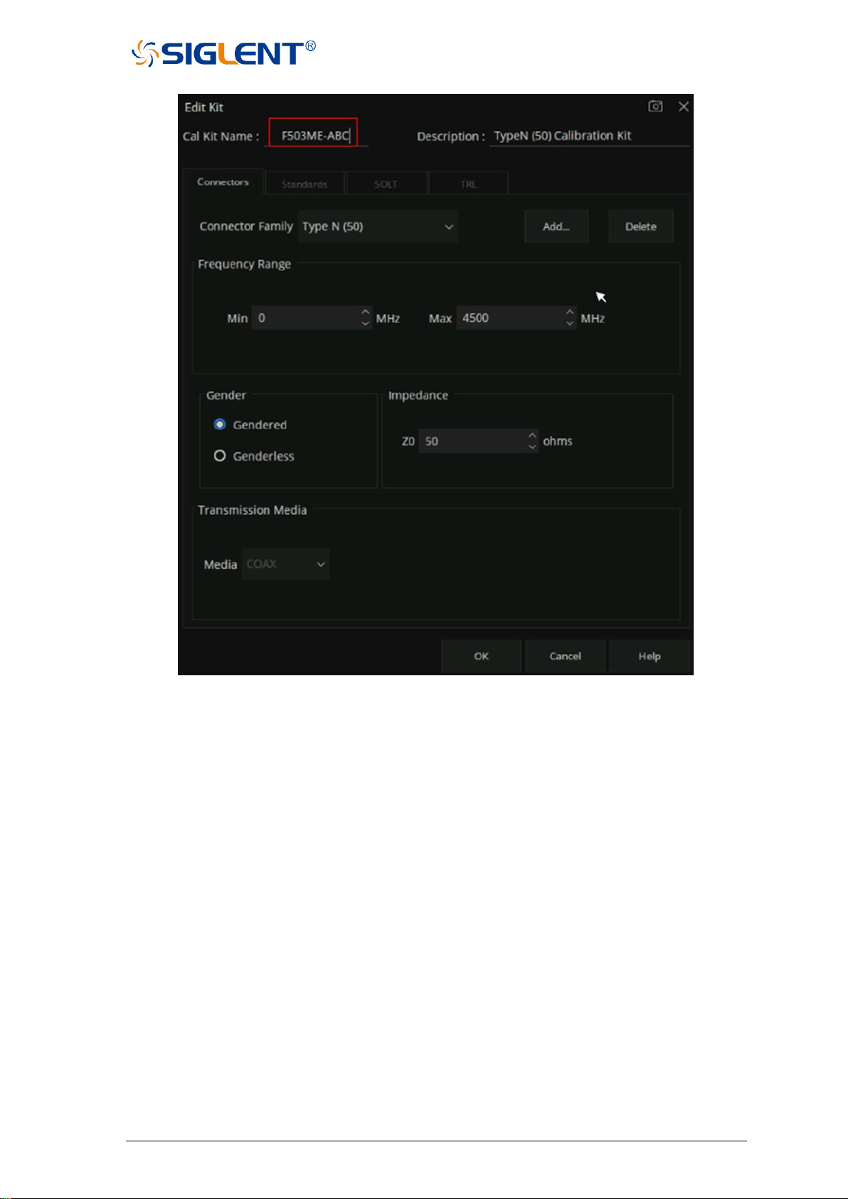
SNA5000A Vector Network Analyzer User Manual 66
Figure 3-15 Edit the new import ECal Kit
4. Click the Connectors, Standards, SOLT, and TRL Tabs to modify the corresponding
parameters as you need.
5. Click “OK” for the changed Cal Kit to take effect.
Method 2:Create a custom Cal Kit directly for new connector types.
1. Press” Cal” > Cal > Cal Kit > Insert...
2. Enter the name and description of the custom Cal Kit.
3. Refer to Method 1, click the Connectors, Standards, SOLT, TRL tab to modify the
corresponding parameters.
4. Click "OK" to make the created calibration effective.

67 SNA5000A Vector Network Analyzer User Manual
Figure 3-16 View the newly created Cal Kit
3.3.2 S Parameter calibration wizard
S parameter user calibration can be started after selecting the required S parameter
calibration type in the calibration wizard and setting the corresponding parameters.
Operating instructions:
Press the Cal key, use the knob or the arrow key to make the focus fall on Basic Cal, and
press Enter to enter the setting interface of the calibration kit:
Figure 3-17 Calibration wizard interface
Select the number of ports to be calibrated from the port menu in the calibration wizard
interface, and select the corresponding calibration kit model in the Cal Kit pull-down option.
Select the gender properties of the calibration connector from the DUT Connector drop-down
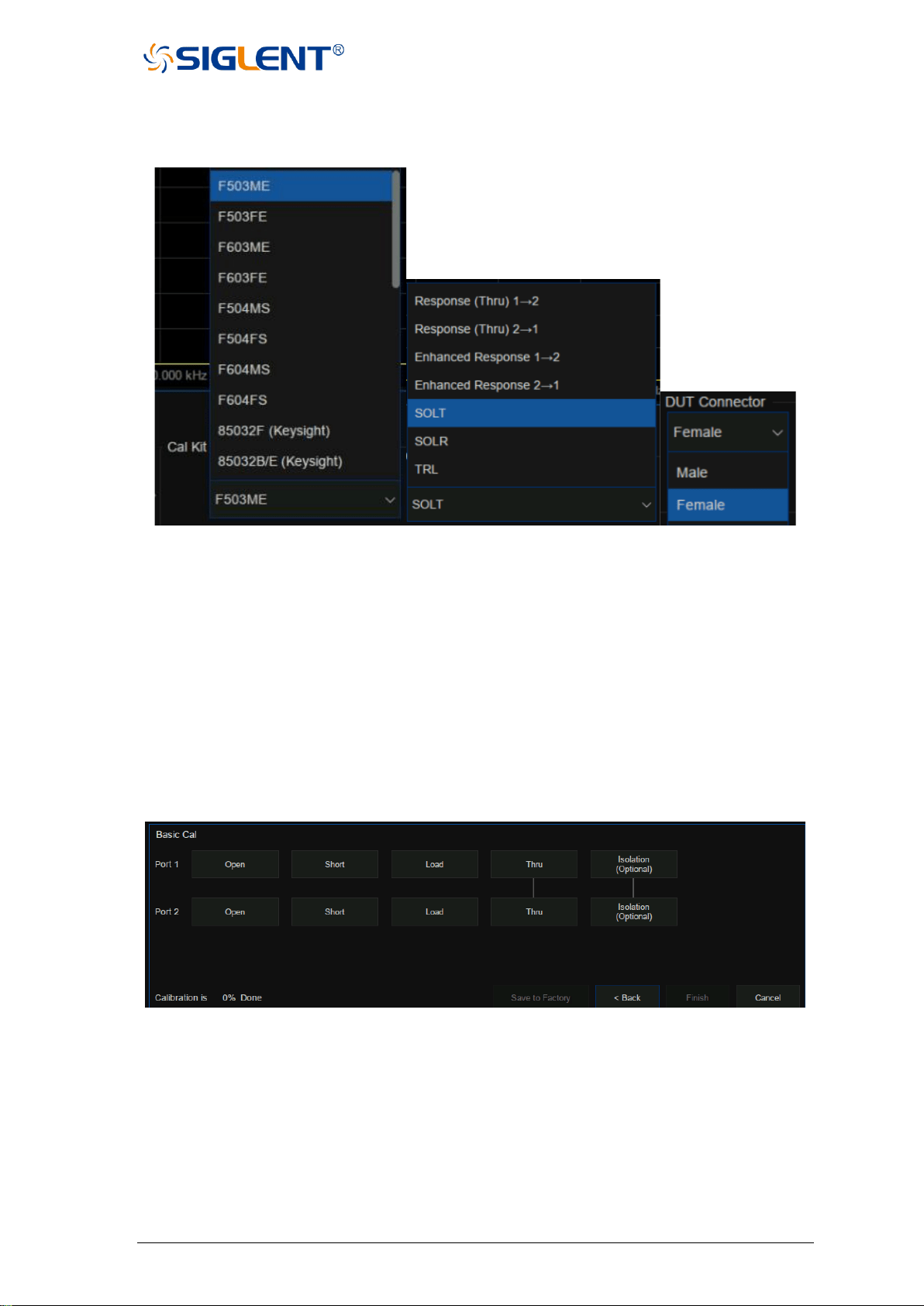
SNA5000A Vector Network Analyzer User Manual 68
option, and select the corresponding calibration method from the Cal Type drop-down option,
as shown in the figure below:
Figure 3-18 Calibration wizard interface
After the calibration is set, a specific calibration item interface will appear as shown in the
figure below. Here, taking the two-port SOLT calibration method as an example, it includes
several calibration items: OPEN, SHORT, LOAD, THRU, ISOLATION, among which the
ISOLATION calibration item may not be calibrated. There is no sequence relation between
these calibration terms. Simply select the corresponding calibration kit and click the
corresponding calibration item menu on the interface.
After completion of the corresponding calibration item, the percentage of calibration
progress will be displayed in the lower-left corner of the interface. When all the calibration
steps are completed, the calibration progress bar will show 100%. Click Finish to exit the
calibration interface, calibration results are automatically loaded in the current screen.
Figure 3-19 Calibration wizard interface
To Save the current calibration data for future use, press the Save Recall button and use
the knob or arrow keys to bring the focus to the Save State menu bar. Select State+Cal Data
from the Save Type drop-down option, click Save State As and enter the file name, and click
OK to Save the current calibration Data and the current setting State.
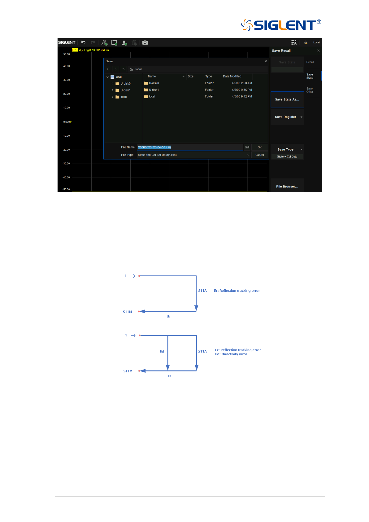
69 SNA5000A Vector Network Analyzer User Manual
Figure 3-20 Calibration wizard interface
3.3.3 Open Response Calibration
When a single port is used for open-circuit response calibration, the reflection tracking error
in the error model of the test device can be calculated by only connecting the OPEN calibration
element to the test port. If the LOAD calibration element is used for isolation calibration at the
same time, the directional error can be calculated.
Figure 3-21 Schematic diagram
Operating steps:
1. Preset vector network analyzer.
2. Set internal source output power, IF bandwidth, scan points, test frequency band and other
parameters.
3. Select Cal→Basic Cal to enter the Settings screen.
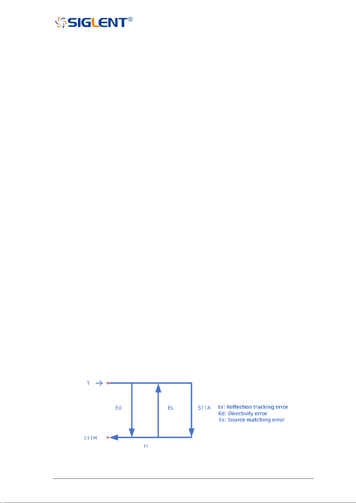
SNA5000A Vector Network Analyzer User Manual 70
4. Select only Port1 or Port2, select the required calibration kit in the Cal Kit, select the Type
of calibration element connector, Female or Male, in the DUT Connector, select
Response(Open) in the Cal Type, and click Next to proceed to the next step.
5. Connect the OPEN calibration element to the test port according to the interface prompts,
click Open for calibration, and click Finish to exit the calibration interface after calibration,
complete the calibration, and save the calibration data.
3.3.4 Short circuit response calibration
Like the open-circuit response calibration, the single-port short-circuit response is
connected to the port with the SHORT calibration element, and the reflection tracking error can
be calculated. If the LOAD calibration element is used for isolation calibration at the same time,
the directional error can also be calculated.
Operating steps:
1. Preset Vector network analyzer.
2. Set internal source output power, IF bandwidth, scan points, test frequency band and other
parameters.
3. Select Cal→Basic Cal to enter the setting interface.
4. Select only Port1 or Port2, select the required calibration kit in the Cal Kit, select the Type
of connector, Female or Male, in the DUT Connector, select Response(Short) in the Cal
Type, and click Next to proceed to the next step.
5. Connect the Short calibration element to the test port according to the interface prompts,
click Short for calibration, and click Finish to exit the calibration interface, complete the
calibration, and save the calibration data.
3.3.5 Full 1 port OSL calibration
All 1-port OSL calibration connects the OPEN, SHORT, and LOAD calibration elements to
the test ports in turn to calculate the reflection tracking error, directional error, and source
matching error in the error model of the test device.
Figure 3-22 Schematic diagram
Operating steps:
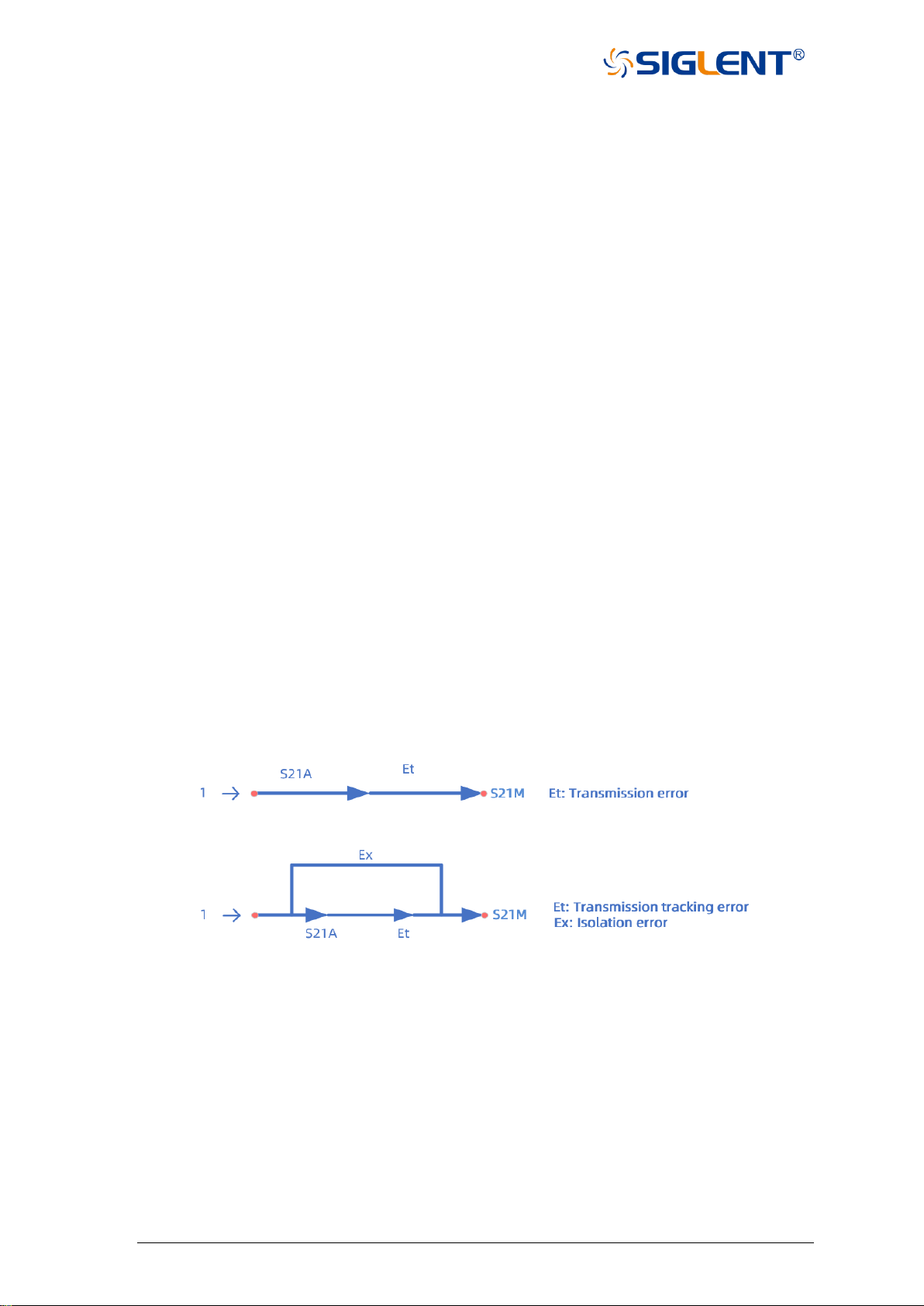
71 SNA5000A Vector Network Analyzer User Manual
1. Preset Vector network analyzer.
2. Set internal source output power, IF bandwidth, scan points, test frequency band, and other
parameters.
3. Select Cal→Basic Cal to enter the setting interface.
4. Select only Port1 or Port2, select the desired calibration kit in the Cal Kit, select the Type
of calibration connector, Female or Male, in the DUT Connector, select
OSL (Open, Short, Load) in the Cal Type, and click Next to proceed to the next step.
• Connect the OPEN calibration element to the test port according to the interface
prompts:
• Click Open for calibration
• Then connect the SHORT calibration element to the test port, click Short for
Calibration.
• Finally, connect the LOAD calibration element to the test port, click the Load for
Calibration.
• After the calibration, click Finish to exit the calibration interface, complete the
calibration, and save the calibration data.
3.3.6 Transmission response calibration (two ports)
Two-port transmission response calibration is to connect the THRU calibration kit between
two ports to calculate the transmission tracking error in the test device error model. If the LOAD
calibration kit is used for isolation calibration at the same time, isolation error (crosstalk error)
can also be calculated.
Figure 3-23 Schematic diagram
Operating steps:
1. Preset Vector network analyzer.
2. Set internal source output power, IF bandwidth, scan points, test frequency band, and other
parameters.
3. Select Cal→Basic Cal to enter the setting interface.
4. Select both Port1 and Port2, select the desired calibration kit in the Cal Kit, select the Type

SNA5000A Vector Network Analyzer User Manual 72
of calibration connector, Female or Male, in the DUT Connector, Select Response (Thru)
1→2 or Response(Thru) 2→1 in the Cal Type (the difference is to test S21 or S12), and
click Next to proceed to the next step.
5. Connect the Thru calibration element between the test ports according to the interface
prompts, click Thru for calibration, and click Finish to exit the calibration interface, complete
the calibration, and save the calibration data.
3.3.7 Enhanced response calibration (two ports)
Two-port enhanced response calibration connects the Thru calibration element between two
ports, and only connects the Open, Short, and Load on one port for calibration, or connects
the LOAD element to both ports for isolation calibration.
Operating steps:
1. Preset Vector network analyzer.
2. Set internal source output power, IF bandwidth, scan points, test frequency band, and other
parameters.
3. Select Cal→Basic Cal to enter the setting interface.
4. Select both Port 1 and Port 2, select the desired calibration kit in the Cal Kit, select the type
of calibration connector, Female or Male, in the DUT Connector, Select Enhanced
Response 1→2 or Enhanced Response(Thru) 2→1 in the Cal Type (the difference is that
S21 or S12 is tested during THRU calibration), and click Next to proceed to the next step.
5. According to the interface prompts, connect Open, Short, and Load on a test port to complete
the calibration successively, and then connect the THRU calibration kit between the two
ports to perform the Thru calibration. After the calibration is completed, click Finish to exit
the calibration interface, complete the calibration and save the calibration data.
3.3.8 SOLT calibration (two ports)
Two-port SOLT calibration connects the Open, Short, and Load calibration elements to each
test port in turn and the THRU calibration kit between the two test ports. All 12 error parameters
of the two ports can be calculated, including 6 forward and 6 reverse errors, including
directional, source matching, reflection tracking, transmission tracking, isolation (crosstalk),
and load matching errors. It is also possible to connect the LOAD element to both ports for
isolation calibration.
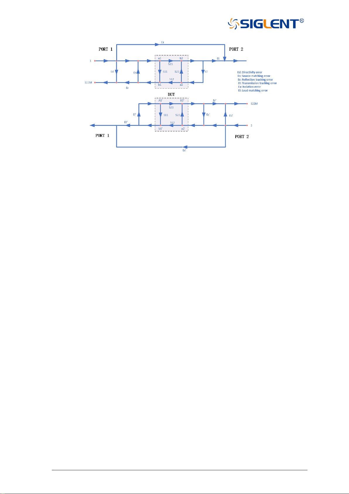
73 SNA5000A Vector Network Analyzer User Manual
Figure 3-24 Error model diagram
Operating steps:
1. Preset vector network analyzer.
2. Set internal source output power, IF bandwidth, scan points, test frequency band, and other
parameters.
3. Select Cal→Basic Cal to enter the Settings screen.
4. Select both Port 1 and Port 2, select the desired calibration kit in the Cal Kit, select the
type of calibration connector, Female or Male, in the DUT Connector, select SOLT in the
Cal Type, and click Next to proceed to the next step.
4. According to the interface prompts, connect the Open, Short, and Load calibration
elements to Port 1 successively, and click the corresponding Open, Short, and Load
items successively to complete the Port 1 calibration.
6. According to the interface prompts, connect the Open, Short, and Load calibration elements
to Port2 successively, and click the corresponding Open, Short, and Load items
successively to complete the Port 2 calibration.
7. According to the interface prompts, connect the THRU calibration kit between the two ports
to perform the Thru calibration.
8. After the calibration, click Finish to exit the calibration interface, complete the calibration,
and save the calibration data.
3.3.9 SOLR unknown through calibration (two ports)
In contrast to the two-port SOLT calibration, the error term in the test unit can be calculated
without knowing the S-parameter of the THRU straight-through calibration. The calibration
method is similar to that of SOLT in that it is possible to connect the LOAD to both ports for
isolated calibration.

SNA5000A Vector Network Analyzer User Manual 74
Operating steps:
1. Preset vector network analyzer.
2. Set internal source output power, IF bandwidth, scan points, test frequency band, and other
parameters.
3. Select Cal→Basic Cal to enter the Settings screen.
4. Select both Port 1 and Port 2, select the desired calibration kit in the Cal Kit, select the
Type of calibration Connector, Female or Male, in the DUT Connector, select SOLR in
the Cal Type, and click Next to proceed to the next step.
5. According to the interface prompts, connect the Open, Short, and Load calibration
elements to Port 1 successively, and click the corresponding Open, Short, and Load
items successively to complete the Port 1 calibration.
6. According to the interface prompts, connect the Open, Short, and Load calibration
elements to Port 2 successively, and click the corresponding Open, Short, and Load
items successively to complete the Port 2 calibration.
7. Connect the THRU calibration kit between the two ports according to the interface prompts.
The parameters of the THRU do not have to be known. Carry out unknown through Thru
calibration.
8. After the calibration, click Finish to exit the calibration interface, complete the calibration,
and save the calibration data.
3.3.10 TRL Direct Reflection Transmission Line Calibration (Two
Ports)
The two-port TRL calibration method does not need to know the index parameters of the
calibration kit, and all the error items in the error model of the test device can be figured out
through three simple connection methods. TRL calibration scheme will use the THRU straight
through calibration element, reflection calibration kit (Open or Short), and a small section of
transmission line.
Operating steps:
1. Preset vector network analyzer.
2. Set internal source output power, IF bandwidth, scan points, test frequency band, and other
parameters.
3. Select Cal→Basic Cal to enter the Settings screen.
4. Select both Port 1 and Port 2, select the desired calibration kit in the Cal Kit, select the
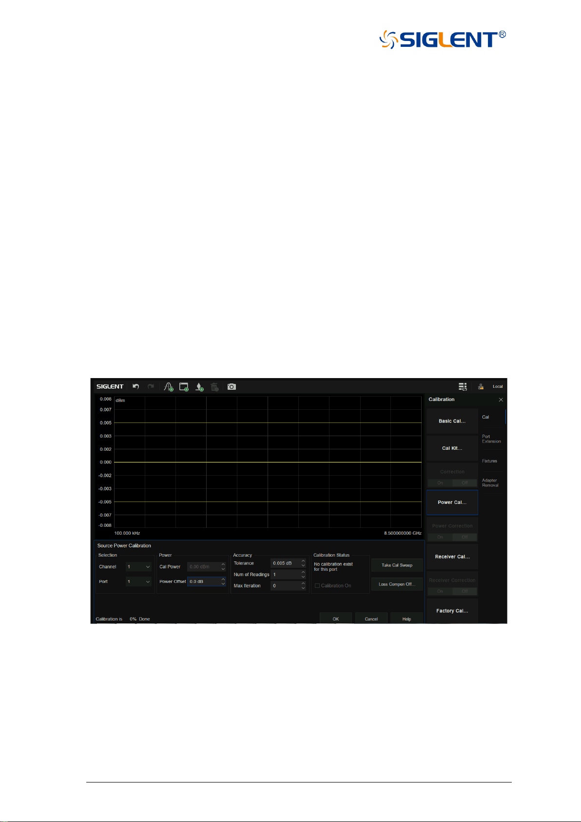
75 SNA5000A Vector Network Analyzer User Manual
Type of calibration kit Connector, Female or Male, in the DUT Connector, select TRL in
the Cal Type, and click Next to proceed to the next step.
5. According to the interface prompts, connect the THRU calibration kit, Reflect (Open or
Short) calibration element, and Line on a Port 1 in turn, and click the corresponding Thru,
Reflect, and Line items in turn to complete the Port 1 calibration.
6. According to the interface prompts, connect the THRU calibration element, Reflect (Open
or Short) calibration element, and transmission line on a Port 2 in turn, and click the
corresponding Thru, Reflect, and Line items to complete the Port 2 calibration.
7. After the calibration, click Finish to exit the calibration interface, complete the calibration,
and save the calibration data.
3.4 Internal source power calibration
The vector network analyzer has been calibrated for the output power of the transmitter
before it leaves the factory, but the factory calibration may not guarantee sufficient accuracy in
all cases. To improve the accuracy, the user can conduct an internal source power calibration
before performing any tests.
Figure 3-25 Transmitter power calibration
Before attempting power calibration, power loss compensation at different frequency points
can be set as shown in the figure below. Click "+" successively to add corresponding frequency
and loss values. After setting, click OK to save the data.
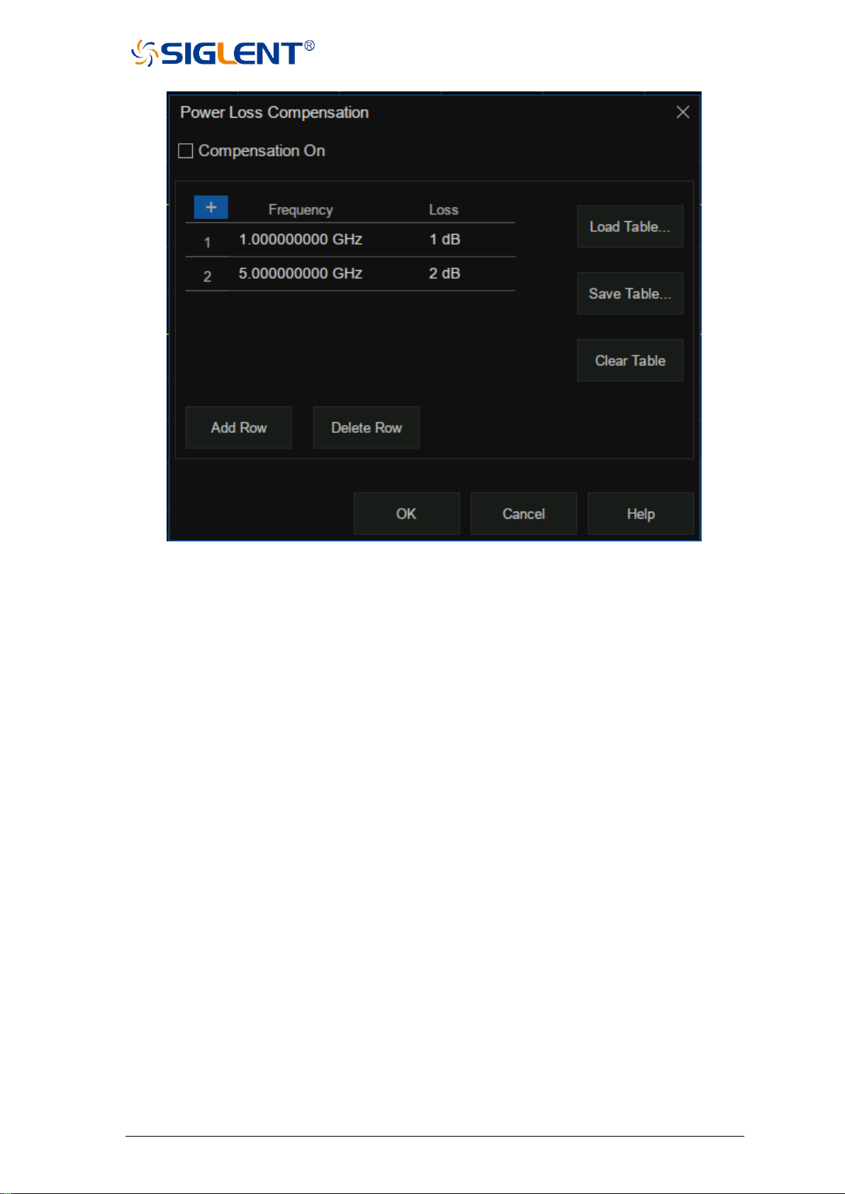
SNA5000A Vector Network Analyzer User Manual 76
Figure 3-26 Set the interface
Power calibration operation steps:
1. Connect the port-under-test to a compatible power meter (Keysight U2000 series, R&S
NRP series, etc..) and probe to ensure normal communication between the vector
network analyzer and the power meter.
2. Preset vector network analyzer.
3. Set internal source output power, IF bandwidth, scan points, test frequency band and other
parameters.
4. Select Cal→Power Cal to enter the Settings screen.
5. Select the test channel and select the power output port.
6. Set parameters such as power offset, capacity limit, reading times, maximum iteration
times, etc.
7. Click Take Cal Sweep to start the power output measurement.
8. Click OK to complete the calibration and exit the power calibration interface after the
measurement is completed.
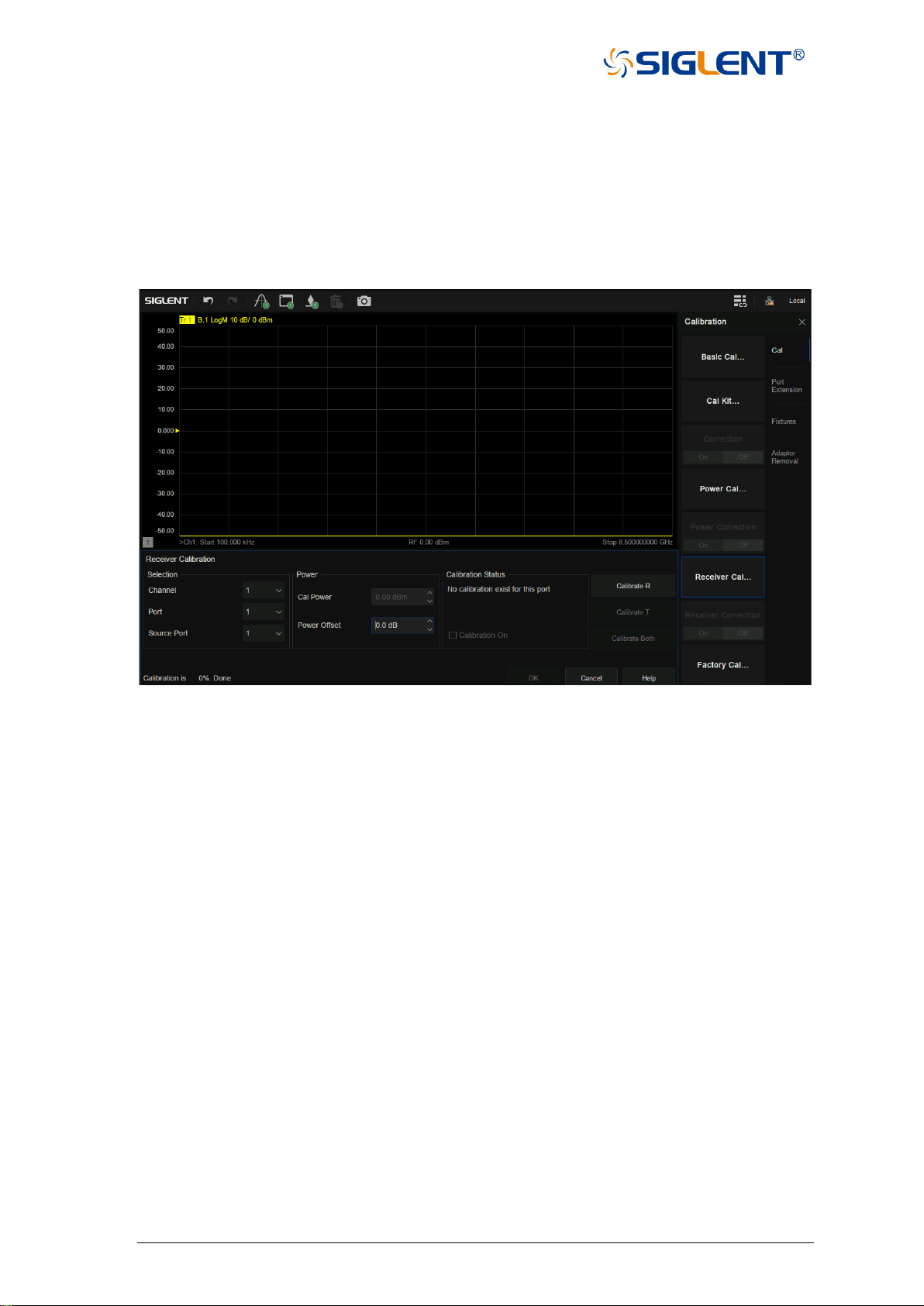
77 SNA5000A Vector Network Analyzer User Manual
3.5 Receiver calibration
The vector network analyzer receiver power has been factory calibrated, but the factory
calibration may not guarantee sufficient accuracy in every situation. The user can conduct a
receiver power calibration before the test to improve the test accuracy. To ensure the
calibration accuracy of the receiver, it is better to calibrate the power of the internal source
before the calibration of the receiver.
Figure 3-27 Receiver calibration setting interface
Operating steps:
1. Preset vector network analyzer.
2. Set internal source output power, IF bandwidth, scan points, test frequency band, and other
parameters.
3. Select Cal→Receiver Cal to enter the Settings screen.
4. Select the test channel, select the internal source output port, select the receiver port
5. Connect the two ports using an appropriate specification RF cable.
6. Set parameters such as power offset.
7. Calibrate R or Calibrate T or Calibrate Both can be clicked to begin receiver calibration.
8. Click OK to complete the calibration and exit the receiver calibration interface.
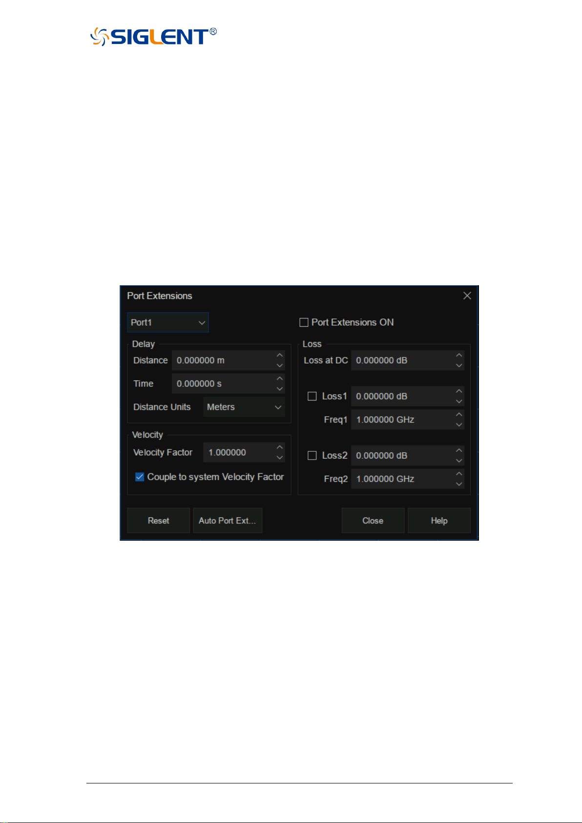
SNA5000A Vector Network Analyzer User Manual 78
3.6 Port extension
Eliminating the errors of test fixturing can be a difficult task. The port extension function of
a vector network analyzer is a good method to eliminate the error of test fixtures. The
calibration of S parameters is usually carried out by the user at the plane where the RF cable
is connected to the test fixture, typically a connector (SMA, N-type, etc..). The actual device
to be tested is located in the test fixture. The device to be tested and the test fixture are
generally connected by a microstrip line. As a result, the actual measurement plane of the
device to be tested does not coincide with the calibration reference plane (the connector, as
mentioned previously) which will introduce calibration errors.
After the S parameter calibration is performed, the reference plane can be extended to
the specified measurement plane by simply adding the added microstrip line length, speed
factor, loss, and other parameters in the setting interface, to carry out more accurate testing.
Figure 3-28 Port extension setting interface
Manual port extension operation steps:
1. Perform the appropriate calibration type (SOLT, etc..) on the associated cabling before
entering Port Extensions.
2. Select Cal→Port Extension→Port Extension to enter the Settings screen.
3. Select the port that needs to be extended, the unit of length, and input the velocity
coefficient.
The velocity coefficient is different, and the propagation time of electromagnetic waves on
the transmission line is different. Input the length of the extended transmission line and
the time will be calculated automatically.

79 SNA5000A Vector Network Analyzer User Manual
If the transmission line has loss, the loss of the transmission line can be added, including
DC and AC loss.
The AC loss can be selected as LOSS1 at the single-frequency point or LOSS1 and
LOSS2 at the dual-frequency point.
Among them, the fitting algorithm for two forms of AC loss are:
Single-frequency point loss Loss1:
Loss(f) = Loss1 * (f/Freq1) ^ 0.5
Dual-frequency point loss Loss1,Loss2:
Set the low frequency point to LOSS1 and the high frequency point to LOSS2,
Loss(f) = Loss1 * (f/Freq1) ^ n, n = lg [abs(Loss1/Loss2)] / lg (Freq1/Freq2).
4. Select whether to coupling to the system speed factor. If unchecked, the speed factor is set
only for the specified port, and when checked, for all ports.
5. Check the Port Extensions ON button and the Port extension will take effect.
Manual port extensions require the user to manually enter the parameters of the extended
transmission line, while automatic port extension does not require prior knowledge of the
transmission line parameters. The calibration plane can be automatically extended to the
actual reference plane by simply performing an open or short circuit calibration on the actual
reference plane of the DUT. The automatic port extension function is not available in the
following cases:
1. The scan type is set to power scan.
2. The frequency offset is set to on.
3. Waveguide transmission line port extension.
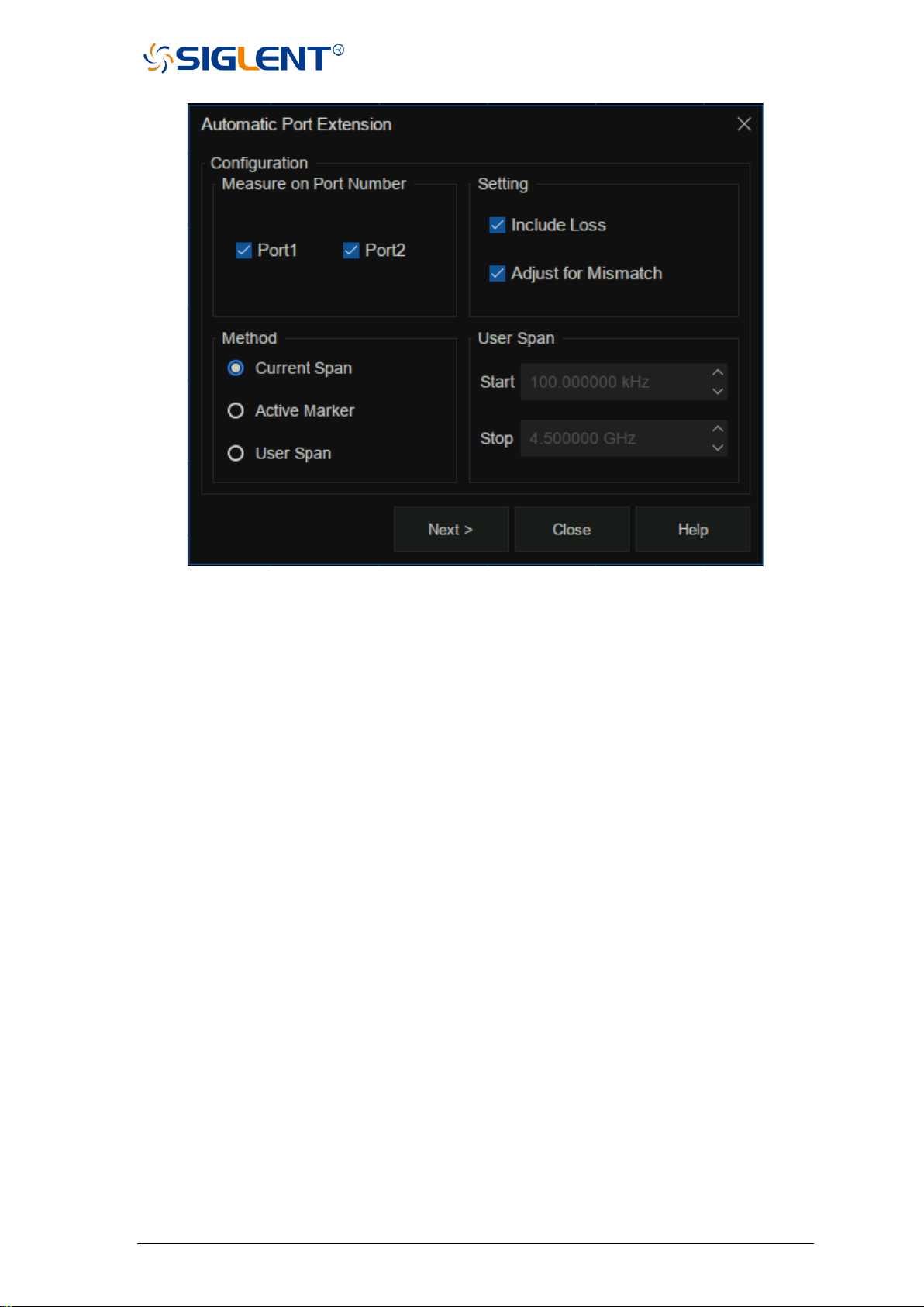
SNA5000A Vector Network Analyzer User Manual 80
Figure 3-29 Automatic port extension setting interface
Automatic port extension operation steps:
1. Perform the appropriate calibration type (SOLT, etc..) on the associated cabling before
entering Port Extensions.
2. Select Cal→Port Extension→Auto Port Extension to enter the Settings screen.
3. Select the port you want to extend. Refer to practical application scenarios, select Port 1
or Port 2, or both ports.
4. Select the frequency span of the test.
There are three frequency spans to choose:
Current Span: The frequency span of the current interface setting.
Active Marker: The frequency point currently marked, In this case, Loss2 can be ignored
when +setting loss, only Loss1 can be set.
User Span: Use the start and end frequencies set by the user.
5. Set whether the loss should be included or not. Select this box to automatically measure the
loss in the transmission line and apply it to the calibration.
6. The mismatch adjustment option is only available when the inclusion loss item is selected.
The mismatch increases the ripple on the trace lines of S11 and S22. If the ripple is large,
the trace display of S11 and S22 will be greater than 0 dB, resulting in unstable values when
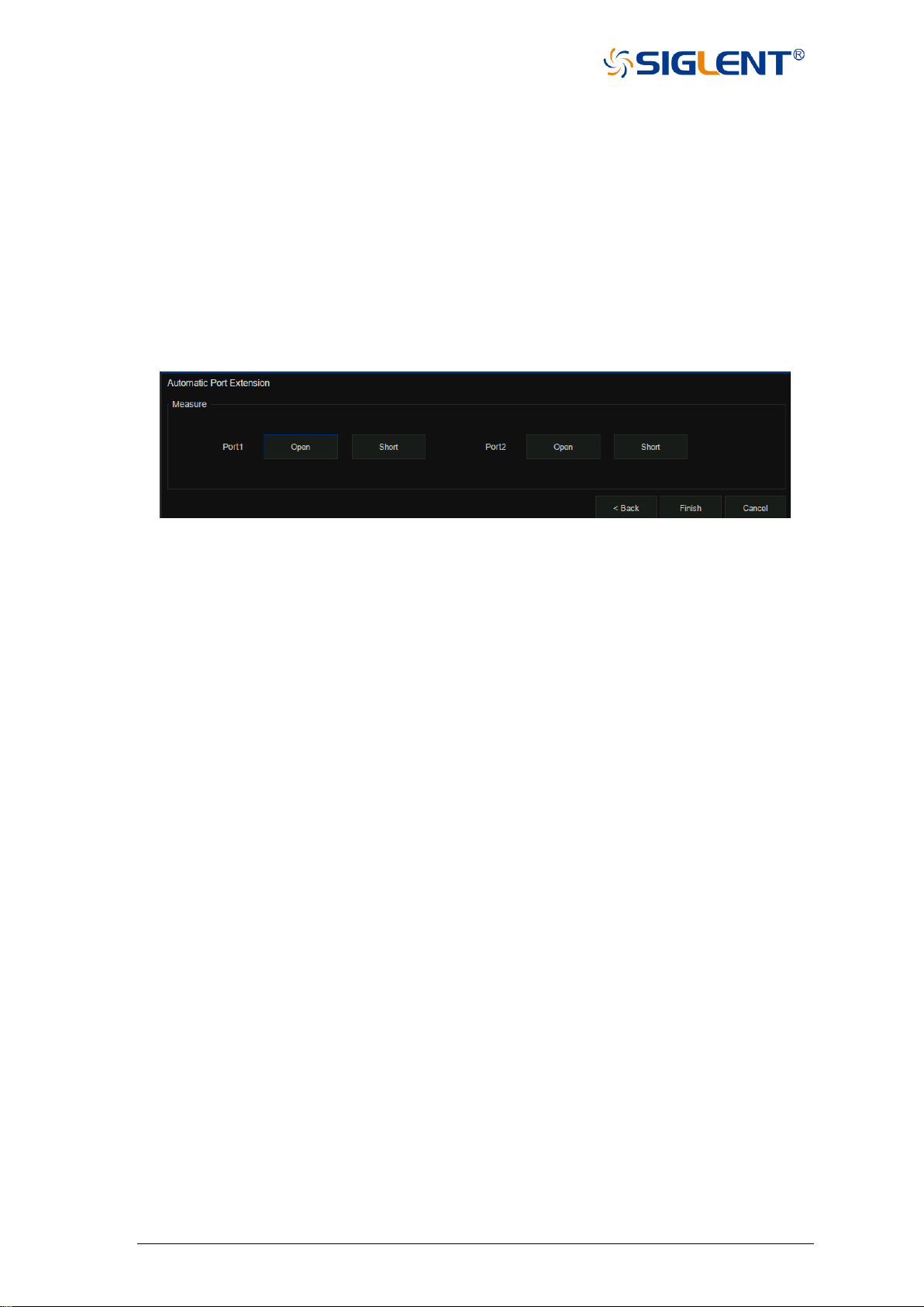
81 SNA5000A Vector Network Analyzer User Manual
S parameters are used. Selecting the adjustment mismatch item can increase the loss of the
fixture so that the peak value of the ripple is below 0 dB. Although this will increase the error,
it can prevent the numerical instability of S parameters from appearing when it is used.
7. Click Next to enter the measurement interface. Before the measurement, make sure that
the device has been removed from the test fixture. In this way, the open-circuit
measurement can be performed. Of course, the test fixture can also refer to the plane Short
circuit to conduct the Short measurement. It can carry out one of the Open or Short
measurements or simultaneously carry out the Open and Short measurements. When two
measurements are used, the result will be the average of the two measurements, and the
accuracy will be improved.
Figure 3-30 Automatic port extension calibration interface
3.7 Fixture measurement function
In addition to the port extension function, the vector network analyzer also provides several
other functions for test fixtures:
1. Port match (2-port embedding)
2. Port impedance conversion
3. 2-port de-embedding
4. N port embed/de-embed (port 4/6/8)
5. Differential port match
6. Differential port impedance conversion
7. Common port impedance conversion
Port match operation steps:
1. Ensure that the user has completed the S parameter calibration and obtained the S
parameters of the DUT.
2. Select Cal→Fixtures→Fixture Setup→Port Match to enter the Settings screen.
3. By selecting the port and the parameter representation form of the matching module, the
S2P file (AKA Touchstone file) of the matching module can be directly exported or the
circuit model of the matching module can be used. It supports 9 topologies which are
combined by L, R, G, and C. It is necessary to manually set the parameter values of L, R,
G, and C components. Checking the Enable Port Matching On All Ports tab means that
all ports are matched. When the frequency range in the S2P file of the imported matching
module is less than the frequency range set by the current interface, such as the Enable
Extrapolation item is not checked, the system will extrapolate the S2P file by default. In
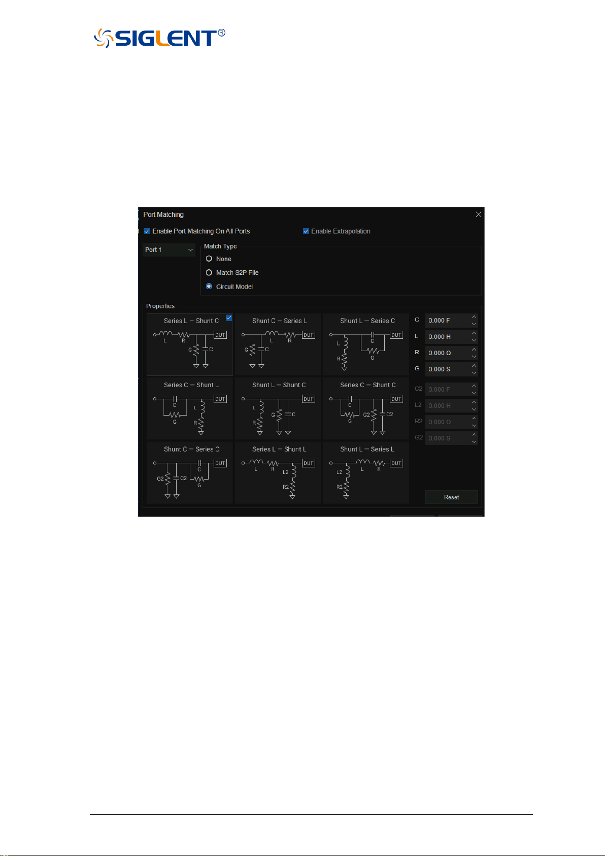
SNA5000A Vector Network Analyzer User Manual 82
other words, all the uncovered low-frequency parameters are replaced by the first point in
the S2P file and all the uncovered high-frequency parameters are replaced by the last
point in S2P file making the frequency range of the S2P file the same as the frequency
range of the current interface. If you check the Enable Extrapolation tab, the system will
interpolate the frequency points not covered by S2P so that the frequency range of the
S2P file is the same as that of the current interface.
4. Click Close to complete the setting and click Apply Fixtures to ON to take effect.
Figure 3-31 Port match
Port impedance conversion operation steps:
1. Ensure that the user has completed the S parameter calibration and obtained the S
parameters of the DUT.
2. Select Cal→Fixtures→Fixture Setup→Port Z to enter the Settings screen.
3. Choose the port, the default system port characteristic impedance is 50 Ω, you can fill in the
required resistance values in the R and JX columns, Then the S parameter displayed will be
automatically converted to the S parameter corresponding to the new characteristic
impedance. Checking the Enable Port Z Conversion On All Ports tab means port
matching is performed on all ports.
4. Click Close to complete the setting and click Apply Fixtures to ON to take effect.

83 SNA5000A Vector Network Analyzer User Manual
Figure 3-32-port impedance conversion
2-port de-embed operation steps:
1. Ensure that the user has completed the S parameter calibration and obtained the S
parameters of the DUT.
2. Select Cal→Fixtures→Fixture Setup→2-Port DeEmbed to enter the Settings screen.
3. Select the port and select the form of de-embedding to import an S2P File. Click User S2P
File to import the S parameter of the fixture part that needs to be removed.
Checking the Enable De-Embedding On All Ports tab means that all ports are de-
embeddable.
When the frequency range in the S2P file of the imported matching module is smaller than
the frequency range set by the current interface, if the Enable Extrapolation item is not
checked, the system will extrapolate the S2P file by default. All the low-frequency
parameters not covered are replaced by the first point in the S2P file, and all the high-
frequency parameters not covered are replaced by the last point in the S2P file, making the
frequency range of the S2P file the same as that of the current interface.
If you check the Enable Extrapolation tab, the system will interpolate the frequency points
not covered by the S2P so that the frequency range of the S2P file is the same as that of
the current interface.
4. Checking the Reverse Adapter Ports entry represents the part of the reverse connection
that will need to be de-embedding. By default, the system reverses the imported S2P file.
5. Click Close to complete the setting and click Apply Fixtures to ON to take effect.
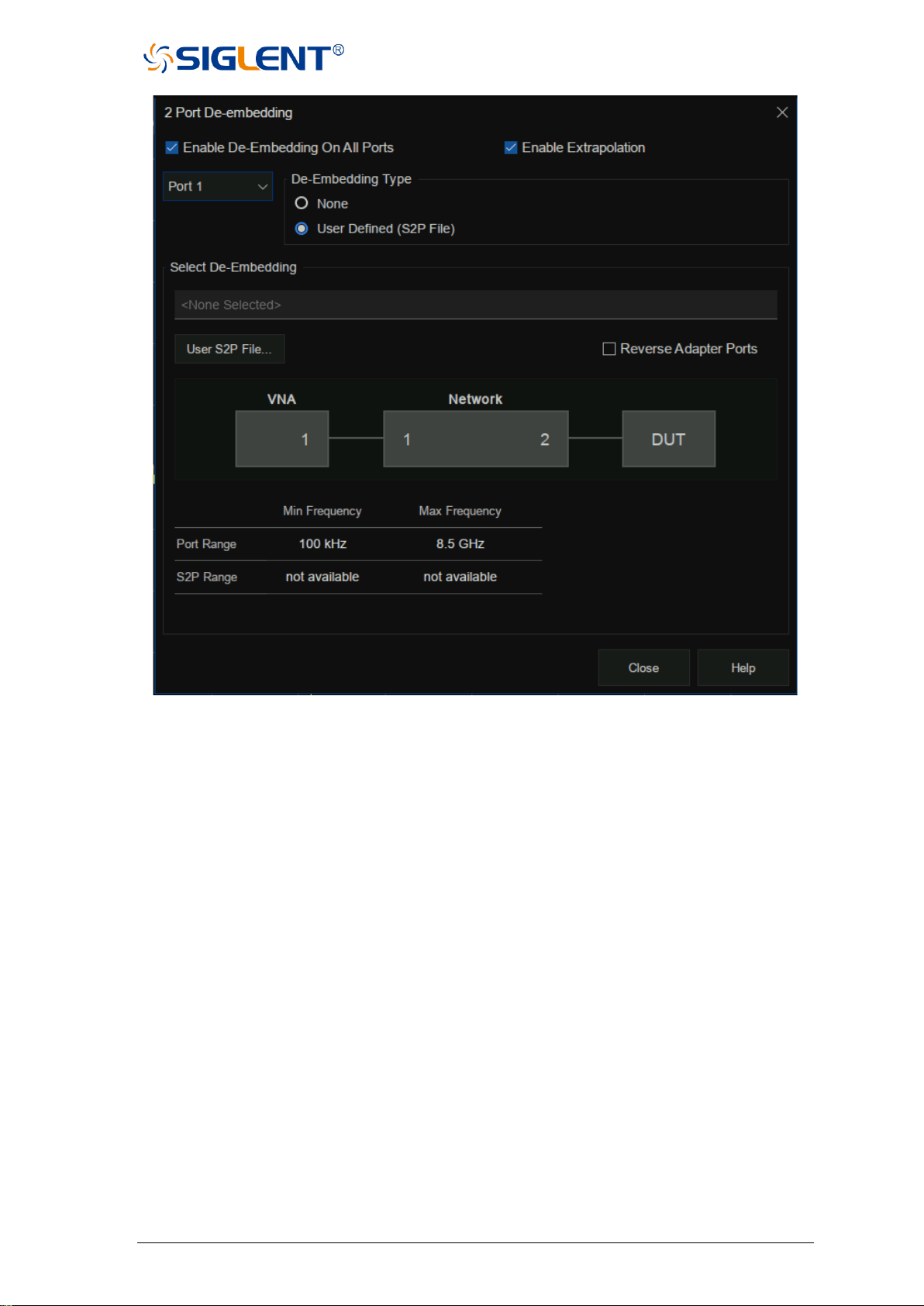
SNA5000A Vector Network Analyzer User Manual 84
Figure 3-33 de-embedding interface
N-port embedding/de-embedding operation steps:
1. Ensure that the user has completed the S parameter calibration and obtained the S
parameters of the DUT.
2. Select Cal→Fixtures→Fixture Setup→N-Port DeEmbed to enter the Settings screen.
3. Select the topology type.
There are 3 topology types:
A (using network 1)
B (using network 1 and 3)
C (using network 1, 2 and 4)
Select the port of the vector network analyzer in the VNA item, select the Network port
configuration that needs to be embedded or de-embedded in the Network, and select the
Embed operation or De-embed operation under each Network. Finally, load the S2P file
corresponding to the operating network. Checking the Enable 4/6/8-Port Embed/De-
embed On All Ports tab means that all ports are matched.
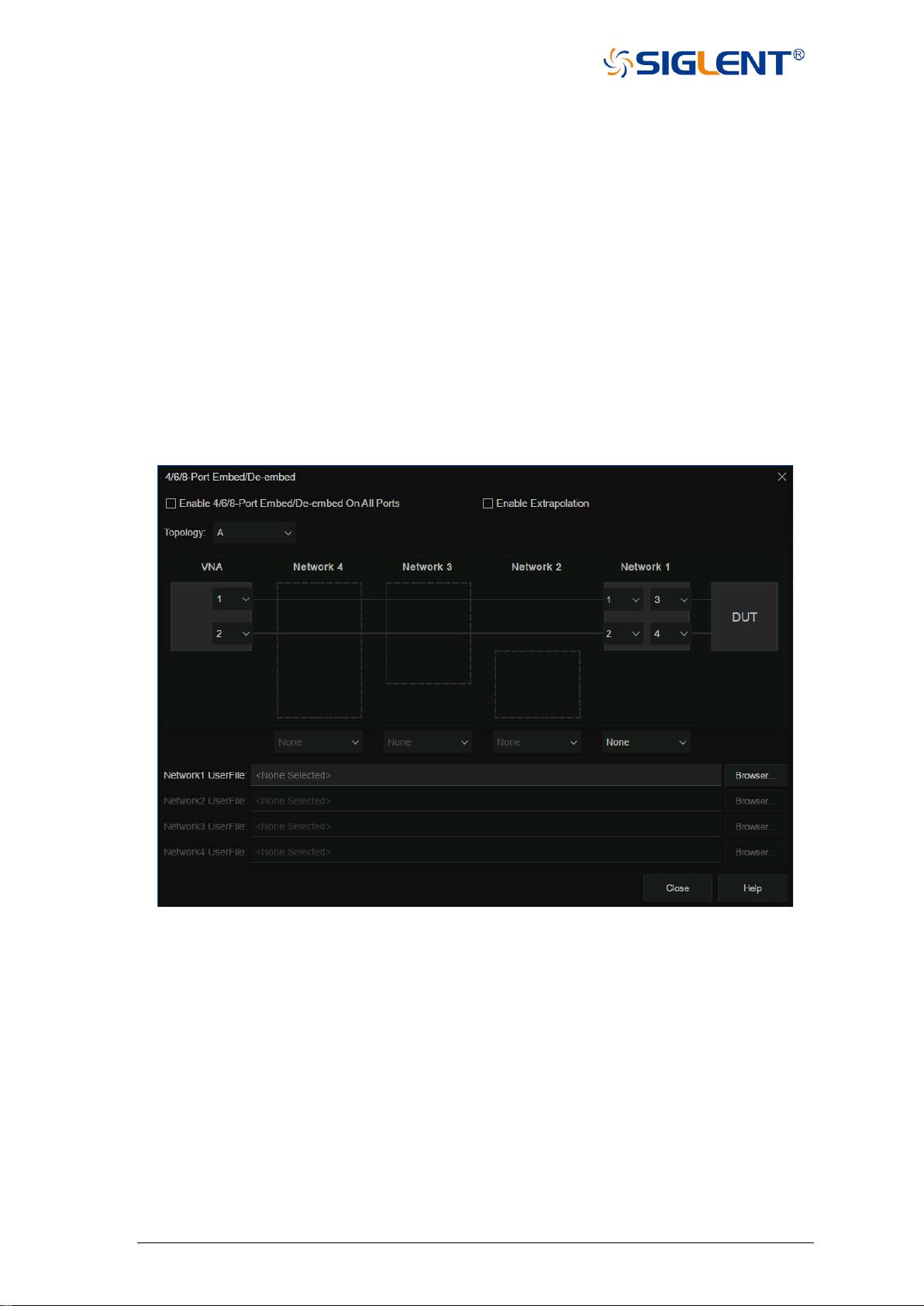
85 SNA5000A Vector Network Analyzer User Manual
When the frequency range in the S2P file of the imported matching module is less
than the frequency range set by the current interface, such as when the Enable
Extrapolation item is not checked, the system will extrapolate the S2P file by default.
In other words, all the uncovered low-frequency parameters are replaced by the first point
in the S2P file, and all the uncovered high-frequency parameters are replaced by the last
point in the S2P file, making the frequency range of the S2P file the same as the
frequency range of the current interface.
If you check the Enable Extrapolation tab, the system will interpolate the frequency
points not covered by S2P so that the frequency range of the S2P file is the same as that
of the current interface.
4. Click Close to complete the setting and click Apply Fixtures to ON to take effect.
Figure 3-34 De-embedding interface
Differential port match operation steps:
1. Ensure that the user has completed the S parameter calibration and obtained the balance
S parameters of the DUT.
2. Select Cal→Fixtures→Fixture Setup→Differential Port Match to enter the Settings
screen.
3. By selecting the port and the parameter representation form of the matching module, the
S2P file of the matching module can be directly imported or the circuit model of the
matching module can be used.
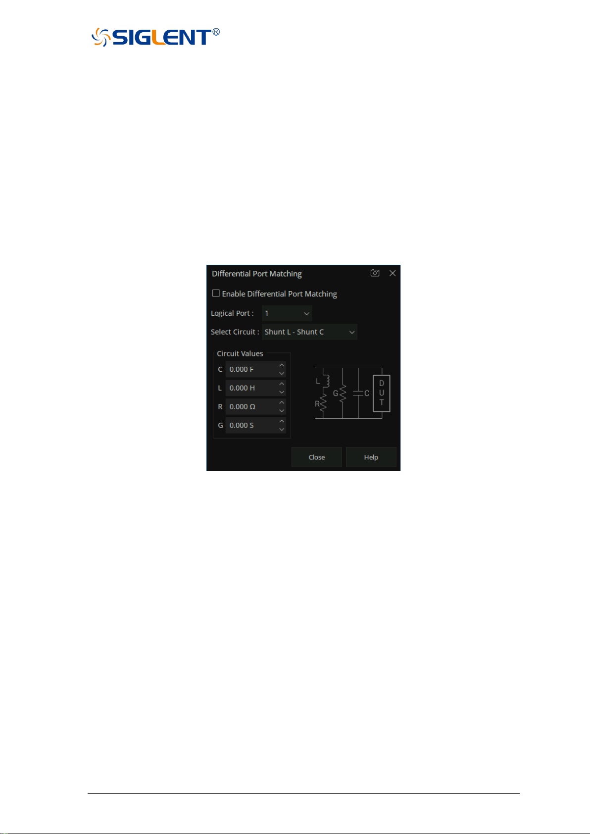
SNA5000A Vector Network Analyzer User Manual 86
It is necessary to manually set the parameter values of L, R, G, and C components if the
circuit model is used.
Checking the Enable Differential Port Matching tab means that all ports are matched.
When the frequency range in the S2P file of the imported matching module is less than
the frequency range set by the current interface, the system will extrapolate the S2P file
by default. In other words, all the uncovered low-frequency parameters are replaced by
the first point in the S2P file and all the uncovered high-frequency parameters are
replaced by the last point in the S2P file making the frequency range of the S2P file the
same as the frequency range of the current interface.
4. Click Close to complete the setting and click Apply Fixtures to ON to take effect.
Figure 3-35 Differential port match
Differential and common port impedance conversion operation steps:
The operation of differential port impedance conversion and common port impedance
conversion is similiar to that of port impedance conversion, please refer to the instructions of
the latter.
3.8 Adapter removal / insertion function
Adapters are often used when the network analyzer is used to test the DUT. The vector
network analyzer provides the function of removing and inserting adapters. Before the function
of removing and inserting adapters is enabled, the vector network analyzer needs to carry out
full 2-port calibration.
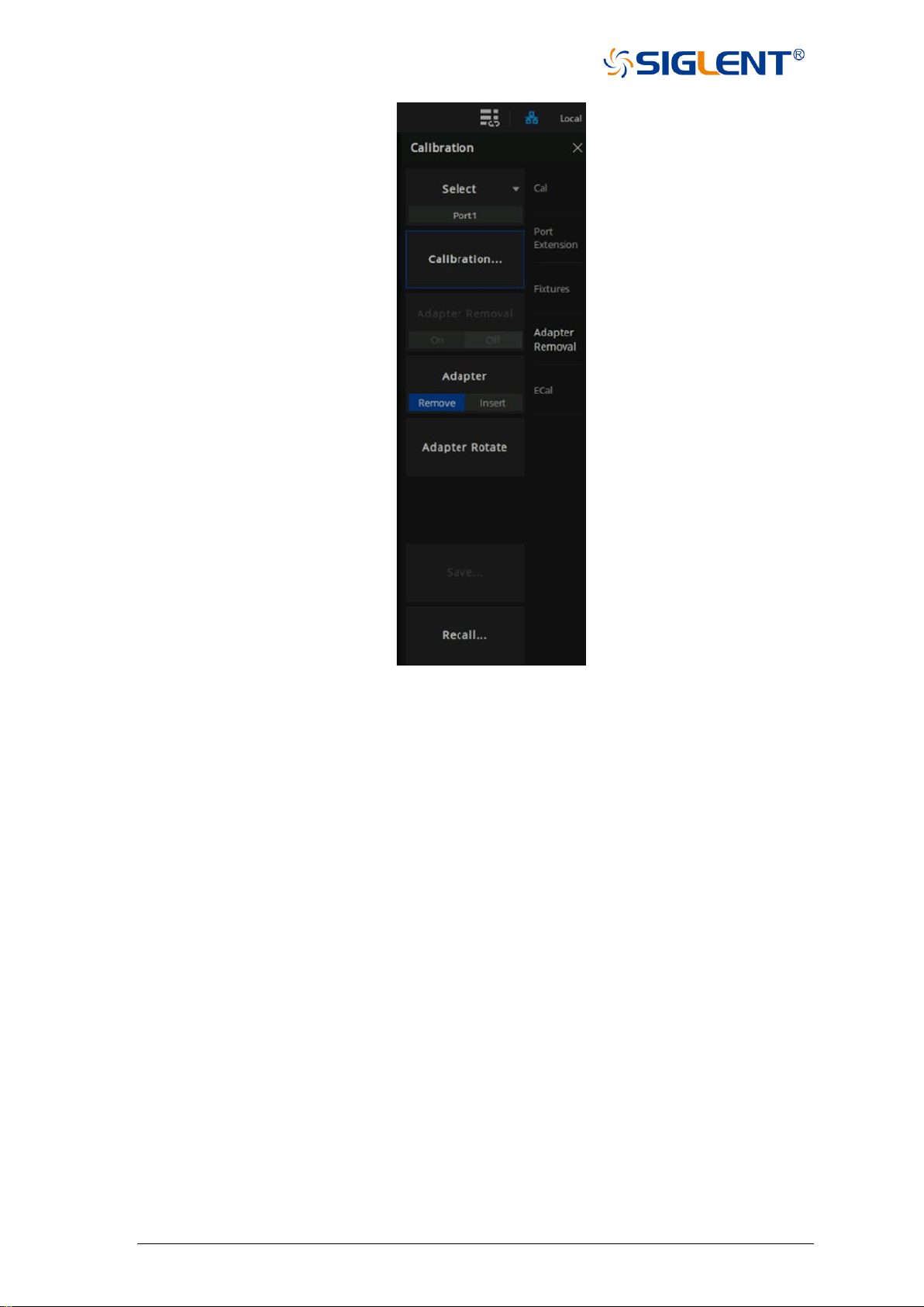
87 SNA5000A Vector Network Analyzer User Manual
Figure 3-36 Adapter removal and insertion functions
Adapter removal operation steps:
1. Connect the test cable of the vector network analyzer to the adapter, and configure the
parameters of the network analyzer. First, perform the full 2-port calibration.
2. Select Cal→Adapter Removal to go to the Settings screen and select Remove in the
Adapter tab.
3. Remove the adaptor from the test cable, Select Cal→Adapter Removal→Calibration to
enter the Adapter Removal configuration screen. Select the port connected to the adaptor
to be removed, select the calibration kit type, and select the polarity of the calibration kit.
Click Next to connect the Open, Short and Load calibration elements in turn for full 1 port
calibration.
4. Click Finish to complete the calibration and click Adapter Removal to ON to complete the
Adapter Removal operation.

SNA5000A Vector Network Analyzer User Manual 88
Figure 3-37 Adapter removal and insertion function calibration interface
Adapter insertion operation Steps:
1. Remove any test cables from the ports of the analyzer and perform a full 2-port calibration.
2. Select Cal→Adapter Removal to go to the Settings screen and select Insert in the
Adapter tab.
3. Connect the adapter on the test cable, select Cal→Adapter Removal→Calibration to
enter the Adapter Removal configuration screen. Select the port connected with the
adaptor to be inserted, select the calibration kit model, select the polarity of the calibration
kit, and click Next to connect the Open, Short, and Load calibration elements in turn for
full 1 port calibration.
4. Click Finish to complete the calibration and click Adapter Removal to ON to complete the
Adapter insertion operation.
“Adapter Rotate” is also known as the "equal exchange adapter and equal length adapter"
calibration method. Before the unknown pass-through method was introduced, the
switching adapter method was often used as a faster alternative to the more tedious
adapter removal method.
3.9 Ecal
3.9.1 ECal Overview
ECal is a new automatic calibration technology for vector network analyzers. Every ECal
module contains electronic standards that are automatically switched into position during a
measurement calibration. These electronic standards have been measured at the factory and
the data stored within the memory of the ECal module. The analyzer uses this stored data,
along with the measured data, to calculate the error terms for a measurement calibration. ECal
offers the following advantages:
⚫ The calibration process is simple. The electronic calibrator only needs to be connected to
the VNA once to complete the test items required by the dual-port calibration, without the
need for multiple calibration connections.
⚫ A shorter time is required for calibration.
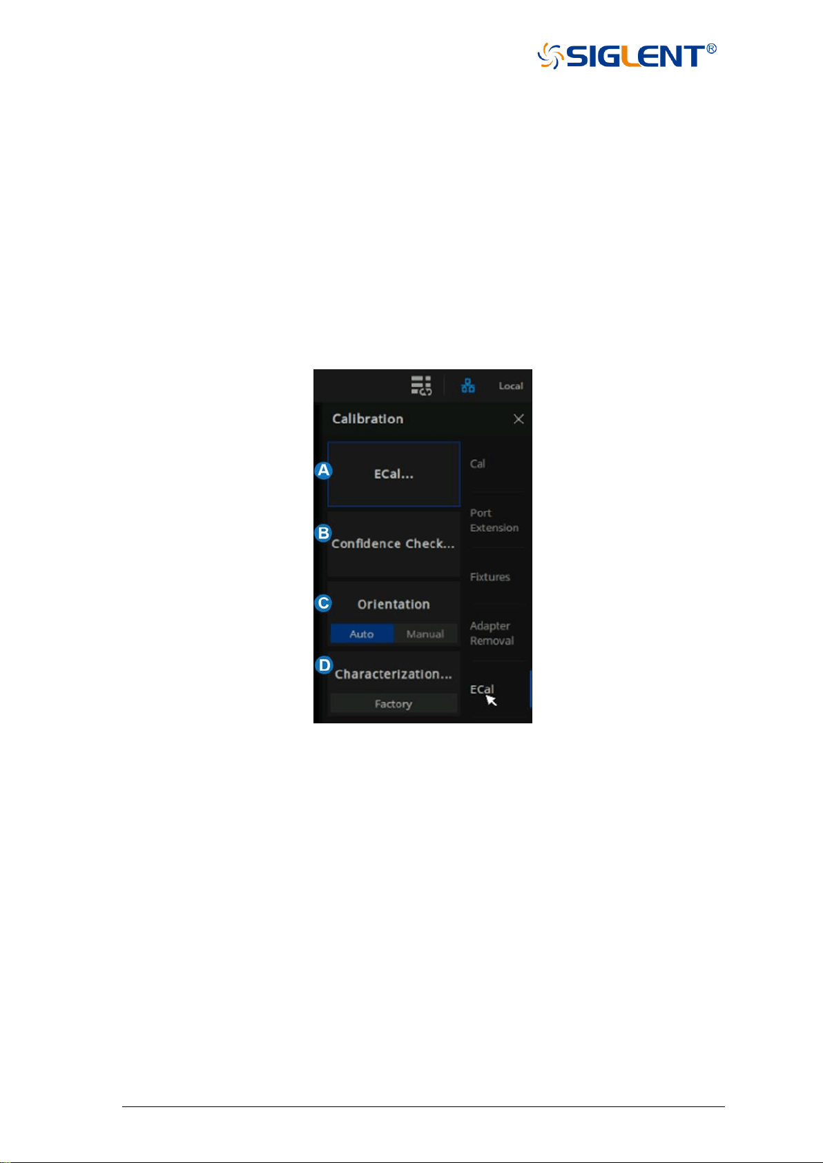
89 SNA5000A Vector Network Analyzer User Manual
⚫ There are fewer uncertain factors in the calibration process, and the probability of
electronic calibration being affected by misoperation is reduced because there is no need
for multiple connection processes.
Use ECal to perform calibration
1. Connect the USB port on the ECal module with the USB port on the front panel of VNA
via a USB cable. the module indicates “READY”. When you connect the module, the type
of module, frequency range, and connector type are automatically recognized.
2. Connect a port on the ECal module to the test port to be calibrated.
3. Press Cal > ECal on the front panel to enter the ECal menu interface.
Figure 3-38 ECal menu
A. ECal Config. Select the number of ports to calibrate. Then select the port number
configuration.
B. Confidence Check. Check the validity of Ecal calibration.
C. Orientation. Select ”Auto”(the default setting) the VNA automatically senses the model
and direction in which an ECal module port is connected to the VNA ports. Select
“Manual” to manually set the specified port.
D. Characterization. View the characterization information stored in the ECal module
3.9.2 ECal Config
Press “Cal “on the front panel , Press Cal > ECal > ECal to enter the menu interface of ECal
setting.
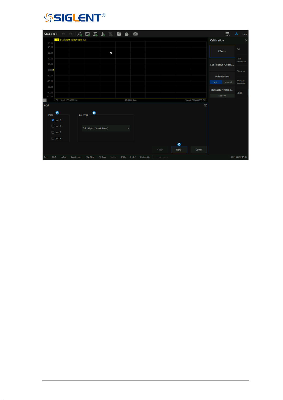
SNA5000A Vector Network Analyzer User Manual 90
Figure 3-39 ECal config menu
A. Select the number of ports to calibrate and configure the port number. Using ECal, you
can perform 1-Port Reflection calibration, Full 2-Port calibration, Full 3-Port calibration,
and Full 4-Port calibration.
B. Select the Cal Type.
C. When "Orientation" is Auto, click "Next" to enter the automatic alignment directly. When
"Orientation" is Manual, click "Next" to specify the calibration port and go to auto-
calibration.
3.9.3 Confidence Check
1. Press “Cal“ on the front panel, press Cal > ECal > Confidence Check to enter the menu
interface of Confidence Check.
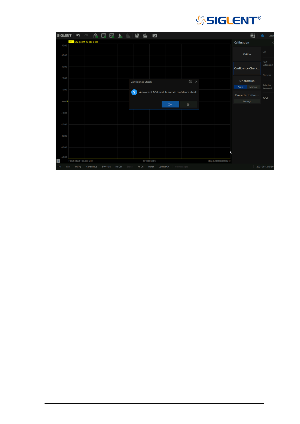
91 SNA5000A Vector Network Analyzer User Manual
Figure 3-40 Confidence Check
2. Compare the data-trace with the memory trace and verify that the measurement is correct.
3. The steps to compare when both data and memory traces are displayed are as below:
a) Press “Math” on the front panel,Press “Math” > Memory > Math > Data + Memory.
b) Press “Scale” on the front panel,Press”Scale” > Scale > Auto Scale.
c) Determine if the differences between trace lines are acceptable.
3.9.4 Orientation
The ECal module automatically detects the connection between SNA's test ports and ECal
module's ports. You can turn off this function to set ports manually.
Manual port setting procedure for Full 2-Port calibration
a) Press “Cal” on the front panel, Press “Cal” > ECal > Orientation > Manual.
b) Specify a test port of the VNA.
c) Specify an ECal port for the port of the VNA you specified.
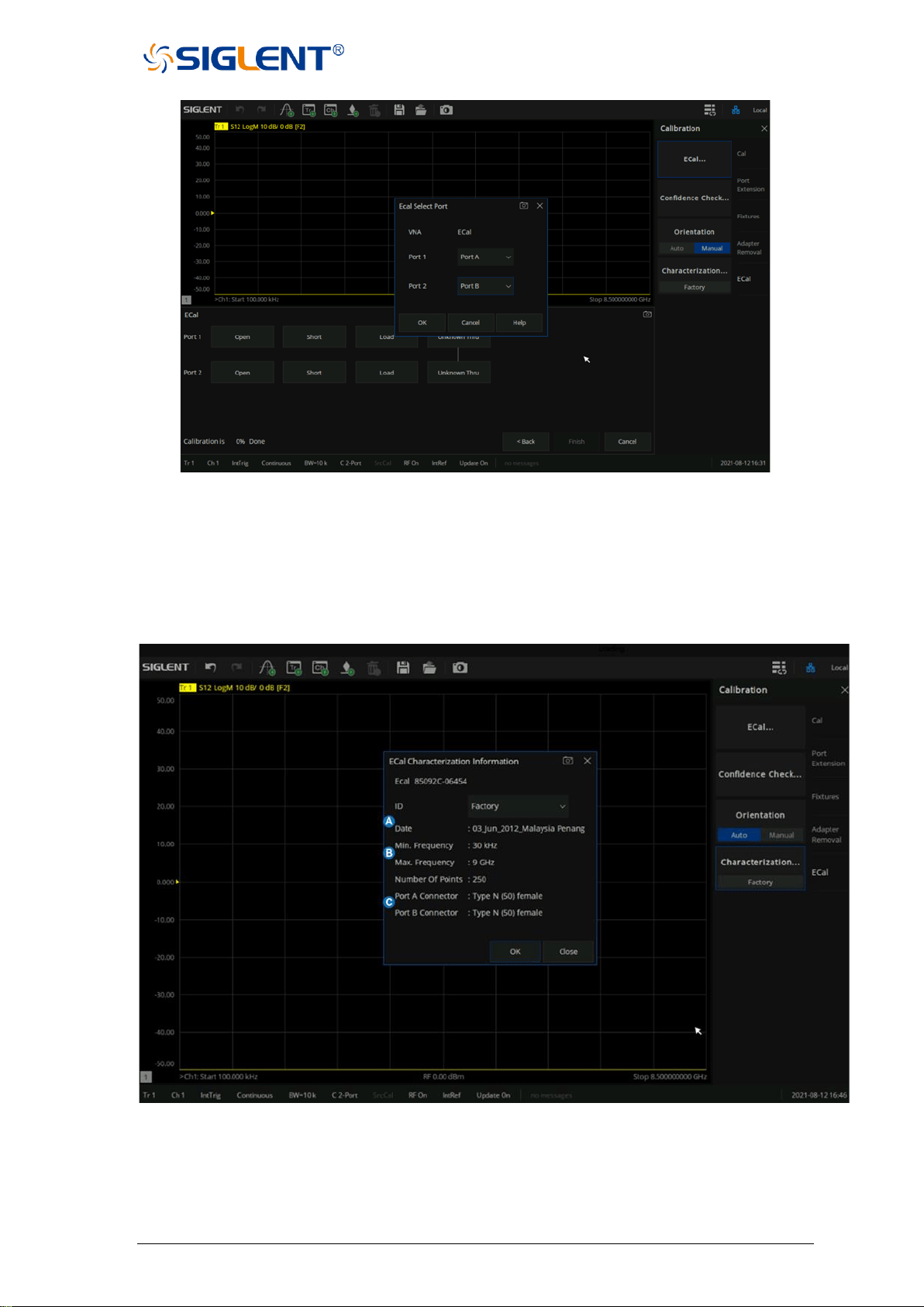
SNA5000A Vector Network Analyzer User Manual 92
Figure 3-41 Manual port setting
3.9.5 Characterization
Press “Cal” on the front panel, press “Cal” >Cal >Characterization >Factory to view all the
parameters of the stored Characterization in the ECal module.
Figure 3-42 The factory information of Cal Kit
A. The date when the characteristics were measured
B. The stimulus conditions when the characteristics were measured
C. The information of the Connector type

93 SNA5000A Vector Network Analyzer User Manual
4 Data analysis
4.1 Marker
The marker can display defined measurement data of traces. Each trace can set nine
ordinary markers and one reference marker.
Ordinary marker:
Press the Marker button on the front panel, click Add Marker in the Marker submenu to
create a marker, then set the required test frequency. if there are many markers on the trace,
click Select to select the desired marker. After the marker is created, the measurement value
of the marker will be displayed at the top right of the window, and the value format is the same
as the format of the trace. We can click the Delete Marker command under the marker
submenu to delete the marker and select the marker to delete from the pop-up menu. When
a trace is deleted, all markers on the trace will be deleted. Click the All Off command under
the Marker submenu or the Marker Setup submenu to delete all markers on the current trace.
Reference marker:
Press the Marker button on the front panel, click Reference Marker in the Marker submenu,
make the On option selected then the Reference Marker will be created. By default, the
Reference Marker is created at the location of the current ordinary Marker. If there is no
ordinary Marker on the current trace, the Reference Marker will be created at the center of
the trace. Reference Markers are denoted by an R. After creating a Reference Marker, set
the Reference Marker as value discretization, fixed marker, and coupling, we can set the data
format of Reference Marker’s display value and view the Reference Marker’s value in the
marker table, but the Reference Marker cannot be set as a difference (delta) marker. Click
Reference Marker in the Marker submenu, select the Off option to delete the Reference
Marker.
Marker setting:
Press the Marker button on the front panel, set the current marker in the Marker Setup
submenu, we can make the following settings for the currently selected marker:
1. Difference (delta) display: The difference display mode is closed by default, to open the
difference display mode, click the Delta to select the On option,
then the marker’s value will display the difference between the
ordinary marker and the reference marker, and the marker’s
value is marked with "Δ". If a reference marker has not been
added to the trace, the reference marker will be automatically
set on the trace. To display the absolute value of the marker,
click the Delta again to select the Off option.
2. Value discretization: The value discretization mode is closed by default. Due to the
limited number of sampling points set on the trace, the data of
other points except the sampling points are based on the
interpolation value of the sampling point data, which is approximate

SNA5000A Vector Network Analyzer User Manual 94
to the actual data, not the real measured data. By setting the value
discretization of the marker, the value of the marker can only be
taken at the sampling point, which ensures that the marker’s value
is from the measurement data and not interpolated data. To open
the value discretization mode, click the Discrete to select the On
option, at this time, the data of the marker is only selected from the
sampling points, when the coordinate value of the marker is not in
the sampling point, the marker is automatically moved to the nearest
sampling point. To turn off the value discretization, click the Discrete
to select the Off option.
3. Fixed marker: The fixed marker mode is closed by default. Fixed markers have
a fixed excitation position (x-axis coordinate), its response value (Y-axis
coordinate) will change according to the trace data update. To keep the
fixed value of the marker unchanged, click the Type command to select
the Fixed option, then the marker’s value will keep the current value
unchanged, and the marker does not move up or down with the trace
update. To restore the marker real-time update, click the Type command
again to select the Normal option.
4. Data format: The newly created marker uses the current trace’s data format by default.
To change the data format of the marker, click the Format and select the
corresponding data format in the pop-up menu. The following data formats are
available:
⚫ Trace Default
⚫ Log/Phase
⚫ Lin/Phase
⚫ Re/Im
⚫ R+jx
⚫ G+jB
⚫ Log Magnitude
⚫ Lin Magnitude
⚫ Phase
⚫ SWR
⚫ Delay
⚫ Real
⚫ Imaginary
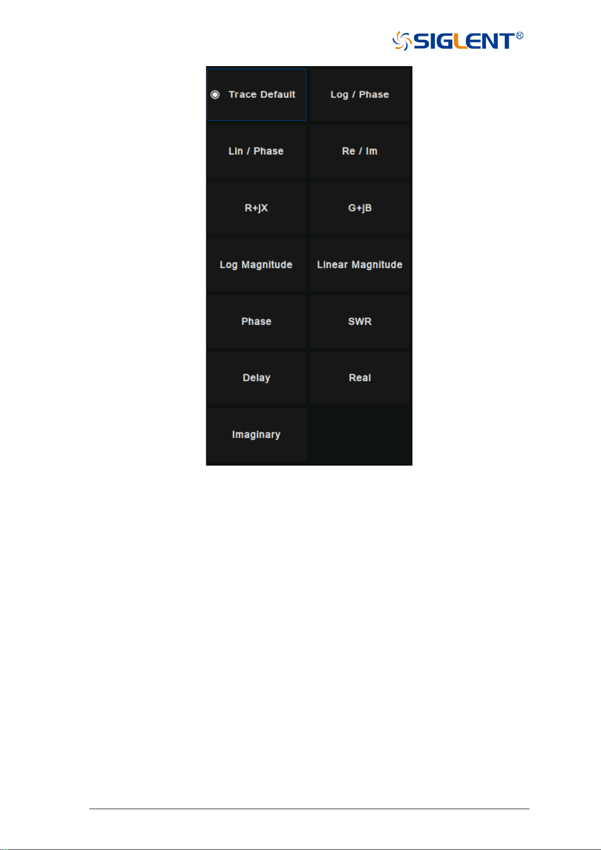
95 SNA5000A Vector Network Analyzer User Manual
Figure 4-1 Data format interface
5. Marker coupling: The newly created marker turns off coupling by default. At this time,
the marker is only set on a single trace, and the markers on different
traces do not affect each other. If we need multiple markers on different
traces to share settings, we can use the marker coupling function. Click
the Coupled command, and select the range of the marker coupling in
the pop-up menu for coupling operation. When the marker coupling
mode is on, the markers of the same number and X-axis (such as
frequency or time) on all traces in the coupling range share the settings,
and the marker’s setting on the current trace will be used by default. If
the current marker is not in the coupling range, the marker with the same
number on the trace with the smallest trace number is used.
Note: when the marker coupling mode is on, the marker on the trace
within the coupling range will automatically move to the same X-axis
coordinate.
6. Marker table: The newly created marker closes the marker table by default. If we need to
display all marker data in the form of a table, we can use the marker table

SNA5000A Vector Network Analyzer User Manual 96
function. Click the Marker Table to select the On state, a table will appear
at the bottom left to display all marker’s values, click the Marker Table again
to select the Off option to close the marker table.
Marker function:
Press the Marker button on the front panel, use the current marker to set the excitation in
the Marker Function submenu. Use the currently selected marker to achieve the following
functions:
⚫ Marker → Start:
Set the current marker position (X coordinate) as the sweeping starting point.
⚫ Marker → Stop:
Set the current marker position (X coordinate) as the sweeping ending point.
⚫ Marker → Center:
Set the current marker position (X coordinate) as the sweeping center point. Note:
When using this command, the sweeping boundary value far from the current marker
will be changed to reduce the sweeping range, so that the marker position becomes
the new sweeping center point.
⚫ Marker → Span:
This function is only available when the current marker is a difference (delta) marker.
Set the sweeping range between the current marker position and the reference
marker position (x coordinate).
⚫ Marker → Ref Level:
Set the response value (Y coordinate) of the current marker to the reference level of
the current trace.
⚫ Marker → Delay:
Referring to the phase slope of the current marker position, the line length is adjusted
to the receiver input, this function helps to smooth the phase trace around the current
marker. For the equipment without constant group delay in the measurement
frequency span, another electrical delay adjustment is needed. This function can be
used to measure electrical length or deviation from a linear phase. This function
requires the measured phase difference, so it is only suitable for proportional
measurements.
⚫ Marker → CW Freq:
Set the current marker position (frequency) to continuous wave (CW) frequency. This
function requires the x-axis field of the current marker, otherwise, it is invalid. After
changing CW frequency with this command, enable power or CW sweeping to apply
the changed CW frequency setting.
⚫ Marker → SA:
If the current mode is SA, the center frequency is set to the current marker value; If it
is not SA mode, then switch to SA mode, set the center frequency to the current
marker value, and set span to 10 times of the previous step freq.
Marker search function:

97 SNA5000A Vector Network Analyzer User Manual
The marker can be used to search the maximum value, minimum value, peak value, and
target value of the trace in the specified search domain. It can also search for multi-peak value,
multi-target, bandwidth filtering, and band-stop filtering.
1. Search domain:
The search domain is the frequency span included in a marker search operation. Each
marker has an independent search domain, and the default is full span, which is the same as
the current sweep range. The X coordinate movement range of the marker is limited in its
search domain. The user can set up up to 16 custom search domains. The search domains
are independent of each other and allowed to overlap. The search field can be set for each
marker, and multiple markers are allowed to share one search domain.
To set a custom search domain, press the Search button on the front panel, click the
Domain command in the Search submenu, and click the Add command in the pop-up menu.
Then click the Domain command again, click and select the newly created custom search
domain in the pop-up menu, and enter the required values in the Start and Stop text boxes
below the domain command. When the search domain of the current marker is not full span,
the indicator "Δ" will appear on the x-axis to identify the search domain of the current marker.
To delete a user-defined search domain, click the Domain command, select the search domain
to be deleted in the pop-up menu, then click the Domain command again, and then click Delete
in the pop-up menu. If the search domain of the marker is deleted, its search domain is
automatically set to full span.
2. Max and min search:
Press the Search button on the front panel and click the Max Search command in the
Search submenu to move the current marker to the maximum response value in the search
domain. Press the Search button on the front panel and click the Max Search command in
the Search submenu to move the current marker to the maximum response value in the search
domain. Click the Min Search command to move the current marker to the minimum response
value in the search domain.
3. Peak search:
Press the Search button on the front panel to search the peak in the Peak submenu.
Before searching for the peak value, the effective peak value to be searched should be defined
first. The validity of the peak value is determined by the search domain, peak polarity, threshold,
and deviation:
Peak polarity: According to the polarity, the peaks are divided into two categories:
Positive and negative. The positive peak value refers to situations where
the measured value is greater than the measured value at both ends of a
span, and the negative peak value refers to the peak value that the
measured value is less than the measured value at both ends of a span.
Click the Peak Polarity command in the Peak submenu to select the
peak polarity. The Both option means that both positive and negative
peaks are regarded as valid peaks for the search.

SNA5000A Vector Network Analyzer User Manual 98
Threshold: For the positive peak, only the peak whose measured value is greater
than the threshold is considered valid; for the negative peak, only the peak
whose measured value is less than the threshold is considered valid; when
the polarity of the peak is set to Both, the threshold is not used as the basis
for judging the validity of the peak. To set the threshold, click the Threshold
command in the Peak submenu to enter the required value.
Deviation: The deviation value of peak value refers to the smaller difference between the
measured value of peak value and the measured value of an adjacent peak
with the opposite polarity. Only the peak value with a deviation greater than
the rated value is considered valid. To set the deviation value, click the
Excursion command in the Peak submenu to enter the required value.
After determining the effective peak range and search domain, the peak
search can be started. There are several peak searching modes available:
⚫ Using the Peak Search command in the Peak submenu, the peak with the largest
measured value among the effective positive peaks or the peak with the smallest
measured value among the effective negative peaks will be included in the search
according to the peak polarity setting. If the current peak polarity is set to Both, the
peak with the largest measured value among the effective positive peaks is searched.
⚫ Use the Peak Right → Search command in the Peak submenu to search the nearest
effective peak from the current marker position to the right.
⚫ Use the Peak Left ← Search command in the Peak submenu to search the nearest
effective peak from the current marker position to the left.
⚫ Use the Next Peak Search command in the Peak submenu to search for the
effective positive peak value next lower than the current marker measurement value
or the effective negative peak value next higher than the current marker
measurement value according to the peak polarity setting. If the current peak polarity
is set to Both, the effective peak next lower than the current vernier measurement
value is searched.
4. Target search:
Press the Search button on the front panel to search the target in the Target submenu.
Before searching the target, set the target value and transition type:
Target value: The target value refers to the response value to search (Y coordinate). If
the response value of a point on the trace is equal to the target value, then
the point is the target point to search. To set the target value, click the
Target Value command in the Target submenu to enter the required value.
Transition type: The target points are divided into two types, positive and negative. The
positive target conversion type means that the measured value on the

99 SNA5000A Vector Network Analyzer User Manual
right side of the target point is greater than that on the left side, while
the negative target conversion type means that the measured value on
the right side of the target point is less than that on the left side. Click
the Transition command in the Target submenu to select the
conversion type to search for. The Both option means that both
positive and negative target conversion types are regarded as valid
targets.
After the target value, transition type and search domain are
determined, the target search can be started. The vector network
analyzer has the following target search modes:
⚫ Use the Target Search command in the Target submenu to search for the nearest
effective target from the current marker position to the right. When no effective target
can be found from the right, search from the starting point of the search domain to
the right.
⚫ Use the Target Right → Search command in the target submenu to search the
nearest valid target from the current marker position to the right.
⚫ Use the Target Left ← Search command in the Target submenu to search the
nearest valid target from the current marker position to the left.
5. Multi-peak search:
Press the Search button on the front panel to search for multiple peaks in the Multi
Peak & Target submenu. Before searching for multiple peaks, you need to set the threshold,
deviation, and peak polarity in the Peak Threshold, Peak Excursion and Peak Polarity
commands in the submenu to define the peak validity. After setting the above parameters,
click the Multi Peak Search command to search all effective peaks from the starting point of
the search domain to the right, and mark the peaks with a marker. Since there can only be 9
common markers on a single trace, only the first 9 effective peaks can be found when there
are many effective peaks.
6. Multi-target search:
Press the Search button on the front panel to search for multiple targets in the Multi
Peak & Target submenu. Before multi-target search, you need to set the target value and
conversion type in the Target Value and Transition submenu to define the target validity.
After setting the above parameters, click the Multi-Target Search command to search all
valid targets from the starting point of the search domain to the right, and mark the searched
targets with a marker. Since there can only be 9 common markers on a single trace, only the
first 9 valid targets can be found when there are many valid targets.
7. Tracking search:
When using the above search function, the marker position is only based on the current
sweeping result, and will not be dynamically updated with the trace update after the search.
Tracking mode can be used to update search results with trace data. Press the Search
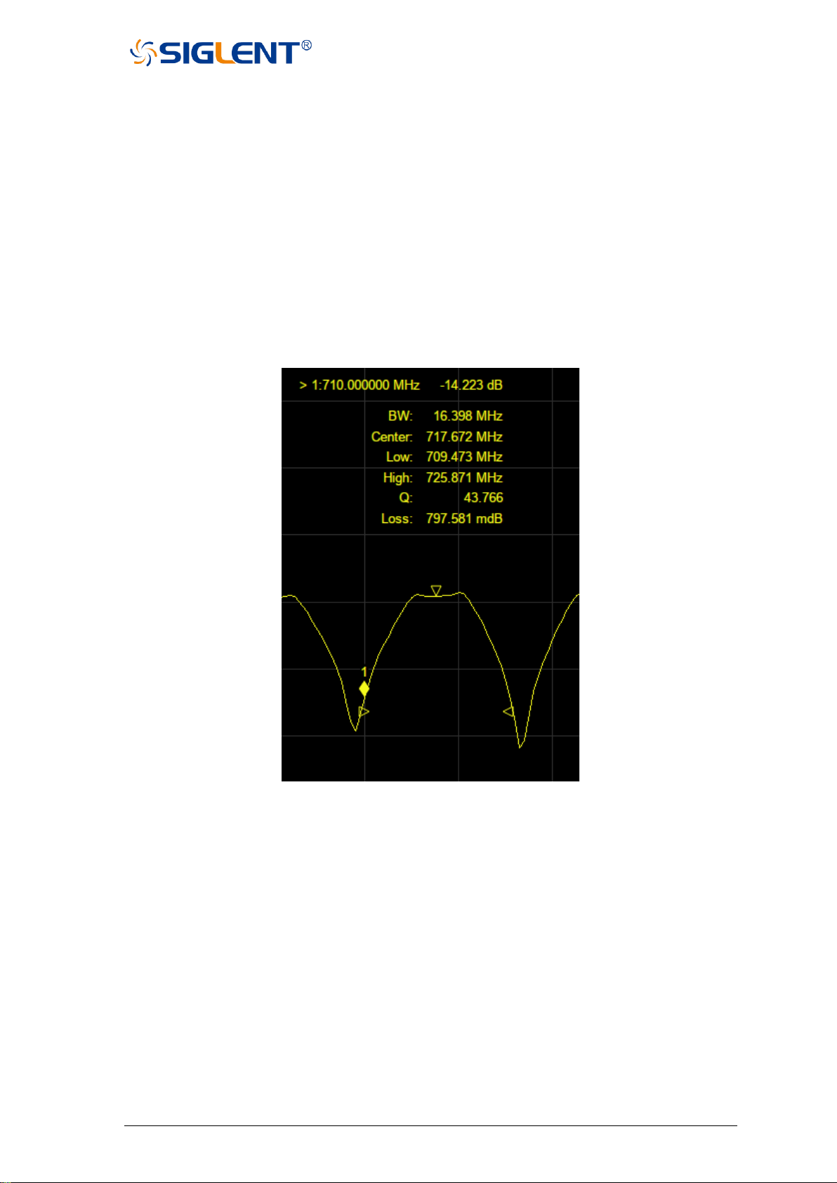
SNA5000A Vector Network Analyzer User Manual 100
button on the front panel, click the Tracking command, and select the search type in the
pop-up menu; the search in the tracking mode uses the search parameter settings in the
above search.
8. Bandwidth search:
Press the Search button on the front panel to search the bandwidth in the Bandwidth
submenu. Click BW Search Enable and select the On option to search the bandwidth. After
the bandwidth search is completed, a small triangle will be used to mark the cut-off frequency
of the trace, and the bandwidth, center frequency, cut-off frequency, quality factor, and
insertion loss will be displayed in the upper right corner of the window. To turn off the
bandwidth search, click BW Search Enable again and select the Off option. You can set
whether to alarm when the bandwidth search fails in the Sound On Fail command.
Figure 4-2 Bandwidth search example
9. Notch search:
Press the Search button on the front panel to search the band stop in the Notch submenu.
Click the Notch Search Enable command and select the On option to perform the band stop
search. After the band stop search is completed, a small triangle will be used to mark the cut-
off frequency of the trace, and the bandwidth, center frequency, cut-off frequency, quality factor,
and insertion loss will be displayed in the upper right corner of the window. To turn off the band
stop search, click the Notch Search Enable command again and select the Off option. You
can set whether to alarm when the band stop search fails in the Sound On Fail command.
4.2 Mathematical operation
The vector network analyzer supports saving the current data-trace in memory. It can

101 SNA5000A Vector Network Analyzer User Manual
perform four kinds of mathematical operations on the current data-trace and memory trace. In
addition, it can calculate and display statistical data (mean, standard deviation, and peak-peak)
on the data-trace. In addition, through the built-in formula editor, you can use multiple types of
traces from the same or different channels to build custom formulas. When the mathematical
operation with memory trace needs to be carried out, the current data needs to be stored in
memory first. Click Data→Memory to complete the storage operation. In the Display menu
bar, you can select three display modes: Display data-trace only, display memory trace and
display data-trace and memory trace at the same time. The four mathematical operations of
data-trace and memory trace are as follows, in which the values on data-trace and memory
trace are linear:
⚫ Data/Memory: Divide the measured data by the data in the stored trace. This
function can be used to calculate the ratio of two traces (such as
calculating gain or attenuation), which can also be regarded as the
normalization operation of test data.
⚫ Data*Memory: The current measurement data is multiplied by the data in
memory.
⚫ Data+Memory: Current measurement data plus data in memory.
⚫ Data–Memory: Current measurement data minus data in memory. For example,
you can use this function to store measured data, The error is then
subtracted from the DUT measurement.
4.3 Conversion
The vector network analyzer supports parameter conversion, which can convert the S
parameter of the current trace to the required parameter mode. The vector network analyzer
supports the following 8 conversion types.
⚫ Z-Reflect: Impedance in reflection measurement Z
r
.
⚫ Z-Transmit: Impedance in transmission measurement Z
t
.
⚫ Z-Trans-Shunt: Impedance in parallel transmission Z
t
.
⚫ Y-Reflect: Reflection measurement admittance Y
r
.
⚫ Y -Transmit: Admittance in transmission measurement Y
t
.
⚫ Y -Trans-Shunt: Admittance in parallel transmission Y
t
.
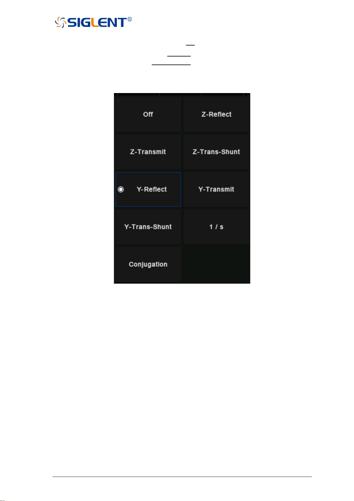
SNA5000A Vector Network Analyzer User Manual 102
⚫ 1/S: Reciprocal of S parameter.
⚫ Conjugation: Convert the measured value to a complex conjugate number.
Figure 4-3 Parameter conversion type
When both the fixture simulation measurement function and the port impedance function
are in the "on" state, the system will use the value set in the port impedance conversion. In
other cases, the system Z
0
(preset value: 50 Ω) will be used. The operation steps for selecting
the conversion type are as follows:
1. Click Math→Analysis→Conversion enter the selection interface.
2. Select the corresponding conversion type, effective immediately.
4.4 Equation editor
In the equation editor, we can input the algebraic formulas of standard mathematical
operators and functions, and reference the data available in the vector network analyzer. After
a valid formula is entered and enabled, the working trace will be displayed as the result of the
set formula and updated in real-time.
For example, enter the formula S21/(1 - S11). The trace is calculated by dividing each S21
data point by 1 and subtracting the value of the corresponding S11 data point. For a 201 point
sweep, the calculation is repeated 201 times, once per point. In addition, suppose that the
vector network analyzer is required to measure the directivity of a 3-port device to be tested,
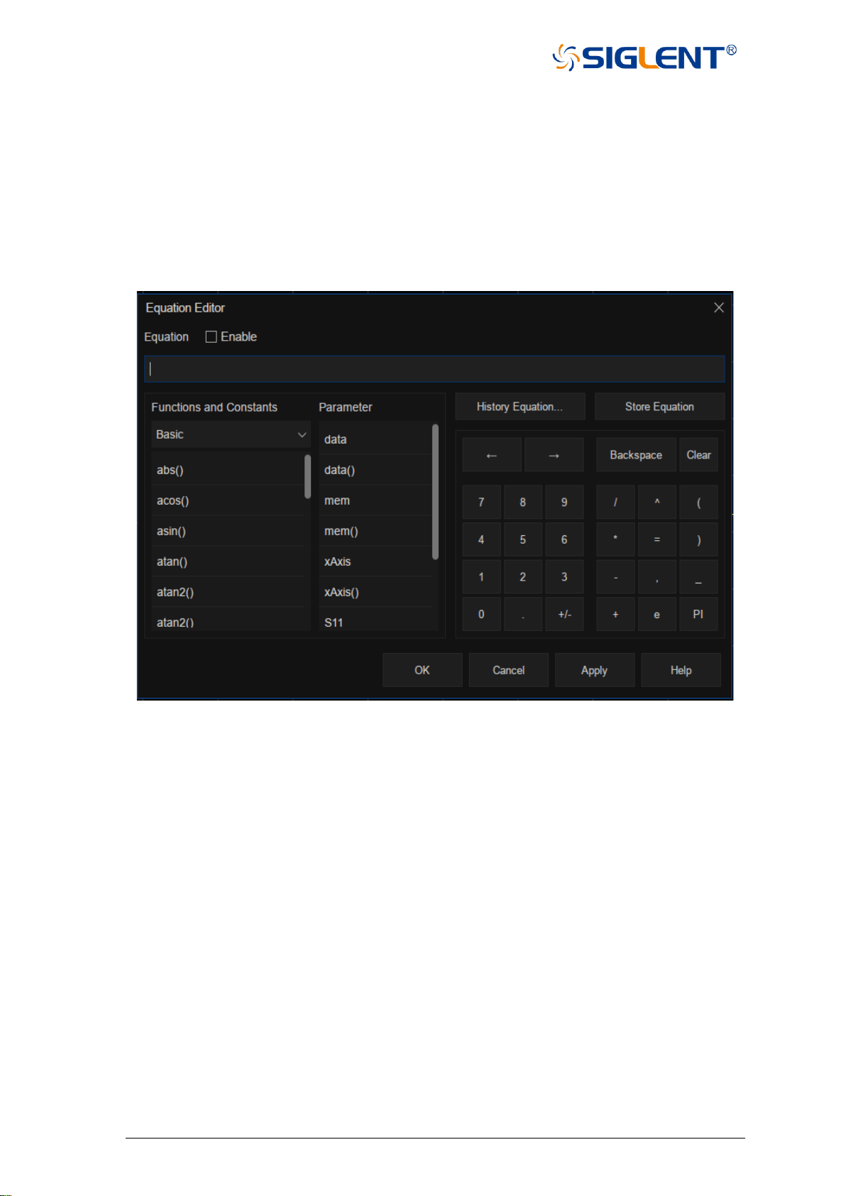
103 SNA5000A Vector Network Analyzer User Manual
and the directivity is not the measurement parameter of the vector network analyzer, then the
formula editor can be used to complete the measurement, and the result is the sum and
difference of the traces in logarithmic amplitude format, that is S12 + S23 - S13. Because the
formula editor operates on linear complex data, the actual required formula is S12 * S23 / S13.
Finally, the vertical axis format is set to logarithmic amplitude for display. The operation
steps of the equation editor are as follows:
1. Click Math→Analysis→Equation Editor enter the equation editor interface.
Figure 4-4 Formula editor interface
2. In the formula edit box, enter functions, operators, and data to form the formula.
3. After setting the formula, click OK to exit the formula editing interface and click
the Equation status to On to take effect.
Introduction to formula editor interface:
⚫ Enable: Select the box to enable the currently entered formula, and clear the box to
disable the currently edited formula. If the data traces used are from other
channels instead of formula traces, these channels must have the same
number of data points to be valid channels.
⚫ Functions and Constants: It stores some commonly used functions and constants,
as well as other functions set by the system.
⚫ Parameter: Select the items that need to be measured only from the working
channel.
⚫ History Equation: Used to save previously-stored formulas.
⚫ Store Equation: Store the current input formula to facilitate subsequent use.

SNA5000A Vector Network Analyzer User Manual 104
⚫ : Move the cursor to the left without clearing the characters.
⚫ →: Move the cursor to the right without clearing the character.
⚫ Backspace: Clear the character while moving the marker to the left.
⚫ Clear: Clear the currently entered formula.
⚫ Numbers, operators, and constants: Numbers, common operators, and constants.
Description of functions and constants in formula editor:
Common functions
Description
Abs (complex a)
Returns the sqrt(a.re*a.re+a.im*a.im)
Acos (scalar a)
Returns the arc cosine of a in radians
Asin (scalar a)
Returns the arc sine of a in radians
Atan (scalar a)
Returns the arc tangent of a in radians
atan2 (complex a)
Returns the phase of a = (re, im) in radians
atan2 (scalar a, scalar b)
Returns the phase of (a, b) in radians
Conj (complex a)
Returns the conjugate of a
Cos (complex a)
Takes a in radians and returns the cosine
Cpx (scalar a, scalar b)
Returns a complex value (a+ib) from two
scalar values
Exp (complex a)
Returns the exponential of a
Im (complex a)
Returns the imaginary part of a as the scalar
part of the result (zeroes the imaginary part)
Ln (complex a)
Returns the natural logarithm of a
log10 (complex a)
Returns the base 10 logarithm of a
Mag (complex a)
Returns sqrt(a.re*a.re+a.im*a.im)
Phase (complex a)
Returns atan2(a) in degrees
Pow (complex a,complex b)
Returns a to the power b
Re (complex a)
Returns the scalar part of a (zeroes the
imaginary part)
Sin (complex a)
Takes a in radians and returns the sine
Sqrt (complex a)
Returns the square root of a, with phase
angle in the half-open interval (-pi/2, pi/2]
Tan (complex a)
Takes a in radians and returns the tangent
Constant
e
2.71828182845904523536
PI
3.14159265358979323846
Advanced function
Description
A (complex a, complex b, complex c, complex d)
F11 conversion = ((1+a)*(1-d) + b*c)/(2*b)
A (scalar i, scalar j)
returns A(Sii, Sji, Sij, Sjj)
B (complex a, complex b, complex c, complex d)
F12 conversion = Z0*((1+a)*(1+d) - b*c)/(2*b)
B (scalar i, scalar j)
returns B(Sii, Sji, Sij, Sjj)

105 SNA5000A Vector Network Analyzer User Manual
C (complex a, complex b, complex c, complex d)
F21 conversion = (1/Z0)*((1-a)*(1-d) - b*c)/(2*b)
C (scalar i, scalar j)
returns C(Sii, Sji, Sij, Sjj)
D (complex a, complex b, complex c, complex d)
F22 conversion = ((1-a)*(1+d) + b*c)/(2*b)
D (scalar i, scalar j)
returns D(Sii, Sji, Sij, Sjj)
H11 (complex a, complex b, complex c, complex d)
H11 conversion = Z0*((1+a)*(1+d) - b*c)/((1-a)*(1+d)
+ b*c)
H11 (scalar i, scalar j)
returns H11(Sii, Sji, Sij, Sjj)
H12 (complex a, complex b, complex c, complex d)
H12 conversion = 2*c/((1-a)*(1+d) + b*c)
H12 (scalar i, scalar j)
returns H12(Sii, Sji, Sij, Sjj)
H21 (complex a, complex b, complex c, complex d)
H21 conversion = -2*b/((1-a)*(1+d) + b*c)
H21 (scalar i, scalar j)
returns H21(Sii, Sji, Sij, Sjj)
H22 (complex a, complex b, complex c, complex d)
H22 conversion = (1/Z0)*((1-a)*(1-d) - b*c)/((1-
a)*(1+d) + b*c)
H22 (scalar i, scalar j)
returns H22(Sii, Sji, Sij, Sjj)
Kfac (complex a, complex b, complex c, complex d)
k-factor = (1 - abs(a)^2 - abs(d)^2 + (abs(a*d -
b*c)^2)/(2*abs(b*c))
Kfac (scalar i, scalar j)
returns kfac(Sii, Sji, Sij, Sjj)
MAPG (complex a, complex b, complex c, complex
d)
maximum available power gain =
abs(b/c)*(kfac(a,b,c,d) - sqrt(kfac(a,b,c,d)^2 - 1))
MAPG (scalar i, scalar j)
Returns MAPG(Sii, Sji, Sij, Sjj)
MSG (complex a, complex b, complex c, complex d)
maximum stable power gain = abs(b)/abs(c)
MSG (scalar i, scalar j)
Returns MSG(Sii, Sji, Sij, Sjj)
mu1 (complex a, complex b, complex c, complex d)
μ-factor = (1 - abs(a)^2) / (abs(d - conj(a) * (a*d-b*c))
+ abs(b*c))
mu1 (scalar i, scalar j)
Returns mu1(Sii, Sji, Sij, Sjj)

SNA5000A Vector Network Analyzer User Manual 106
mu2 (complex a, complex b, complex c, complex d)
μ-factor = (1 - abs(d)^2) / (abs(a - conj(d) * (a*d-b*c))
+ abs(b*c))
mu2 (scalar i, scalar j)
Returns mu2(Sii, Sji, Sij, Sjj)
T11 (complex a, complex b, complex c, complex d)
T11 conversion = -(a*d - b*c)/b
T11 (scalar i, scalar j)
Returns T11(Sii, Sji, Sij, Sjj)
T12 (complex a, complex b, complex c, complex d)
T12 conversion = a/b
T12 (scalar i, scalar j)
Returns T12(Sii, Sji, Sij, Sjj)
T21 (complex a, complex b, complex c, complex d)
T21 conversion = -d/b
T21 (scalar i, scalar j)
Returns T21(Sii, Sji, Sij, Sjj)
T22 (complex a, complex b, complex c, complex d)
T22 conversion = 1/b
T22 (scalar i, scalar j)
Returns T22(Sii, Sji, Sij, Sjj)
Y11 (complex a, complex b, complex c, complex d)
Y11 conversion = (1/Z0)*((1-a)*(1+d) +
b*c)/((1+a)*(1+d) - b*c)
Y11 (scalar i, scalar j)
Returns Y11(Sii, Sji, Sij, Sjj)
Y12 (complex a, complex b, complex c, complex d)
Y12 conversion = (1/Z0)*(-2*c)/((1+a)*(1+d) - b*c)
Y12 (scalar i, scalar j)
Returns Y12(Sii, Sji, Sij, Sjj)
Y21 (complex a, complex b, complex c, complex d)
Y21 conversion = (1/Z0)*(-2*b)/((1+a)*(1+d) - b*c)
Y21 (scalar i, scalar j)
Returns Y21(Sii, Sji, Sij, Sjj)
Y22 (complex a, complex b, complex c, complex d)
Y22 conversion = (1/Z0)*((1+a)*(1-d) +
b*c)/((1+a)*(1+d) - b*c)
Y22 (scalar i, scalar j)
Returns Y22(Sii, Sji, Sij, Sjj)
Z11 (complex a, complex b, complex c, complex d)
Z11 conversion = Z0*((1+a)*(1-d) + b*c)/((1-a)*(1-d)
- b*c)
Z11 (scalar i, scalar j)
Returns Z11(Sii, Sji, Sij, Sjj)
Z12 (complex a, complex b, complex c, complex d)
Z12 conversion = Z0*(2*c)/((1-a)*(1-d) - b*c)
Z12 (scalar i, scalar j)
Returns Z12(Sii, Sji, Sij, Sjj)

107 SNA5000A Vector Network Analyzer User Manual
Z21 (complex a, complex b, complex c, complex d)
Z21 conversion = Z0*(2*b)/((1-a)*(1-d) - b*c)
Z21 (scalar i, scalar j)
Returns Z21(Sii, Sji, Sij, Sjj)
Z22 (complex a, complex b, complex c, complex d)
Z22 conversion = Z0*((1-a)*(1+d) + b*c)/((1-a)*(1-d)
- b*c)
Z22 (scalar i, scalar j)
Returns Z22(Sii, Sji, Sij, Sjj)
Channel parameter data
data
Corrected data
data(scalar i)
Corrected data of trace i (trace number)
mem
Memory data
mem(scalar i)
Memory data of trace i (trace number)
xAxis
X-axis data
xAxis(scalar i)
X-axis data of trace i (trace number)
S11 - S44
S-parameter data
Common H parameter, Y parameter, Z parameter, F parameter, and T parameter
definition(2-port network):
1) Mixing Parameter(H)
2) Admittance parameter(Y)
3) Impedance parameter(Z)
4) Basic parameter(F)
5) Scattering transmission parameter(T)
S parameter convert to H parameter, Y parameter, Z parameter, F parameter and T
parameter (2-port network):

SNA5000A Vector Network Analyzer User Manual 108
1) S parameter convert to H parameter
2) S parameter convert to Y parameter
3) S parameter convert to Z parameter
4) S parameter convert to basic parameter

109 SNA5000A Vector Network Analyzer User Manual
5) S parameter convert to T parameter
Description of formula editor’s operator:
Operator
Description
+
plus
-
minus
*
multiply
/
divide
^
power
(
opening parenthesis
]
closing parenthesis
,
comma, parameter separator
=
equal
E
exponent
Note: operator priority:
1. ^
2. *, /
3. +, -
4.5 Trace statistics
Click Math→Analysis→Statistics, set the status to On to open the statistics function. The
upper right corner of the interface will display the mean value, standard deviation, and peak to
peak value of the current working trace.
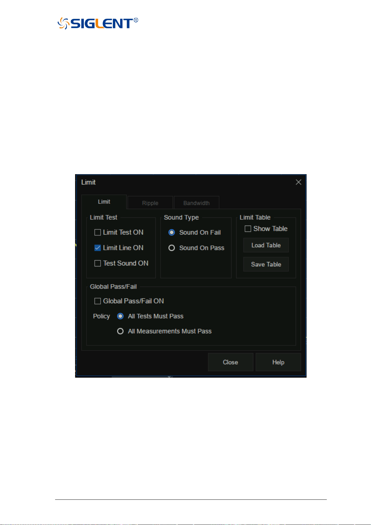
SNA5000A Vector Network Analyzer User Manual 110
Figure 4-5 Statistical data interface
4.6 Limit test
Limit Line is a test form that can visualize test data and results. The limit test compares
the measured data with the defined limit and provides the qualified or unqualified judgment
information of each measured data point. Limit line and limit test are not suitable for smith
chart and polar coordinate display formats, and limit line and limit test functions are
automatically disabled for these display types.
Limit table setting
Click Math→Analysis→Limit and the pop-up dialog box is shown in the figure below.
Limit test, sound type, limit table, global pass/fail can be set in this interface.
Figure 4-6 Limit test interface
Limit test:
⚫ Limit test on: Check this box to compare the data with the limit and display "pass"
or "Fail" judgment result.
⚫ Limit line on: Check this box to display the limit on the screen.
⚫ Sound on fail: When this box is selected, when the point on the trace fails in the limit
test, a beep will sound.
Sound type:
⚫ Sound on fail: When this box is checked, the equipment will beep when the test fails.
⚫ Sound on pass: When this box is checked, the equipment will beep when the test
passes.
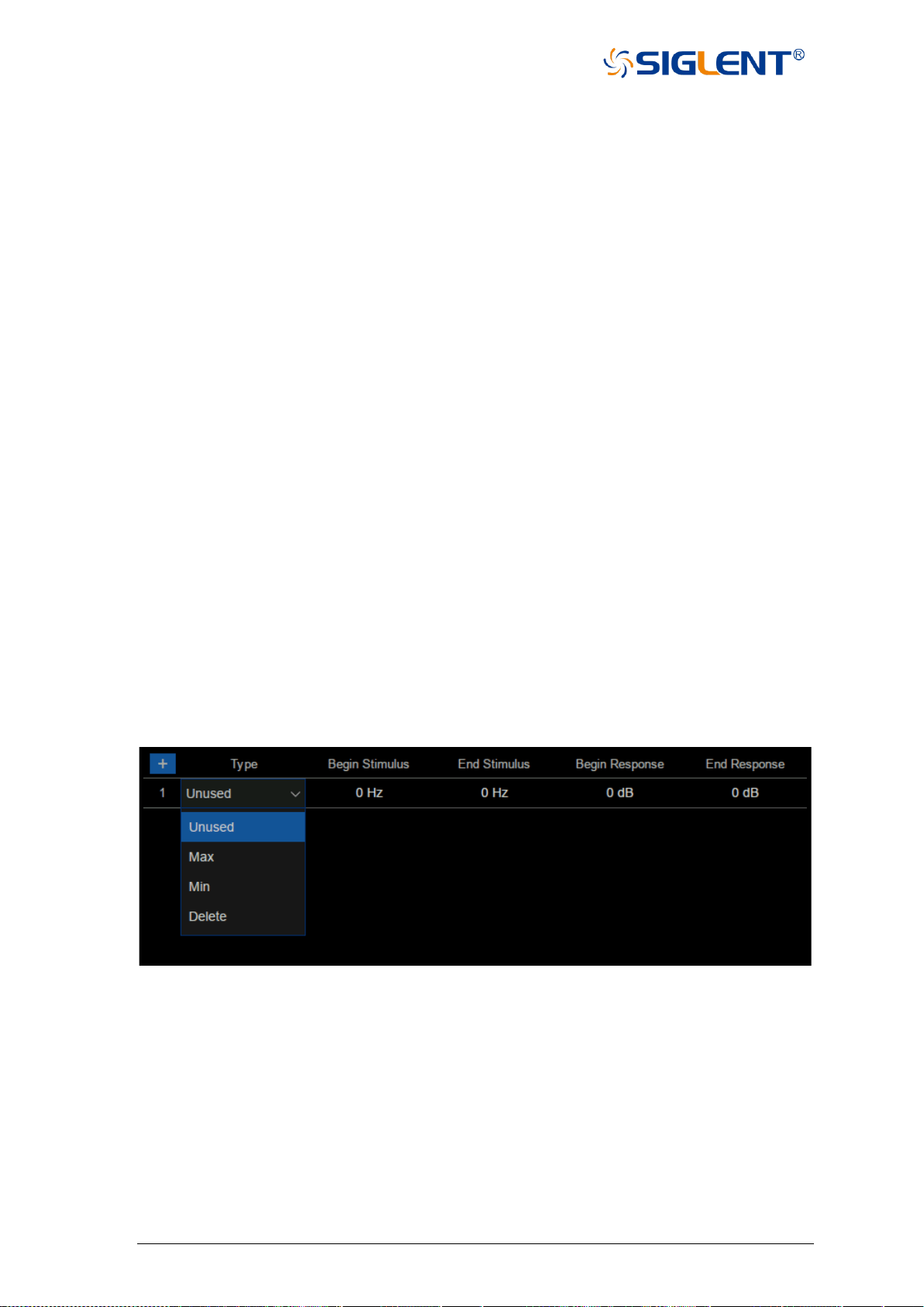
111 SNA5000A Vector Network Analyzer User Manual
Limit table:
⚫ Show table: Check this box to open a table at the bottom of the screen to create and
edit limits.
⚫ Load table: Call the saved limit table, The saved format of the limit table is CSV by default.
Global pass/fail:
Pass/fail indicator is a convenient way to monitor all measurement status.
Global pass/fail on - Check this box to display the global pass / fail status.
Policy - Select which of the following requirements must be met for the global pass/fail
status to display "pass":
⚫ All tests must pass - This setting will read the results from the limit test. If all tests
(limit test is on) pass, the global pass/fail status will be "pass".
⚫ All measurements must pass - Unless all measured data points are within the
established test limits and the limit test is "on", the
global pass/fail status will be "fail".
Note: In this mode, if there is a test that does not set the limit test to the on state, the global
pass/fail will display "fail".
Limit line setting
Click Math→Analysis→Limit Table→Limit to open the limit line setting interface, we
can also click Math→Analysis→Limit→Show Table to open the limit line setting interface,
as shown in the figure below.
Figure 4-7 Limit line setting interface
Limit line type:
⚫ Unused: Invalid limit line.
⚫ Max: Above this limit line, the measurement fails.
⚫ Min: Below this limit line, the measurement fails.
⚫ Delete: Delete limit line.
Begin stimulus: Frequency of the limit line’s starting point.
End stimulus: Frequency of the limit line’s ending point.
Begin response: Response of the limit line’s starting point.
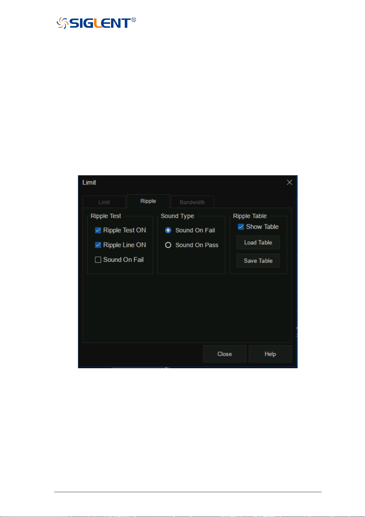
SNA5000A Vector Network Analyzer User Manual 112
End response: Response of the limit line’s ending point.
4.7 Ripple limit test
The ripple limit test function can be performed independently of the limit test function,
and the ripple limit can be set to evaluate whether the measurement result is qualified or
unqualified. Ripple is defined as the difference between the maximum value and the
minimum value within the specified excitation range. The ripple limit function is only
applicable to the measured point value, not to the interpolation.
Ripple table setting
Click Math→Analysis→Limit→Ripple to open the ripple test setting interface, we can
set ripple test, sound type, and ripple table in this interface.
Figure 4-8 Ripple test setting interface
Ripple test:
⚫ Ripple test on: Check this box to set the ripple test to "on" state and display "pass"
or "Fail".
⚫ Ripple line on: Check this box to display the ripple limit line on the screen.
⚫ Sound on fail: When this box is checked, the VNA will beep when the test fails.
Sound type:
⚫ Sound on fail: When this box is checked, the equipment will beep when the test fails.
⚫ Sound on pass: When this box is checked, the equipment will beep when the test
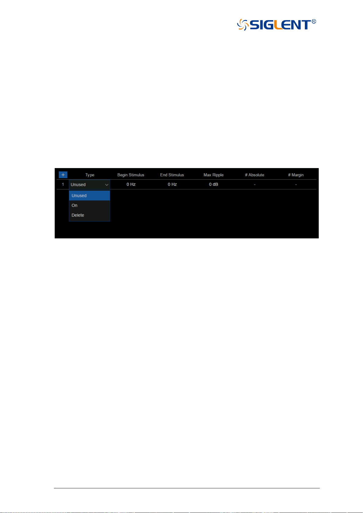
113 SNA5000A Vector Network Analyzer User Manual
passes.
Ripple table:
⚫ Show table: Check this box to display a table at the bottom of the screen for creating
and editing limits.
⚫ Load table: Call the saved ripple limit table.
⚫ Save table: Save the ripple limit table, the saved format of the ripple table is CSV by
default.
Ripple limit line setting
Click Math→Analysis→Limit Table→Ripple to open the ripple limit setting interface, we
can also click Math→Analysis→Limit→Ripple→Show Table to open the ripple limit setting
interface, as shown in the figure below.
Figure 4-9 Ripple limit setting interface
Type:
⚫ Unused: Invalid ripple test line.
⚫ On: Open ripple test limit line.
⚫ Delete: Delete ripple test limit line.
Begin stimulus: Frequency of ripple limit line’s starting point.
End stimulus: Frequency of ripple limit line’s ending point.
Max ripple: Maximum value of ripple test.
Absolute: The difference between the maximum and minimum in the frequency band.
Margin: The difference between the absolute value of ripple and the limit value.
4.8 Bandwidth limit test
The bandwidth limit test function can be used to test the bandwidth of a bandpass filter.
The bandwidth limit test can find the peak value in the bandwidth, and find the frequency points
lower than the specified value of the peak value on the left and right sides of the peak point,
and the frequency between these two points is the filter bandwidth, and then compare the
obtained bandwidth with the minimum and maximum allowable bandwidth specified in advance.
Bandwidth test setting
Click Math→Analysis→Limit→Bandwidth to open the broadband test setting interface,
we can set bandwidth test, sound type, and target bandwidth in this interface.
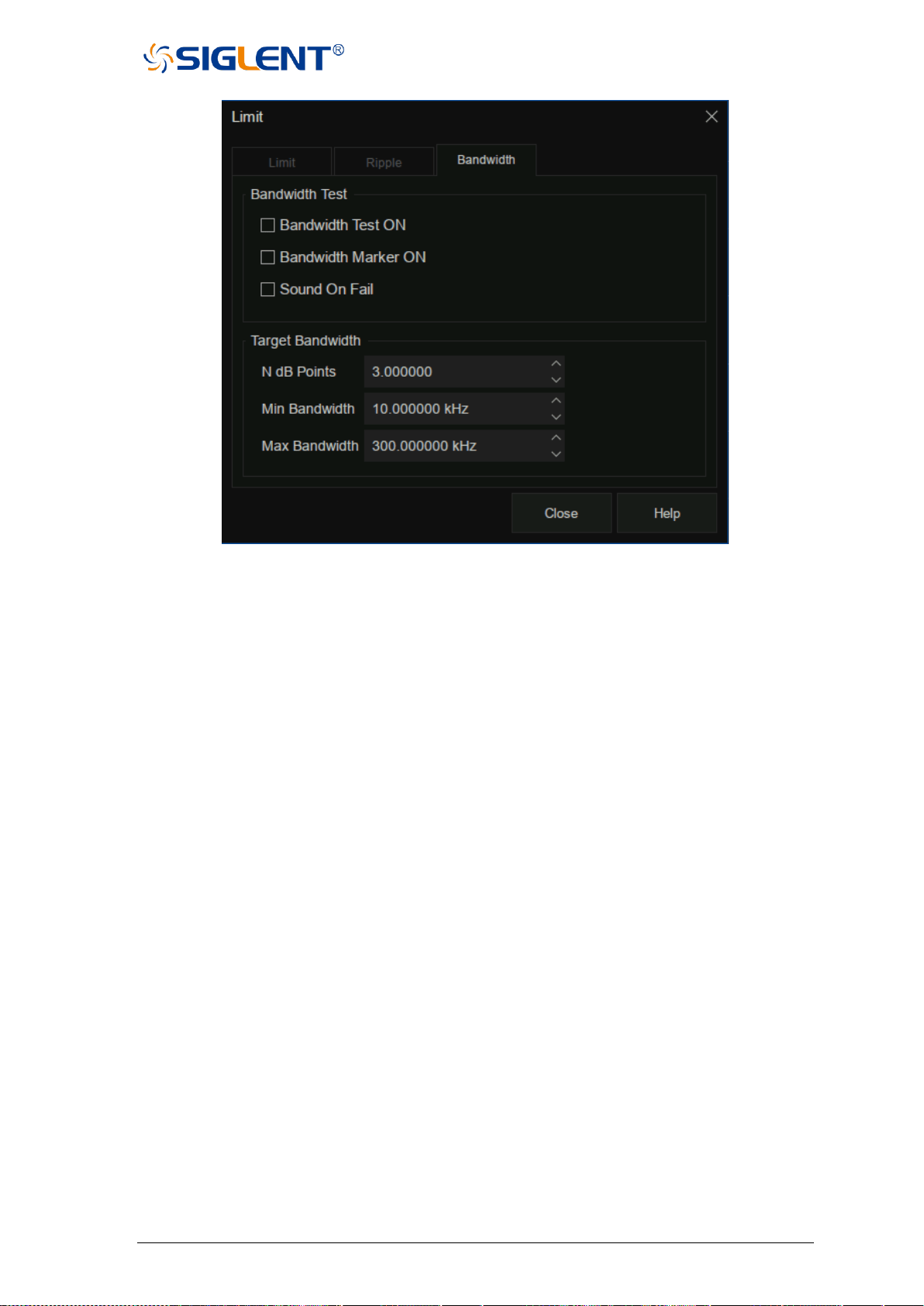
SNA5000A Vector Network Analyzer User Manual 114
Figure 4-10 Bandwidth test setting interface
Bandwidth test:
⚫ Bandwidth test on: Check this box to set the bandwidth limit test state to on.
⚫ Bandwidth marker on: Check this box to display the bandwidth on the screen.
⚫ Sound on fail: When this box is selected, an alarm will sound when the bandwidth
limit test fails.
Target bandwidth:
⚫ N dB points: Specifies the bandwidth threshold in dB.
⚫ Min bandwidth: Enter the lower limit of bandwidth in Hz.
⚫ Max bandwidth: Enter the upper limit of bandwidth in Hz.
Note: If the data format is Smith chart or polar coordinate format, the bandwidth test is skipped.
4.9 Time domain
A vector network analyzer is usually used to measure the frequency domain
characteristics of the DUT. For the time domain characteristics of the DUT, the frequency
domain parameters can be obtained by inverse Fourier transform. The time-domain
characteristics use time as the horizontal axis to display the measurement results. Then the
characteristics of the DUT can be observed from two different visual angles of frequency
domain and time domain by the vector network analyzer.
4.9.1 Transform
Click Math→Time Domain→Time Domain Setup→Transform to open the time domain
transform setting interface, we can set the start time, stop time, center time, span, transform
mode in this interface.
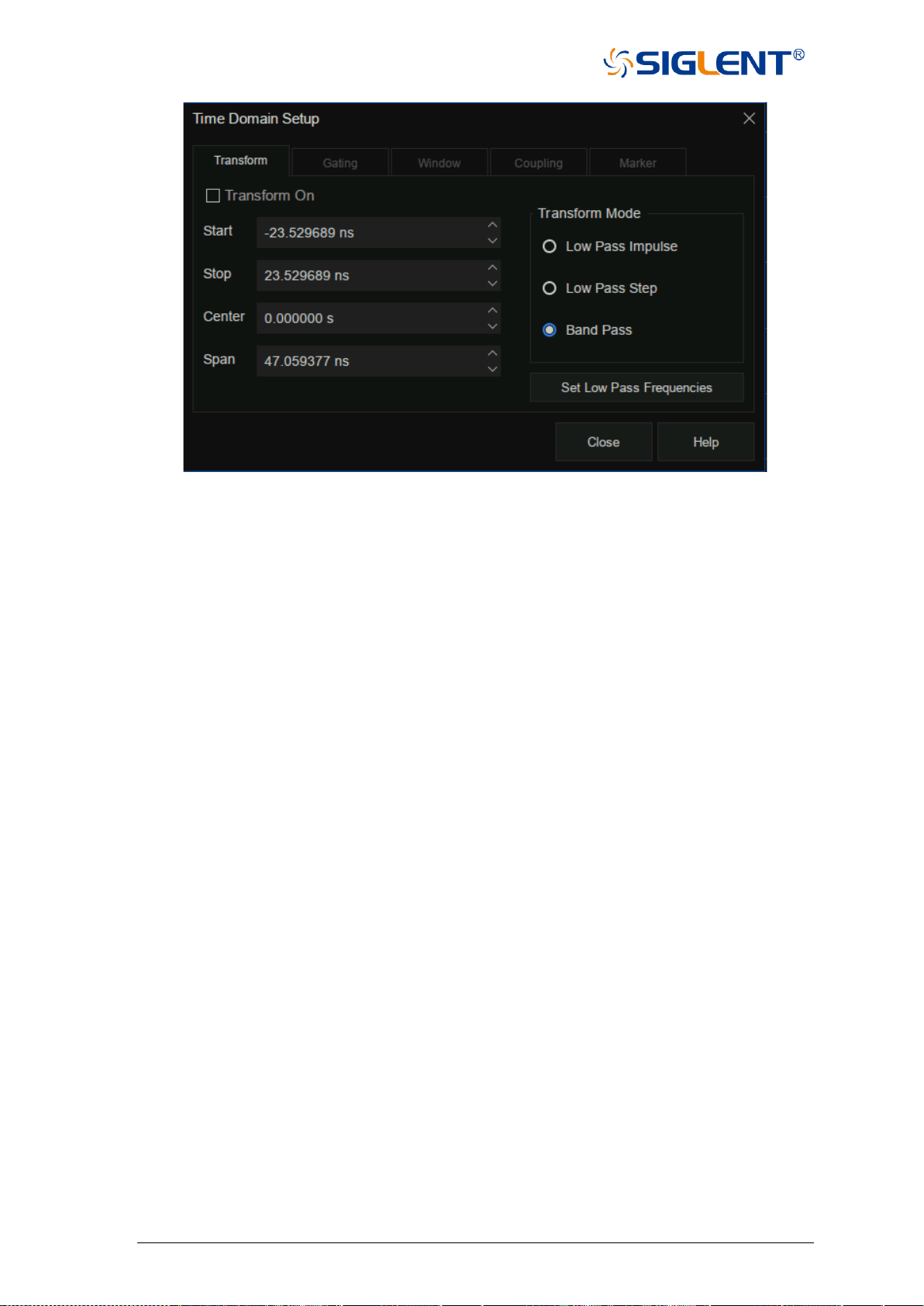
115 SNA5000A Vector Network Analyzer User Manual
Figure 4-11 Time domain setting interface
Transform switch: Check the transform switch to switch to time-domain mode.
Start time: Set the start time of transformation displayed.
Stop time: Set the stop time of transformation displayed.
Center time: Set the center time of transformation displayed.
Time span: Set the time span of the transformation displayed on the screen of VNA.
Transform mode:
⚫ Low pass impulse: High resolution, suitable for viewing the small response of the
device propagating low-frequency signal. In this low pass impulse
mode, the frequency expands to DC and negative frequency.
Therefore, when we click Set Low Pass Frequencies, the starting
frequency will be automatically adjusted, which will affect the
calibration accuracy. Therefore, it is necessary to calibrate after
setting the time domain measurement parameters.
⚫ Low pass step: The simplest way to determine the discontinuities caused by
inductors and capacitors in equipment that propagate low
frequency signals.
⚫ Bandpass: The simplest method, which can be used with any frequency sweep,
it is most useful when measuring devices with limited bandwidth.
Capacitance and inductance reactance will not be shown. For the same
frequency range and number of points, the bandwidth of bandpass mode is
twice that of impulse mode, which will hide the closely spaced response and
reduce the response resolution. The measurement range is inversely
proportional to the frequency step.
Set low pass frequencies: It can only be used in low pass mode. After clicking Set Low
Pass Frequencies, the measurement range is inversely
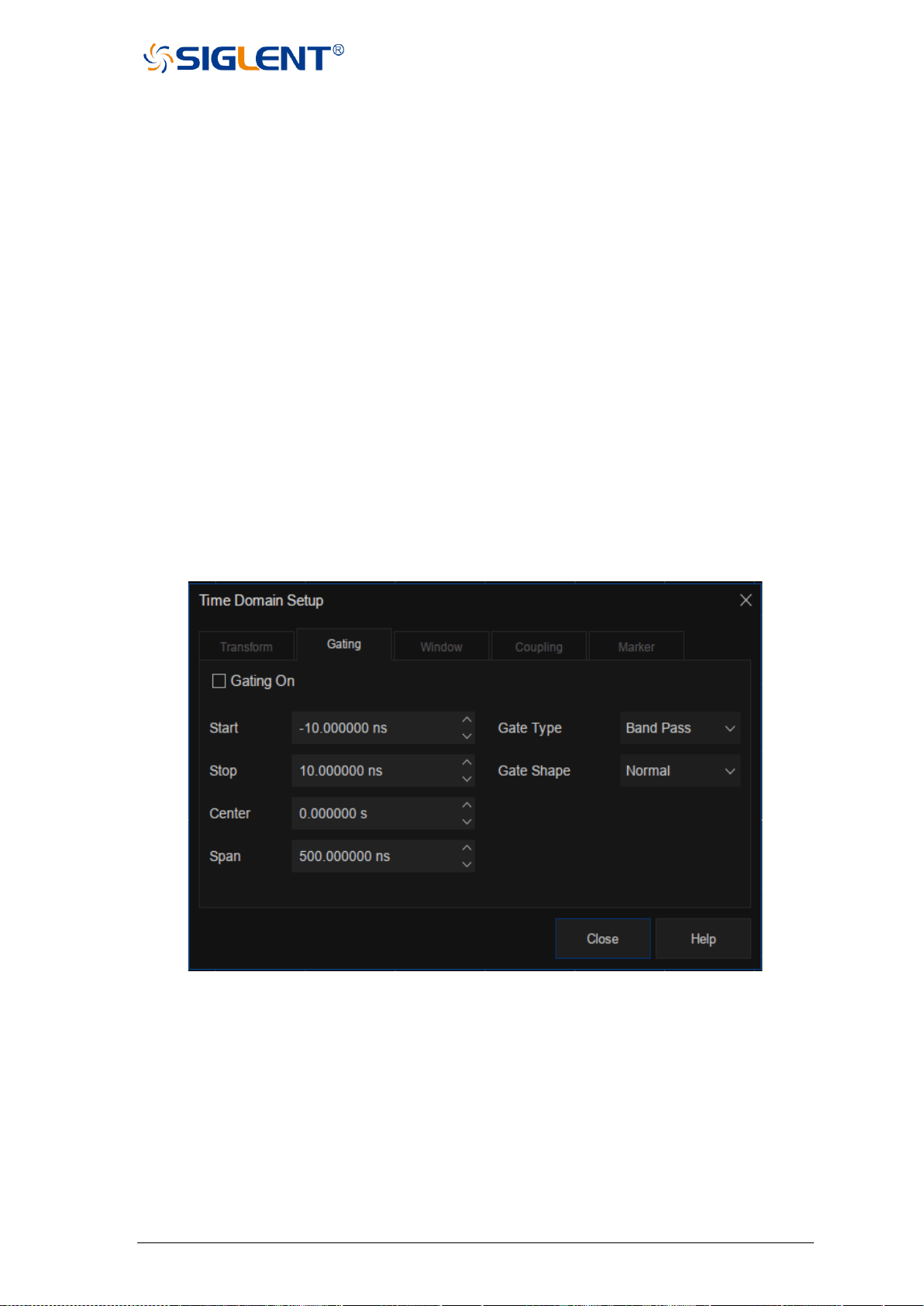
SNA5000A Vector Network Analyzer User Manual 116
proportional to the starting frequency. Recalculate the start
frequency and step frequency as the harmonics of the starting
frequency. Calculate the starting frequency according to the
formula of low pass start frequency = stop frequency/points. The
calculated value must not be less than the minimum frequency of
the vector network analyzer. The number of points or stop
frequency may change.
4.9.2 Gating
The gating function of a vector network analyzer is the most useful feature in time domain
transform. When the time domain characteristics of the equipment need to be viewed, the
gating function can only choose the required time-domain response, eliminate unnecessary
time domain response, and then view the frequency domain characteristic curve of the required
response through Fourier transform. The gating function enables the DUT to be characterized
without connectors or adapters.
Click Math→Time Gating→Gating Setup→Gating to open the gating setting interface,
then we could set the start time, stop time, center time, span, gate type, and gate shape in this
interface.
Figure 4-12 Gating setting interface
Gating on: Open or close the gating function.
Start time: Set the start time of gating.
Stop time: Set the stop time of the gate.
Center time: Set the center time of the gatie.
Time span: Set the time span of the gate.
Gate type: Sets the type of filtering performed by the gating function.
⚫ Bandpass: Keep the response in the gating span.
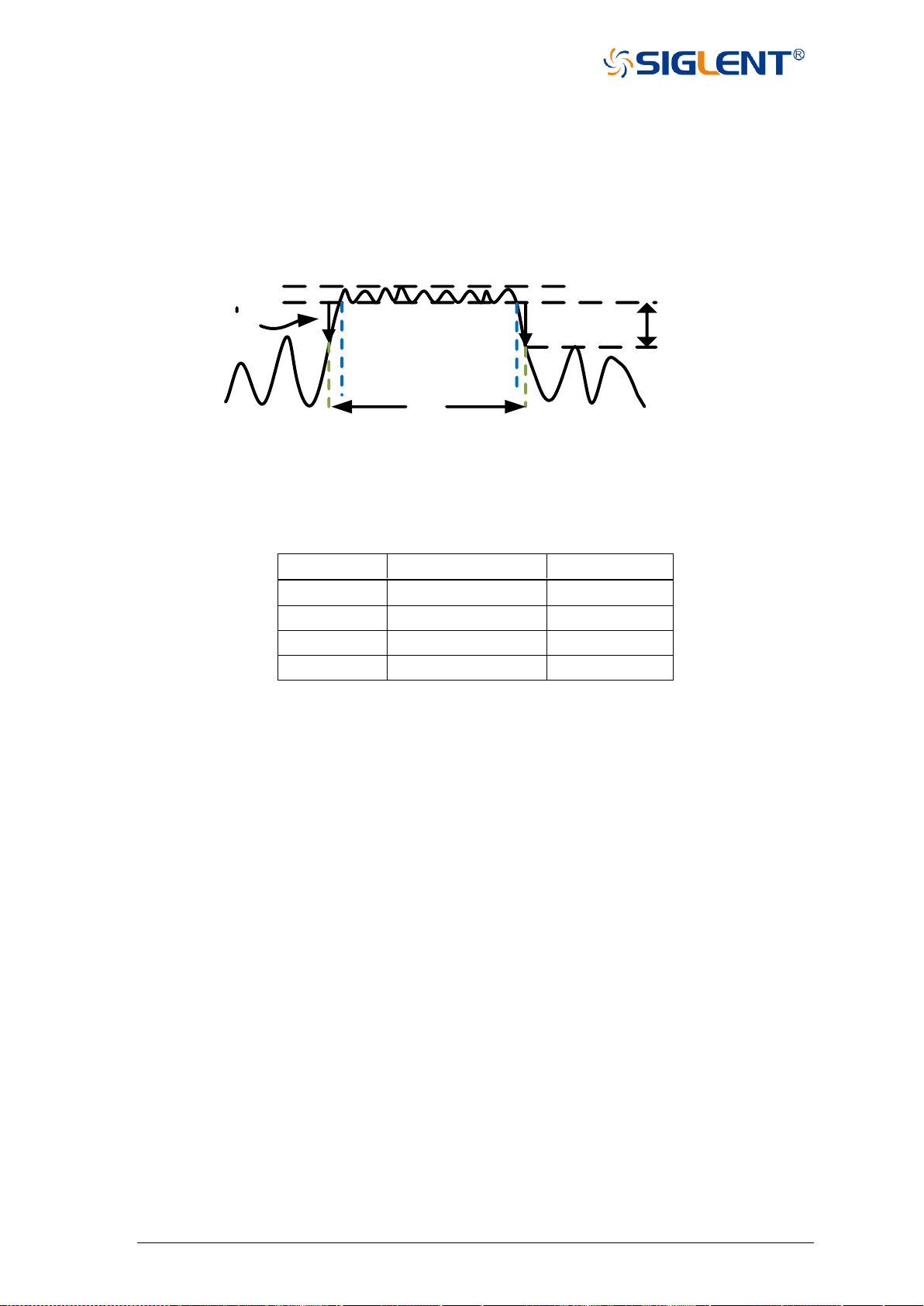
117 SNA5000A Vector Network Analyzer User Manual
⚫ Notch: Remove response using the gating span.
Gate shape: Set the filter characteristics of the gating function. There are four options:
minimum, normal, wide, and maximum.
The parameter definition of the gating function is shown in the figure below:
Bandwidth ripple
Sidelobe level
Gate shape
Gate marker
-6dB
T1
Gate start time
Gate stop time
Figure 4-13 Diagram of gating
Parameter description of gating function:
Gate shape
Bandwidth ripple
Sidelobe level
Minimum
±0.1 dB
-25dB
Normal
±0.1 dB
-45dB
Wide
±0.1 dB
-52dB
Maximum
±0.01 dB
-80dB
4.9.3 Window
There will be sudden changes in the start and stop of frequency domain parameter
measurement, which will lead to overshoot and ringing in the time domain. The window function
is helpful to reduce the overshoot and ringing in the process of frequency domain and time
domain conversion.
Click Math→Time Gating→Gating Setup→Window to open the window setting interface,
we can set the window size, The size of the window should be balanced between response
resolution and dynamic range. Setting the minimum window can get the best response
resolution, and setting the maximum window can get the maximum dynamic range.
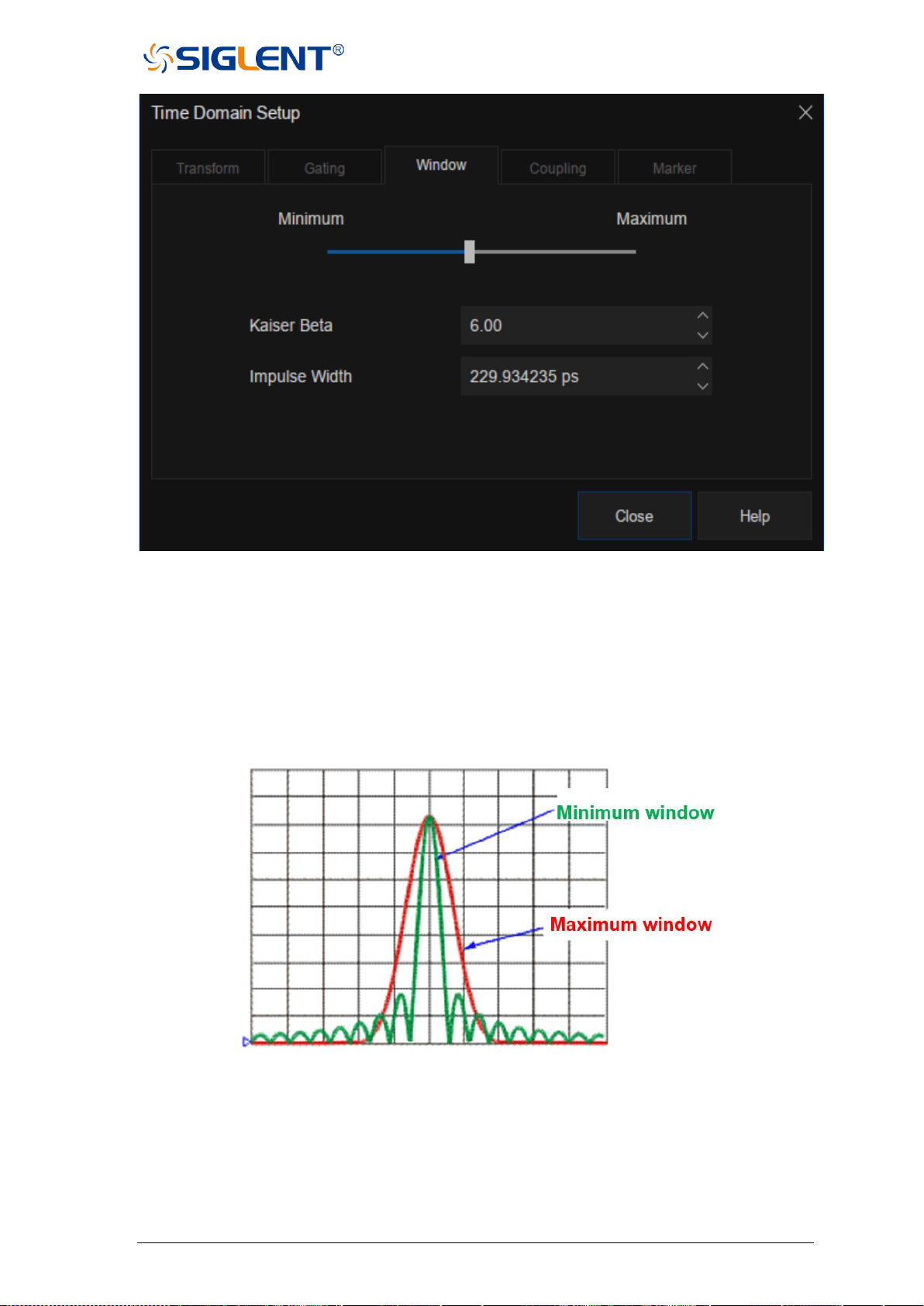
SNA5000A Vector Network Analyzer User Manual 118
Figure 4-14 Window setting interface
Three methods of setting window size:
⚫ Minimum-maximum: Use the mouse or touch screen to move the slider to
change the window size.
⚫ Kaiser Beta: Use the value of Kaiser Beta to change the window size.
⚫ Impulse width: Use the value of impulse width to change the window size.
Figure 4-15 Diagram of maximum and minimum window
4.9.4 Coupling
Trace coupling allows to change the measured time-domain parameters and make all other
measured parameters in the channel change the same. For example, to view the frequency-
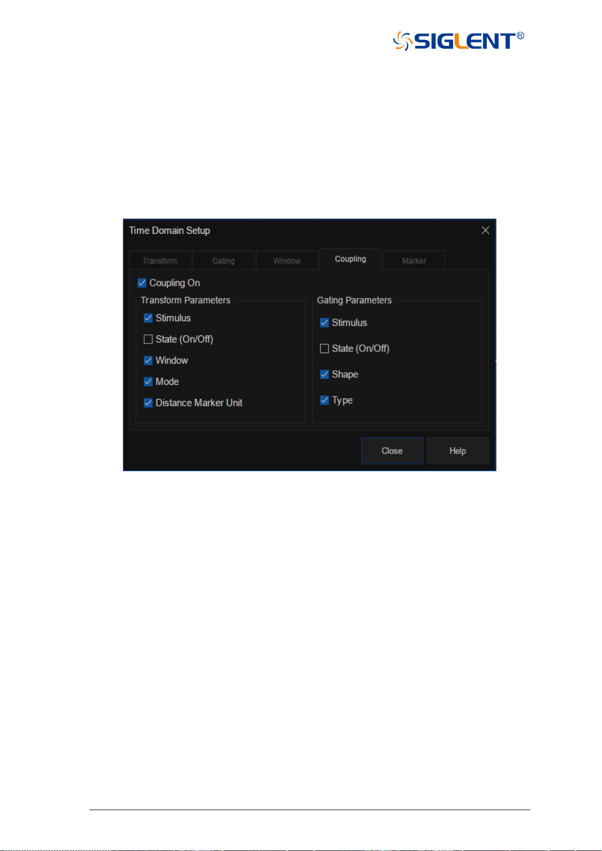
119 SNA5000A Vector Network Analyzer User Manual
domain and time-domain measurement parameters at the same time, first turn on the coupling
switch and select all the gating parameters in the coupling setting interface, at the same time,
the parameters of gate span are changed in time domain measurement, the frequency-domain
measurement parameters will be changed automatically to reflect the effect the time domain
gate span parameters are modified. The trace coupling is only applicable to Y-axis
scale/reference settings. The results of trace coupling do not change the measured data.
Click Math→Time Gating→Gating Setup→Coupling to open the coupling setting
interface, we can set transmission parameters and gating parameters in this interface.
Figure 4-16 Coupling setting interface
Coupling on: Click to enable coupling. At this time, all measurements in the channel are
coupled. The following conversion parameters and gating parameters can be
used for coupling.
Transform parameters:
⚫ Stimulus: Setting of the start time, stop time, center time, and span.
⚫ State(On/Off): State of the transform.
⚫ Window: Kaiser Beta and pulse width parameter.
⚫ Mode: Low pass pulse, low pass step, bandpass.
⚫ Distance marker unit: When selected, all measured distance marker units are
coupled.
Gating parameters:
⚫ Stimulus: Setting of the start time, stop time, center time, and span.
⚫ State(On/Off): Switch of gating function.
⚫ Shape: "Minimum", "normal", "wide" and "maximum".
⚫ Type: Bandpass and notch filtering.
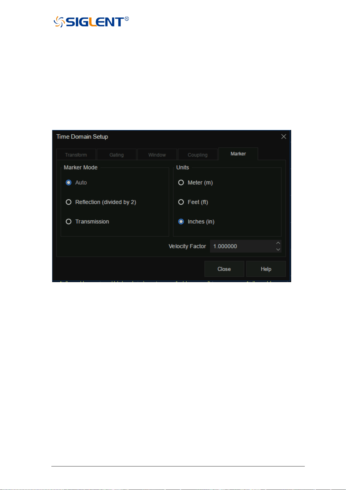
SNA5000A Vector Network Analyzer User Manual 120
4.9.5 Marker
When a marker is added to a time-domain parameter, the distance parameter is
automatically displayed in the marker reading. These settings only affect the display of all
markers of the active measurement (Unless the distance marker unit is coupled in the trace
coupling box).
Click Math→Time Gating→Gating Setup→Marker to open marker setting interface. Set
the marker mode, units, and velocity factor in this interface.
Figure 4-17 Marker setting interface
Marker mode: Specify the marker mode to determine the correct marking distance
displayed. Generally, Auto can be selected when measuring S parameter,
and Reflection or Transmission can be selected when measuring any
ratio parameter.
⚫ Auto: If the measurement parameter is S parameter, Reflection or Transmission will
be selected automatically. If the measurement parameter is a non-S
parameter, Reflection will be selected automatically.
⚫ Reflection: Displays the distance from the source to the receiver and the return path,
then divides by 2 (compensated return path).
⚫ Transmission: Displays the distance from the source to the receiver.
Units: Specifies the unit for the displayed marker distance value, there are three options:
meter, feet, inches.
Velocity factor: Set the velocity factor of the transmission line, where the value of PE is 0.66,
PTFE is 0.7 and the corresponding value of vacuum is 1.

121 SNA5000A Vector Network Analyzer User Manual
5 Guide For The TDR Option
5.1 Overview
Measured frequency responses can be transformed to the time domain to analyze the
time-domain characteristics of the DUT. The TDR option provides the time domain
reflection/transmission analysis functions and eye diagram simulation function, which can
help users save time and money by minimizing the need for other test equipment Time
domain analysis also has some irreplaceable advantages:
1. Time-domain analysis shows the positions and properties of the impedance
discontinuities on DUT. It can be easy to acquire the impedance value at any point on
the transmission line by analyzing the time domain reflection characteristics. It's
helpful to locate the faults on transmission lines.
2. Using the time domain gating function to remove the influences of the impedance
discontinuities, it becomes possible to simulate the frequency domain characteristics
of DUT after the faults are removed.
3. The eye diagram simulation function doesn't need any external waveform generators.
The VNA uses a built-in virtual bit pattern generator to provide the input signal. It's a
very important tool for signal integrality analysis.
4. If you want to design a compensation network for high-speed digital signal
transmission by emphasis/de-emphasis or equalization, the advanced waveform
function in TDR waveform will be of vital use for you. You don't need to change the
DUT connection or any extra devices, it's easy to simulate the eye diagrams with the
different compensation methods.
5. You can directly inject jitter into the input signal for eye diagram simulations. A
statistical eye diagram is introduced to simulate the probability density of the output
signals.
When using the TDR option, there are some notes:
1. When opening the TDR option or switching the DUT topology, calibration and deskew
data will be cleared. Please finish the calibration wizard before measuring to get the
correct results. Save the calibration data and recall it when required, which can avoid
unnecessary calibration operations.
2. Please operate in the bottom toolbar of the TDR menu as far as possible. The
function in the TDR option desends on the time domain transform, so changing
settings in the right toolbars can lead to incorrect transform results.
3. Don't close the eye diagram module while the eye diagram is drawing, or an
unexpected error might occur. Unless necessary, don't switch between the TDR/TDT
module and the eye diagram module, for the last eye diagram will be drawn when it's
switched to the eye diagram module, which might take a long time.
4. It's NOT recommended to add too many traces, or the trace data update will be slow.

SNA5000A Vector Network Analyzer User Manual 122
5. If there are too many windows or too much information in a window to observe the
information or traces, it will be useful to maximize the window or trace.
5.2 Open/Close/Preset TDR Option
To switch on the TDR option, use the order Math->TDR->TDR, then the button "On" will
be selected. The TDR toolbar will appear at the bottom of the screen, and the TDR option
function will be open to the user. If you have the trial license for the TDR option, an information
dialog will appear to notify you that the trial times will decrease. If the trial times expire, a
permanent license is needed to switch on the TDR option.
To close the TDR option, use the order Math->TDR->TDR again, then the button "Off" will
be selected, VNA will restore the state before the option opened. Click the button at the
top right corner of the TDR toolbar will close the TDR option, too.
Click the Preset button in the Basic bar of the Setup tab in the TDR toolbar and the VNA
will preset the TDR option: Clear the calibration data, allocate the traces and windows
automatically, and reset the settings in the option. After the TDR option is started, the
calibration wizard will need to be run again.
5.3 TDR Setup Wizard
The TDR setup wizard pops up when the TDR option is switched on for the first time. Click
the checkbox "Show this wizard next start-up" to decide whether the wizard pops up when
opening the option or not. The wizard can be opened by clicking the Setup Wizard button in
the Basic bar of the Setup tab in the TDR toolbar.
The wizard will guide you to finish the DUT topology selection, port extension setup, DUT
length measurement, and stimulus rise time setting. The calibration type can be selected in the
Error Correct bar on the first page of the wizard, and the wizard will also guide you to finish
the calibration you select. The calibration operation will be illustrated in detail in the section
"TDR calibration".
If you don't need to finish the setup in the wizard immediately, you can close the wizard.
But the calibration is necessary before accurate measurement or analysis.
5.4 Calibration for TDR Option
There are two calibration types in the TDR option: Deskew or Deskew & Loss
Compensation. The former only moves the reference plane to the end of the cables
connected to the ports of VNA, ignoring the signal loss in the cables. And the latter tries to
compensate the loss in the cables.
5.4.1 Deskew
Click the Deskew button in the Basic bar of the Setup tab in the TDR toolbar to open
the Deskew dialog. Connect all cables and fixtures to the VNA, and connect the other ends
123 SNA5000A Vector Network Analyzer User Manual
of the fixtures to nothing or the OPEN calibration kit. Then click the Deskew button in the
dialog, and click the Finish button after a mark appears at the Deskew button to finish
the Deskew calibration.
Click the Option button to open the Deskew Option dialog, in which you can select the
calibration type or operate the calibration one-by-one for each port. The calibration type can
be selected by the Standard Type pull-down menu. It's set to Open by default. If you choose
the Short option, you should connect the SHORT calibration kit to the port to finish the
calibration. You can calibrate only one port at a click on the corresponding Port button, but
you should finish the calibration of all ports to finish the task in the dialog.
5.4.2 Deskew & Loss Compensation
Click the Deskew&Loss button in the Basic bar of the Setup tab in the TDR toolbar to
open the Deskew & Loss Compensation wizard. The wizard can be divided into 3 steps,
which guide you to finish the Deskew and Loss Compensation calibration.
At the first step, a Deskew calibration is required. The method is the same as the
operation introduced in the section "Deskew".
At the second step, the calibration operation depends on the correct DUT topology.
Under the topology Single-Ended 1 Port, you need to connect the cables and fixtures to the
VNA, connect the other ends of the fixtures to nothing or an OPEN calibration element. Click
the Measure button in the wizard, wait for the mark to appear at the Measure button to
finish the second step of calibration. Under other DUT topologies, you need to connect two
cables and fixtures, which are connected to the ports as the wizard instructs, to both ends of
a THRU calibration kit. Click the Measure button in the wizard, wait for the mark to
appear at the Measure button, then execute the next operation. If under Single-Ended 4-Port
or Differential 2-Port, you will need to execute the operation as stated above once for each
page of the wizard respectively to finish the second step.
At the third step, you can connect the LOAD calibration element to every port, and click
the corresponding Port button to execute the calibration step. The step is optional, so it's not
necessary to finish the calibration wizard.
If you finish all necessary calibration operations, click the Apply button to save and apply
new calibration data, and click the Finish button to close the wizard.
At any step of the wizard, it's allowed to execute a calibration operation repeatedly, new
measured data will replace original data. You can click the Close button to close the wizard,
which will give up all data measured in the wizard unless you have clicked Apply button to
save them.

SNA5000A Vector Network Analyzer User Manual 124
5.5 TDR Channel Setup
When the TDR function is activated, the current state is saved, and all existing traces
and channels are deleted, and a new channel is added for the option. When the option is
closed, all traces and the channel being used are deleted, and the instrument is returned to
the state before TDR was opened.
The current channel settings can be changed in the TDR toolbar at the bottom of the
screen, usually in the Setup tab.
5.5.1 DUT Topology
In addition to the Setup wizard, the DUT topology can be changed in the DUT topology
pull-down menu in the Basic bar of the Setup tab. The traces and windows are allocated
automatically according to the DUT topology.
If the DUT topology is changed, the calibration and deskew data will be cleared.
Recalibration becomes necessary before an accurate measurement or analysis. If the
calibration data is hoped to be held, save the state in time and recall it when required.
5.5.2 DUT Length
The DUT length means the time that the signal takes to transmit through the DUT or
reflect the incident plane and is required to show the time-domain responses of DUT in full.
The sweep frequency span and points of the channel are set according to the DUT length,
and the span of the transformation is automatically calculated by the DUT length when the
time domain traces are set in the time axes. It's not recommended to change the sweep
settings by other methods.
In addition to the Setup wizard, the DUT length can be set in the DUT Length textbox in
the Basic bar of the Setup tab. It's a convenient way to set the suitable value by measuring
the DUT length in the DUT Length dialog. Click the Auto button on the left of the textbox to
open the dialog, connect the DUT according to the picture and instructions in the dialog, click
the Measure button and wait for the mark to appear, click the Finish button to close the
dialog, and finish the DUT length setting. If the measurement result is out of the default
range, an information dialog will pop up to notify the users that the DUT length will be set to
the maximum or minimum.
5.5.3 Stimulus Magnitude in Time Domain
The stimulus magnitude in the time domain can be set in the Stim. Ampl. textbox in the
Basic bar of the Setup tab, which defines the magnitude of the impulse or step stimulus
signal for the time-domain responses of the traces under the format Volt.
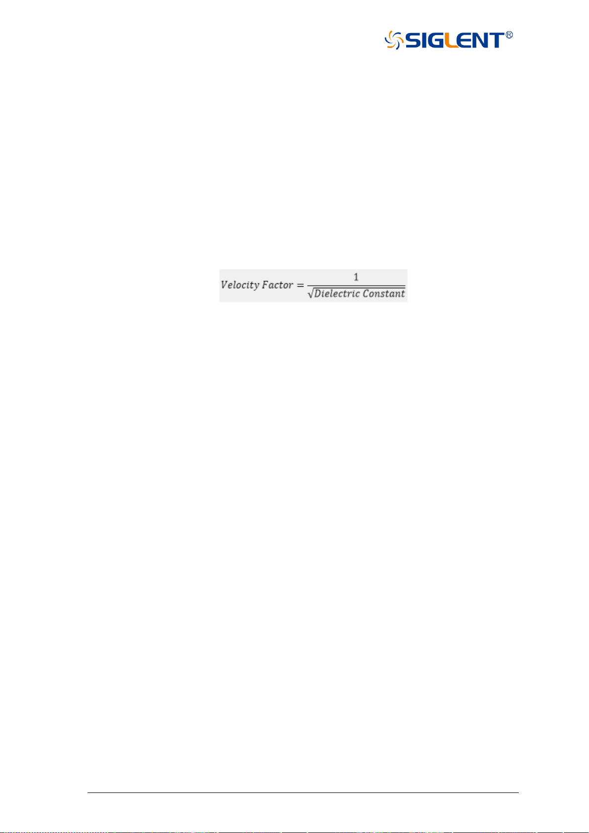
125 SNA5000A Vector Network Analyzer User Manual
5.5.4 Port Impedance
The port impedance can be set in the Ref. Z textbox in the More Function bar of the
Setup tab, which defines the reference impedance to calculate the impedance values of the
traces under the format Impedance.
5.5.5 Velocity Factor & Dielectric Constant
The velocity factor is the ratio of the velocity of the electric signal in the DUT to that in
the vacuum. VNAs calculate the distances by the transmission or reflection time based on
this factor, which provides the accurate positions of the impedance discontinuities. There is a
functional relationship between the velocity factor and the dielectric constant of the materials.
When either is changed, the other will be calculated by the equation below:
The velocity factor and dielectric constant can be set in the Velocity Factor and
Dielectric Const. textboxes in the More Function bar of the Setup tab.
5.5.6 Power Level
The power level is the power of the test signal transmitted to the DUT, which can be set
in the Source Power spinbox in the More Function bar of the Setup tab.
5.5.7 Average
The average function means that the final measure results are equal to the average of
the measure results in the several sweeps in the same setting, and the number of sweeps
needed depends on the averaging factor. The average function can decrease the random
errors to some degree, but slow down the update of trace data. It's necessary to keep the
characteristics and connection of the DUT unchanged during an average sweep.
To enable or disable the average function, click the Averaging checkbox in the Average
tar of the Setup tab. The average factor can be set in the textbox to the right of the
checkbox.
5.5.8 IF Bandwidth
The IF bandwidth is the bandwidth of the intermediate-frequency filters in the receivers.
A narrow IF bandwidth leads to lower trace noise levels and longer sweep times.
The IF bandwidth can be set in the IF Bandwidth textbox in the Average tar of the
Setup tab.
5.5.9 Trigger Mode
The trigger mode gates the channel sweep state change when the trigger signal is
detected. The trigger mode Hold/Stop means that sweep can't be started even if the trigger
signal is detected. Single means that only one sweep is triggered by the trigger signal. Upon

SNA5000A Vector Network Analyzer User Manual 126
sweep completion, the trigger mode is set to Hold/Stop. Continuous/Run means that the
trigger signal starts and continuously sweeps.
To switch the trigger mode to Continuous/Run, click the Run button at the top of the
TDR toolbar. To switch the trigger mode to Single, click the Stop/Single button at the top of
the TDR toolbar.
5.6 TDR Trace Setup
Without taking the set coupling into account, the settings as follows are applied to a
single trace. Usually, the traces in the TDR option are in a time-domain coupling and marker
coupling, meaning that the correlated settings are applied to all the traces. In addition, There
is a set of default trace configurations for every DUT topology.
5.6.1 Select a Trace
In addition to clicking the trace or trace information bar on the screen, the Trace pull-
down menu at the top of the TDR toolbar has the same function.
5.6.2 Scale Management
In the TDR option, there are several automatic scale settings to use, and it is allowed to
change the scale or reference value manually.
5.6.2.1 Auto Scale
To apply the automatic scale settings, click the Auto Scale button at the top of the TDR
option and click the suitable option in the pull-down menu. Every option in the menu
represents a set of automatic scale settings.
Option X means that the horizontal axis of the current trace is set automatically. For the
traces in the time domain, the scale and reference value are calculated by the DUT length.
For the traces in the frequency domain, the horizontal axis is set to the frequency sweep
setting of the channel.
Option Y means that the vertical axis of the current trace is set automatically. The scale
and reference value are calculated by the maximum and minimum of the trace data.
Option X&Y means that the horizontal and vertical axes of the current traces are set
automatically. The method is the same as introduced above.
All Trace means that the horizontal and vertical axes of all the traces are set
automatically. The method is the same as introduced above.
5.6.2.2 Manual Scale Setup
Manual scale setting is in the Horizontal and Vertical bar of the TDR/TDT tab. There
are two sets including a scroll-wheel and a textbox, the left set is used to change the scale
values, and the right one is for the reference values. The reference position of the horizontal
axis can be changed by the or button between two scroll-wheels in the Horizontal

127 SNA5000A Vector Network Analyzer User Manual
bar: The first scale line on the left or the center scale line. The reference position of the
vertical axis is the center scale line by default.
The vertical axis of the traces in the frequency domain has no concern with the sweep
setting of the channel, only to set the displayed span of the trace data.
5.6.3 Memory Trace Management
Memory trace management is in the Data/Mem pull-down menu at the top of the TDR
toolbar. Click the Data->Mem order in the menu, and the current trace data is saved to the
memory trace. Other orders in the menu are display modes of the data trace and the memory
trace for the current trace: The option Off means the data trace and the memory trace are
invisible. The option Memory means only the memory trace shows in the window. The option
Data means only the data trace shows. The option Data&Mem means both of them are
visible.
5.6.4 Measure Parameter & Format
The measurement parameters and formats of the traces can be set in the Parameter tar
of the TDR/TDT tab.
The physical significance of measurement parameters and formats in the frequency
domain is the same as the general parameters of the VNA. In the time domain, T parameters
are used as measurement parameters, meaning that the ratio of the magnitudes of the
response signals received to the stimulus signals when a unit step/impulse stimulus signal is
transmitted to DUT at time zero, in a span. For a specified DUT, S parameters are functions
of the signal frequency, while T parameters are functions of the time under a specified
stimulus type. T parameters show the unit step/impulse response of the DUT, which is of vital
importance in the time domain system analysis.
The formats of T parameters include Log Mag, Lin Mag, and Real, which are the same
as S parameters; moreover, Impedance and Volt are added. T parameters show the time
domain responses, so the values are always real numbers. In the other words, the imaginary
parts are always zero. Therefore, Imaginary or phase formats aren't provided for T
parameters in the TDR option. The magnitude of Log Mag and Lin Mag formats is
intrinsically the absolute values of the real parts of T parameters.
Impedance format is usually used for the reflection T parameters under a unit step
stimulus. It calculates the impedance value of each point in the signal transmitting path by
the reflection T parameters (reflection coefficients) under the unit step stimulus, which is on
the base of the port impedance. The distances are calculated by the delay of transmission
and the velocity factor. In the Impedance format, the positions and properties of impedance
discontinuities in the DUT are shown on the traces visually, which provides a piece of
important information for fault detection and removal. In the Impedance format, the TDR
option regards the T parameters as the reflection coefficients ρ, and calculates the
impedance by the equation as follow:
Volt format means the trace shows the time domain waveform of the response signal
received under the specified stimulus. The magnitude of the stimulus signal is defined by the

SNA5000A Vector Network Analyzer User Manual 128
value in the Stim. Ampl. textbox in the Basic bar of the Setup tab. Intrinsically, the Volt format
means the trace data is a product of the T parameters and the magnitude of the stimulus signal.
Click the measure parameter button in the grids on the left of the Parameter bar, the
measurement parameter of the current trace switches to the corresponding parameter. To
switch on or off the time domain transform of the current trace, click the pull-down menu in the
left of the Measure line. To switch to balance or unbalance parameters, click the pull-down
menu in the right of the Measure line. To change the format, click the Format pull-down menu.
5.6.5 Stimulus in Time Domain
The stimulus type can be set in the Stimulus pull-down menu in the Parameter bar of
the TDR/TDT tab. There are two stimulus types to choose: The option Lowpass Step means
T parameters show the unit step responses and the option Lowpass Impulse means T
parameters show the unit impulse responses.
The rise time or impulse width of the stimulus signal can be set in the Rise Time or
Impulse Width textbox. Intrinsically, it controls the beta value of the Kaiser window function
applied in the time domain transformation to weaken the sidelobes. Because the
transformation is based on the finite frequency domain data, the data truncation at the end of
frequency domain data leads to some problems, such as the extension of the rise time or
impulse width of the responses signal and the appearance of sidelobes, which is called
"truncation effect". Applying the Kaiser window lowers the sidelobe levels, but aggravates the
extension of the rise time or impulse width and brings down the resolution ratio of
transformation. The longer the rise time or impulse width of the stimulus signal, the larger the
beta value of the Kaiser window function, the stronger effects explained above are introduced
into the transformation.
5.6.6 Smoothing
The smoothing function makes the trace data smooth by replacing the original trace data
with the average of the data nearby. If the local change ratios of trace data are relatively
large, the smoothing leads to large data errors. Therefore, the smoothing function is available
for the traces whose measure parameters are reflection S parameters.
To switch on or off the smoothing function, click the Smoothing checkbox in the
Parameter bar of the TDR/TDT tab.
5.6.7 Trace Allocation
The TDR option will delete all existing traces and windows, allocate all the traces and
windows automatically for the DUT topology, and set the traces to default settings if the trace
allocation function is activated. The operation deletes all original traces and their settings, but
the channel settings remain. There are three allocation methods to choose from: The option
Mixed means that the traces in the time and frequency domain are allocated. The option All
T means that only traces in the time domain are allocated. The option All S means only
traces in the frequency domain. Note that in Single-ended 1 Port topology, only the option
Mixed is available.
To use the trace allocation function, click the button of the corresponding method in the
Allocation box in the Trace Control bar of the TDR/TDT tab.

129 SNA5000A Vector Network Analyzer User Manual
5.6.8 Trace Setup Coupling
To switch on or off the time domain or marker coupling, click the Time domain or
Marker checkbox in the Coupling box in the Trace Control bar of the TDR/TDT tab.
5.6.9 Time Domain Gating
The time-domain gating function transforms the time domain response into the
frequency domain after removing a part of the response. Usually, the function is used to
simulate the expected frequency domain response after removing some faults by removing
the abnormal responses resulting from the impedance discontinuities. The operation
procedure includes enabling the time domain transformation, setting the parameter to
remove partial time-domain responses, observing the other traces in the frequency domain
whose gating settings are coupled with the trace, or close the time domain transformation to
observe the frequency responses.
The time-domain gating settings in the TDR option can be changed in the Gating bar of
the TDR/TDT tab.
To switch on or off the time domain gating function, click the Gating checkbox.
To change the function type of the gating range, click the ratio button in the Type box.
The option Notch means that the responses in the gating range will be ignored, while the
option Bandpass means that the responses beyond the gating range will be ignored.
The scroll-wheel and textbox can be used to change the start and stop position of the
time domain gating range.
5.7 TDR Data Analysis & Output
The general marker search function is available in the TDR option for data analysis, and
there are some shortcuts provided at the top of TDR toolbar for marker management and
search for maximum/minimum with tracking. In addition, the functions of the rise time search
and delta time search are introduced as the time domain trace data analysis tools in the TDR
option.
To correct the errors of impedance calculation resulting from the complicated distribution
of mismatches in the DUT, a peeling algorithm is introduced to reveal the actual impedance
value of every point on the passive DUTs.
The shortcuts to save/recall the state files, output the trace data to the files, and save the
screenshot are provided in the File pull-down menu at the top of the TDR toolbar.
5.7.1 Marker Setup
In addition to the general ways to manage the markers in the VNA, the Marker pull-down
menu at the top of the TDR toolbar is a way to add or delete markers.
The order in the first group of the Marker Search pull-down menu is shortcuts to
manage the common marker tracking marker. The option Off closes the search function of
the current marker, while the Max or Min starts the tracking search for maximum or
minimum.

SNA5000A Vector Network Analyzer User Manual 130
5.7.2 Rise Time Search
Rise time search is only available for the trace in the time domain, which searches for
the rising or falling edge, sets a label to the start and stop, and displays the transition type
and time at the top left corner of the window if successful. It's a tracking search, the results
update if the trace data changes.
To switch on or off the rise time search, click the Rise Time(10-90%) or Rise Time(20-
80%) option in the Marker Search pull-down menu. Selecting the suitable search type
depends on the requirements.
5.7.3 Delta Time Search
Delta time search is only available for the trace in the time domain, which searches for
the difference between the time where two traces rise or fall to a specified relative level in
respective transition edge. If successful, a label will be set to the relative level on both traces,
and the results will be displayed at the top left corner of the window that contains the start
trace of the search. It's a tracking search, the results update if the trace data changes.
Click the △Time... order in the Marker Search pull-down menu to open the △Time
dialog, and the settings of delta time search can be changed here.
Click the Trace(Start) pull-out menu to change the start trace of the search, click the
Trace(Stop) pull-out menu to change the stop trace. A trace in the time domain can start one
search at most as a start trace, while it's allowed that more than one searches set the same
trace as the stop trace.
The target relative level of the search can be set in the Position(%) textbox in the
dialog.
To switch on or off the search, click the △Time Enable checkbox.
5.7.4 Peeling
If there are two or more impedance mismatches on the DUT, a part of the incident wave
is reflected at the first mismatch, the incident energy arriving at the next mismatch reduces,
so the reflection at the next mismatch might seem weaker than that in reality. Calculating
impedance using reflection coefficients might lead to obvious errors after the first mismatch.
To avoid the effect of the masking phenomena explained above, a new approach to calculate
impedance, called the peeling algorithm, is introduced in the TDR option. The algorithm
divides the DUT into many sections, calculates the impedance of the next section by the
impedance of the last section as the reference value, and the incident and reflected energy in
reality.
The algorithm presupposes that the energy sum of input equals that of output at any
points on the path the signal transmits through, which means that the signal transmits
through the DUT without loss. This is an imperfection of the algorithm, and transmission loss
always decreases the accuracy. Because of the recurrence method in the algorithm, the
accuracy also decreases with the distance increases.
If the peeling function is enabled, the TDR option calculates impedance in the way
explained above, instead of the traditional way. The function is available only if the format of

131 SNA5000A Vector Network Analyzer User Manual
the trace is Impedance of the reflection T parameters. To switch on or off the function, click
the Peeling checkbox in the Parameter bar of the TDR/TDT tab.
5.7.5 File & Data Output
In the File pull-down menu at the top of the TDR toolbar, there are some shortcuts for file
operation and data output.
The order Save State... is used to save the current state and calibration data as a ..CSA
file, and Recall State... is used to restore them from the files.
The order Save Trc Data... is used to save the current trace data to .CSV file, and Save
SnP... saves all available S parameters data as an .SNP file whose format depends on the
DUT topology.
Screenshot... is used to save the screenshot as a .PNG file.
5.8 Eye Diagram Simulation
5.8.1 Overview
Eye diagrams are used to analyze the influence of the intersymbol interference and
noise on transmission performance, which is an important tool for signal integrity analysis.
The eye diagram simulation function, included with the TDR option, is built on a virtual digital
signal generator and the frequency characteristics of the DUT. It simulates that a virtual input
digital signal transmits through the DUT, and analyzes the output signal to get an eye
diagram. This is different from the traditional way of using an oscilloscope to draw eye
diagrams. There is no need to provide an external digital signal to the input port of the DUT.
To simulate different input signals, change the stimulus settings in the eye diagram module.
The data analysis of eye diagrams in the option will try to get the numerical
characteristics of the diagram and mark them on the diagram if required, which is designed to
help the users obtain the key information quickly.
The jitter injection and statistical eye diagram function are provided to analyze the
influence of the jitter in the input signal on the transmission performance.
The mask test on the eye diagram and preinstalled mask patterns are a convenient
method of estimating whether the eye diagram meets the design requirements.
To start an eye diagram simulation after completing the simulation settings, click the
Draw Eye button in the Trigger box of the Eye/Mask tab.
5.8.2 Stimulus Bit Pattern
There are 3 bit pattern types to choose in the option: Pseudo-Random Binary Sequence
(PRBS), K28.5 comma code, and the user's bit pattern.
For more information about PRBS, refer to the section Bit Pattern Length. K28.5 comma
code is defined in an industry-standard developed by IBM which includes comma (control)
characters. The user's bit pattern is imported from the user-defined files. The introduces of the
bit pattern types in the table as follow:

SNA5000A Vector Network Analyzer User Manual 132
Type
Bit Pattern Length
Generator
PRBS
Depends on the users,
limited in 2
n
-1, n = 3,5,7,9,11,13,15
Generated by a virtual PRBS generator
K28.5
20
"00111110101100000101" (20 bits)
User
limited between 2 and 8192
Imported from a user-defined file
5.8.2.1 Bit Pattern Type
To change the input bit pattern types, click the Type pull-down menu in the Stimulus box
of the Eye/Mask tab.
The option Statistical in the menu is used to switch on the statistical eye diagram mode,
which cannot change the bit pattern types for the normal eye diagram simulation.
5.8.2.2 Bit Pattern Length
The bit pattern length of K28.5 code is 20 bits, and that of the user pattern depends on
the text in the file. Only the length of PRBS can be changed in the eye diagram simulation
module by clicking the Length pull-down menu in the Stimulus box.
A set of Linear Feedback Shift Register (LFSR) is simulated to generate virtual PRBS,
whose maximum period is selected to equal the bit pattern length. The maximum of the period
of PRBS, generated in a set of LFSR of n level, is 2
n
-1. In the other words, in ideal conditions,
the sequence will iterate all possible binary numbers of n bits. The initial condition of the LFSR
is random, PRBS generated becomes random to find the worst bit pattern of n bits for
transmission performance. Eye diagram simulation always includes all n-bit input patterns to
show the worst transmission performance of DUT, if PRBS is set as the input signals. So it's
recommended to use PRBS as a bit pattern to draw eye diagrams.
The bit pattern length of PRBS is limited in 2
n
-1, and n = 3, 5, 7, 9, 11, 13, 15. That means
the bit pattern will be generated by LFSR of n level, to include the worst condition as far as
possible. The larger length is selected, the degree of the simulation perfection for intersymbol
interference becomes better, but running time becomes longer.
5.8.2.3 User Pattern
If the eye diagram is required to simulate the specific bit pattern as the input signal, select
the option USER in the Type pull-down menu, and click the User Pattern button to open the
Bit pattern Editor dialog to set the user-defined pattern. In the dialog, you can load .txt files
to import the text as the bit pattern and edit the bit pattern in the textbox. Close the dialog after
loading or saving the bit pattern file, the pattern will be used for the next eye diagram simulation.
The text file to load must contain 0 and 1, but any other characters; and the length of text
must be between 2 and 8192.

133 SNA5000A Vector Network Analyzer User Manual
5.8.3 Stimulus Signal Setup
5.8.3.1 Logic Level
To change the logic level of the input signal, set the value in the One Lv. or Zero Lv.
textbox in the Stimulus box.
5.8.3.2 Data Rate
The data rate of the signal is the number of bits transmitted per second, which reflects the
base frequency of the signal. Considering the lowpass characteristics of transmission systems
in reality, the transmission becomes bad with a large data rate, and the signal integrity analysis
becomes important.
To change the data rate of the input signal, set the value in the Data Rate textbox in the
Stimulus box.
5.8.3.3 Rise Time
The rise time of the signal reflects the steepness of the transition edge. The smaller rise
time means the higher degree of steepness, the larger proportion of high-frequency parts, and
the more serious high-frequency losses can be during transmission. It's effective to widen the
eye by reducing the rise time properly. But too small a rise time leads to ringing phenomena at
the logic level of the output signal, resulting in the decrease of the eye height.
To change the rise time type or value of the input signal, operate the Rise Time pull-down
menu or textbox in the Stimulus box.
5.8.4 Eye Diagram Analysis
During the eye diagram simulation, the option analyzes the eye diagram automatically
and try to get the numerical characteristics as follow: Rise Time, Fall Time, Jitter, Crossing
Percent, Opening Factor, The Ratio of Signal to Noise, Duty Cycle Distortion, Level
One, Level Zero, Level Mean, Amplitude, Height, Width. And Rise Time, Fall Time, Jitter
(peak-peak value), Amplitude, Height, Width are allowed to be marked on the eye diagram
to conveniently obtain the characteristics of the eye diagram.
5.8.4.1 Analysis Result Overlay
To switch on or off the data analysis markers on the diagram, click the Overlay checkbox
in the Result bar.
5.8.4.2 Rise Time in Data Analysis
To change the rise time type for data analysis of eye diagrams, click the Rise Time Def.
pull-down menu in the Result bar.

SNA5000A Vector Network Analyzer User Manual 134
5.8.5 Eye Diagram Scale Management
By default, the eye diagram is displayed in the automatic scale settings, which show the
details as clearly as possible. They can also be manually changed.
The scale settings in the vertical axis can be changed manually. But those in the
horizontal axis depend on the data rate of the input signal, which can't be changed after the
simulation starts.
To switch to a scale setting mode, click the Auto Scale or Manual radio button in the
Scale/Mask bar.
To change the scale or offset values in Manual scale mode, set the value in the
Scale/Div or Offset textbox. The Offset value here is the value that the center vertical scale
line refers to.
5.8.6 Mask Test for Eye Diagram
Mask patterns are some areas where the eye diagram is forbidden to pass, which
transfer the design requirements of the transmission systems into the numerical
characteristics of eye diagrams. They usually rule the tolerance of logic 0,1 level and rise or
fall time. If the eye diagram passes through the areas, the TDR option judges that the eye
diagram can't meet the requirement, leading to the failure of the mask test. According to
different communication standards, or at the different nodes in a communication system,
different mask patterns should be applied. The first step to mask test is to select or design a
suitable mask pattern based on the requirements.
To select or change the mask pattern applied, click the Mask Pattern button in the
Scale/Mask bar to open the Mask Pattern dialog.
In the File tab of the dialog, preinstalled standard patterns or user-defined mask files
(.MSK format) can be loaded. In the Scale tab, the Margin of the mask, start Position of a
bit, Delta time of a bit, and Logic Level can be set in textboxes. In the Edit tab, the positions
of vertices in the mask pattern can be changed by set values in the textboxes. Dragging the
vertices in the left window also makes sense, but it's recommended to drag with a mouse
connected to the VNA, because the points may be too close together for easy entry using
touch operation.
Close the dialog after saving the modifications to a mask file, the new pattern will be
applied to the next mask test.
To switch on or off the mask test, click the Mask Test checkbox in the Scale/Mask bar.
5.8.7 Jitter & Statistical Eye Diagram
Jitter is the transient deviation from the corresponding ideal position of a signal over
successive trigger events. High jitter worsens the transmission performance. It's divided into
the Deterministic Jitter (DJ) and the Random Jitter (RJ). RJ is generated by some
unpredictable factors and is independent of the input bit patterns. The models for RJ usually
have a Gaussian distribution, and the magnitudes are represented in root mean square
(RMS) values. DJ is generated by some repeatable and predictable factors and usually has a
finite magnitude value. The jitter related to the input bit patterns in DJ is called the Data
Dependent Jitter (DDJ), while the other jitter in DJ is called the Periodic Jitter (PJ).

135 SNA5000A Vector Network Analyzer User Manual
To change the settings of the jitter injection, click the Advanced Waveform button in the
Stimulus box of the Eye/Mask tab, or click the buttons in the Adv Waveform bar of the
Setup tab, to open the Advanced Waveform dialog. Click the Jitter button at the top of the
dialog to switch to enter the jitter setting interface.
To change the jitter type injected into the input signal, click the Random or Periodic
ratio button in the Type box. To set the jitter parameters, set the values in the corresponding
textboxes.
To select the jitter magnitude units, click the Jitter Unit pull-down menu. The unit UI
means that the time difference value between the zero time of two adjacent transition edges
in the signal, which is the default jitter magnitude unit.
To set the probability limit to display in the statistical eye diagram, click the Display
Limit pull-down menu. If the probability of the signal appearing is lower than the display limit,
it will be ignored and set to zero in the statistical eye diagrams.
To switch on the jitter injection for the next simulation after completing the jitter settings,
click the Enable checkbox in the jitter setting interface. When the jitter injection function is
switched on, the statistical eye diagram mode is enabled at the same time, the input bit
pattern type is switched to Statistical.
To switch to the statistical eye diagram mode in manual, select the option Statistical in
the Type pull-down menu in the Stimulus box. In the statistical mode, the input bit pattern is
set to PRBS with a fixed length, so the statistical eye diagrams might be slightly different in
several simulations of the same settings. The probabilities are represented by colors in the
statistical eye diagrams: Warm colors indicate a large probability, red represents the largest
ones; cold colors indicate a small probability, with deep blue representing the smallest
values.
5.9 TDR Advanced Waveform Function
The Advanced waveform function is applied in both modules of the TDR option,
TDR/TDT analysis, and eye diagram simulation, which includes viewpoint setting,
emphasis/de-emphasis, de-embedding, and Continuous Time Linear Equalization (CTLE).
The corresponding settings in the Advanced Waveform dialog, which can be opened by
clicking the buttons in the Adv Waveform bar of the Setup tab or the Advanced Waveform
button in the Stimulus box of the Eye/Mask tab.
To switch the dialog to the interface for setting the specified function, click the
corresponding button at the top of the dialog.
5.9.1 Viewpoint
To switch the viewpoint of the waveform to stimulus or responses, click the
corresponding View ratio button at the top of the dialog.
Click the ratio button before the DUT icon, switch the viewpoint to stimulus, and the
trigger mode is set to Hold/Stop, the transmission parameters show the stimulus signal only
processed by emphasis/de-emphasis, which is the signal transmitted to the DUT. Setting the
trigger mode to Continuous/Run, the viewpoint will be set to responses automatically.

SNA5000A Vector Network Analyzer User Manual 136
Click the ratio button after the DUT icon, switch the viewpoint to responses, and set the
trigger mode to Continuous/Run. The transmission parameters show the responses
processed by emphasis/de-emphasis, DUT, and equalization.
5.9.2 Emphasis/De-emphasis
Because of the lowpass characteristics of transmission systems, the high-frequency
components in the signal have higher losses than those at lower frequencies and the
phenomenon becomes more serious as the transmission distance increases. The
phenomenon is the main contributor to signal distortion during transmission. To control this
distortion, the emphasis/de-emphasis technology is introduced to compensate for these
additional losses by increasing the relative levels before the transmission. Transition edges in
the time domain represent high-frequency components in the frequency domain.
Emphasis/De-emphasis technology is designed to increase the level variation of the edges
by adjusting the levels of the bits close to the edges. The parameters to adjust the levels of
the first bit before or after the edges, and those for the two bits after the edges, are provided
in the TDR option and are defined as Pre Cursor, Post 1 Cursor, Post 2 Cursor. By changing
these parameters, it's easy to simulate the influence of the different emphasis/de-emphasis
strategies on the transmission performance in eye diagram simulations.
To change the parameters, set the value in the textbox in the Emphasis interface, and
click the Enable checkbox to enable the function. The function is available in transmission
parameters measurement and eye diagram simulations.
5.9.3 Equalization
To control the signal distortion resulting from the additional loss of high-frequency signal
components, equalization technology is introduced to amplify the high-frequency parts
properly after receiving the signal to balance the loss over variousfrequency spans. A
highpass filter and a continuous-time linear equalizer (CTLE) can be implemented. The CTLE
simulation function in the TDR option allows the user to adjust the system function of the
equalizer, to simulate the inflence of the equalization on the transmission performance in eye
diagram simulations.
To change the system function, set the value in the textbox in the Equalization interface, and
click the Enable checkbox to enable the function. The function is available in transmission
parameters measurement and eye diagram simulations.
6 Guide For The SA Option
6.1 Overview
Spectrum Analysis function is based on the VNA hardware, by adjusting the local oscillator
signal and mirror suppression algorithm processing to obtain the signal spectrum, so as to
achieve spectrum analysis function.
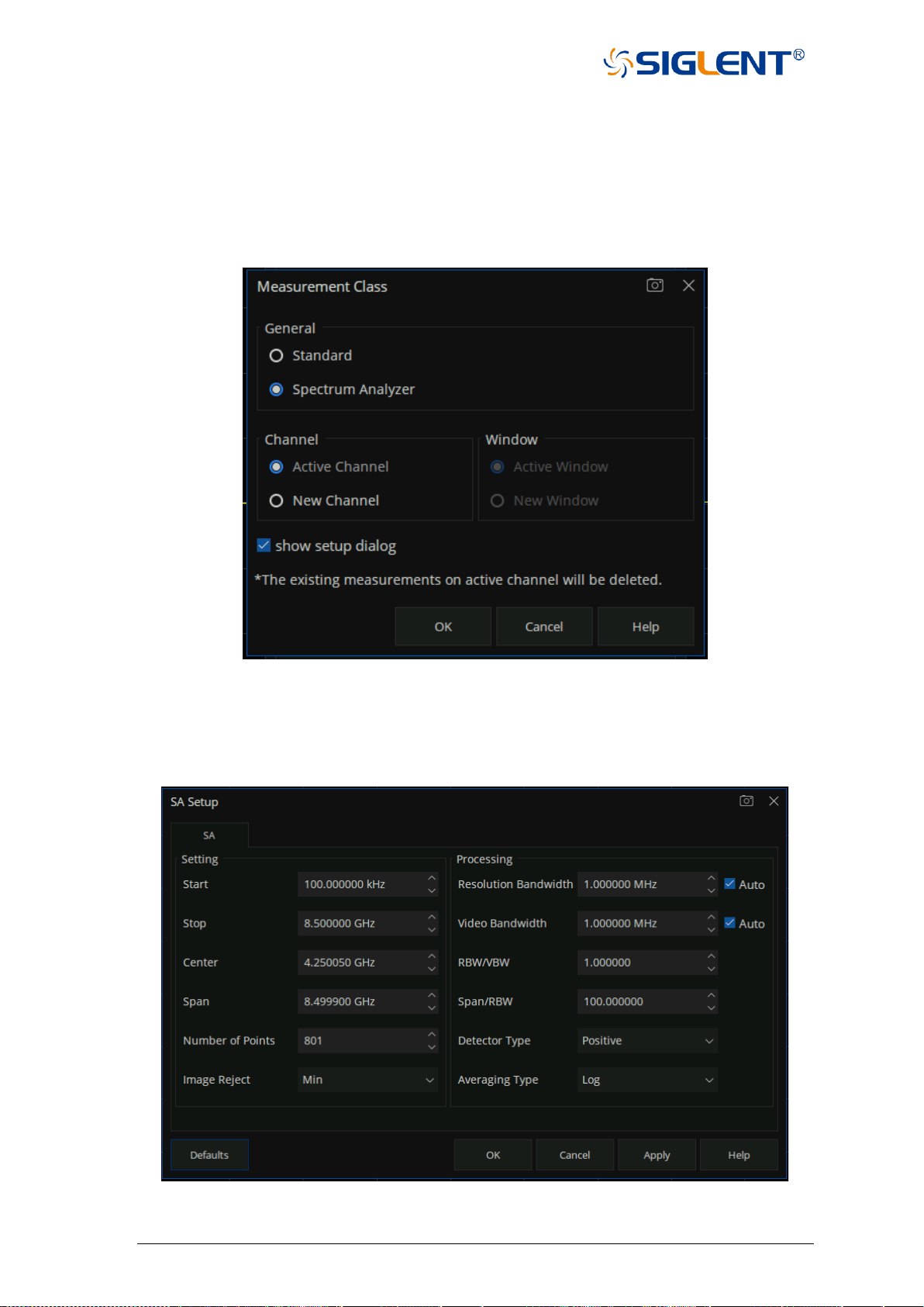
137 SNA5000A Vector Network Analyzer User Manual
6.2 Create a Spectrum Analysis Channel
Press “Meas “on the front panel , click S-Params > Other… > Measurement Class to open the
Measurement Class dialog box. Select Spectrum Analyzer, then either click Active Channel
(delete the existing measurement ) or New Channel then click OK. A Spectrum Analysis
measurement is displayed in a new channel and New Window.
Figure 6-1 the interface of the Measurement Class dialog box
In the interface of the Measurement Class dialog box, if you select “show setup dialog” then
click OK , a SA Setup dialog box will be displayed and you can set related parameters here.
Figure 6-2 the interface of the SA Setup dialog box
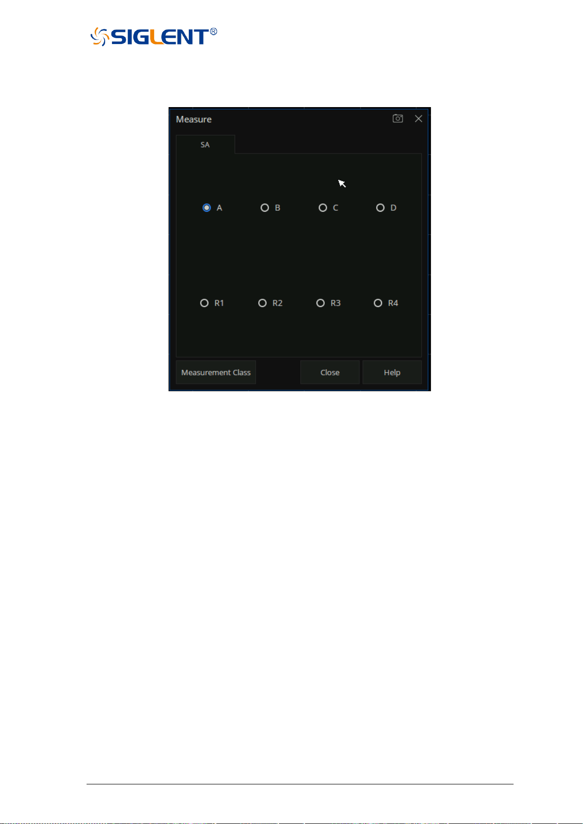
SNA5000A Vector Network Analyzer User Manual 138
After Spectrum Analysis measurement is displayed, press the Meas > SA > Other… to enter
the Measure dialog box and select the receiver used for measurement.
Figure 6-3 the interface of the Measure dialog box
6.3 Spectrum Analyzer Settings
6.3.1 Basic Setup
Press “Freq” on the front pane to enter the frequency setting menu , Set the frequency-related
parameters and functions of the analyzer. The sweep will restart every time the frequency
parameters are modified.
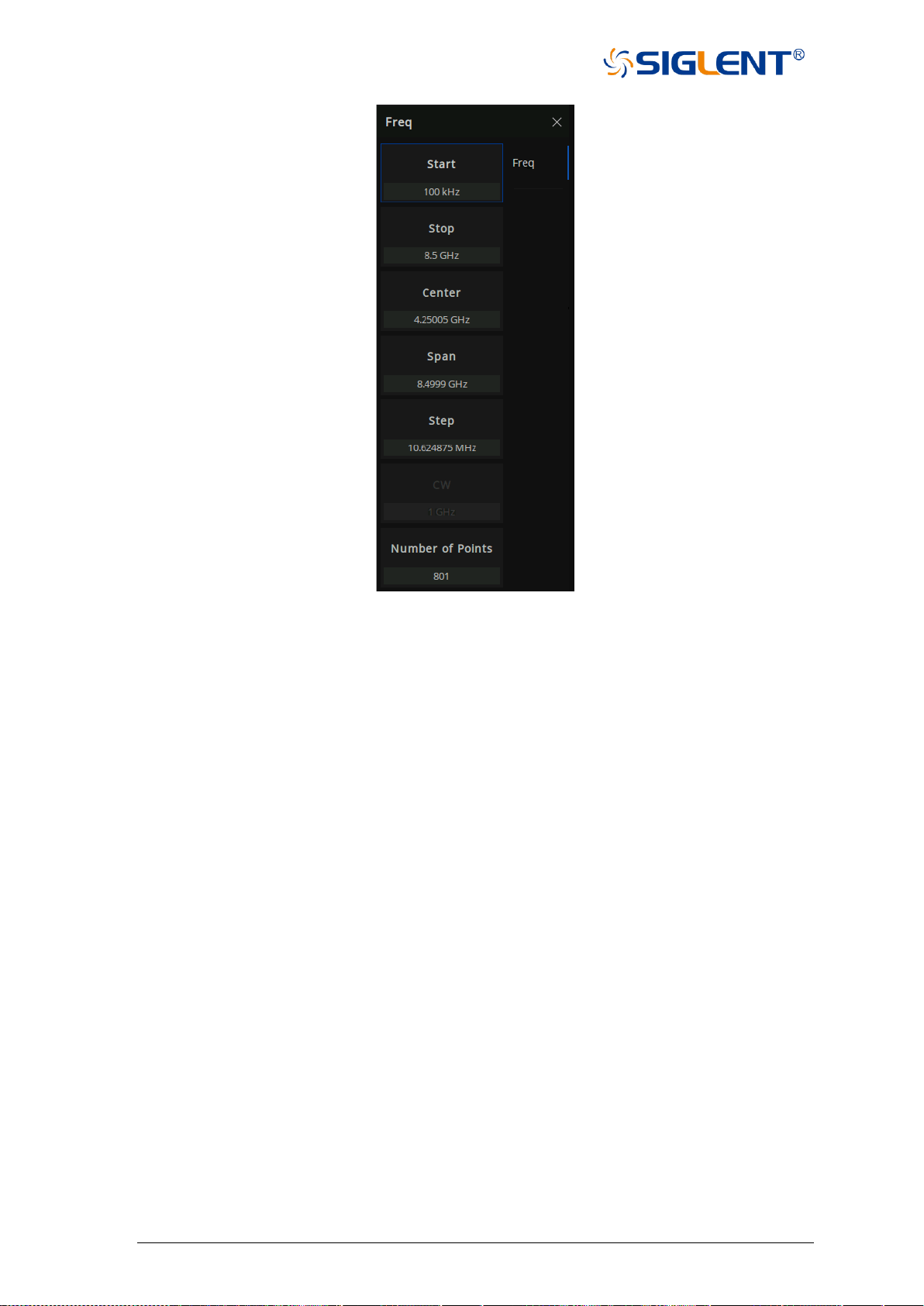
139 SNA5000A Vector Network Analyzer User Manual
Figure 6-4 frequency setting menu
The frequency range of a channel can be expressed by three parameters: Start Frequency,
Center Frequency and Stop Frequency. If any of the parameters change, the others will be
adjusted automatically in order to ensure the coupling relationship among them:
startstopspan
stopstartcenter
fff
)/2f(ff
−=
+=
, Where
span
f
is the span.
6.3.1.1 Start Frequency
Set the start frequency of the current sweep. The start and stop frequencies are displayed at
the bottom of the grid respectively.
● The span and center frequency vary with the start frequency when the Span does not
reach the minimum. For more details, please refer to “Span”.
● In Min Span, the start frequency, stop frequency and center frequency are the same value.
6.3.1.2 Stop Frequency
Set the stop frequency of the current sweep. The start and stop frequencies are displayed at
the lower right sides of the grid respectively.
● The span and center frequency vary with the stop frequency. The change of the span will
affect other system parameters. For more details, please refer to “Span”.
● In Zero Span, the start frequency, stop frequency and center frequency are always the

SNA5000A Vector Network Analyzer User Manual 140
same value.
6.3.1.3 Center Frequency
Set the center frequency of the current sweep. The center frequency and span values are
displayed at the bottom of the grid respectively.
● Modifying the center frequency will modify both the start frequency and stop frequency
when the span is constant (except when the start frequency or stop frequency reaches the
boundary).
● In Zero Span, the start frequency, stop frequency and center frequency are always the
same value.
6.3.1.4 Span
Set the span of the analyzer. Any change of this parameter will affect the frequency parameters
and restart the sweep.
Set the frequency range of the current sweep. Pay attention to the following points during use:
● The start and stop frequency vary with the span when the center frequency is constant.
● the span can be set down to 100 Hz and up to the maximum bandwidth.
● Modifying the span in non-zero span mode may cause an automatic change in both Freq
Step and RBW if they are in Auto mode. Besides, the change of RBW may influence VBW
(in Auto VBW mode).
● Variation in the span, RBW or VBW would cause a change in the sweep time.
6.3.1.5 Sweep Points
The number of points is the number of data items collected in one sweep.
The more scanning points, the more accurate the measurement results, but the longer the
scanning time. The less scanning points, the shorter the scanning time, can get the
measurement results faster.
6.3.1.6 Image Reject Type
The signal is mixed with the local oscillator to get an intermediate frequency signal, and the
mixer may produce a mirrored frequency signal. Therefore, it is necessary to change the local
oscillator or intermediate frequency to collect multiple groups of spectral data, and filter out the
image through the image suppression algorithm.
None: Selects 1 acquisitions, and mirror suppression is not performed.
Normal: Selects 4 acquisitions.
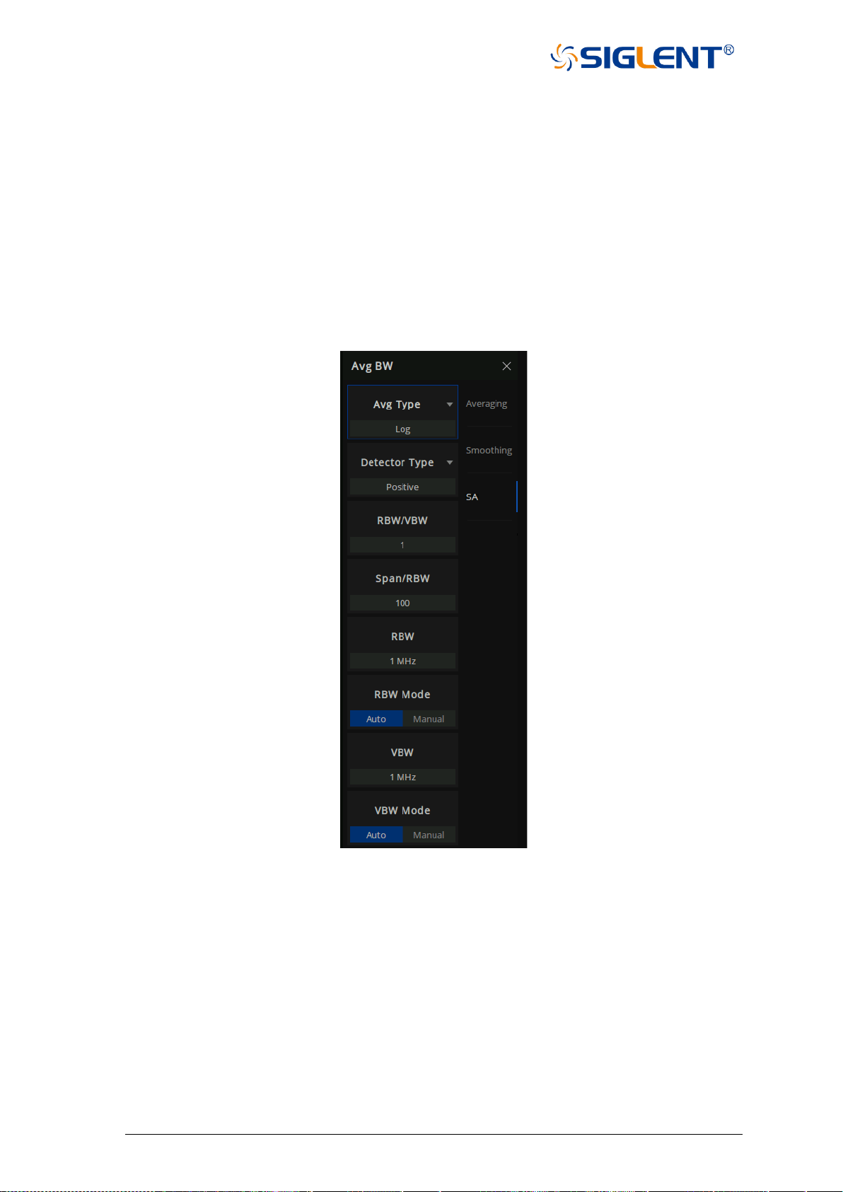
141 SNA5000A Vector Network Analyzer User Manual
Min: Selects 3 acquisitions.
Better: Selects 5 acquisitions.
Max: Selects 6 acquisitions.
Note: Only 3 sets of data can be acquisitions at most when the frequency point is below 40MHz.
6.3.2 Processing setup
Press the “AvgBw” on the front panel,prss AvgBW > SA to enter the menu interface of
processing setup menu.
Figure 6-5 the interface of processing setup menu
6.3.2.1 RBW
Set the RBW (resolution bandwidth) in order to distinguish between signals which have
frequency components that are near one another.
● Reducing the RBW will increase the frequency resolution. but lead to a longer sweep time
(influenced by both RBW and VBW when the sweep time is in automatic mode).
● RBW varies with the Span/RBW setting in Auto RBW mode.

SNA5000A Vector Network Analyzer User Manual 142
6.3.2.2 VBW
Set the video bandwidth in order to filter out the noise outside the video band.
● Reducing the VBW will smooth the trace and helps to highlight small signals from noise,
but it will also increase the sweep time (Sweep Time is affected by a combination of RBW
and VBW when it is in Auto mode).
● VBW varies with RBW when it is in Auto mode. While in Manual mode, VBW is not affected
by RBW.
6.3.2.3 RBW/VBW
Sets the ratio of Resolution Bandwidth to Video Bandwidth when the Video Bandwidth is in
Auto mode.
6.3.2.4 Span/RBW
Sets the ratio of Span to Resolution Bandwidth when the Resolution Bandwidth is in Auto mode.
6.3.2.5 Detector Type
The analyzer displays the sweep signal on the screen in the form of a trace. For each trace
point, the analyzer always captures all the data within a specific time interval and processes
(Peak, Average, etc.) the data using the detector currently selected, then it displays the
processed data (a single data point) on the screen.
Select an appropriate detector type according to the actual application in order to ensure the
accuracy of the measurement.
The available types are Positive Peak, Negative Peak, Sample and Average. The default is
Positive peak.
1. Positive Peak
For each trace point, Positive Peak detector displays the maximum value of data sampled
within the corresponding time interval.
2. Negative Peak
For each trace point, Negative Peak detector displays the minimum value of data sampled
within the corresponding time interval.
3. Sample
For each trace point, Sample detector displays the transient level corresponding to the
central time point of the corresponding time interval. This detector type is applicable to
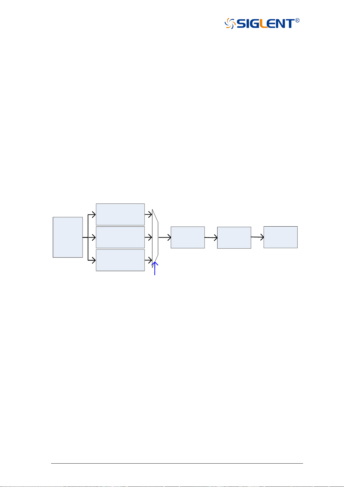
143 SNA5000A Vector Network Analyzer User Manual
noise or noise-like signal.
4. Normal
Normal detector (also called ROSENFELL Detector) displays the maximum value and the
minimum value of the sample data segment in turn: Odd-numbered data points display
the maximum value and even-numbered data points display the minimum value. In this
way, the amplitude variation range of the signal is clearly shown.
5. Average
For each trace point, Average detector displays the average value of data sampled within
the corresponding time interval.
6.3.2.6 Averaging Type
Average type refers to the processing mode of intermediate frequency data in data detection
and display detection, which affects the effect of trace average and detection average.
Power
(V^2)
RBW Voltage
LogPower
Detect
Avg Type
VBW
Trace
Figure 6-6 Flow chart of Average type
1. Log Power
Select the logarithmic (decibel) scale for all filtering and averaging processes. This scale
is "Video" because it is the most common display and analysis scale for the video signal
within analyzer. This scale is excellent for finding Sine/CW signals near noise.
2. Power Average
In this average type, all filtering and averaging processes work on the power (the square
of the magnitude) of the signal, instead of its log or envelope voltage. This scale is best
for real-time power measurement of complex signals.
3. Voltage Average
In this Average type, all filtering and averaging processes work on the voltage of the
envelope of the signal. This scale is suitable for observing rise and fall behavior of AM or
pulse-modulated signals such as radar and TDMA transmitters.
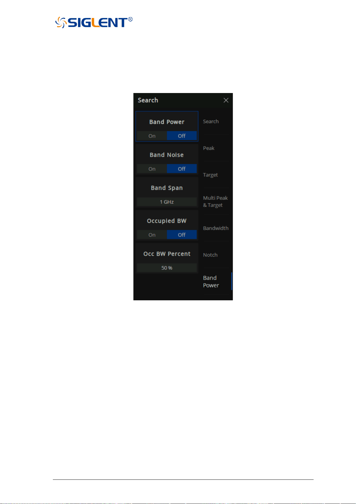
SNA5000A Vector Network Analyzer User Manual 144
6.4 Other features
Press “Search” on the front panel, click “Band Power” to enter the menu interface of
BandPower .
Figure 6-7 The menu interface of BandPower
6.4.1 Band Power
The total power of a specified frequency span.Before turning on the Band Power function the
marker point position and the frequency span should have be set.
The vertical dashed lines on either side of the marker indicate the span. The marked Y-axis
value is the measured power value, and the power value will be displayed in the upper right
corner.
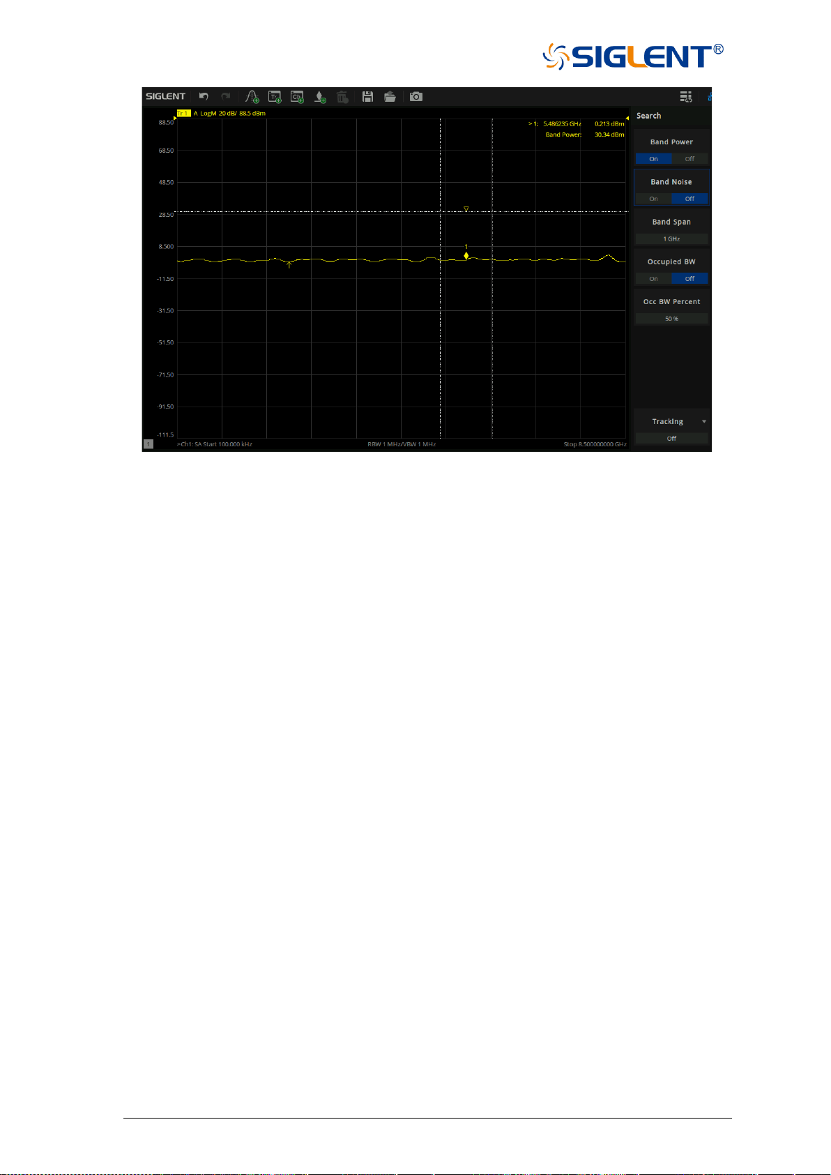
145 SNA5000A Vector Network Analyzer User Manual
Figure 6-8 Example of enabling Band Power
6.4.2 Band Noise
Specifies the normalization of the total power of a frequency span,(the power density). Before
turning on the Band Noise function the marker point position and the frequency span should
have be set.
The vertical dashed lines on either side of the marker indicate the span. The marked Y-axis
value is the measured power density value, and the power density value will be displayed in
the upper right corner.
The Band power and Band Noise functions can be enabled at the same time.
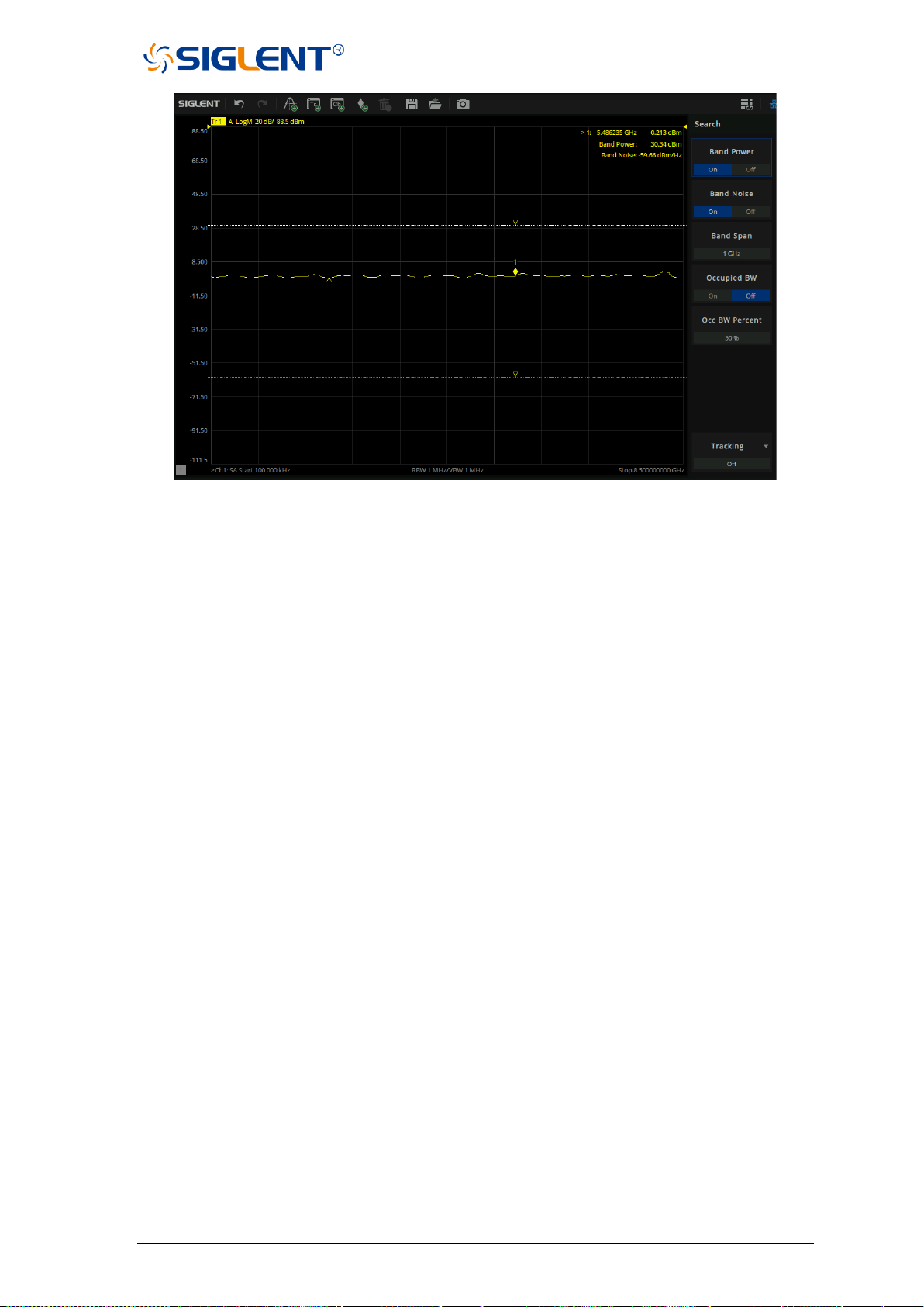
SNA5000A Vector Network Analyzer User Manual 146
Figure 6-9 Example of enabling Band Power and Band Noise
6.4.3 Occupied BW
Integrates the power within the whole span and calculates the bandwidth occupied by this
power according to the specified power ratio. Before turning on the Occupied BW function the
Occ BW Percent should have be set.
Vertical dashed lines on either side of the mark mark the span, indicating the percentage of
span. The Y-axis marked is the measured power value.The bandwidth and power of the span
will be displayed in the upper right corner.
BandPower and BandNoise are automatically turned off when Occupied BW is enabled.
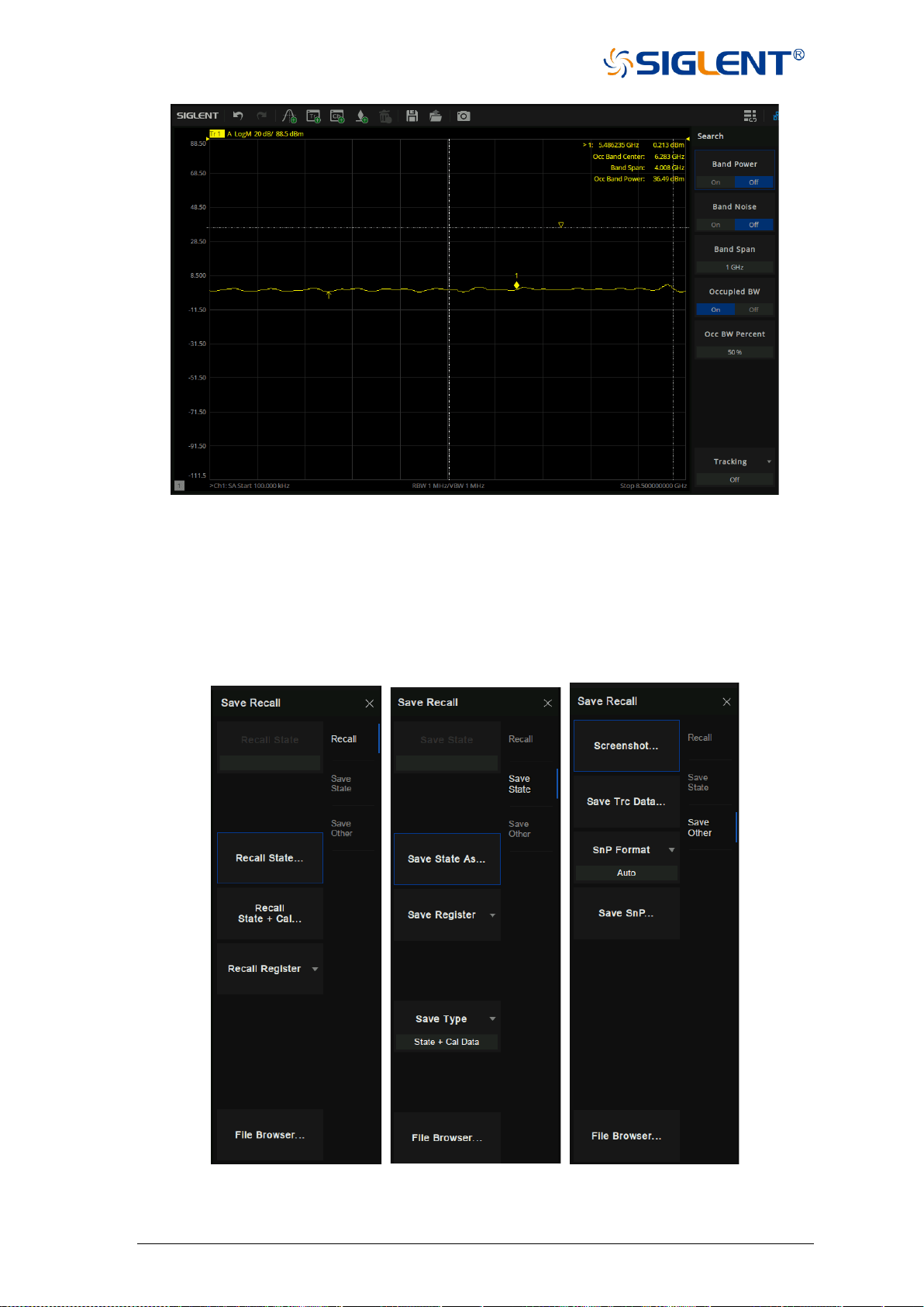
147 SNA5000A Vector Network Analyzer User Manual
Figure 6-10 Example of enabling Occuiped BW
7 Save and recall
The vector network analyzer supports save and recall functions for files of various formats.
Press the Save/Recall button on the front panel and select file, data, calibration data, and
images to save or recall. in the menu bar on the right side of the screen.
Figure 7-1 Operating interface

SNA5000A Vector Network Analyzer User Manual 148
Description of supported file formats:
⚫ STA file: The state file contains the configuration parameters (setup) of the
instrument.
⚫ CSA file: The calibration data and state file.
⚫ CSV file: Trace data.
⚫ SnP file: Also known as a Touchstone file. It contains the S parameter
information.
⚫ PNG/JPG/BMP file: Screenshot/exact copy of the display.
Save file:
⚫ Save the status of equipment:
Use the Save State As command in the Save State submenu to save the
equipment state.
⚫ Save the status and calibration data of equipment:
Select State+Cal Data command in the Save Type submenu to save the
equipment state and calibration data at the same time.
⚫ Save trace data:
Use the Save Trc Data command in the Save Other submenu to save the trace
data in CSV format; or use the Save SnP command to save the trace data in
SnP format. When saving the trace data in SnP format, you can select the
following formats: LinMag/Angle, LogMag/Angle and Real/Imaginary in the
SnP Format drop-down item.
⚫ Save screenshot:
Use the Screenshot command in the Save Other submenu to save the
screenshot. We can set the default path in the pop-up dialog box. The screenshot
file type can be saved as PNG/JPG/BMP file formats.
⚫ Save register data:
Use the Save Register command in the Save State submenu to save the data
in the register.
Recall file:
⚫ Recall status of equipment:
Use the Recall State command in the Recall submenu to select the required
equipment state in the .sta file format.
⚫ Recall the status and calibration data of equipment:
Use the Recall State + Cal command in the Recall submenu to select the
required equipment state and calibration data in .csa file format.
⚫ Recall register data:
Use the Recall Register command in Recall submenu to select the register data
to be recalled.
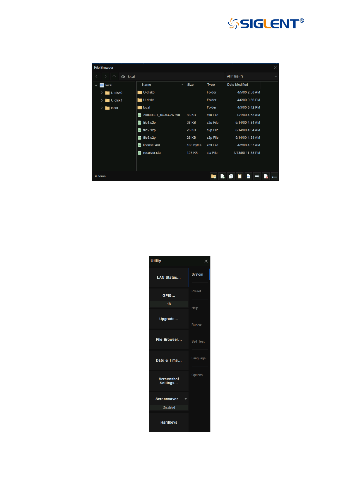
149 SNA5000A Vector Network Analyzer User Manual
File management:
Click File Browser command to open the file browser, File management can be carried
out in the file browser.
Figure 7-2 File management interface
8 System setting
Press the System button on the front panel. We can set the IP address, set the date,
restore the factory settings, consult the help document, set the buzzer, self-detection, language
setting, obtain the software and hardware information of the device, and license management
in the menu on the right side of the screen.
Figure 8-1 System setting interface
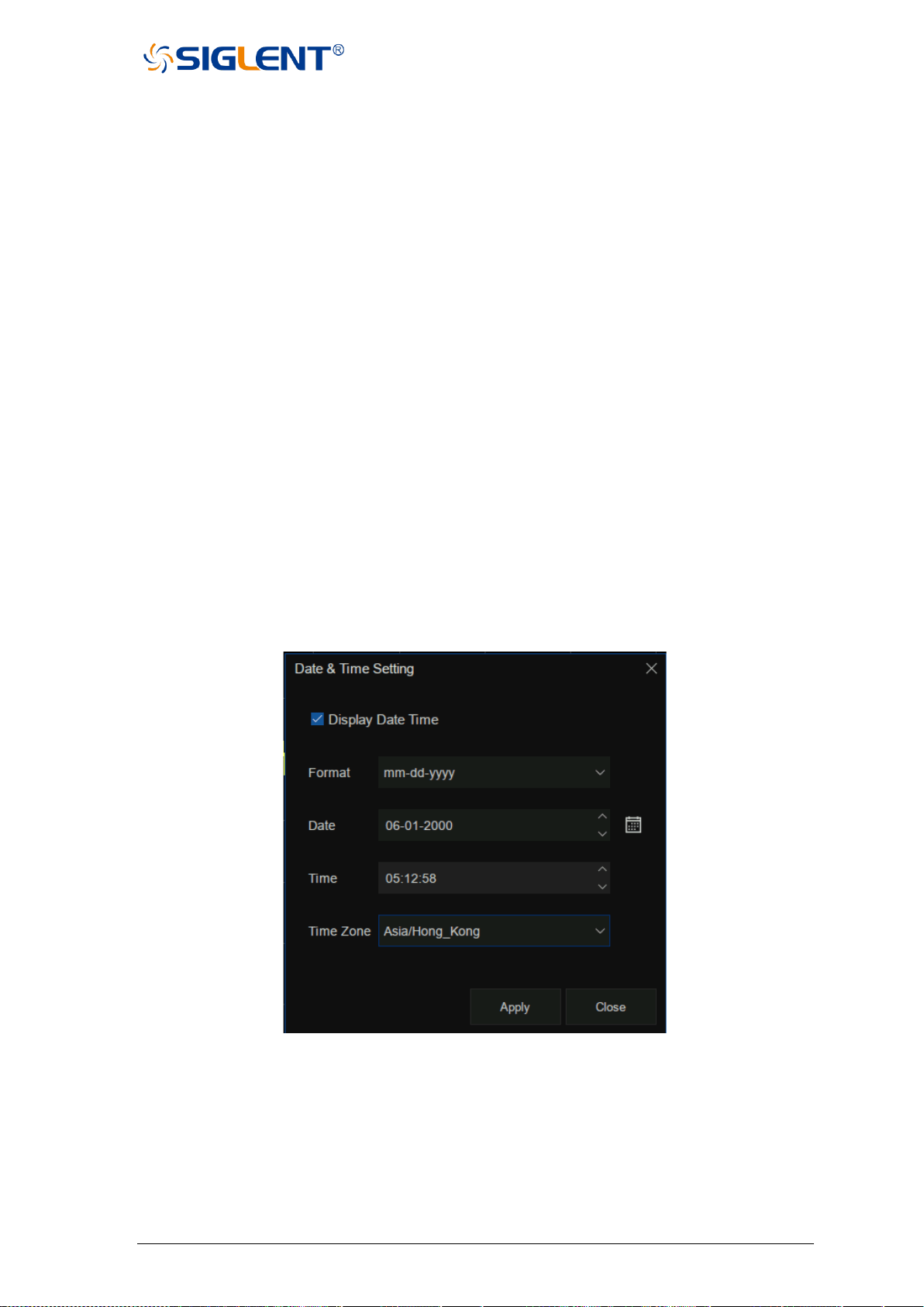
SNA5000A Vector Network Analyzer User Manual 150
Communication interface setting:
• LAN setting:
We can select static or dynamic allocation of LAN-related parameters. Use LAN
Status command in System submenu to set LAN parameters.
• Set GPIB port number:
Use the GPIB command in the System submenu to set the GPIB port number.
Firmware upgrade:
Store the.ADS file in the firmware upgrade package downloaded from the official website
in the U disk root directory, insert the U disk into the USB port of the vector network analyzer,
click the Upgrade command in the System submenu, select the required file in the pop-up
file browser, and click OK to upgrade the firmware. The firmware upgrade process may last
for several minutes. When the upgrade is completed, the device will automatically restart.
Any operation that interrupts the upgrade process may cause the upgrade to fail or even the
device cannot start normally. Please keep the U disk stable and the power supply of the
equipment normal during the firmware upgrade process.
Date/Time setting:
Use the Date & Time command in the System submenu to set the date/time. You can set
whether to display the date/time and display the format at the bottom right of the screen and
modify the date/time value.
Figure 8-2 Date/Time setting interface
Screenshot setting:
Use the Screenshot Settings command in the System submenu to set the screen
capture parameters.
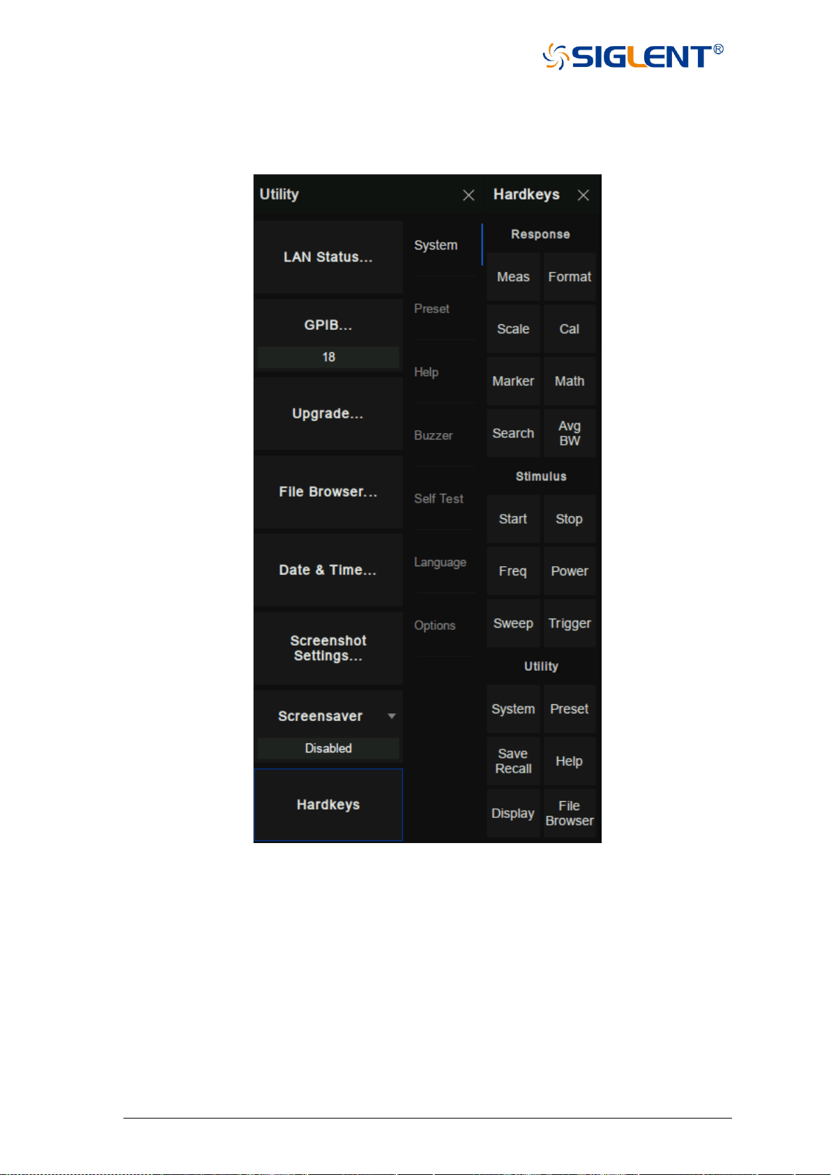
151 SNA5000A Vector Network Analyzer User Manual
Hardkeys:
The Hardkeys command in the System submenu can be used to open the function of
hardkeys on the right side of the screen so that the vector network analyzer can be operated
without operating the function keys on the front panel.
Figure 8-3 Hardkeys
Preset:
Preset operation and related settings can be performed in Preset submenu.
• Preset:
Use the Preset command to reset immediately according to the setting reset
options.
• Preset Option:
Use the Preset Option command to set the reset options, and to determine the
preset source:
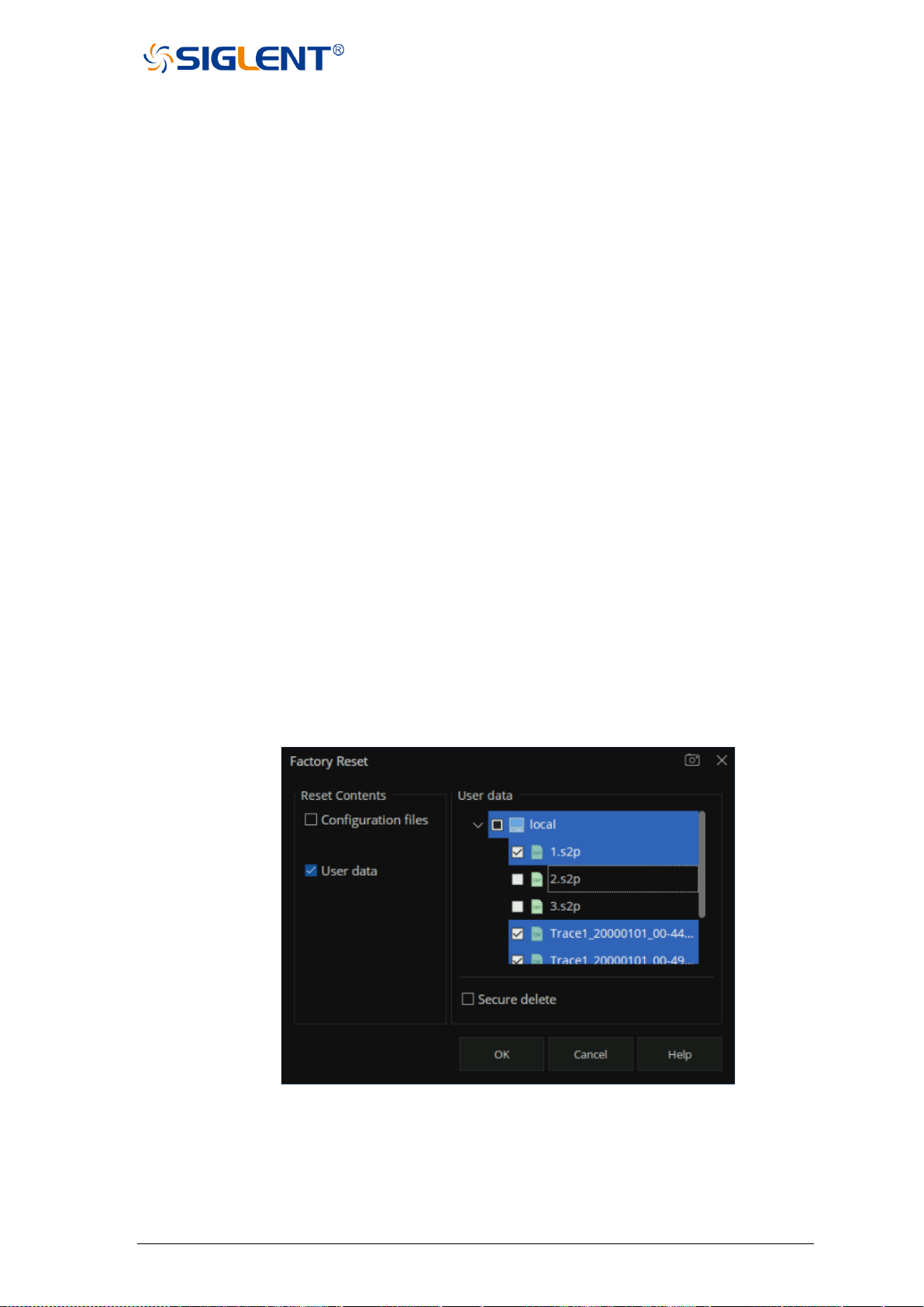
SNA5000A Vector Network Analyzer User Manual 152
1. Default: Load default parameters.
2. Last: When the equipment is shut down, the current state will be saved
automatically. Use this option to restore to the last shutdown state.
3. User: Restore the equipment to the user-specified state.
• User Preset:
Use the User Preset command to specify the user preset status information file.
• Confirm Preset:
Use the Confirm Preset command to set whether to confirm before reset.
• Power On Option:
Use the Power On Option command to set the default source of equipment reset
when the equipment starts.
• Power On-Line:
Use the Power On-Line command to set whether the device starts automatically
when it is powered on.
• Factory Reset:
Configuration files(Selected by default)
Indicates that the equipment is restored to the factory default state, but the files saved
by the user to local will not be deleted.
User data
(Optional), user can selectively delete the files saved to local.
Figure 8-4 Select the saved file
Configuration files and User data
If user select both, the equipment is restored to the factory default state and deletes
the files saved to local by users.

153 SNA5000A Vector Network Analyzer User Manual
Help information:
In the Help submenu, we can open the help document (Help command) or view the
equipment information (About command).
Buzzer:
We can set the sound in the Buzzer submenu.
• Buzzer: Use the Buzzer command to turn the device sound on or off.
• Complete Test: Use the Complete Test command to test the completion tone.
• Complete Buzzer: Use the Complete Buzzer command to turn the
completion tone on or off.Warning Test: Use the Warning Test
command to test the alarm tone.
• Warning Buzzer: Use the Warning Buzzer command to turn on or off the alarm tone.
• Touch Buzzer: Use the Touch Buzzer command to turn on or off the touchscreen
keystone.

SNA5000A Vector Network Analyzer User Manual 154
Self-Test:
In the Self Test submenu, we can perform keyboard self-test (Key Test command), touch
screen self-test (Touch Test command), screen self-test (Screen Test command) and LED
self test (LED Test command).
System language:
The Language command in the Language submenu can be used to change the language
of the equipment. Simplified Chinese and English are supported.
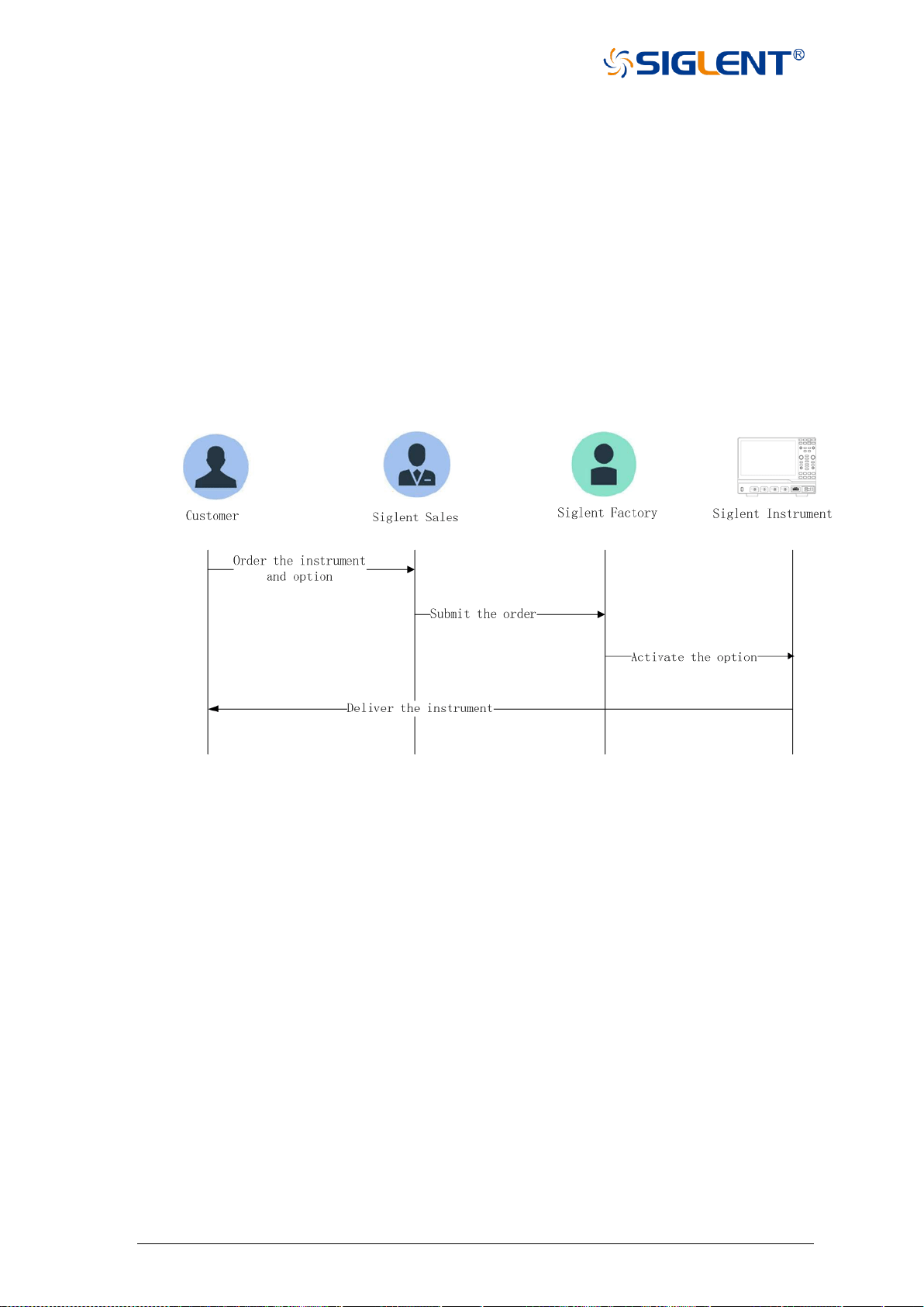
155 SNA5000A Vector Network Analyzer User Manual
9 Service and support
9.1 Ordering and activating the options
There are two ways for you:
1. Pre-activate the options by Siglent factory.
If you order a instrument and options, Siglent factory will activate the options for you before
delivery.
2. Post-activate the options by yourself.
If you want to activate options on a instrument that you are using.
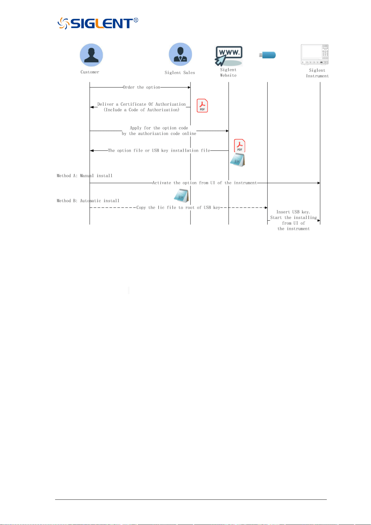
SNA5000A Vector Network Analyzer User Manual 156
9.2 Warranty overview
SIGLENT guarantees that the products produced and sold will not have defects in
materials and technology within three years from the date of delivery by authorized distributors.
If the product is defective within the warranty period, SIGLENT will provide repair or
replacement service according to the detailed provisions of the warranty.
For service or a complete copy of the warranty, please contact your nearest SIGLENT
sales and service office. SIGLENT makes no other warranty, express or implied, except as
provided in this summary or the applicable warranty, including but not limited to the implied
warranty of merchantability and special applicability. SIGLENT shall not be liable for any
indirect, special or consequential damages.

157 SNA5000A Vector Network Analyzer User Manual
Tel: +49(0)-821-666 0 111 0
Fax: +49(0)-821-666 0 111 22
Email: info-eu@siglent.com
Website: www.siglenteu.com
About SIGLENT
SIGLENT is an international high-tech company, concentrating on R&D, sales,
production and services of electronic test & measurement instruments.
SIGLENT first began developing digital oscilloscopes independently in 2002.
After more than a decade of continuous development, SIGLENT has extended
its product line to include digital oscilloscopes, isolated handheld
oscilloscopes, function/arbitrary waveform generators, RF/MW signal
generators, spectrum analyzers, vector network analyzers, digital multimeters,
DC power supplies, electronic loads and other general purpose test
instrumentation. Since its first oscilloscope was launched in 2005, SIGLENT
has become the fastest growing manufacturer of digital oscilloscopes. We
firmly believe that today SIGLENT is the best value in electronic test &
measurement.
Headquarters:
SIGLENT Technologies Co., Ltd
Add: Bldg No.4 & No.5, Antongda Industrial
Zone, 3rd Liuxian Road, Bao'an District,
Shenzhen, 518101, China
Tel: + 86 755 3688 7876
Fax: + 86 755 3359 1582
Email: sales@siglent.com
Website: int.siglent.com
North America:
SIGLENT Technologies America, Inc
6557 Cochran Rd Solon, Ohio 44139
Tel: 440-398-5800
Toll Free: 877-515-5551
Fax: 440-399-1211
Email: info@siglent.com
Website: www.siglentna.com
Europe:
SIGLENT Technologies Germany GmbH
Add: Staetzlinger Str. 70
86165 Augsburg, Germany
Tel: +49(0)-821-666 0 111 0
Fax: +49(0)-821-666 0 111 22
Email: info-eu@siglent.com
Website: www.siglenteu.com
Follow us on
Facebook: SiglentTech