Version Info
Version
Date
Remarks
V1.0
2023.02

Preface
Preface
Dear customers,
Congratulations! Thank you for buying Micsig instrument. Please read this manual carefully before use and
particularly pay attention to the “Safety Precautions”.
If you have read this manual, please keep it properly for future reference.
The information contained herein are furnished in an “as-is” state, and may be subject to change in future versions
without notice.
The standard applicable for this product: GB/T15289-2013.

Table of Contents
i
Table of Contents
TABLE OF CONTENTS ........................................................................................................................................................................... I
CHAPTER 1. SAFETY PRECAUTIONS .............................................................................................................................................. 1
1.1 SAFETY PRECAUTIONS ............................................................................................................................................................................................. 1
1.2 SAFETY TERMS AND SYMBOLS ............................................................................................................................................................................... 5
CHAPTER 2. QUICK START GUIDE OF OSCILLOSCOPE ............................................................................................................. 8
2.1 INSPECT PACKAGE CONTENTS ................................................................................................................................................................................ 9
2.2 USE THE BRACKET ................................................................................................................................................................................................ 10
2.3 SIDE PANEL ........................................................................................................................................................................................................... 11
2.4 REAR PANEL .......................................................................................................................................................................................................... 12
2.5 TOP PANEL ............................................................................................................................................................................................................ 13
2.6 FRONT PANEL........................................................................................................................................................................................................ 14

ii
2.7 POWER ON/OFF THE OSCILLOSCOPE .................................................................................................................................................................. 15
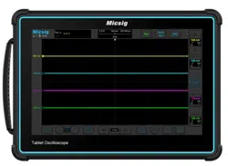
2.8 UNDERSTAND THE OSCILLOSCOPE DISPLAY INTERFACE .................................................................................................................................. 16
2.9 INTRODUCTION BASIC OPERATIONS OF TOUCH SCREEN ................................................................................................................................. 22
2.10 MOUSE OPERATION ........................................................................................................................................................................................... 24
2.11 CONNECT PROBE TO THE OSCILLOSCOPE ........................................................................................................................................................ 25
2.12 USE AUTO ............................................................................................................................................................................................................ 26
2.13 LOAD FACTORY SETTINGS ................................................................................................................................................................................. 31
2.14 USE AUTO-CALIBRATION ................................................................................................................................................................................... 31
2.15 PASSIVE PROBE COMPENSATION ...................................................................................................................................................................... 33
2.16 MODIFY THE LANGUAGE .................................................................................................................................................................................... 38
CHAPTER 3 AUTOMOTIVE TEST ................................................................................................................................................... 39
3.1 CHARGING/START CIRCUIT ................................................................................................................................................................................. 39
3.1.1
12V Charging ................................................................................................................................................................................................ 41
3.1.2
24V Charging ................................................................................................................................................................................................ 43

Table of Contents
iii
3.1.3
Alternator AC Ripple .................................................................................................................................................................................. 44
3.1.4
Ford Focus Smart Generator .................................................................................................................................................................... 46
3.1.5
12V Start ............................................................................................................................................................................................................ 48
3.1.6
24V Start ......................................................................................................................................................................................................... 50
3.1.7
Cranking Current ........................................................................................................................................................................................ 51
3.2 SENSOR TESTS ....................................................................................................................................................................................................... 53
3.2.1
ABS ....................................................................................................................................................................................................................... 54
3.2.2
Accelerator pedal ........................................................................................................................................................................................... 55
3.2.3
Air Flow Meter ................................................................................................................................................................................................ 58
3.2.4
Camshaft ............................................................................................................................................................................................................ 61
3.2.5
Coolant Temperature ................................................................................................................................................................................... 63
3.2.6
Crankshaft ......................................................................................................................................................................................................... 65
3.2.7 Distributor ............................................................................................................................................................................................................ 68
3.2.8
Fuel pressure .................................................................................................................................................................................................... 70

iv
3.2.9
Knock ................................................................................................................................................................................................................... 72
3.2.10
Lambda ............................................................................................................................................................................................................ 74
3.2.11
MAP ................................................................................................................................................................................................................... 78
3.2.12
Road Speed ..................................................................................................................................................................................................... 80
3.2.13
Throttle Position.......................................................................................................................................................................................... 82
3.3 ACTUATORS ............................................................................................................................................................................................................ 85
3.3.1
Carbon canister solenoid valve ................................................................................................................................................................ 85
3.3.2
Disel Glow Plugs ............................................................................................................................................................................................. 88
3.3.3
EGR Solenoid Valve ....................................................................................................................................................................................... 90
3.3.4
Fuel Pump ......................................................................................................................................................................................................... 92
3.3.5
Idle speed control valve ............................................................................................................................................................................ 94
3.3.6
Injector (gasoline engine) ....................................................................................................................................................................... 96
3.3.7
Injector (Diesel) .............................................................................................................................................................................................. 98
3.3.8
Pressure regulator ................................................................................................................................................................................... 100
3.3.9
Quantity (Flow) control valve ............................................................................................................................................................... 102

Table of Contents
v
3.3.10
Throttle Servo Motor .............................................................................................................................................................................. 104
3.3.11
Variable speed cooling fan ................................................................................................................................................................... 106
3.3.12
Variable valve timing ............................................................................................................................................................................. 109
3.4 IGNITION TESTS .................................................................................................................................................................................................. 111
3.4.1
Primary ........................................................................................................................................................................................................... 112
3.4.2
Secondary ....................................................................................................................................................................................................... 115
3.4.3
Primary + Secondary ................................................................................................................................................................................ 117
3.5 NETWORKS .......................................................................................................................................................................................................... 120
3.5.1
CAN High & CAN Low ................................................................................................................................................................................ 120
3.5.2
LIN Bus ............................................................................................................................................................................................................ 122
3.5.3
FlexRay Bus ................................................................................................................................................................................................... 125
3.5.4
K line ................................................................................................................................................................................................................. 127
3.6 COMBINATION TESTS.......................................................................................................................................................................................... 129
3.6.1
Crankshaft + Camshaft ............................................................................................................................................................................. 129

vi
3.6.2
Crankshaft + Primary ignition .............................................................................................................................................................. 131
3.6.3
Primary ignition + Injector voltage.................................................................................................................................................... 133
3.6.4
Crankshaft + Camshaft + Injector + Secondary Ignition .......................................................................................................... 135
CHAPTER 4 HORIZONTAL SYSTEM ............................................................................................................................................ 137
4.1 MOVE THE WAVEFORM HORIZONTALLY....................................................................................................................................................... 139
4.2 ADJUST THE HORIZONTAL TIME BASE (TIME/DIV) .................................................................................................................................... 140
4.3 PAN AND ZOOM SINGLE OR STOPPED ACQUISITIONS ................................................................................................................................. 142
4.4 ROLL, XY .......................................................................................................................................................................................................... 143
4.5 ZOOM MODE .................................................................................................................................................................................................... 152
CHAPTER 5 VERTICAL SYSTEM .................................................................................................................................................. 155
5.1 OPEN/CLOSE WAVEFORM (CHANNEL, MATH, REFERENCE WAVEFORMS)................................................................................................ 157
5.2 ADJUST VERTICAL SENSITIVITY ........................................................................................................................................................................ 162
5.3 ADJUST VERTICAL POSITION ............................................................................................................................................................................. 163
5.4 OPEN CHANNEL MENU ...................................................................................................................................................................................... 163

Table of Contents
vii
5.4.1 Set Channel Coupling .................................................................................................................................................................................... 165
5.4.2 Set Bandwidth Limit...................................................................................................................................................................................... 167
5.4.3 Waveform Inversion ...................................................................................................................................................................................... 168
5.4.4 Set Probe Type ................................................................................................................................................................................................. 169
5.4.5 Set Probe Attenuation Coefficient ........................................................................................................................................................... 170
5.4.6 Labels ................................................................................................................................................................................................................... 171
CHAPTER 6 TRIGGER SYSTEM .................................................................................................................................................... 173
6.1 TRIGGER AND TRIGGER ADJUSTMENT .............................................................................................................................................................. 174
6.2 EDGE TRIGGER .................................................................................................................................................................................................... 187
6.3 PULSE WIDTH TRIGGER ..................................................................................................................................................................................... 191
6.4 LOGIC TRIGGER ................................................................................................................................................................................................... 199
6.5 NTH EDGE TRIGGER ........................................................................................................................................................................................... 205
6.6 RUNT TRIGGER .................................................................................................................................................................................................... 208
6.7 SLOPE TRIGGER ................................................................................................................................................................................................... 210

viii
6.8 TIMEOUT TRIGGER ............................................................................................................................................................................................. 215
6.9 VIDEO TRIGGER ................................................................................................................................................................................................... 218
6.10 SERIAL BUS TRIGGER....................................................................................................................................................................................... 223
CHAPTER 7 ANALYSIS SYSTEM ................................................................................................................................................... 224
7.1 AUTOMATIC MEASUREMENT ............................................................................................................................................................................. 225
7.2 FREQUENCY METER MEASUREMENT ............................................................................................................................................................... 238
7.3 CURSOR ................................................................................................................................................................................................................ 239
7.4 PHASE RULERS .................................................................................................................................................................................................... 244
CHAPTER 8 SCREEN CAPTURE, MEMORY DEPTH AND WAVEFORM STORAGE .......................................................... 246
8.1 SCREEN CAPTURE FUNCTION ............................................................................................................................................................................ 247
8.2 VIDEO RECORDING ............................................................................................................................................................................................. 250
8.3 WAVEFORM STORAGE ........................................................................................................................................................................................ 251
8.4 OSCILLOSCOPE SETTING SAVE ............................................................................................................................................................................ 258
CHAPTER 9 MATH AND REFERENCE ........................................................................................................................................ 260

Table of Contents
ix
9.1 DUAL WAVEFORM CALCULATION ..................................................................................................................................................................... 261
9.2 FFT MEASUREMENT .......................................................................................................................................................................................... 266
9.3 ADVANCED MATH ............................................................................................................................................................................................... 273
9.4 REFERENCE WAVEFORM CALL .......................................................................................................................................................................... 277
CHAPTER 10 DISPLAY SETTINGS............................................................................................................................................... 281
10.1 WAVEFORM SETTINGS ..................................................................................................................................................................................... 283
10.2 GRATICULE SETTING ........................................................................................................................................................................................ 283
10.3 PERSISTENCE SETTING .................................................................................................................................................................................... 284
10.4 HORIZONTAL EXPANSION CENTER ................................................................................................................................................................. 287
10.5 COLOR TEMPERATURE SETTING .................................................................................................................................................................... 287
10.6 TIME BASE MODE SELECTION ........................................................................................................................................................................ 288
CHAPTER 11 SAMPLING SYSTEM .............................................................................................................................................. 289
11.1 SAMPLING OVERVIEW ...................................................................................................................................................................................... 290
11.2 RUN/STOP KEY AND SINGLE SEQ KEY ........................................................................................................................................................ 296

x
11.3 SELECT SAMPLING MODE ............................................................................................................................................................................... 297
11.4 RECORD LENGTH AND SAMPLING RATE ........................................................................................................................................................ 303
CHAPTER 12 SERIAL BUS TRIGGER AND DECODE (OPTIONAL) ..................................................................................... 307
12.1 UART (RS232/RS422/RS485) BUS TRIGGER AND DECODE .............................................................................................................. 312
12.2 LIN BUS TRIGGER AND DECODE .................................................................................................................................................................... 324
12.3 CAN BUS TRIGGER AND DECODE .................................................................................................................................................................. 332
12.4 SPI BUS TRIGGER AND DECODE .................................................................................................................................................................... 339
12.5 I2C BUS TRIGGER AND DECODE .................................................................................................................................................................... 346
12.6 ARINC429 BUS TRIGGER AND DECODE...................................................................................................................................................... 354
12.7 1553B BUS TRIGGER AND DECODE.............................................................................................................................................................. 362
CHAPTER 13 HOMEPAGE FUNCTIONS ..................................................................................................................................... 370
13.1 OSCILLOSCOPE (SEE CHAPTERS 2~12) ....................................................................................................................................................... 372
13.2 APP STORE ........................................................................................................................................................................................................ 372
13.3 SETTINGS ........................................................................................................................................................................................................... 376

Table of Contents
xi
13.4 FILE MANAGER ................................................................................................................................................................................................. 383
13.5 CALCULATOR ..................................................................................................................................................................................................... 384
13.6 BROWSER .......................................................................................................................................................................................................... 384
13.7 GALLERY ............................................................................................................................................................................................................ 385
13.8 CALENDAR ......................................................................................................................................................................................................... 388
13.9 ELECTRONIC TOOLS ......................................................................................................................................................................................... 388
13.10 CLOCK ............................................................................................................................................................................................................. 389
13.11 POWER OFF .................................................................................................................................................................................................... 392
CHAPTER 14 REMOTE CONTROL ............................................................................................................................................... 395
14.1 HOST COMPUTER ............................................................................................................................................................................................. 396
14.1.1 Installation of Host Computer Software ............................................................................................................................................ 396
14.1.2 Connection of Host Computer................................................................................................................................................................. 397
14.1.3 Main Interface Introduction ................................................................................................................................................................... 399
14.1.4 Operation Interface Introduction ......................................................................................................................................................... 401

xii
14.1.5 Storage and View of Pictures and Videos .......................................................................................................................................... 402
14.2 MOBILE REMOTE CONTROL ............................................................................................................................................................................ 404
CHAPTER 15 UPDATE AND UPGRADE FUNCTIONS.............................................................................................................. 408
15.1 SOFTWARE UPDATE ......................................................................................................................................................................................... 409
15.2 ADD OPTIONAL FUNCTIONS ............................................................................................................................................................................ 410
CHAPTER 16 REFERENCE ............................................................................................................................................................. 413
16.1 MEASUREMENT CATEGORY ............................................................................................................................................................................. 414
16.2 POLLUTION DEGREE ........................................................................................................................................................................................ 415
CHAPTER 17 TROUBLESHOOTING ............................................................................................................................................ 417
CHAPTER 18 SERVICES AND SUPPORT .................................................................................................................................... 423
ANNEX ................................................................................................................................................................................................ 425
ANNEX A:MAINTENANCE AND CARE OF OSCILLOSCOPE ....................................................................................................................................... 425
ANNEX B: ACCESSORIES ............................................................................................................................................................................................ 428

Chapter 1. Safety Precautions
1
Chapter 1. Safety Precautions
1.1 Safety Precautions
The following safety precautions must be understood to avoid personal injury and prevent damage to this product or
any products connected to it. To avoid possible safety hazards, it is essential to follow these precautions while using
this product.
Only professionally trained personnel can operate the maintenance procedure.
Avoid fire and personal injury.
Use proper power cord. Use only the power cord specified for this product and certified for the country/region
of use.
Connect and disconnect probes properly. Connect the instrument probe correctly, and its ground terminal is
ground phase. Do not connect or disconnect probes or test leads while they are connected to a voltage source.

2
Disconnect the probe input and the probe reference lead from the circuit under test before disconnecting the
probe from the measurement product.
Ground the product. To avoid electric shock, the instrument grounding conductor must be connected to
earth ground.
Observe all terminal ratings. To avoid fire or shock hazard, observe all rating and markings on the product.
Consult the product manual for further information of ratings before making connections to the product.
User correct probes. To avoid excessive electric shock, use only correct rated probes for any measurement.
Disconnect AC power. The adapter can be disconnected from AC power and the user must be able to access the
adapter at any time.
Do not operate without covers. Do not operate the product with covers or panels removed.
Do not operate with suspected failures. If you suspect that there is damage to this product, have it inspected
by service personnel designated by Micsig.

Chapter 1. Safety Precautions
3
Use adapter correctly. Supply power or charge the equipment by power adapter designated by Micsig, and
charge the battery according to the recommended charging cycle.
Avoid exposed circuitry. Do not touch exposed connections and components when power is present.
Provide proper ventilation.
Do not operate in wet/damp conditions.
Do not operate in a flammable and explosive atmosphere.
Keep product surfaces clean and dry.
The disturbance test of all models complies with Class A standards, based on EN61326:1997+A1+A2+A3,
but do not meet Class B standards.
Measurement Category
The ATO series oscilloscope is intended to be used for measurements in Measurement Category I.

4
Measurement Category Definition
Measurement category I is for measurements performed on circuits not directly connected to the MAINS. Examples
are measurements on circuits not derived from MAINS, and specially protected (internal) MAINS derived circuits.
In the latter case, transient stresses are variable; for that reason, the user must understand the transient withstand
capability of the equipment.
Warning
IEC Measurement Category. Under IEC Category I mounting conditions, the input terminal can be connected to the
circuit terminal with a maximum line voltage of 300Vrms. To avoid the risk of electric shock, the input terminal
should not be connected to the circuit with a line voltage greater than 300Vrms. Instantaneous overvoltage is
present in circuits that are isolated from the mains supply. The ATO series digital oscilloscope is designed to safely
withstand sporadic transient overvoltage up to 1000Vpk. Do not use this equipment for any measurements in
circuits where the instantaneous overvoltage exceeds this value.

Chapter 1. Safety Precautions
5
1.2 Safety Terms and Symbols
Terms in the manual
These terms may appear in this manual:
Warning. Warning statements indicate conditions or practices that could result in injury or loss of life.
Caution. Caution statements indicate conditions or practices that could result in damage to this product or
other property.
Terms on the product
These terms may appear on the product:
Danger indicates an injury hazard immediately accessible as you read the marking.
Warning indicates an injury hazard not immediately accessible as you read the marking.
Caution indicates a hazard to this product or other properties.
6
Symbols on the product
The following symbols may appear on the product:
Hazardous Voltage Caution Refer to Manual Protective Ground Terminal
Chassis Ground Measurement Ground Terminal
Please read the following safety precautions to avoid personal injury and prevent damage to this product or
any products connected to it. To avoid possible hazards, this product can only be used within the specified
scope.
Warning
If the instrument input port is connected to a circuit with the peak voltage higher than 42V or the power exceeding
4800VA, to avoid electric shock or fire:

Chapter 1. Safety Precautions
7
User only insulated voltage probes supplied with the instrument, or the equivalent product indicated in the
schedule.
Before use, inspect voltage probes, test leads, and accessories for mechanical damage and replace when
damaged.
Remove voltage probes and accessories not in use.
Plug the battery charger into the AC outlet before connecting it to the instrument.

8
Chapter 2. Quick Start Guide of Oscilloscope
This chapter contains checks and operations of the oscilloscope. You are recommended to read them carefully to
understand appearance, power on/off, settings and related calibration requirements of the ATO series oscilloscope.
Inspect package contents
Mouse operation
Use bracket
Connect probe to the oscilloscope
Side panel & rear panel
Use automatic
Front panel
Use factory settings
Power on/off the oscilloscope
Use auto-calibration
Understand the oscilloscope display interface
Passive probe compensation
Introduction to basic operations of oscilloscope
Modify the language

Chapter 2. Quick Start Guide of Oscilloscope
9
2.1 Inspect Package Contents
When you open package after receipt, please check the instrument according to the following steps.
1) Inspect if there is any damage caused by transportation
If the package or foam is found to be severely damaged, please retain it until the instrument and accessories
pass the electrical and mechanical properties test.
2) Inspect the accessories
A detailed description is given in “
Annex B” of this manual. You can refer it to check if the accessories are
complete. If the accessories are missing or damaged, please contact Micsig’s agent or local office.
3) Inspect the instrument
If any damage to oscilloscope is found by the appearance inspection or it fails to pass the performance test,
please contact Micsig’s agent or local office. If the instrument is damaged due to transportation, please retain
the package and contact the transportation company or Micsig’s agent, and Micsig will make arrangement.
10
2.2 Use the Bracket
Put the front panel of the oscilloscope flatly on the table. Use your two index fingers to hold the underside of the
bracket and open the bracket by slightly upwards force, as shown in Figure 2-1.
Figure 2-1 Open Bracket
Chapter 2. Quick Start Guide of Oscilloscope
11
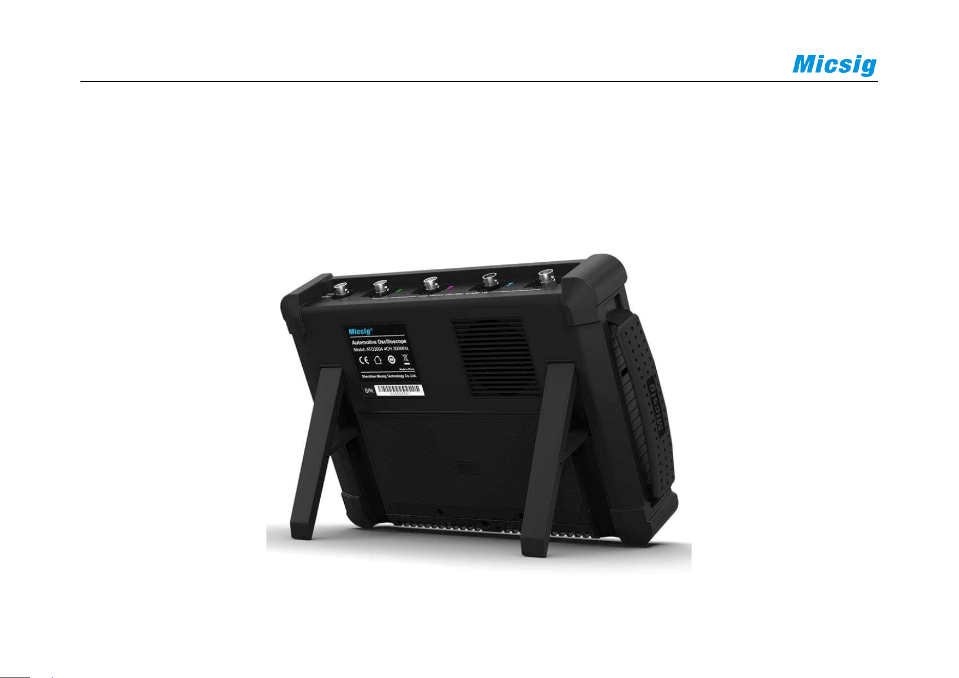
2.3 Side Panel
Figure 2-2 Side Panel
There are various interfaces on the side of the oscilloscope, from left to right: Power-on button, Grounding, Probe
compensation signal output, USB Host, HDMI, USB Device, Power-off lock, and Power port.
12
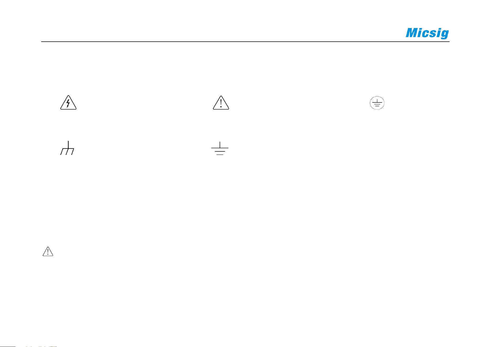
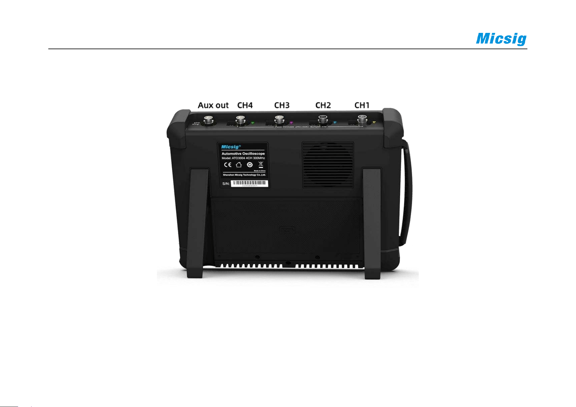
2.4 Rear Panel
Figure 2-3 Rear Panel
a) Ch1 – Ch4 are signal measurement channels
Chapter 2. Quick Start Guide of Oscilloscope
13
b) Aux out is an auxiliary channel, which is mainly used to measure the waveform refresh rate of the oscilloscope
and cascade the current oscilloscope signal to other oscilloscopes.
2.5 Top Panel
Figure 2-4 Top Panel of Automotive Oscilloscope
On top of the oscilloscope is the Micsig UPI universal probe interface, which is designed to power active probes
and automatically communicate scale factors on the scope display.
14
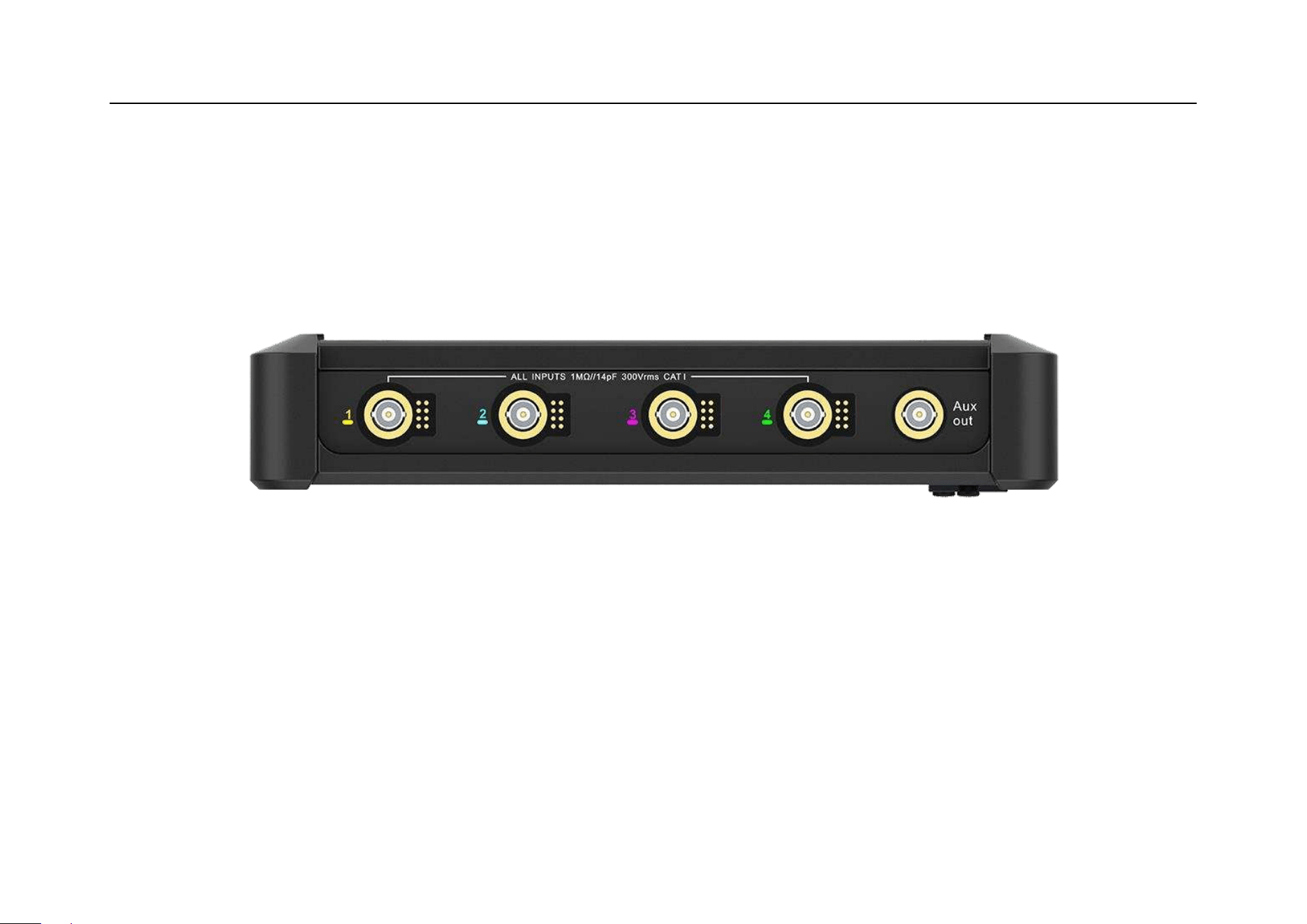
2.6 Front Panel
Figure 2-5 Front Panel of Automotive Oscilloscope

Chapter 2. Quick Start Guide of Oscilloscope
15
2.7 Power on/off the Oscilloscope
Power on/off the oscilloscope
First time start
Connect power adapter to the oscilloscope, and the oscilloscope should not be pressed on the adapter cable.
Check the Power-off lock on the side of oscilloscope and press the power button to start the instrument.
Power on
Press the power button to start the instrument while ensuring it is connected to a power supply.
Power off
Press the power button , go to power-off interface, and click to turn off the instrument.
Long press the power button for forced power-off of the instrument.
Power-off lock

16
Turn the power-off lock switch to OFF, the oscilloscope cannot be turned on.
Caution: Forced power-off may result in loss of unsaved data, please use with caution.
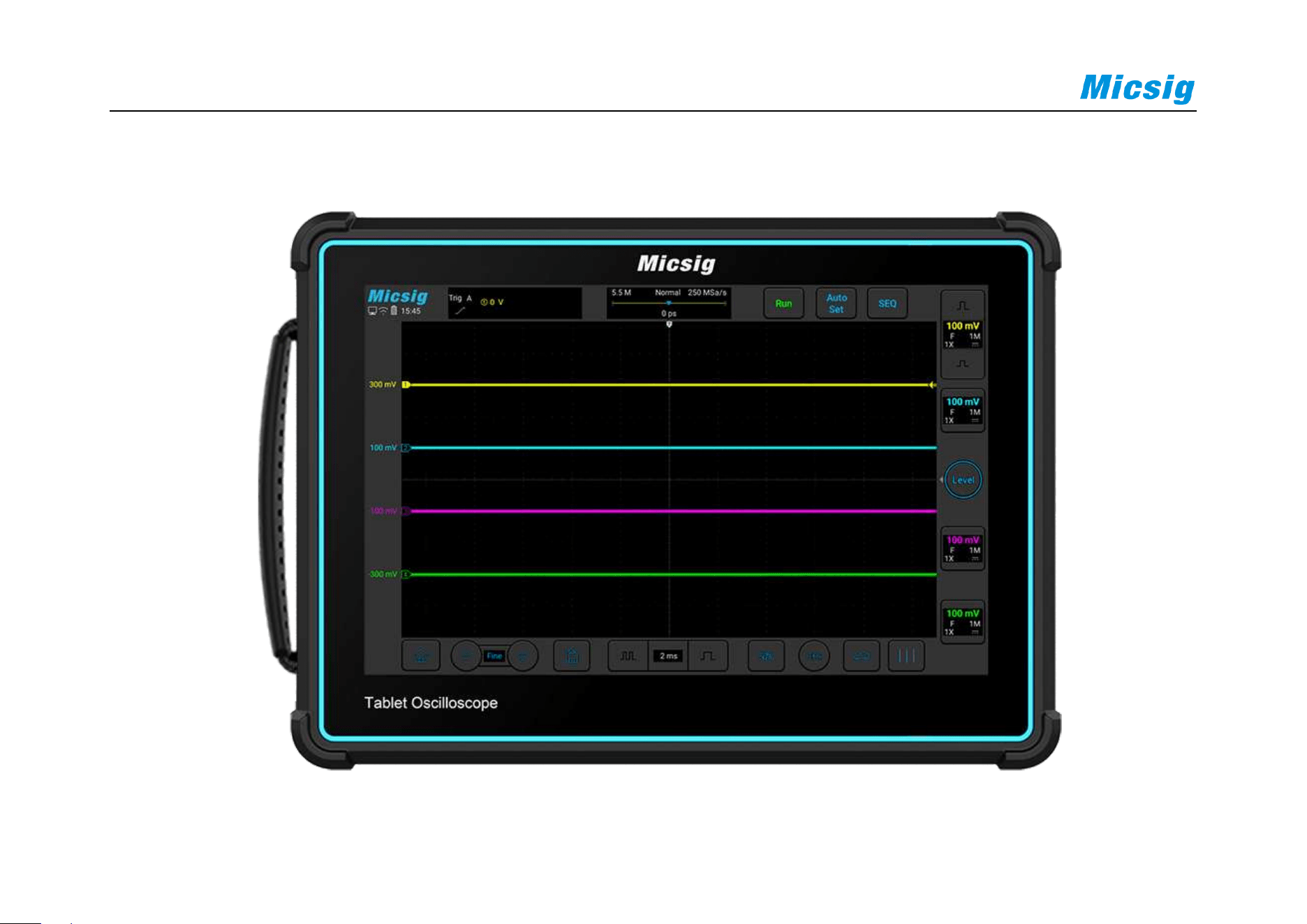
2.8 Understand the Oscilloscope Display Interface
This section provides a brief introduction and description of the ATO series oscilloscope user’s interface. After
reading this section, you can be familiar with the oscilloscope display interface content within the shortest possible
time. The specific settings and adjustments will be detailed in subsequent chapters and sections. The following
items may appear on the screen at a given time but not all items are visible. The oscilloscope interface is shown in
Figure 2-6.
Chapter 2. Quick Start Guide of Oscilloscope
17
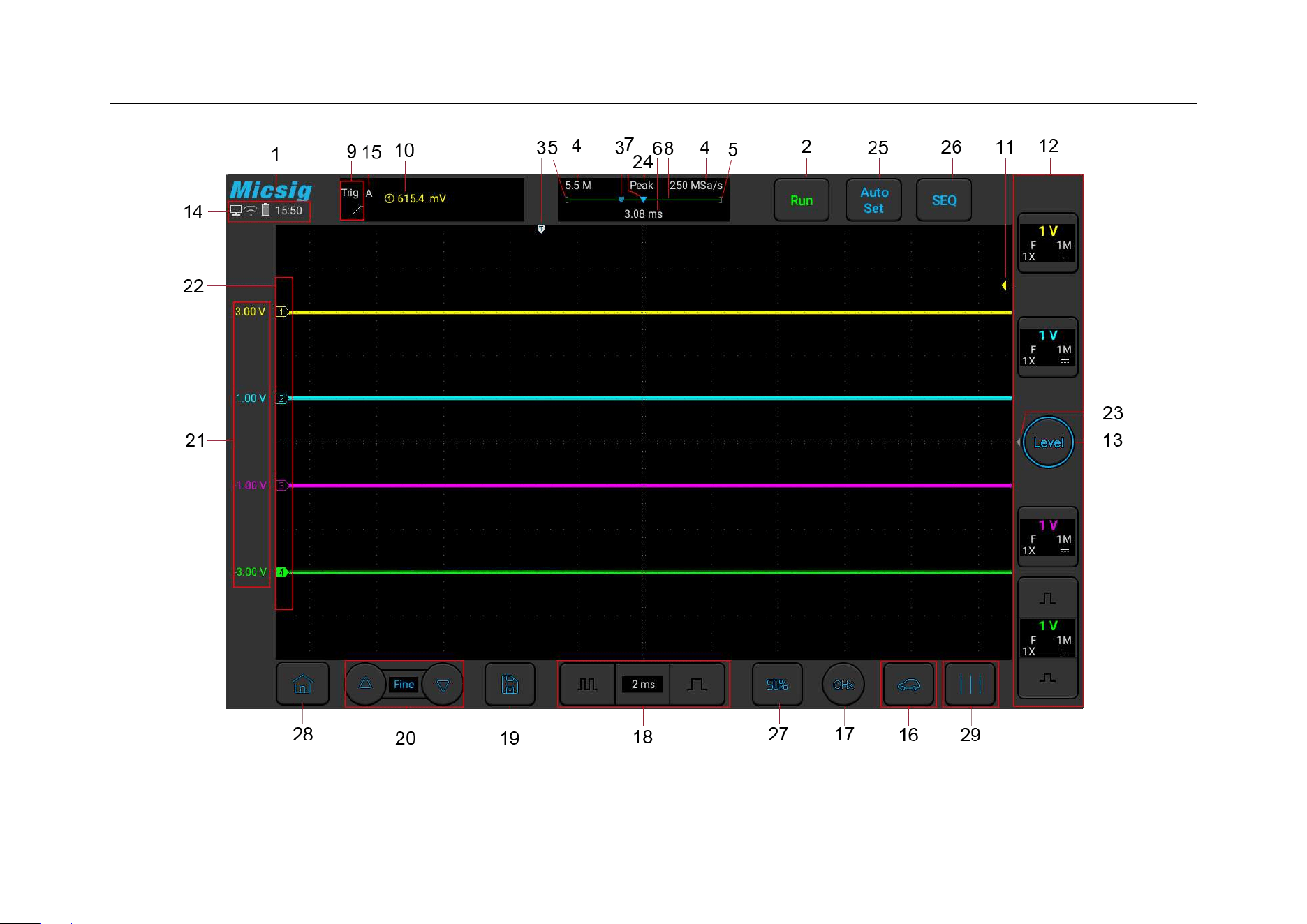
Figure 2-6 Oscilloscope Interface Display

18
No.
Description
1
Micsig logo
2
Oscilloscope status, including RUN, STOP, WAIT, Auto
3
Trigger point
4
Sampling rate, memory depth
5
The area in “[]” indicates the position of waveform displayed on the screen throughout the memory
depth
6
Delay time, the time at which the center line of the waveform display area is relative to the trigger
point
7
Center line of waveform display area
8
Memory depth indicatrix
9
Current trigger type indication
10
Current trigger source, trigger level

Chapter 2. Quick Start Guide of Oscilloscope
19
No.
Description
11
Trigger level indicator
12
CH1、CH2、CH3、CH4 channel icons and vertical sensitivity icon. Tap the channel icons to open
channels; Click or to adjust the vertical sensitivity of channels; Open the channel menu by
swipe left from the desired channel and swipe right to close; Display the vertical sensitivity of
channels; Display couple method.
13
Trigger level adjustment, press on the button to modify the trigger level through upward and
downward movements.
14
Display areas of USB-PC connection, USB connection, battery level, time etc.
15
Trigger Mode: A(auto), N(Normal).
16
Automotive diagnostic software presets
17
Current channel selection. Click to pop up the current channel switching menu to switch the current
channel.

20
No.
Description
18
Horizontal time base control icon. Tap the left/right time base buttons to adjust the horizontal time
base of the waveform. Tap the time base to open the time base table. Tap to select the desired time
base.
19
Quick save. Tap to quickly save the waveform as a reference waveform.
20
Fine adjustment button. Tap the button to finely adjust the last operation, including waveform
position, trigger level position, trigger point and cursor position.
21
The vertical position value of the channel indicator.
22
Channel indicator can indicate the zero-level position of the open channel.
23
Trigger quick start menu indicator: swipe left to open trigger quick start menu
24
Sample Mode: Normal, Average, Envelope, Peak
25
Auto Set, AutoRange
26
SEQ, Single Sequence Acquisition

Chapter 2. Quick Start Guide of Oscilloscope
21
No.
Description
27
50%: Touch to set:
The vertical position of the current channel waveform to the zero point
The horizontal position of the current channel waveform to center of the screen
The trigger level to the center of the trigger channel's waveform
The activecursor back to the center of the scree
28
Home
29
Phase rulers: help to measure the timing of a cyclic waveform on a scope view.
Table 2-1 Description of Oscilloscope Display Interface

22
2.9 Introduction Basic Operations of Touch Screen
The ATO series oscilloscope operates mainly by tap, swipe, single-finger drag.
Tap
Tap button on the touch screen to activate the corresponding menu and function. Tap any blank space on the screen
to exit the menu.
Swipe
Single-finger swipe: to open/close menus, including main menu, shortcut menu button and other channel menu
operations. For example, the main menu is opened as shown in Figure 2-7. The closing method is the opposite of
the opening method.
Chapter 2. Quick Start Guide of Oscilloscope
23
Figure 2-7 Slide out of Main Menu
Tap the options in the main menu to enter the corresponding submenu.

24
Single-finger drag
For coarse adjustments of vertical position, trigger point, trigger level, cursor, etc. of the waveform. Refer to “
4.1
Horizontal Move Waveform” and “5.3 Adjust Vertical Position” for details.
Pinch
For fine adjustments of vertical sensitivity.
2.10 Mouse Operation
Connect the mouse to the “USB Host” interface, then operate the oscilloscope with the mouse. The left button, right
button and scroll wheel of the mouse have the same functions as the finger touch function. Figure 2-8 is a schematic
diagram of the mouse single click to select “Run/Stop” function under the “Menu” option in the “Short-cut Menus”.
Chapter 2. Quick Start Guide of Oscilloscope
25
Figure 2-8 Mouse Cursor
2.11 Connect Probe to the Oscilloscope
1) Connect the probe to the oscilloscope channel BNC connector.
2)
Connect the retractable tip on the probe to the circuit point or measured equipment. Be sure to connect the
probe ground wire to the ground point of the circuit.

26
Maximum input voltage of the analog input
Category I 300Vrms, 400Vpk.
2.12 Use Auto
Once the oscilloscope is properly connected and a valid signal is input, tap the Auto Set button to quickly
configure the oscilloscope to be the best display effects for the input signal. While the oscilloscope in auto state, the
Auto Set button will light up .
Auto is divided into Auto Set and Auto Range. It is defaulted as Auto Set.
Auto Set — Single-time auto, and each time press “Auto”, the screen displays “Auto” in the upper left corner. The
oscilloscope can automatically adjust the vertical scale, horizontal scale and trigger setting according to the
amplitude and frequency of signals, adjust the waveform to the appropriate size and display the input signal. After
adjustments, exit from the auto set, the “Auto” in the upper left corner disappears.
Channels may be automatically opened. Any channel greater or less than the threshold level can be opened or
closed automatically according to the set threshold level. The threshold level can be settable.
Chapter 2. Quick Start Guide of Oscilloscope
27
Source can be automatically triggered, and the triggered source channel can be automatically set to select priority to
the current signal or to the maximum signal.
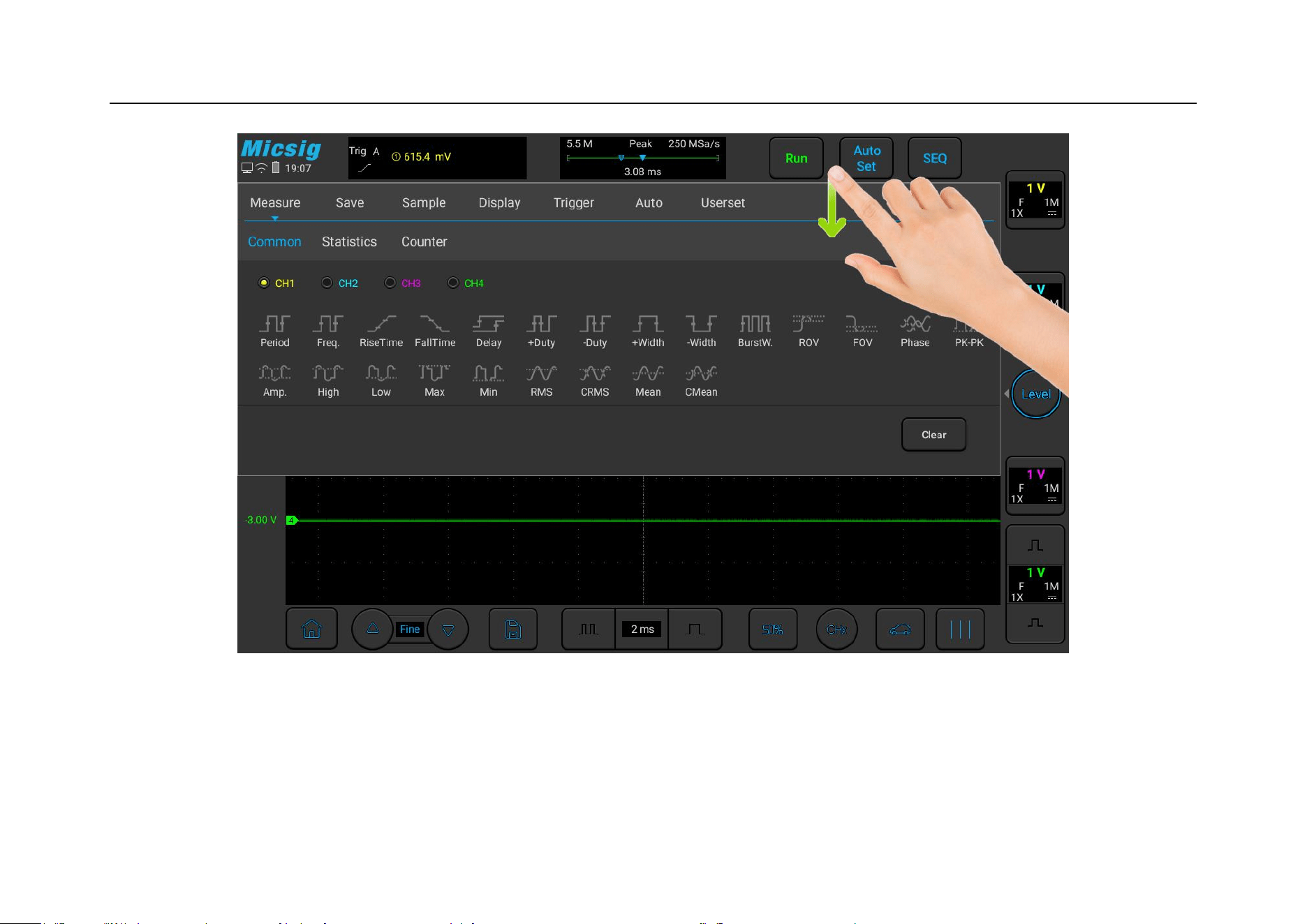
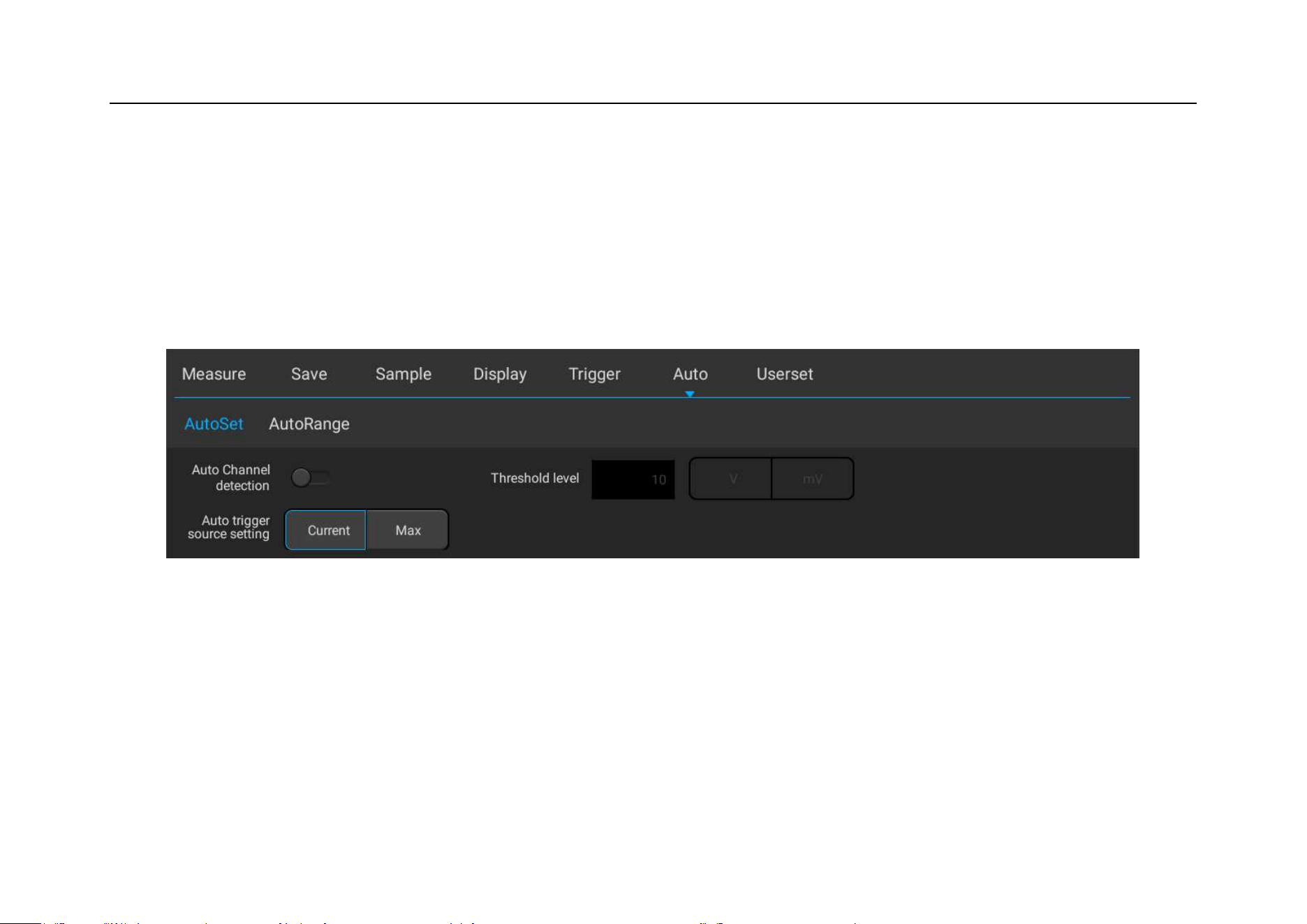
Open the main menu. Tap “Auto” to open the auto set menu, including channel open/close setting, threshold voltage
setting and trigger source setting.
Figure 2-9 Open Auto Set
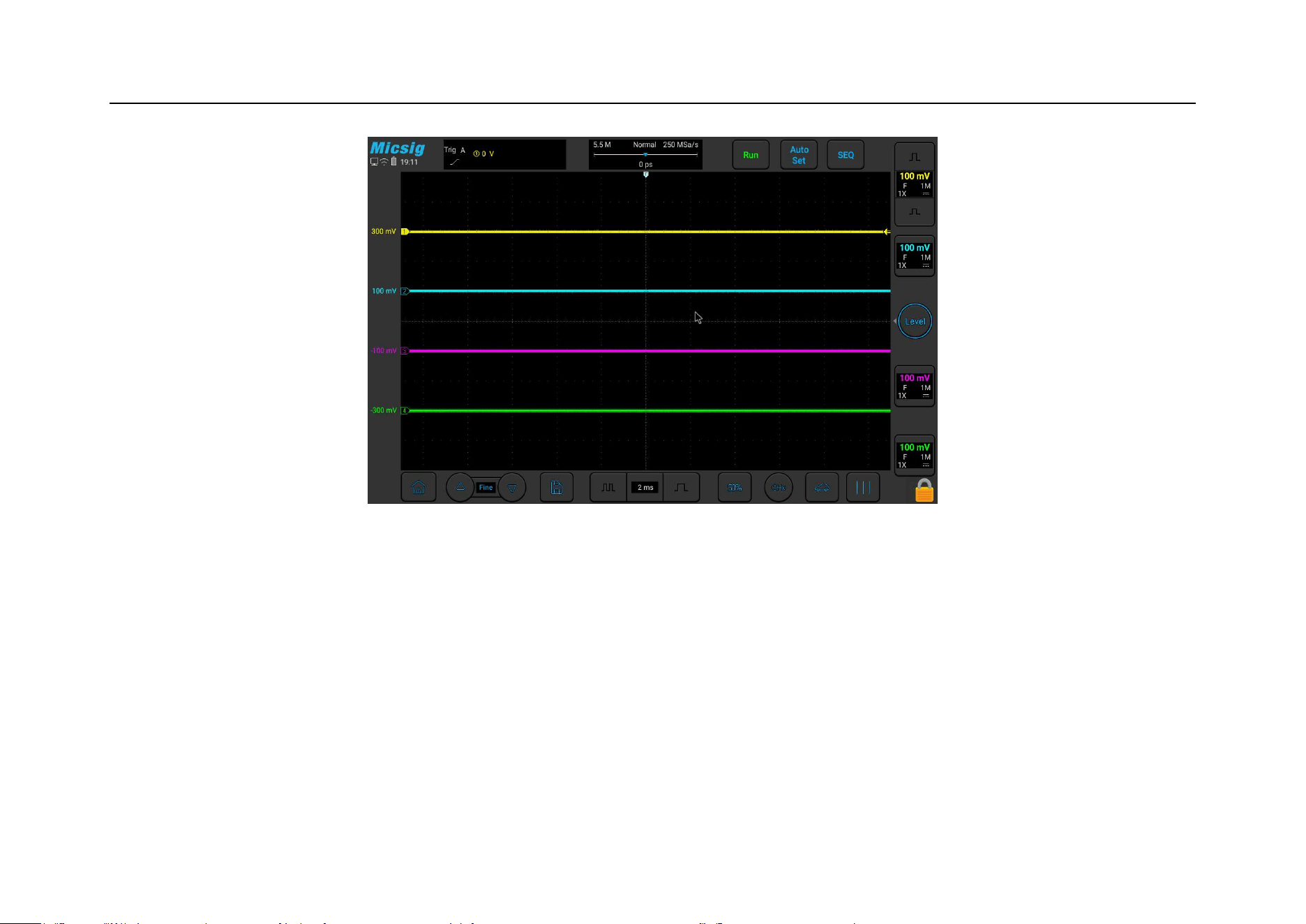
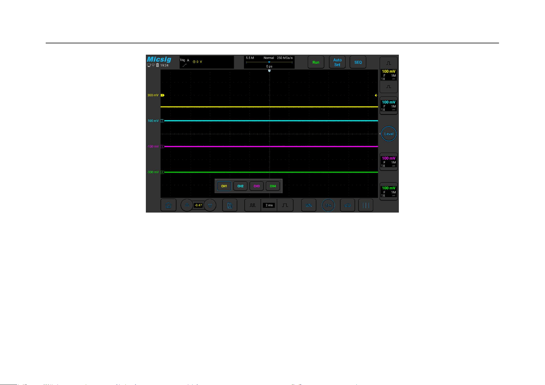
Automatic configuration includes: single channel and multiple channels; automatic adjustment of the horizontal
time base, vertical sensitivity and trigger level of signal; the oscilloscope waveform is inverted off, the bandwidth
limit sets to full bandwidth, it sets as DC coupling mode, the sampling mode is normal; the trigger type is set to
edge trigger and the trigger mode is automatic.
28
Note: The application of Auto Set requires that the frequency of measured signal is no less than 20Hz, the duty ratio
is greater than 1% and the amplitude is at least 2mVpp. If these parameter ranges are exceeded, Auto Set will fail.
Figure 2-10 Auto Set Waveform
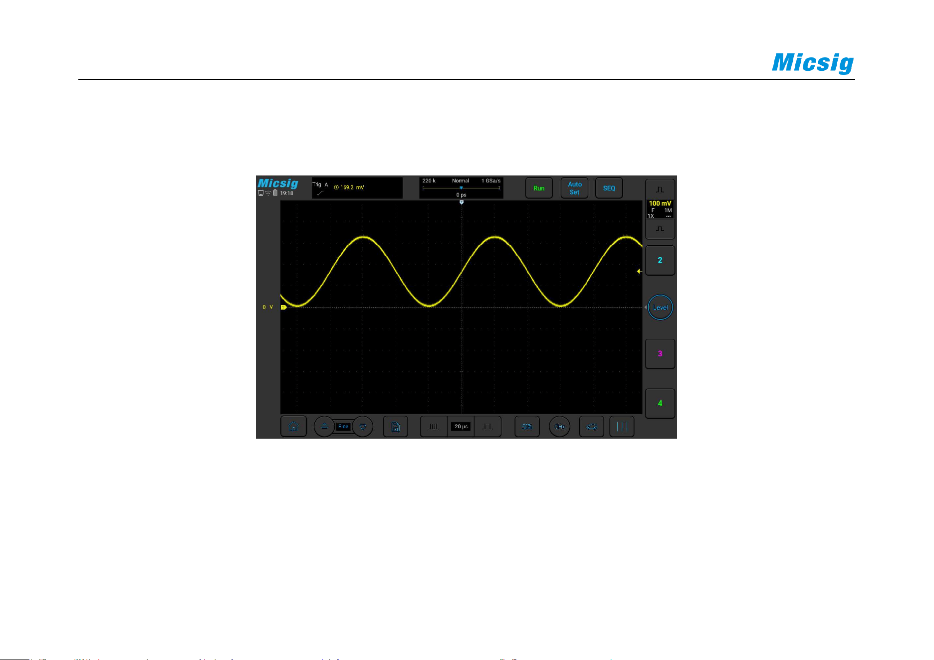
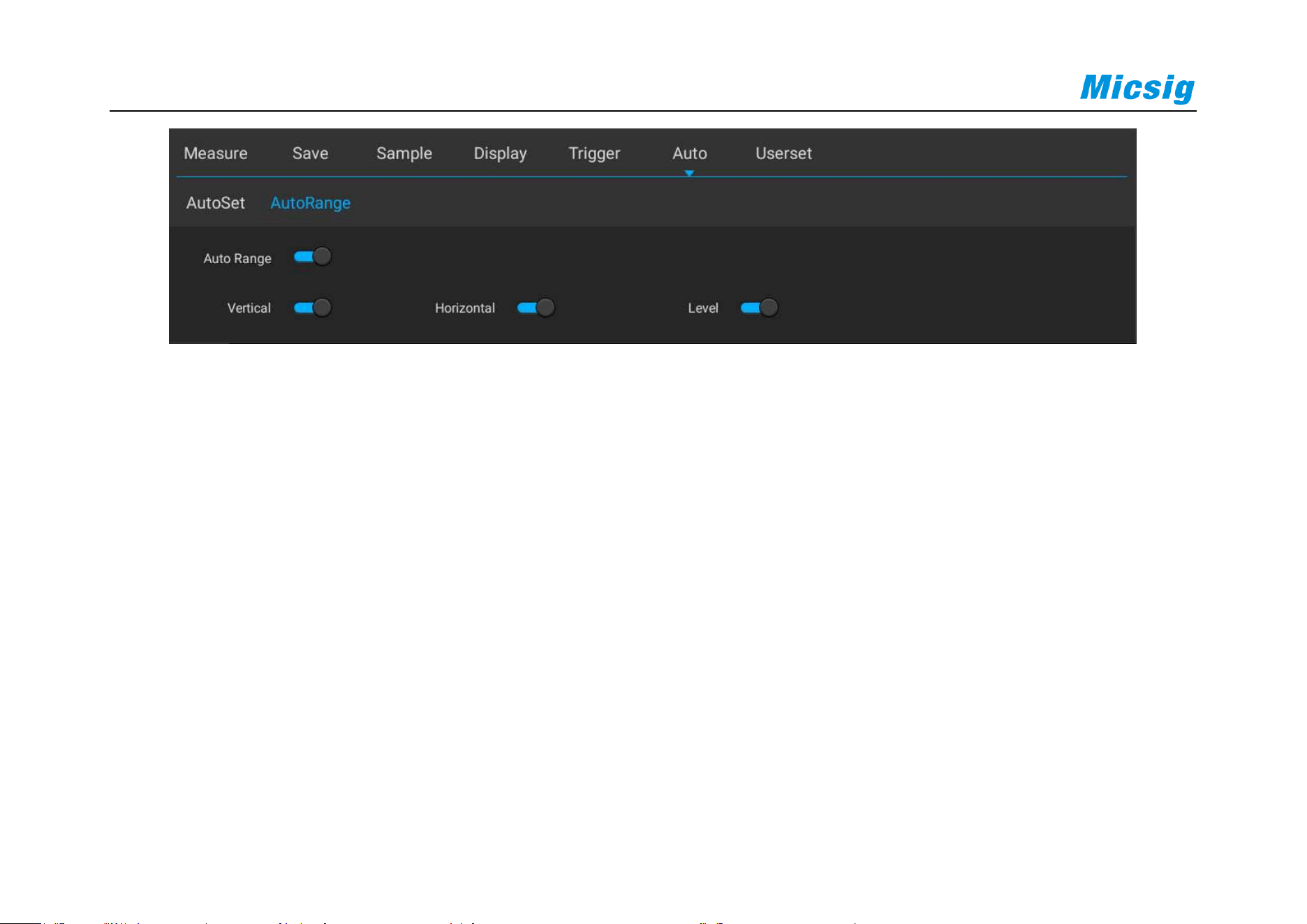
Auto Range - Continuously automatic, the oscilloscope continuously adjusts the vertical scale, horizontal time base
and trigger level in a real-time manner according to the magnitude and frequency of signal. It is defaulted as off and
needs to be opened in the menu. This function is mutually exclusive with “Auto Set”.

Chapter 2. Quick Start Guide of Oscilloscope
29
Open the main menu and tap “Auto” to open the auto range menu for the corresponding settings. When the
oscilloscope auto range function is turned on, the oscilloscope will automatically set various parameters, including:
vertical scale, horizontal time base, trigger level, etc. When the signal is connected, these parameters will
automatically change, and the signal does not need to be operated again after the change. The oscilloscope will
automatically recognize and make the appropriate changes.
Auto range: Turn the auto range function on or off
Vertical scale: Turn on the vertical scale automatic adjustment function;
Horizontal time base: Turn on the horizontal time base automatic adjustment function;
Trigger level: Turns on the auto-adjust trigger level function.
30
Figure 2-11 Open Auto Range
Auto Range is usually more useful than Auto Set under the following situations:
1) It can analyze signals subject to dynamic changes.
2) It can quickly view several continuous signals without adjusting the oscilloscope. This function is very useful
if you need to use two probes at the same time, or if you can only use the probe with one hand because the
other hand is full.
3) Control the automatic adjustment setting of the oscilloscope.

Chapter 2. Quick Start Guide of Oscilloscope
31
2.13 Load Factory Settings
Open the main menu, tap “User Settings” to enter the user setting page. Tap “Factory Settings” and the dialog box
for loading factory settings will pop-up. Press “OK” and load the factory settings. The dialog box for loading
factory settings is shown in Figure 2-12.
Figure 2-12 Load Factory Settings
2.14 Use Auto-calibration
Open the main menu, tap “Userset” to enter the user setting page. Tap “Self Adjust” to enter the auto-calibration
mode. When the auto-calibration function is active, the upper left corner of the screen displays “Calibrating” in red,

32
and after calibrating is finished, the word in red disappears. When the temperature changes largely, the auto-
calibration function can make the oscilloscope maintain the highest accuracy of measurement.
Auto-calibration should be done without probe.
Auto-calibration process takes about two minutes.
If the temperature changes above 10℃, we recommended users perform the auto-calibration.
Manual zero calibration- The oscilloscope supports manual zero calibration for each channels. Click the "Fine"
button in the lower left corner would open the forced channel selection menu and display the offset value, select the
channel to be adjusted, and slide the waveform up and down to manually adjust the zero position. Tap“△”,
“▽”button can fine-tune the zero position, as shown in Figure 2-13
Chapter 2. Quick Start Guide of Oscilloscope
33
Figure 2-13 Manual zero calibration
2.15 Passive Probe Compensation
Before connecting to any channels, users should make a probe compensation to ensure the probe match the input
channel. The probe without compensation will lead to larger measurement errors or mistakes. Probe compensation

34
can optimize the signal path and make measurement more accurate. If the temperature changes 10℃ or above, this
program must run to ensure the measurement accuracy.
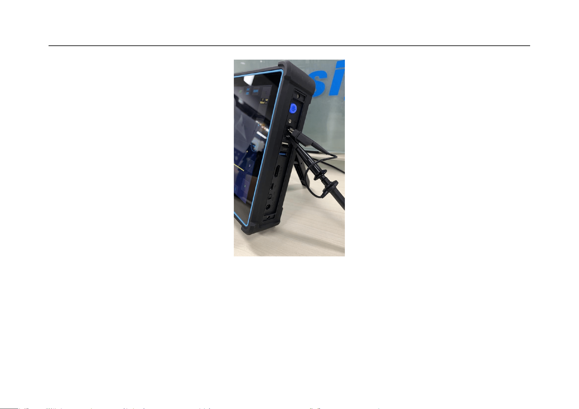
Probe compensation may be conducted in the following steps:
1) First, connect the oscilloscope probe to CH1. If a hook head is used, make sure that it is in good connection
with the probe.
2) Connect the probe to the calibration output signal terminal and connect the probe ground to the ground
terminal. As shown in Figure 2-13.
Chapter 2. Quick Start Guide of Oscilloscope
35
Figure 2-13 Probe Connection
3) Open the channel (if the channel is closed).
4) Adjust the oscilloscope channel attenuation coefficient to match the probe attenuation ratio.
36
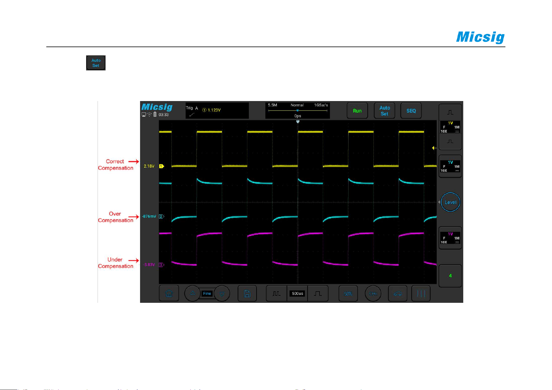
5) Tap button or manually adjust the waveform vertical sensitivity and horizontal time base. Observe the
shape of the waveform, see Figure 2-14.
Figure 2-14 Probe Compensation
Chapter 2. Quick Start Guide of Oscilloscope
37
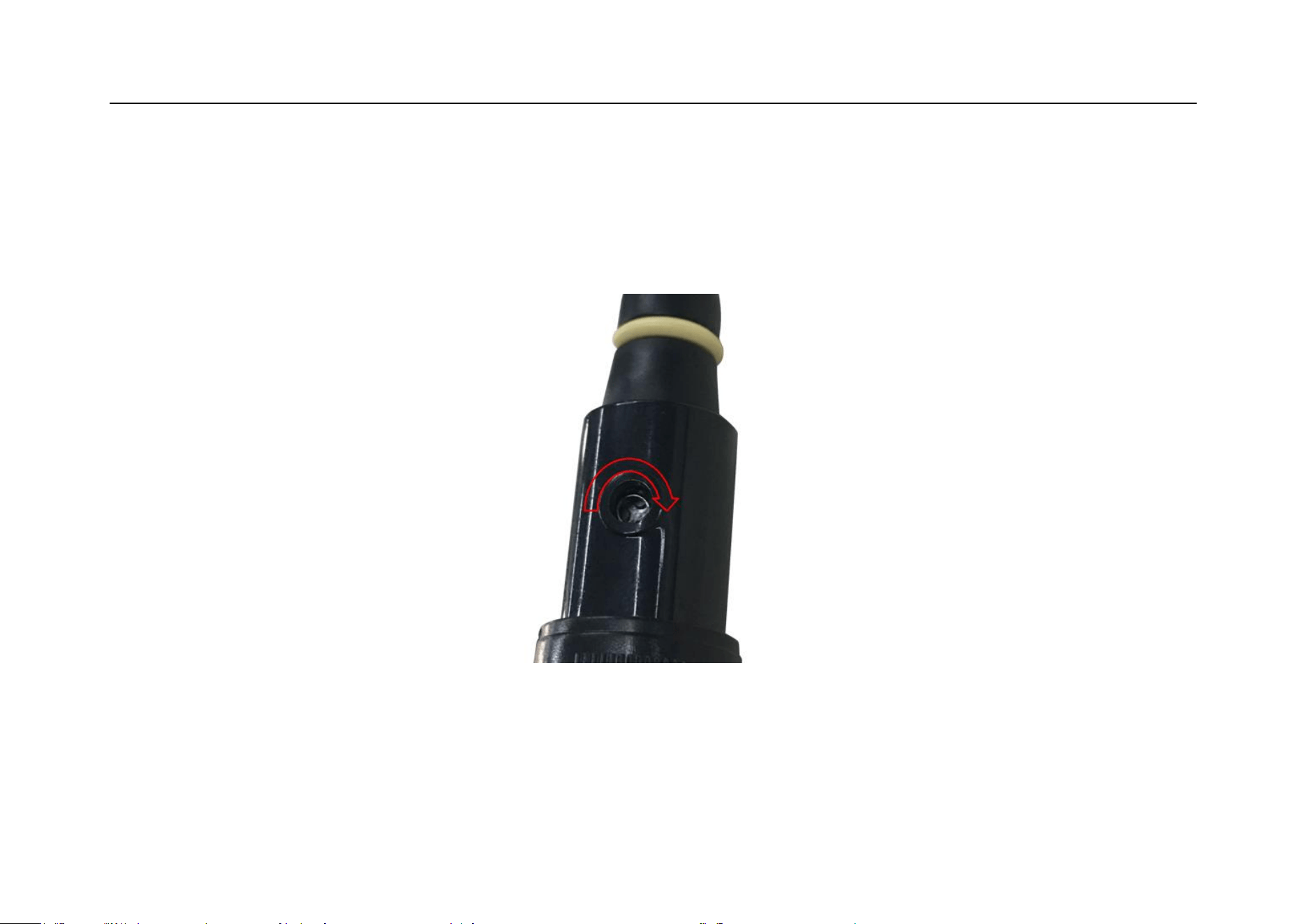
If the waveform on the screen is shown as “under-compensation” or “over-compensation”, please adjust the
trimmer capacitor until the waveform shown on the screen as “correct-compensation”. The probe adjustment is
shown in Figure 2-15.
Figure 2-15 Probe Adjustment
The safety ring on the probe provides a safe operating range. Fingers should not exceed the safety ring when using
the probe, so as to avoid electric shock.

38
6) Connect the probe to all other oscilloscope channels (Ch2 of a 2-channel oscilloscope, or Ch 2, 3 and 4 of a 4-
channel oscilloscope).
7) Repeat this step for each channel.
Warning
Ensure the wire insulation is in good condition to avoid probe electric shock while measuring high voltage.
Keep your fingers behind the probe safety ring to prevent electric shock.
When the probe is connected a voltage source, do not touch metal parts of the probe-head to prevent electric
shock.
Before any measurement, please correctly connect the probe ground end.
2.16 Modify the Language
To modify the display language, please refer to “
14.3 Settings - Language and Input Method”.

Chapter 3 Automotive Test
39
Chapter 3 Automotive Test
This chapter contains most of the test applications of ATO automotive oscilloscopes in automotive circuits. The
purpose is to help users quickly troubleshoot and locate automotive electronics faults. It is recommended that you
read this chapter carefully to understand the general operation and use of automotive oscilloscopes.
3.1 Charging/Start Circuit
All electrical equipment of the car is powered by a power system composed of an on-board generator and a battery.
In this power system, the generator supplies power to the electrical equipment and charges the battery when the
generator is working normally. When the power generated by the generator is less than the power consumed by the
on-board electrical equipment, the battery participates in power supply to make up for its deficiency. When the
engine is working normally, it is necessary to ensure sufficient charging time for the battery to ensure that it does
not lose power. When the generator is working normally, whether to charge the battery can be indicated from the
charging indicator on the instrument panel. Due to the large speed range of the engine, the generator must be
equipped with a voltage regulator to ensure that its rated voltage is not affected by the speed and current. The power
40
supply when the engine starts is completely provided by the battery, so the battery must ensure that there is enough
capacity to start the engine smoothly. The ATO series car-specific oscilloscope can test the charging circuit and the
starting circuit to test whether the charging/starting circuit of the car is working properly. The specific operations
are as follows::
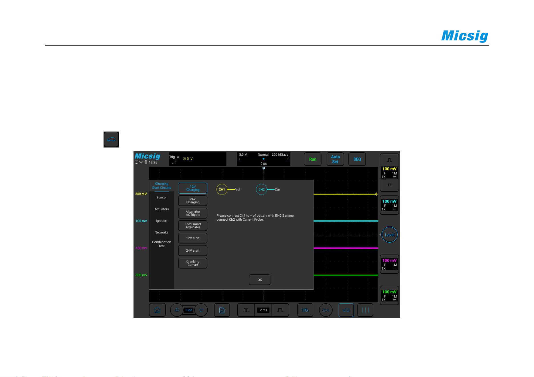
Click the icon in the lower right corner of the oscilloscope to display the screen shown in Figure 3-1:
Figure 3-1 Charging/Start Circuits

Chapter 3 Automotive Test
41
3.1.1 12V Charging
12V charging is suitable for gasoline vehicles. Use a BNC to banana cable, one end is connected to channel 1 of the
oscilloscope, and the other end is connected to the positive and negative electrodes of the battery using two large
alligator clips (the red wire is connected to the red clip to the positive electrode, and the black wire is connected to
the black clip. negative electrode). If you need to measure current, please use a current clamp of 600A and above,
connect the BNC of the current clamp to channel 2, turn on the switch of the current clamp, and clamp the current
clamp to the output power line of the generator.
The alternator provides power to the vehicle. There is little difference between different manufacturers. The
charging voltage is generally between 13.5V and 15.0V. It is not good if it is too large or too small. The output
current of the generators of different models of different manufacturers is not the same, so it needs to be estimated
according to the vehicle.
42
Note: The generator adopts AC power generation. The voltage is converted to DC through multiple rectifier diodes.
The voltage can be measured by a multimeter. However, when the diodes are damaged, the multimeter displays the
correct readings, and the waveform can be judged by an oscilloscope.
The specific operation is shown in Figure 3-2:
Figure 3-2 12V Charging
Chapter 3 Automotive Test
43
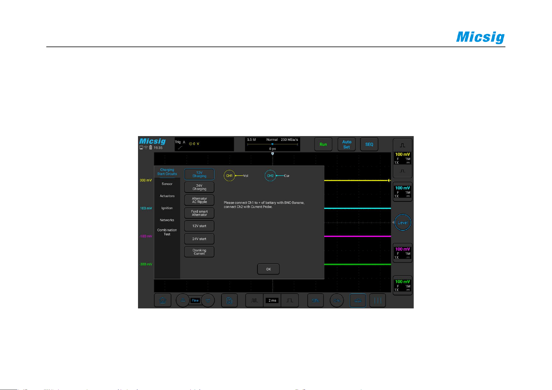
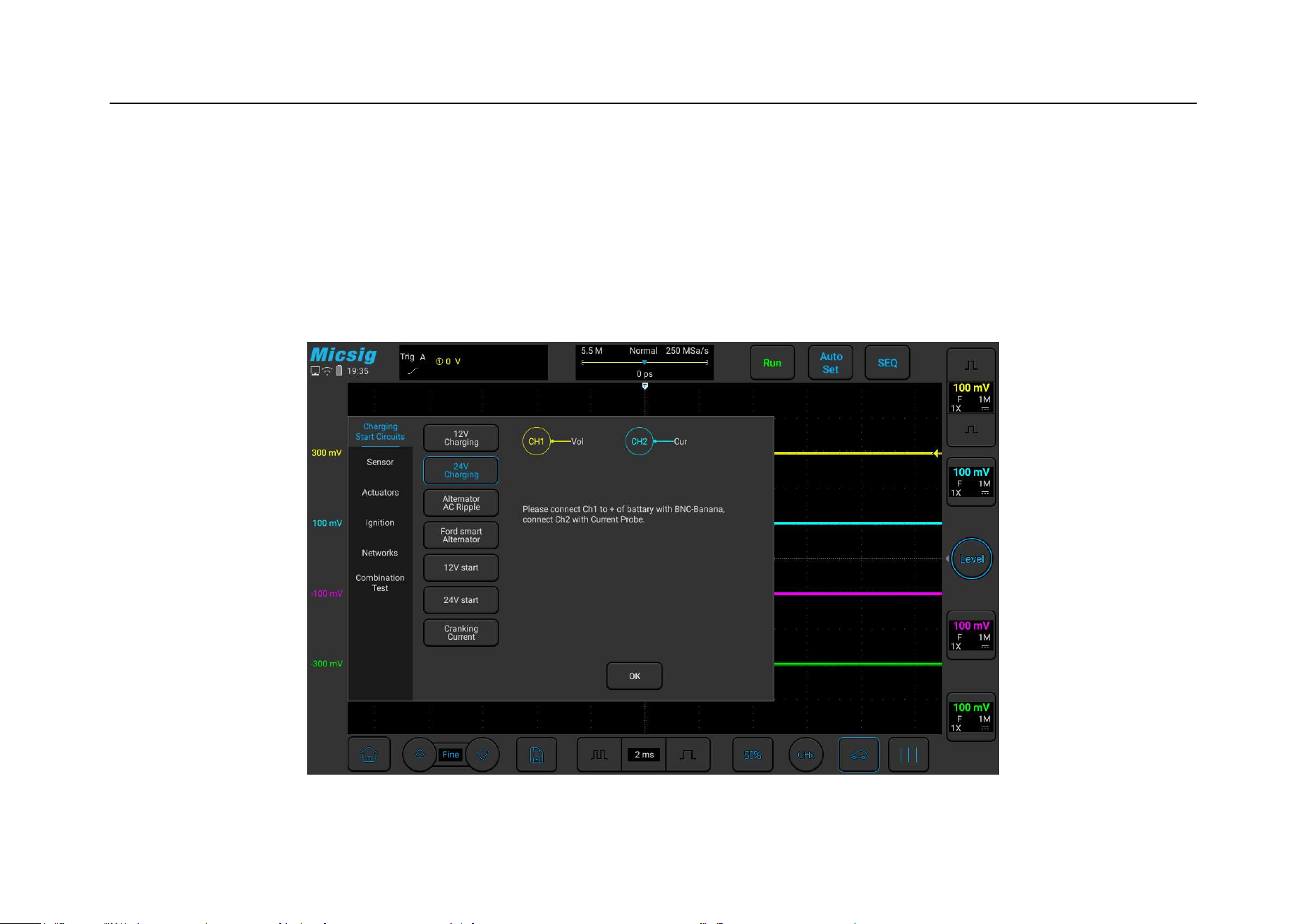
3.1.2 24V Charging
24V charging is suitable for diesel vehicles. The operation process is the same as that of 12V charging. The
reference voltage is 26.5V~30V. It can be tested with an oscilloscope. The specific operation is shown in Figure 3-
3:
Figure 3-3 24V Charging

44
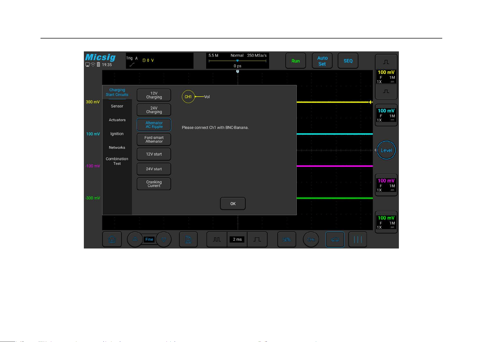
3.1.3 Alternator AC Ripple
The ATO oscilloscope can test the charging ripple and assist the user to determine whether the charging process is
normal. Use a BNC to banana cable, one end is connected to the oscilloscope channel 1, and the other end is
clamped between the positive and negative electrodes of the battery (the red wire is connected to the red clip)
Connect the positive pole, and connect the black wire to the black clip to the negative pole). Start the vehicle and
start the test. At this time, the oscilloscope is coupled to AC, and what is displayed is not the true voltage value. It is
based on the DC waveform and the difference relative to the DC voltage.
As shown in Figure 3-4 below:
Chapter 3 Automotive Test
45
Figure 3-4 Charging Ripple

46
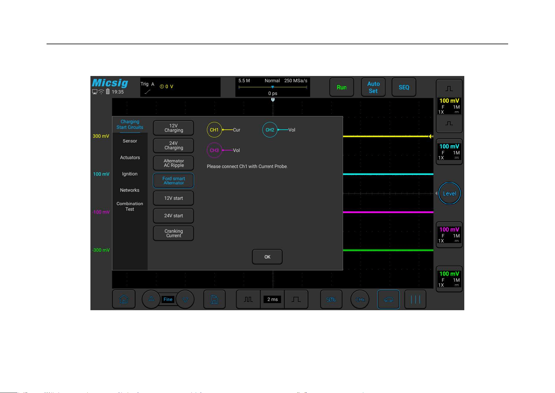
3.1.4 Ford Focus Smart Generator
Use a BNC to banana cable, connect one end to channel 1 of the oscilloscope, connect the black plug to the black
alligator clip to ground (battery negative), and use a needle to connect the red connector to the engine ECM to
generator output control line. Use BNC to banana cable, one end Connect to channel 2 of the oscilloscope, the other
black plug is connected to the black alligator clip to ground (the negative electrode of the battery), and the red
connector is connected to the feedback of the generator to the engine ECM with a stinger.
Use a current clamp of 600A and above, connect the BNC of the current clamp to channel 3, turn on the switch of
the current clamp, and clamp the current clamp to the output power line of the generator.
Start the vehicle and start the test. Among them, the control signal of ECM to the generator on channel 1 is square
wave/pulse width modulation signal/LIN line; the feedback signal of the generator on channel 2 is square
wave/pulse width modulation signal, which is displayed on channel 3. Is the output current of the generator.
Chapter 3 Automotive Test
47
Use the ATO oscilloscope to test the Focus smart generator, the specific operation is shown in Figure 3-5:
Figure 3-5 Ford Focus Smart Generator

48
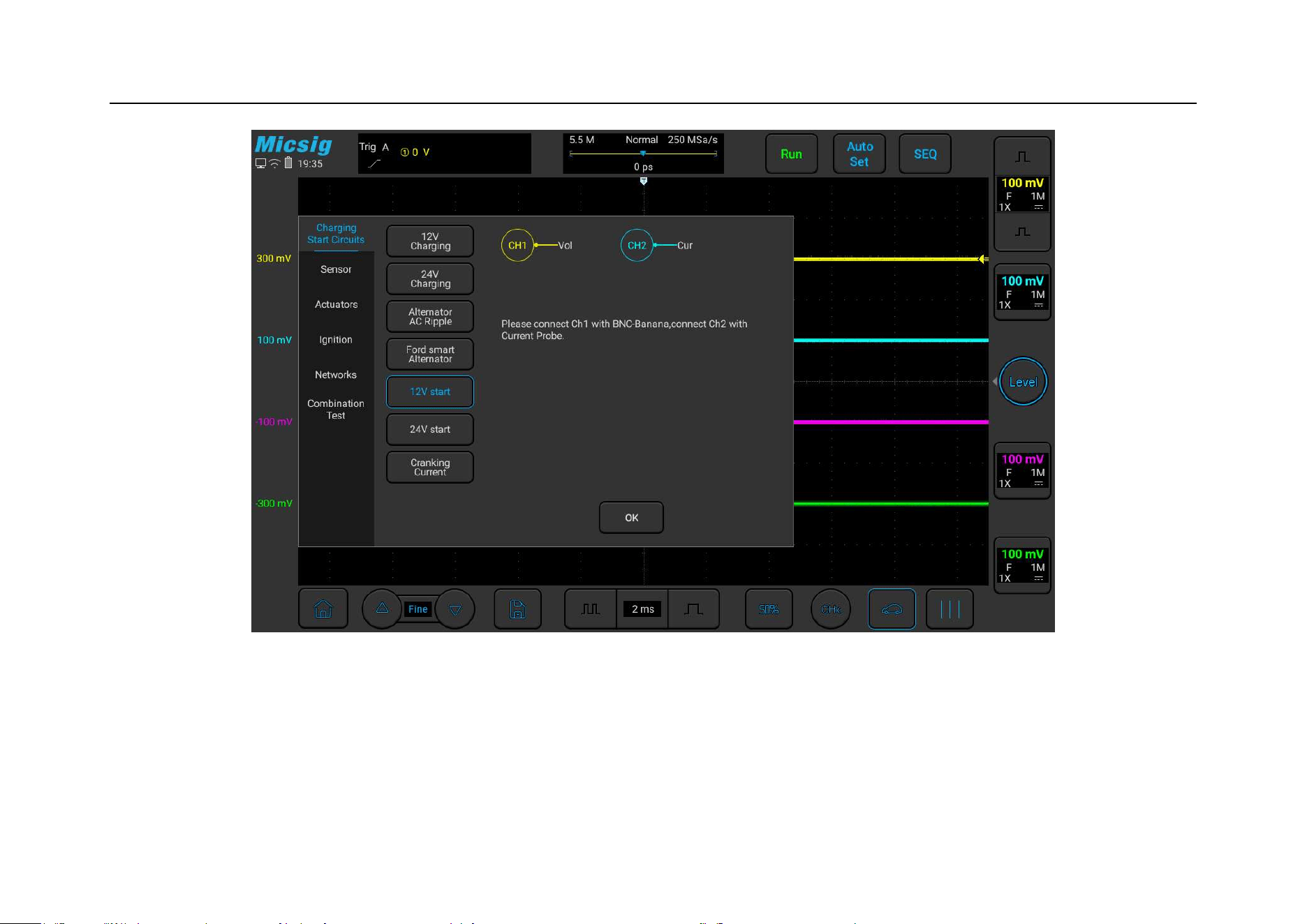
3.1.5 12V Start
Use the ATO oscilloscope to test the start of the gasoline car, the purpose is to test whether the performance of the
battery is maintained in the normal range. Use a BNC to banana cable, connect one end to channel 1 of the
oscilloscope, and use two large alligator clips to clamp the positive and negative poles of the battery (the red wire
connects to the red clamp to the positive pole, and the black wire to the black clamp to the negative pole). Use a
current clamp above 600A, connect the BNC of the current clamp to channel 2, turn on the switch of the current
clamp, and clamp the current clamp to the positive or negative power line of the battery. You need to clamp the
entire positive or negative line. Stay, pay attention to the positive and negative polarity (positive current flows from
the positive to the negative of the battery). The specific operation is shown in Figure 3-6:
Chapter 3 Automotive Test
49
Figure 3-6 12V Start
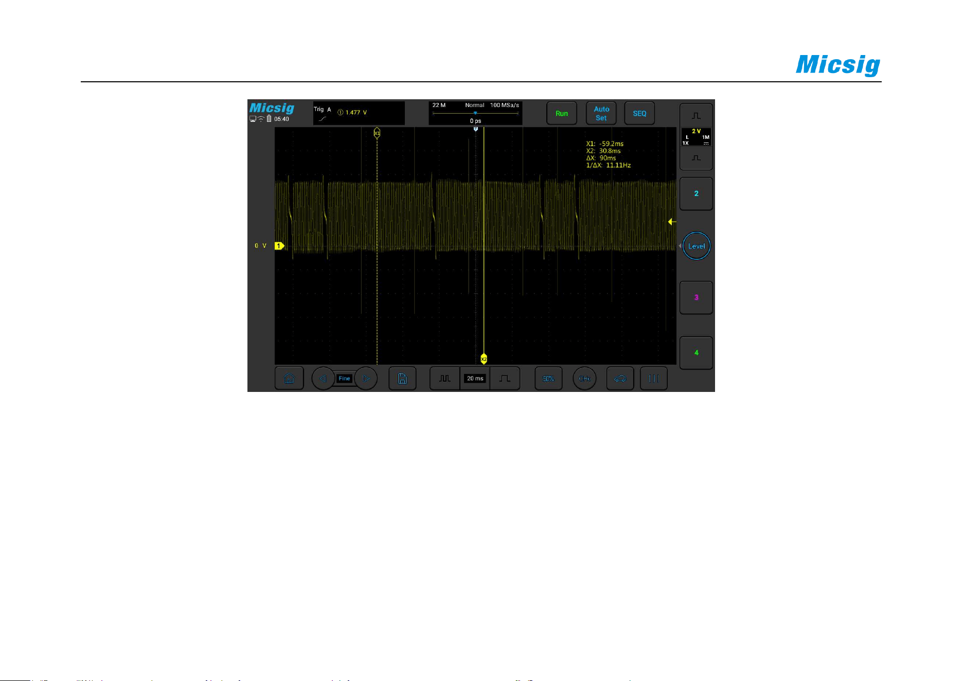
The following figure is the actual measurement diagram of the starting voltage and current of Mazda in a certain
year:
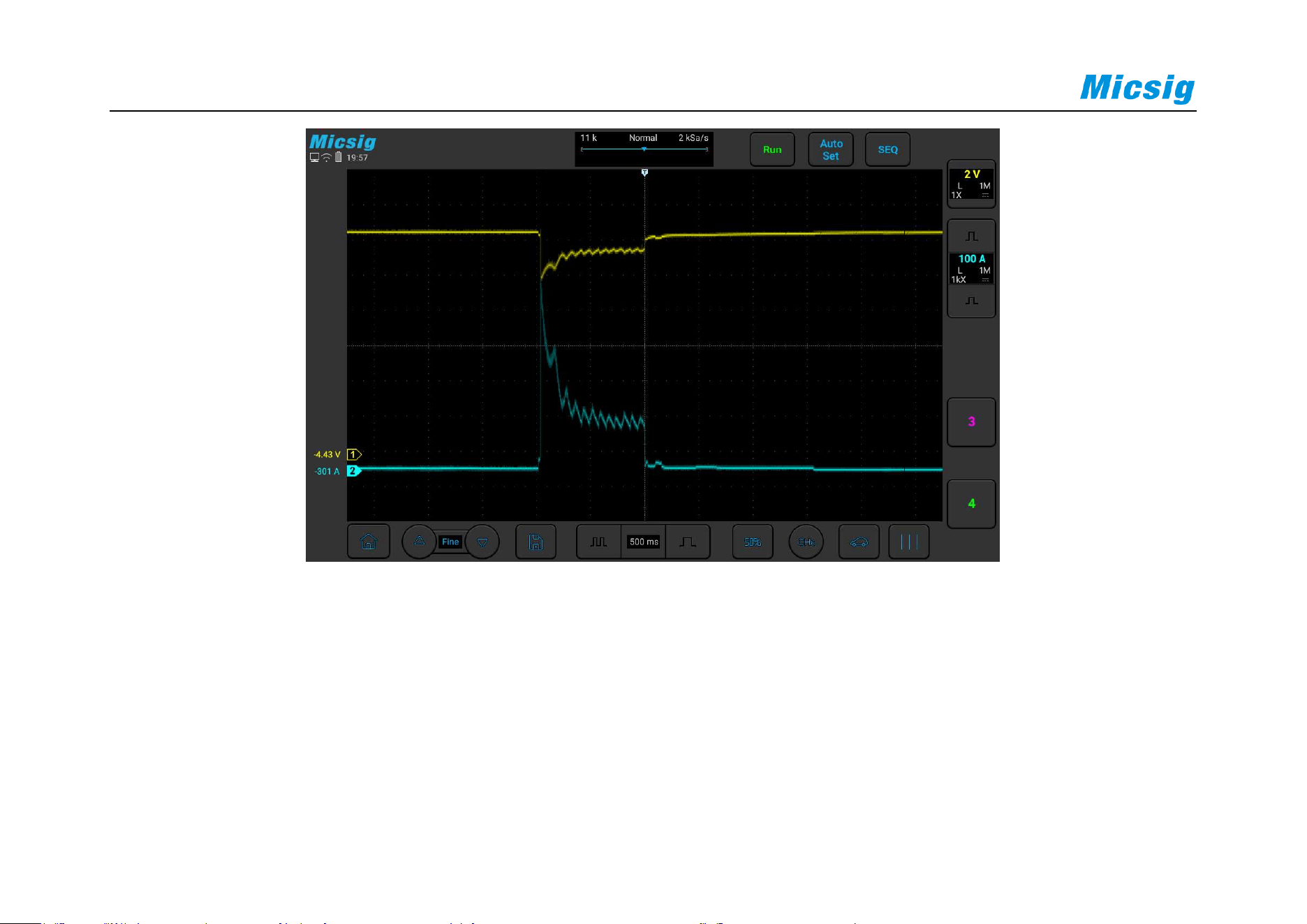
50
Figure 3-7 Starting voltage and current
3.1.6
24V Start
Use the ATO oscilloscope to test the starting process of the diesel vehicle, the purpose is to test whether the
performance of the battery is maintained in the normal range, the operation process is the same as the 12V start. The
specific operation is shown in Figure 3-8:
Chapter 3 Automotive Test
51
Figure 3-8 24V Start
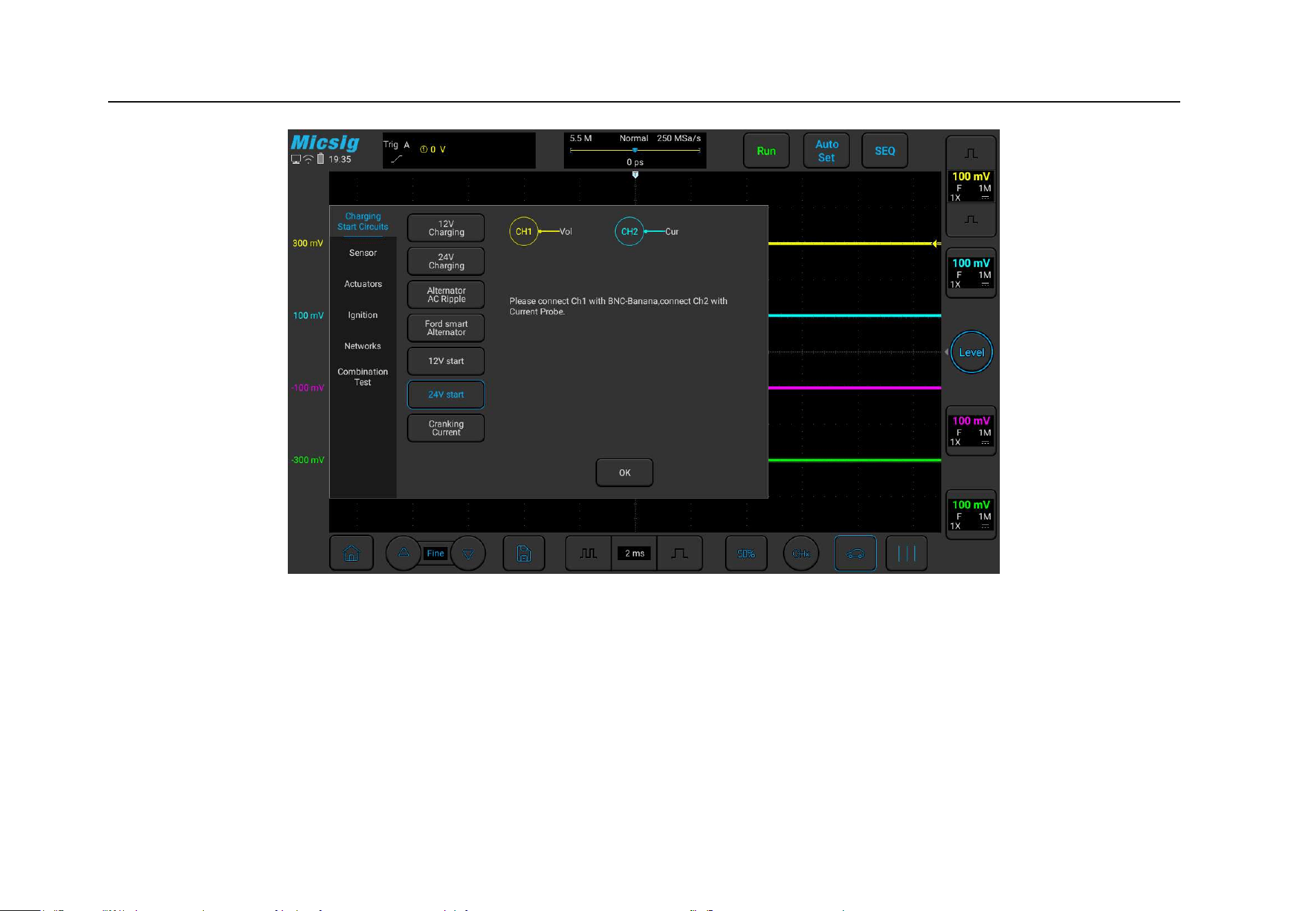
3.1.7
Cranking Current
Use an ATO oscilloscope with a current probe to conduct a current test on the starting process of the car
(automobile or diesel car), observe whether the current waveform is normal, use a current clamp of 600A or above,
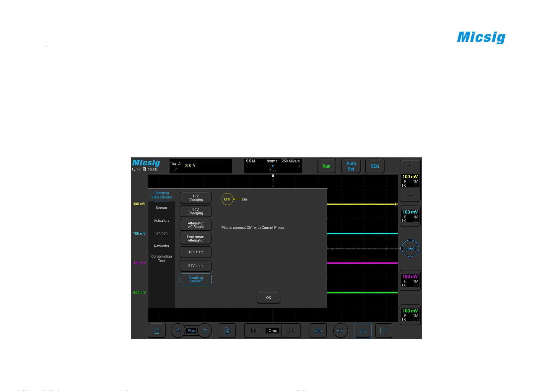
52
and connect the BNC of the current clamp to channel 2. On, turn on the switch of the current clamp and clamp the
current clamp to the positive or negative power line of the battery. You need to clamp the entire positive or negative
line. Pay attention to the positive and negative polarity (positive current flows from the positive electrode of the
battery to the negative electrode).
The specific operation is shown in Figure 3-9:
Figure 3-9 Cranking Current

Chapter 3 Automotive Test
53
3.2 Sensor Tests
The sensor is an electronic signal conversion device that converts non-electrical information into voltage signals
and reports various information about changes in the working environment to the car computer. For example, the air
flow meter installed between the air filter and the throttle valve can measure the value of the air flow that is sucked
into the engine through the throttle valve. It converts the air flow value into a voltage signal and sends it to the
engine ECU (control computer), the control computer adjusts the corresponding fuel injection volume according to
the change of air flow to achieve the goal of the best combustion ratio. Another example is a vehicle speed sensor.
Its function is to convert the vehicle speed into a voltage signal and send it to the trip computer. The trip computer
controls the shift timing to achieve upshift or downshift.
With the continuous development of cars in the direction of intelligence and new energy, the number of sensors on
the car body has shown a trend of sharp increase, and there are nearly 100 sensors on the mid-to-high-end cars of
the company. The ATO series special oscilloscope can directly measure the signal waveform of the sensor. By
comparing with the standard waveform during normal operation, it is easy to find whether the sensor is normal. The

54
ATO series oscilloscope can test the following types of sensors. The purpose is to compare the real-time waveforms
with the standard waveforms to help users find problems. The following are expanded and explained separately:
3.2.1
ABS
The ABS wheel speed sensor is divided into analog and digital. The analog sensor has 2 signal terminals, the signal
is a sine wave, and the frequency of the sine wave represents the speed. Digital sensors generally have 3 terminals,
power, signal, and ground; the signal line needs to be tested, the signal is a square wave pulse, and the square wave
frequency represents the speed.
When testing, use BNC to banana cable, the BNC head is connected to the oscilloscope, and the banana head is
connected to the sensor or the ECM pin to test 1/2/4 signals at the same time. Shown as Figure 3-10:
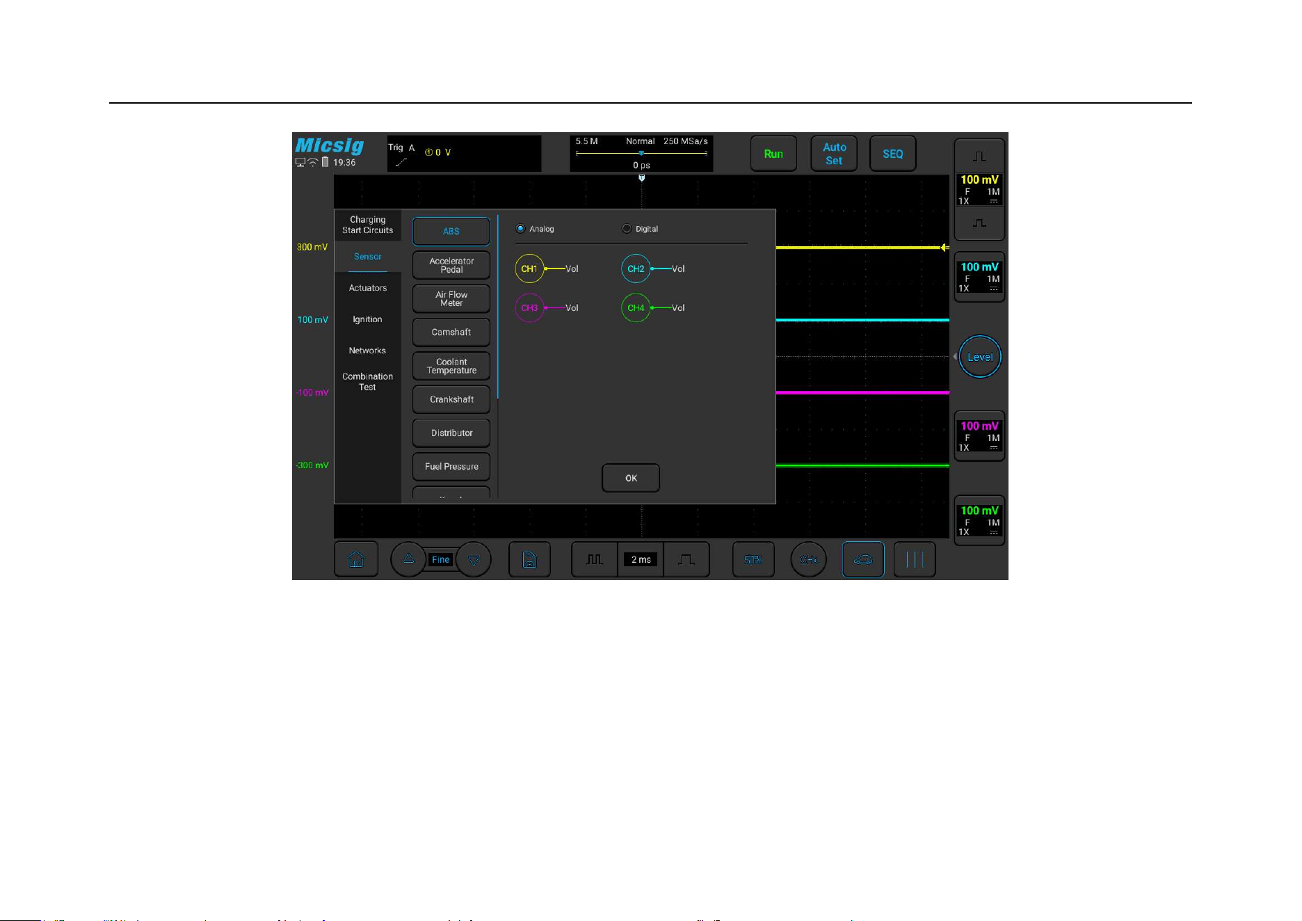
Chapter 3 Automotive Test
55
Figure 3-10 ABS Wheel Speed Sensor
3.2.2
Accelerator pedal
The accelerator pedal is the signal of the automobile accelerator. There are generally 2 groups, each pair of 3 wires,
power, signal, and ground. Divided into analog/analog and analog/digital. Analog/analog signal is two analog

56
signals, usually there are two ways, one is deviation signal: one signal is from 0.3V→4.8V, which rises as the
accelerator pedal is depressed, and the other is 4.8V→0.3V, with Depress the accelerator pedal and descend. The
other is the same direction signal, but the voltage is different, one is 0.5V→2.5V, the other is 1V→4.5V; (the
voltage range is for reference only, the voltage range may be slightly different for different models, but the trend is
the same).
Use ATO oscilloscope to test the accelerator pedal sensor, the specific operation is shown in Figure 3-11:
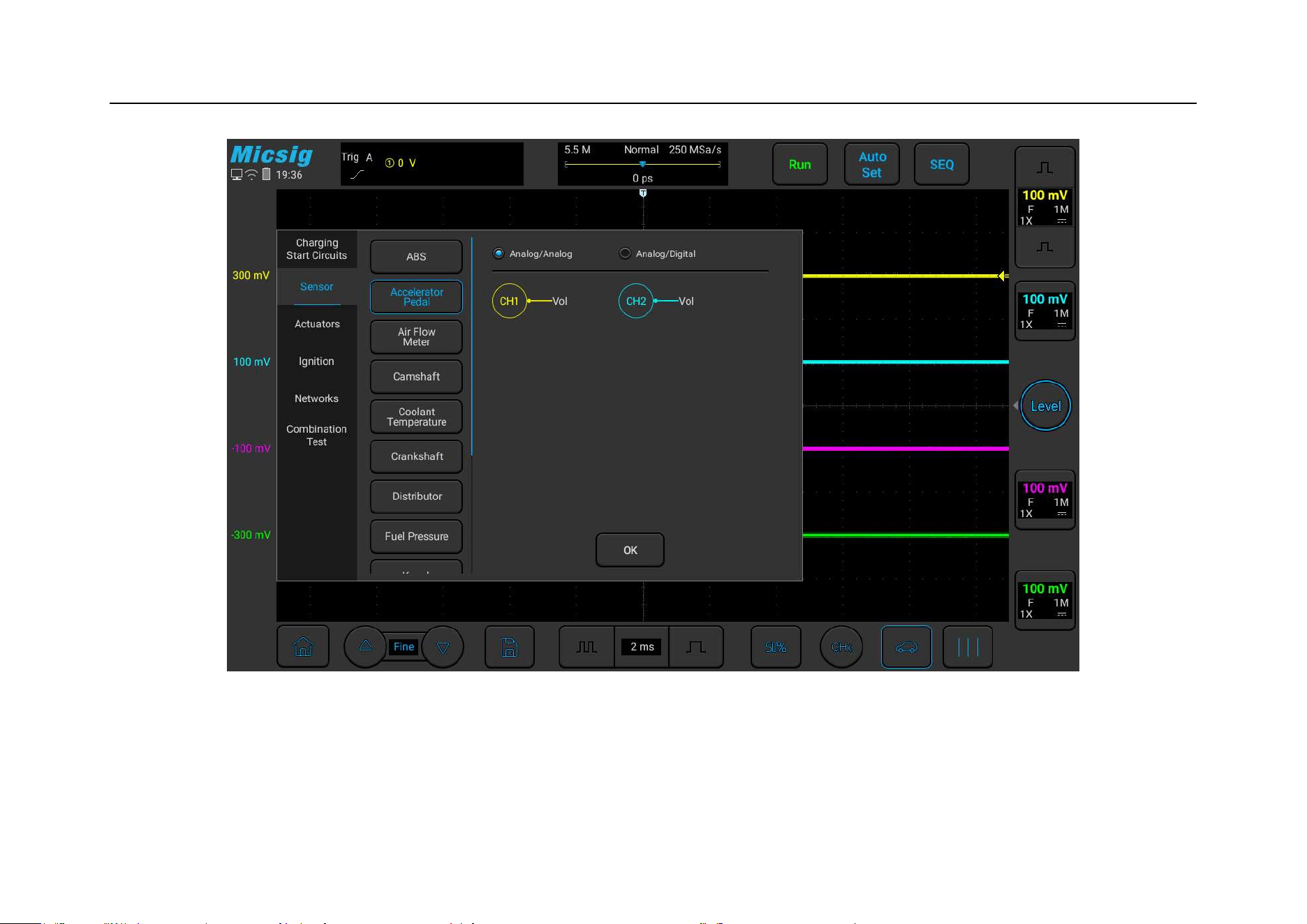
Chapter 3 Automotive Test
57
Figure 3-11 Accelerator Pedal
The following picture is the actual measurement diagram of the accelerator pedal sensor of a certain model:
58
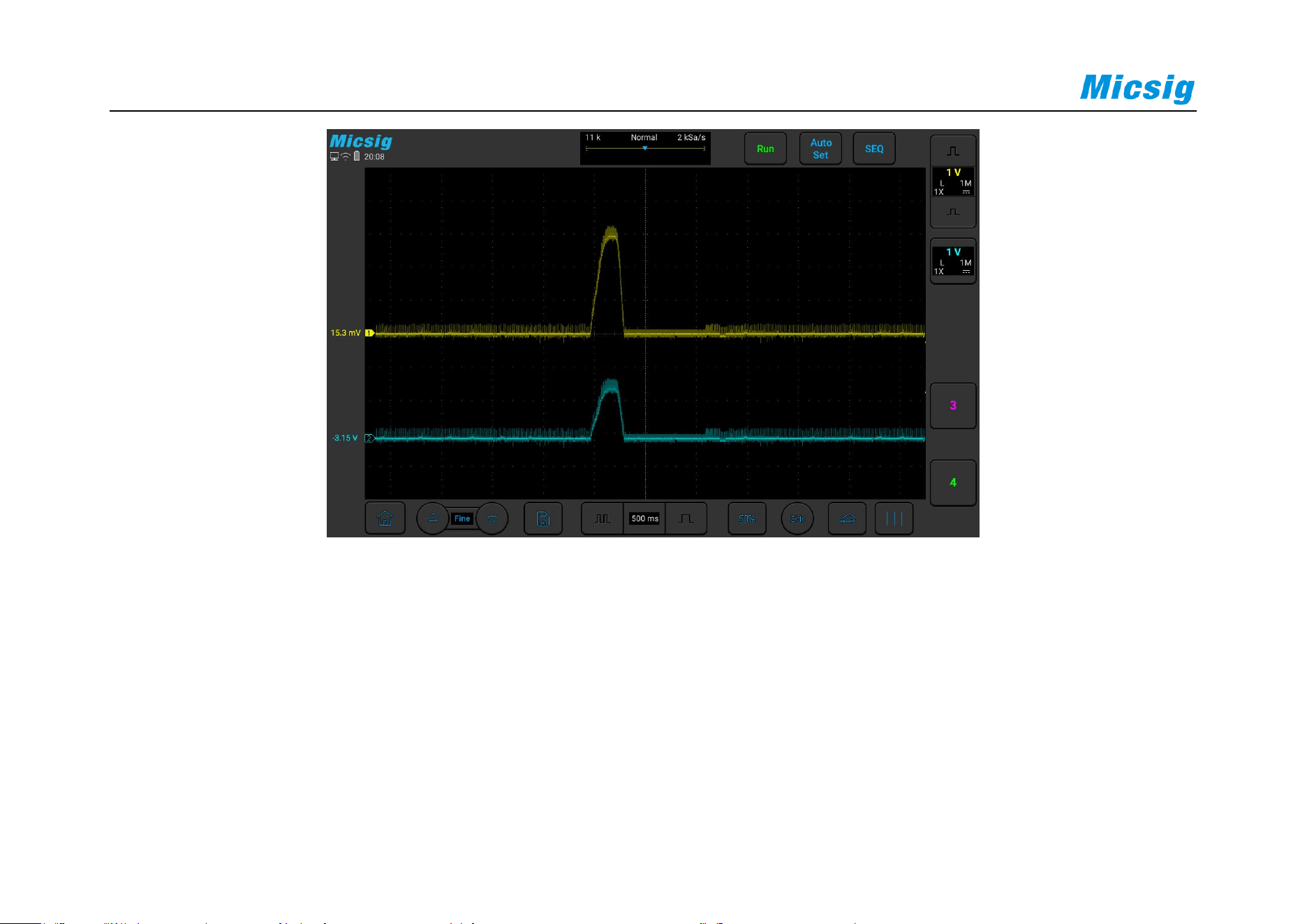
3.2.3
Air Flow Meter
Air flow meters generally have vane type, hot wire type, digital type, etc.; among them: vane type and hot wire type
are both analog output, and the output voltage is proportional to the air flow, generally 0.5V~4.5V, but the non-
linear ratio, It needs to be corrected in the ECM; the general output voltage is about 1V at idling speed, and the

Chapter 3 Automotive Test
59
voltage rises rapidly during acceleration, reaching a voltage of 4V~4.5V. After stopping the acceleration, it will
return to the idling voltage; the output shows 0V or 5V is not normal.
The digital type has a digital circuit inside the sensor. The output signal is a square wave. The frequency is used to
represent the air flow. A higher frequency means a higher air intake. Use a BNC to banana cable and connect one
end to channel 1 of the oscilloscope. The black plug on the other end is grounded, and the red connector is
connected to the signal wire of the air flow sensor with a needle. Start the vehicle, quickly depress the accelerator
pedal and release it to test, you can view the waveform.
Use the ATO oscilloscope to test the throttle air flowmeter sensor (the air flowmeter is divided into three types:
analog, digital, and hot wire, please test according to different types), the specific operation is shown in Figure 3-
12:
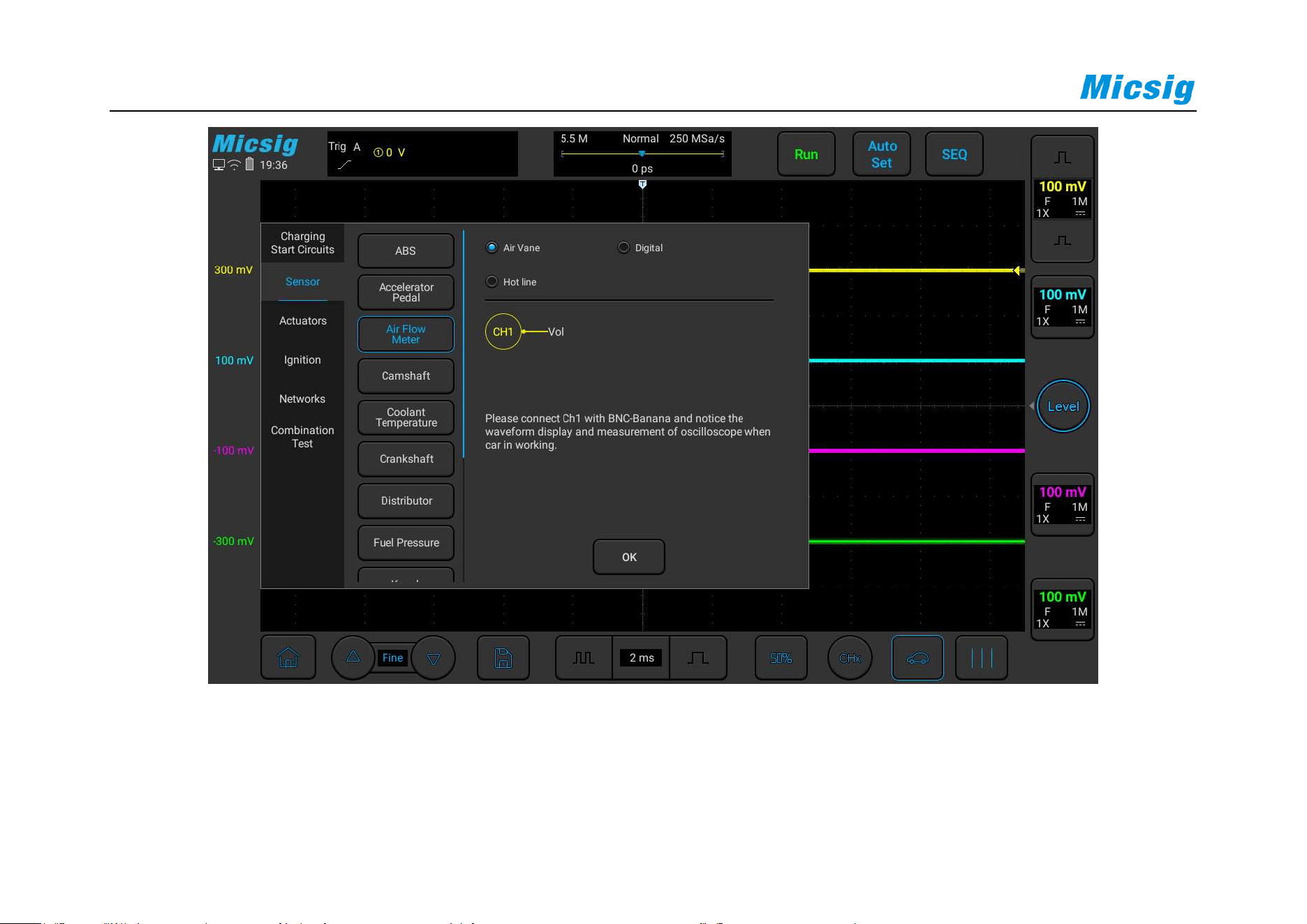
60
Figure 3-12 Air flow meter

Chapter 3 Automotive Test
61
3.2.4 Camshaft
The camshaft sensor is generally used for timing, and is often tested in conjunction with the crankshaft sensor to
determine the timing of the vehicle. There are one or two camshaft sensors in the common car models, and the use
of four is relatively small. Common camshaft sensors are Hall type/induction type/AC excitation type;
Hall sensor output is square wave, high voltage can be 5V or 12V; generally 3-wire, power, signal, ground;
inductive sensor output is a sine wave signal or square wave signal, generally 2-wire; AC excitation The output of
the type sensor is multiple sine waves (there is a missing piece at the end of the camshaft, so that the signal
changes, and the position of the No. 1 cylinder is judged at the missing place), generally 2-wire.
Use a BNC to banana cable, connect one end to channel 1 of the oscilloscope, the other end of the black plug is
grounded, and the red connector uses a needle to connect the signal line of the camshaft sensor.
Shown in Figure 3-13:
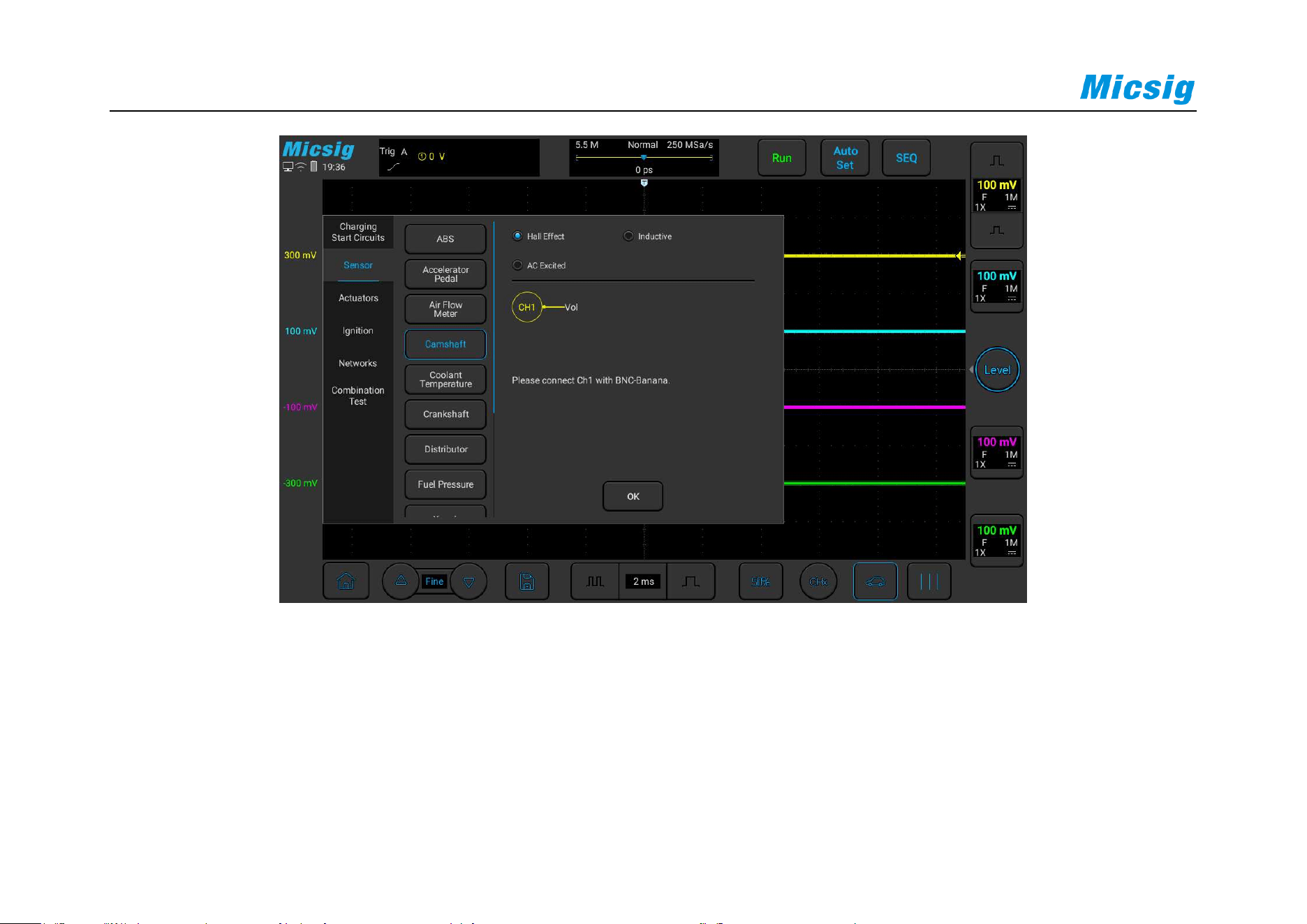
62
Figure 3-13 Camshaft
The following figure is the actual measurement diagram of the camshaft position sensor (Hall type) of a certain
model:
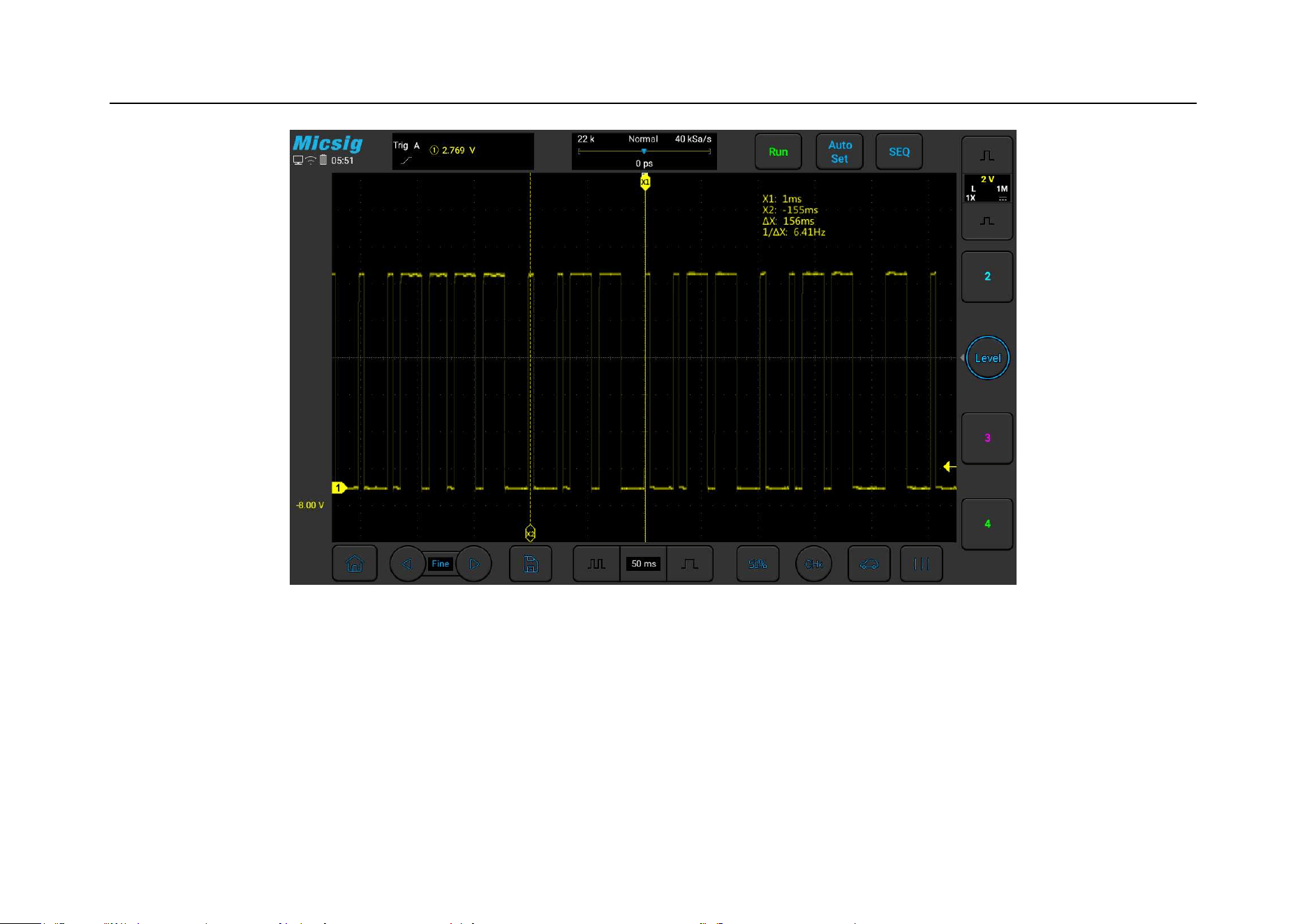
Chapter 3 Automotive Test
63
Figure 3-14 Camshaft position sensor (Hall type)
3.2.5
Coolant Temperature
The coolant temperature sensor is usually called a water temperature sensor. Generally, it contains a thermistor. As
the temperature increases, the resistance becomes smaller, which causes the output voltage to change, and the water

64
temperature changes slowly, so the voltage also changes slowly. Different models have different performances, and
the output voltage can increase with the water temperature, it can also decrease with the water temperature.
However, there is a special sensor called the Vauxhaus sensor. The output voltage of this sensor is 3-4V when the
vehicle is cold. As the vehicle starts, the temperature rises and the voltage gradually decreases. It is generally 1V
during normal operation, but as the vehicle temperature rises, when the vehicle temperature reaches 40-50 degrees,
the ECM will switch the voltage to make the sensor voltage rise rapidly to 3-4V, so as to achieve more accurate
voltage output at high temperatures.
Use a BNC to banana cable, one end is connected to channel 1 of the oscilloscope, the other end is grounded with
the black plug, and the red connector is connected to the signal wire of the coolant sensor (the ground wire of the
coolant) with a needle probe.
Use ATO oscilloscope to test the coolant temperature sensor, the specific operation is shown in Figure 3-15:
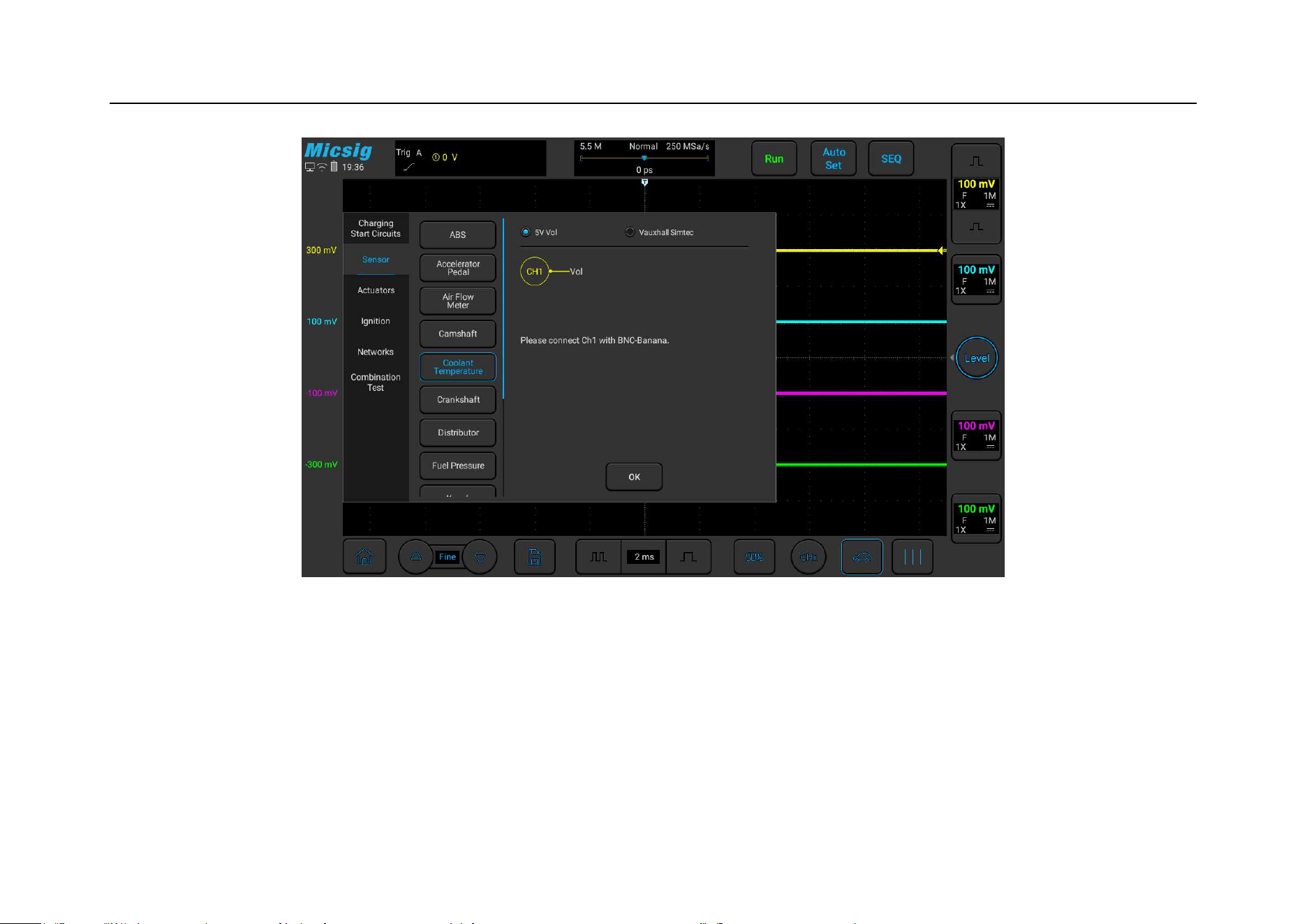
Chapter 3 Automotive Test
65
Figure 3-15 Coolant Temperature
3.2.6
Crankshaft
The crankshaft sensor is installed in many places, which can be near the front pulley or on the rear flywheel. The
ECM judges the precise position of the engine based on its output signal. Usually there are induction type and Hall

66
type: the induction type output is usually a sine wave, there are missing teeth on the disk, and the sine wave will be
missing in the missing teeth; this kind of sensor is generally 2-wire; the Hall type output is usually a square wave .
Generally 3-wire, power, signal, and ground. Use a BNC to banana cable, one end is connected to channel 1 of the
oscilloscope, the other end is grounded with the black plug, and the red connector is connected to the signal line of
the camshaft sensor with a needle.
Use the ATO oscilloscope to test the crankshaft position sensor, the specific operation is shown in Figure 3-16:

Chapter 3 Automotive Test
67
Figure 3-16 Crankshaft position sensor
The figure below is the actual measurement of the crankshaft position sensor (inductive) of a certain model:
68
3.2.7 Distributor
Distributor appears on models with high-voltage cables, and distribute the generated high voltages to spark plugs in
sequence. Distributors generally have Hall type and induction type. Hall type is generally 3-wire, voltage, signal,
and ground. The output is square wave. Inductive type is generally 2-wire. The output is sensing signal; use BNC to
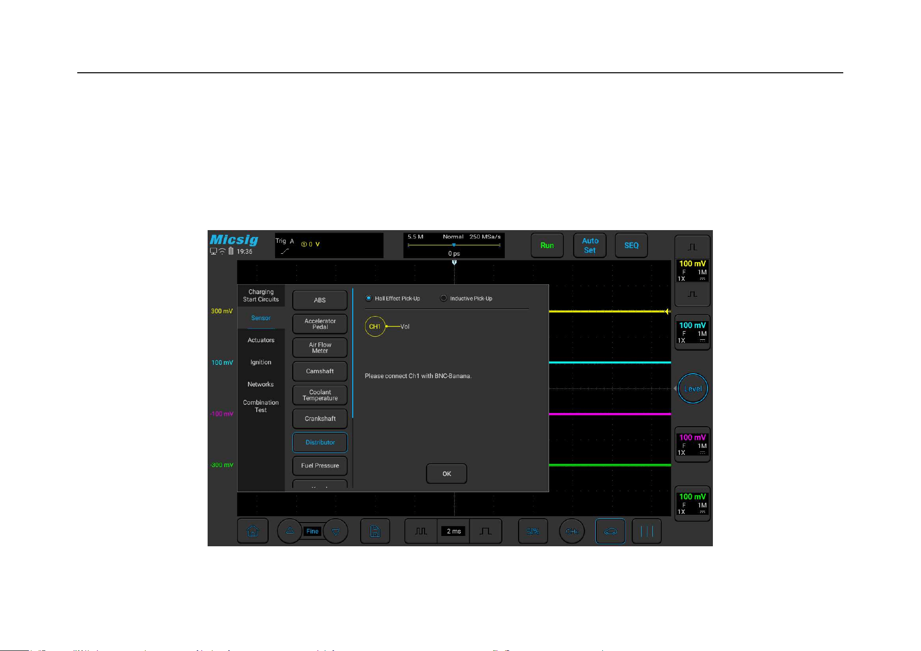
Chapter 3 Automotive Test
69
banana cable, one end is connected to channel 1 of the oscilloscope, and the other end is black The plug is
grounded, and the red connector is connected to the signal line of the distributor with a needle.
Use the ATO oscilloscope to test the distributor sensor (divided into two types: Hall effect and induction). The
specific operation is shown in Figure 3-17:
Figure 3-17 Distributor

70
3.2.8 Fuel pressure
Fuel pressure signals generally appear on high-pressure fuel rails or sensors or common rail diesel vehicles, and the
pressure is relatively high. Generally, the fuel pressure is proportional to the output voltage, and the voltage
increases with the angle of the accelerator pedal (no-load and full-load will affect the voltage rise time).
Use a BNC to banana cable, connect one end to channel 1 of the oscilloscope, the other end of the black plug is
grounded, and the red connector uses a needle to connect the signal line of fuel pressure.
Use ATO oscilloscope to test the fuel pressure sensor, the specific operation is shown in Figure 3-18:
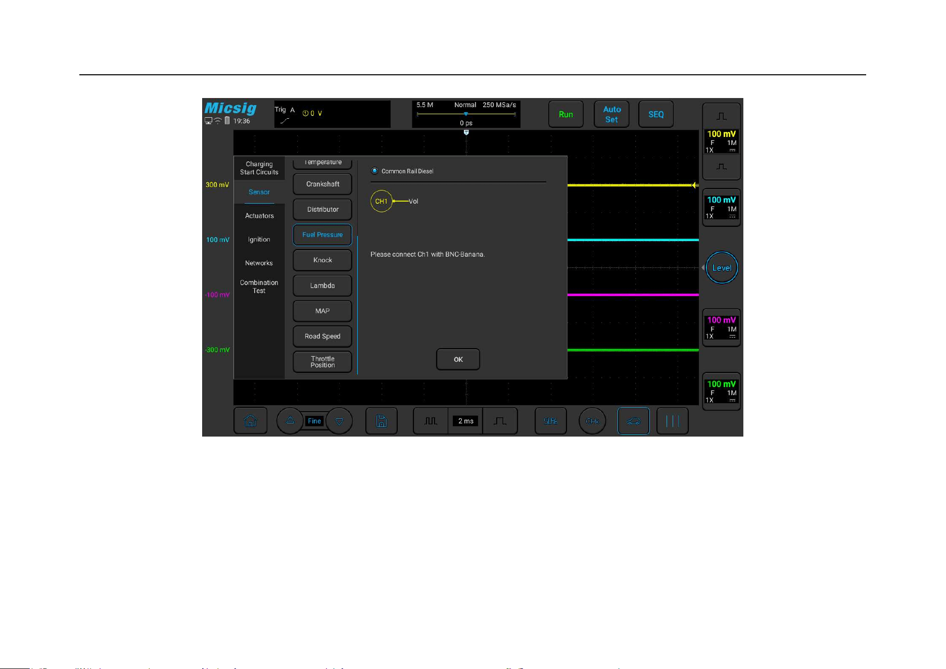
Chapter 3 Automotive Test
71
Figure 3-18 Fuel Pressure Sensor Test

72
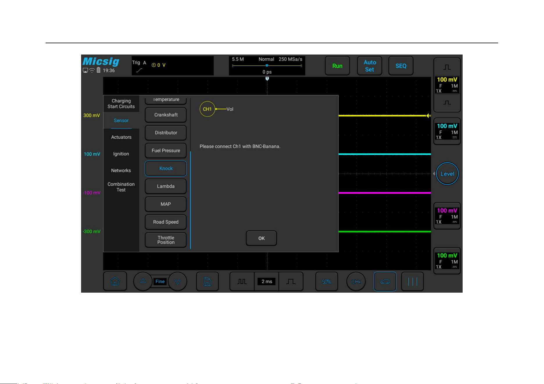
3.2.9 Knock
The knock sensor is a passive device, generally 2-wire, signal and ground, no external power supply is required,
and a signal will be generated when it is subjected to vibration. It can also be removed for testing. The signal can be
generated by tapping, and the signal amplitude generally does not exceed 5V; if the sensor is removed and then
reinstalled, please be careful not to cause excessive torque to avoid damage to the sensor.
There may be several reasons for knocking: the ignition angle is too advanced, too much carbon deposits in the
combustion chamber, the engine temperature is too high, the air-fuel ratio is too lean, the fuel is not clean enough,
and the fuel octane number is too low.
Use a BNC to banana cable, connect one end to channel 1 of the oscilloscope, the other end of the black plug is
grounded, and the red connector is connected to the signal line of the knock sensor with a needle.
Use ATO oscilloscope to test the knock sensor, the specific operation is shown in Figure 3-19:
Chapter 3 Automotive Test
73
Figure 3-19 Knock Sensor test
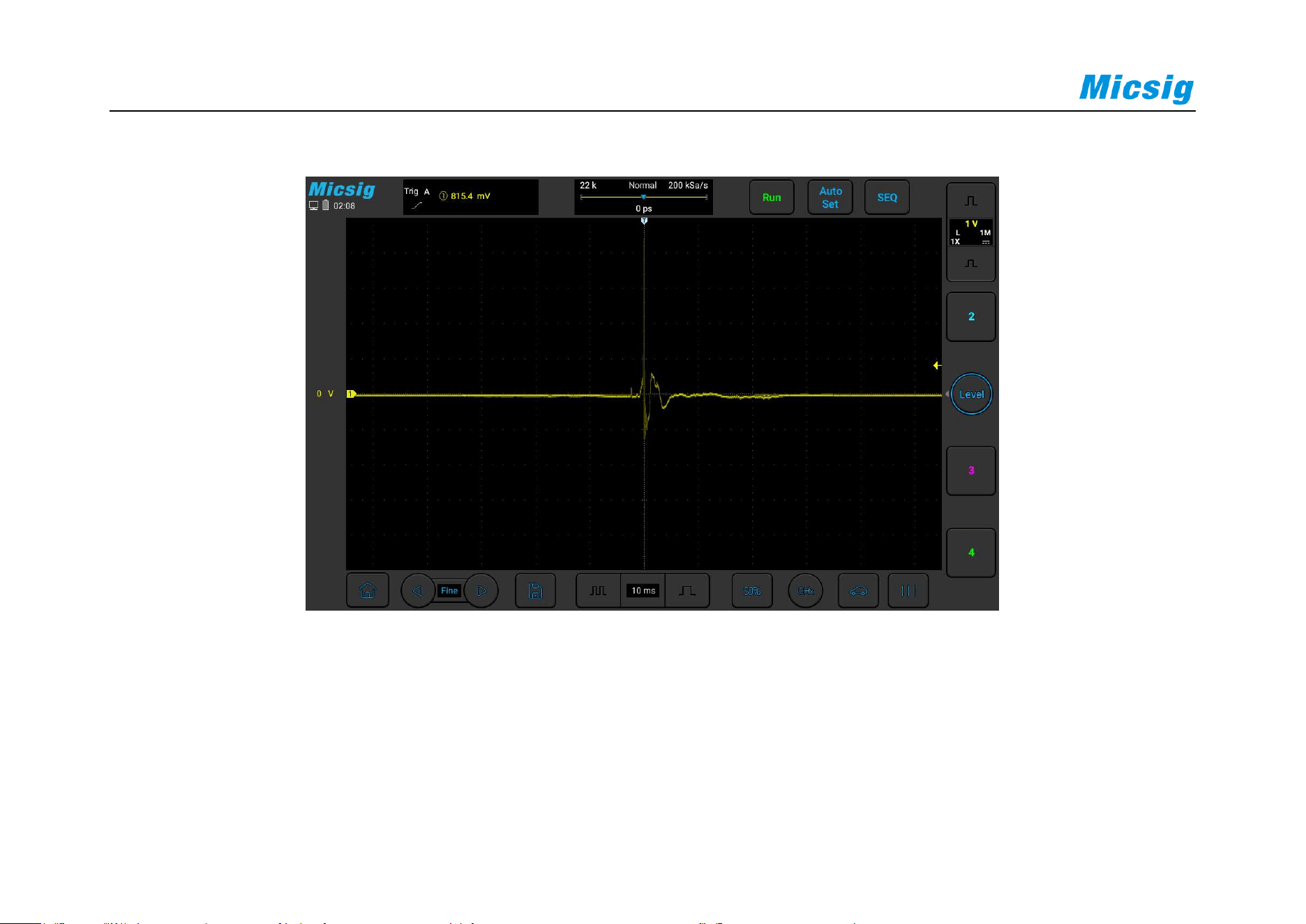
74
The following picture is the actual measurement diagram of the knock sensor of a certain model:
3.2.10
Lambda
The Lambda, or Oxygen Sensor is generally installed on the exhaust pipe, before the catalytic converter. It is a
feedback sensor used to sense the oxygen content in the exhaust gas, so that the ECM can judge the combustion
situation in the combustion chamber and adjust the fuel supply of the engine.

Chapter 3 Automotive Test
75
There are several types of oxygen sensors: titanium oxygen, zirconium oxygen, and front & rear dual oxygen
sensors; the signal switching frequency is about 1 Hz, and it can only work when the temperature is normal. The
voltage is high when the mixture is thick, and the voltage is low when the mixture is thin.
Use a BNC to banana cable, one end is connected to channel 1 of the oscilloscope, the other end is grounded with
the black plug, and the red connector is connected to the signal line (pre-oxygen) of the oxygen sensor with a
needle. Use a BNC to banana cable, connect one end to channel 2 of the oscilloscope, ground the black plug on the
other end, and use a needle to connect the red connector to the signal line of the oxygen sensor (rear oxygen, if
there is no rear oxygen sensor, no test is required). If you want to measure current, connect the BNC end of the
current clamp to channel 3 of the oscilloscope, and clamp the clamp on the heating wire.
Use ATO oscilloscope to test the oxygen sensor, the specific operation is shown in Figure 3-20:
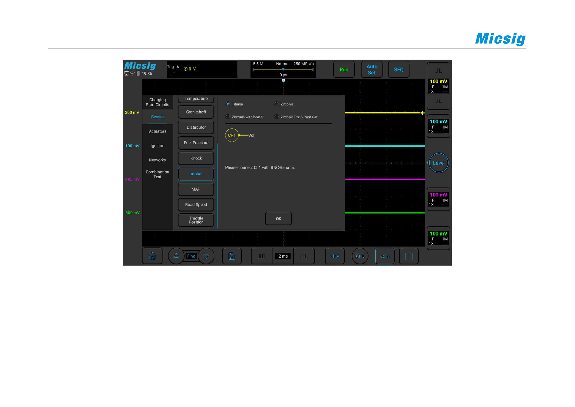
76
Figure 3-20 Lambda (oxygen sensor) test
The following picture is the actual measurement diagram of a certain model of oxygen sensor:
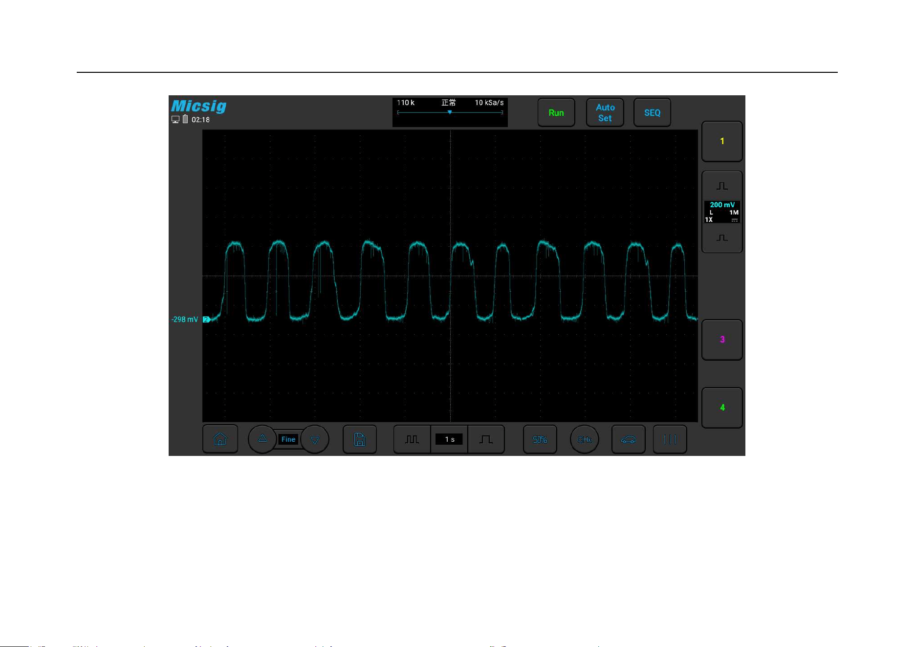
Chapter 3 Automotive Test
77
Figure 3-21 Lambda (Oxygen Sensor) diagram

78
3.2.11 MAP
The MAP, or Intake Pressure sensor is used to sense the pressure of the intake manifold and send it to the ECM to
determine the fuel supply, vacuum (or light load), and ignition timing advance angle. There are two kinds of analog
and digital, usually there are 3 wires, power, signal, ground, or together with other devices.
For the analog signal of a gasoline engine, when the throttle is closed or the engine is turned off, the output voltage
is 0, and the output is generally about 1V at idling speed (it may be slightly higher or lower). After quickly
depressing the accelerator, the throttle opens and the voltage rises rapidly. Achieve above 4.5V.
For the analog signal of the diesel engine, the voltage is between 1.5-2.0V at idling speed. After stepping on the
accelerator, the voltage can be seen to rise, which can reach 4.0V.
Use ATO oscilloscope to test the intake pressure sensor, the specific operation is shown in Figure 3-22 below:
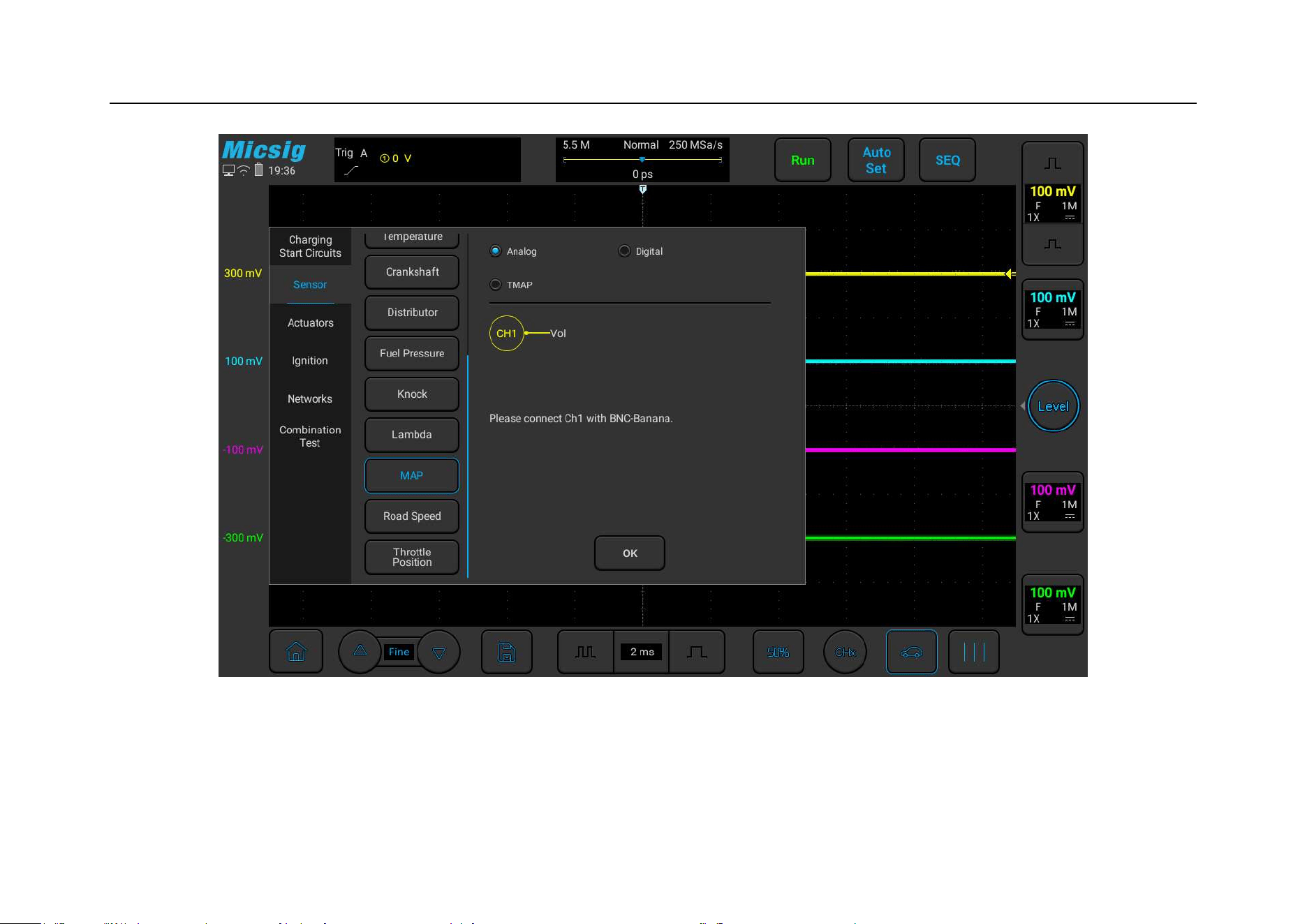
Chapter 3 Automotive Test
79
Figure 3-22 MAP (intake pressure sensor)

80
3.2.12 Road Speed
The speed sensor is generally installed on the drive output shaft of the speedometer of the gearbox or near the back
of the head of the speedometer, to provide information for the ECM and monitor power. Usually is Hall type, there
are 3 wires: power, signal, and ground, output square wave signal (some models will be analog, 2 wires, output
inductive signal, sine wave). Use a BNC to banana cable, connect one end to channel 1 of the oscilloscope, the
other end of the black plug is grounded, and the red connector is connected to the signal line of the vehicle speed
sensor with a needle. Lift the vehicle as a whole or lift the driving wheels or connect the signal to a road test, start
the vehicle, put in gear to rotate the wheels, and observe the waveform. The frequency of the square wave increases
with the increase of vehicle speed.
Use ATO oscilloscope to test the vehicle speed sensor, the specific operation is shown in Figure 3-23:
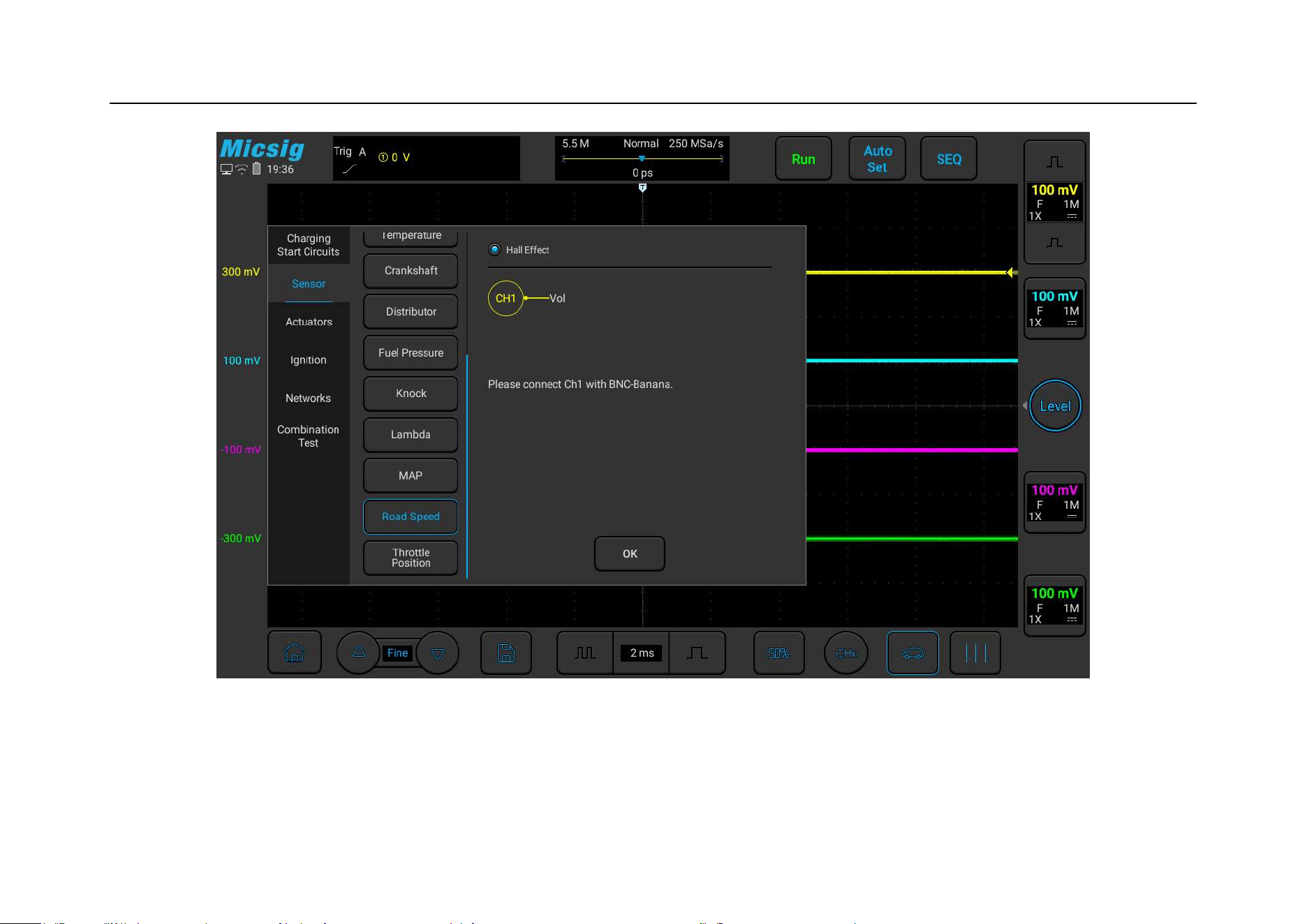
Chapter 3 Automotive Test
81
Figure 3-23 Vehicle speed sensor test

82
3.2.13 Throttle Position
The throttle position sensor is installed on the drive shaft of the throttle butterfly plate to sense the opening of the
throttle and provide a basis for ECM to judge the intake. There are analog output and throttle switch output.
Use a BNC to banana cable, connect one end to channel 1 of the oscilloscope, the other end of the black plug is
grounded, and the red connector uses a needle to connect the signal line of the throttle position sensor or the throttle
switch signal 1.
Use a BNC to banana cable, connect one end to channel 2 of the oscilloscope, the other end of the black plug is
grounded, and the red connector uses a needle to connect the signal line of the throttle position sensor, or the
throttle switch signal 2. (if it is a throttle switch, you need to connect this test lead).
Use ATO oscilloscope to test the vehicle speed sensor, the specific operation is shown in Figure 3-24:
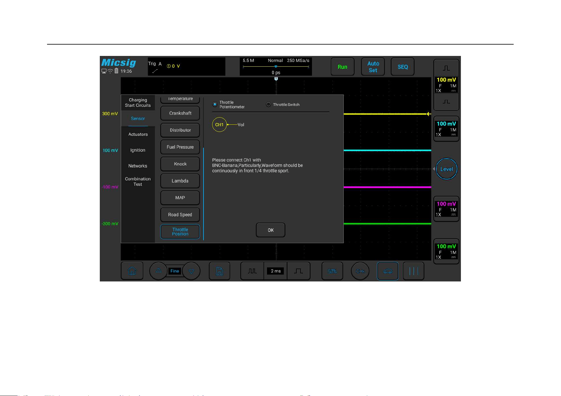
Chapter 3 Automotive Test
83
Figure 3-24 Throttle Position Sensor test
The following figure is the actual measurement diagram of the throttle position sensor of a certain model:
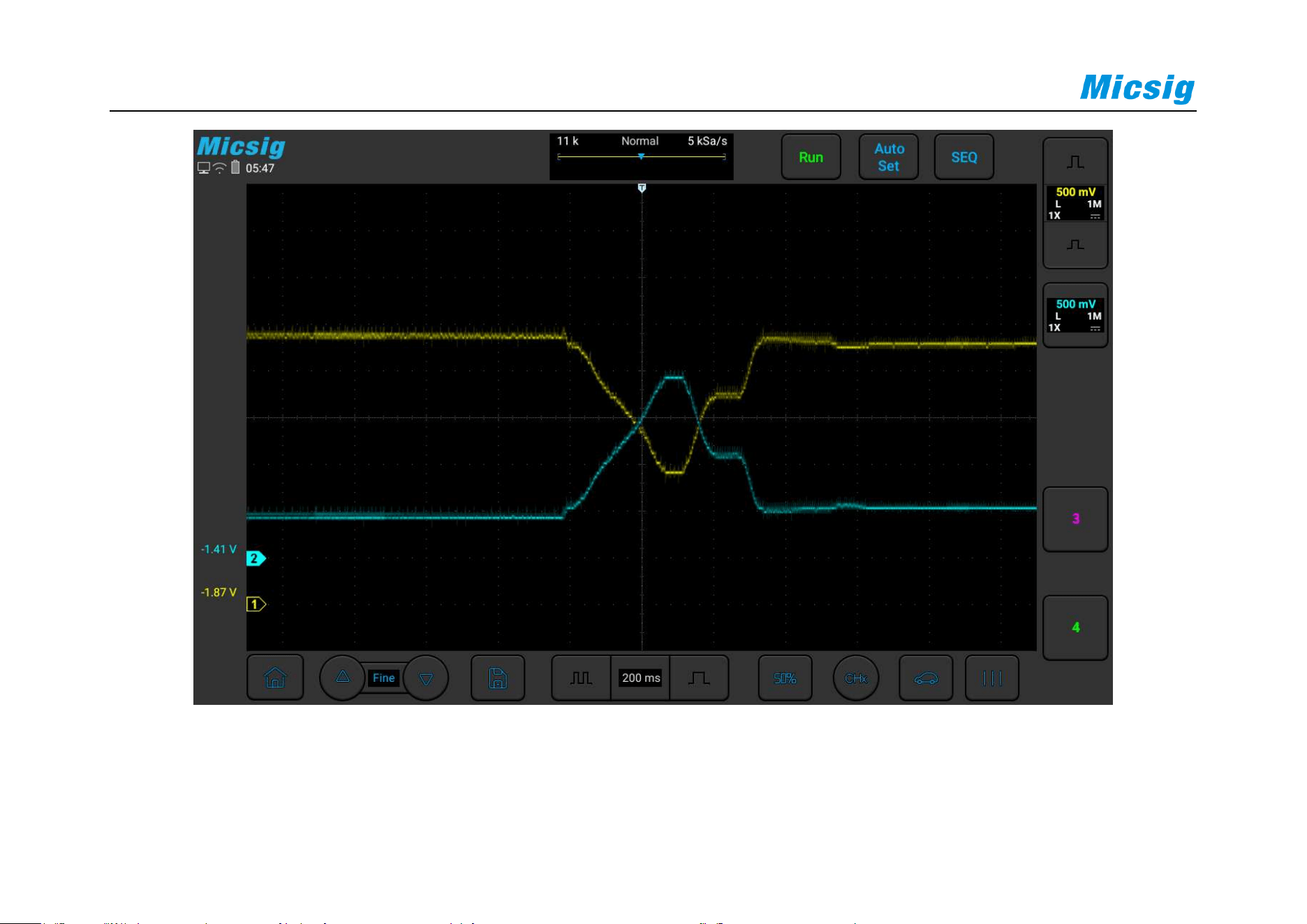
84
Figure 3-25 Throttle Position Sensor Diagram

Chapter 3 Automotive Test
85
3.3 Actuators
3.3.1
Carbon canister solenoid valve
The carbon canister is generally installed in the engine compartment and connected to the fuel tank through a pipe
to collect the vaporized oil and gas in the fuel tank, so as to prevent the oil and gas from being discharged into the
air and causing pollution. Use a BNC to banana cable, one end is connected to channel 1 of the oscilloscope, the
other end of the black plug is grounded, and the red connector is connected to the ground wire of the canister
solenoid valve with a needle tip.
Use ATO oscilloscope to test the vehicle speed sensor, the specific operation is shown in Figure 3-26:

86
Figure 3-26 Carbon canister solenoid valve test
The following figure is the actual measurement of the Carbon canister solenoid valve of a Audi A6 model in a
certain year:
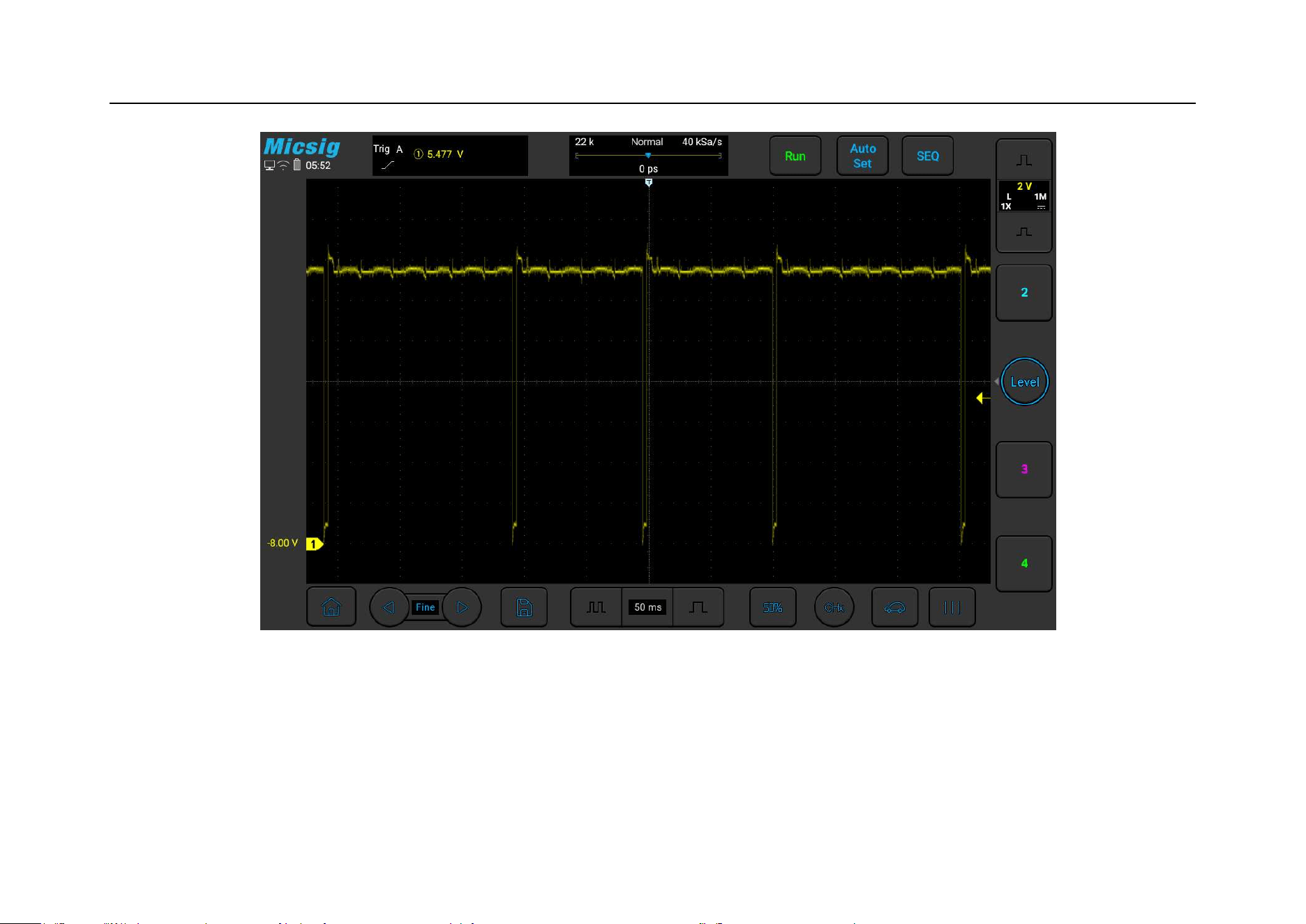
Chapter 3 Automotive Test
87
Figure 3-27 Audi A6 Carbon canister solenoid valve signal

88
3.3.2 Disel Glow Plugs
When the engine or the weather is relatively cold, it will affect the combustion of diesel fuel, so the glow plug is
required to heat the cylinder before starting. Diesel engine glow plugs generally have one for each cylinder,
connected in series, powered by a battery, and controlled by a relay to open and close.
When the ambient temperature is low or the engine temperature is relatively low, when starting the vehicle, the
glow plug will be turned on first, and after the preheating light goes out, the vehicle can be started to make the
engine idling.
Use a current clamp, connect one end to channel 1 of the oscilloscope, and clamp the other end to the power cord of
the glow plug. Pay attention to the direction of the current.
ATO oscilloscope can be used to test the diesel engine glow plug (according to the type of glow plug, there are two
types: glow plug and single glow plug).
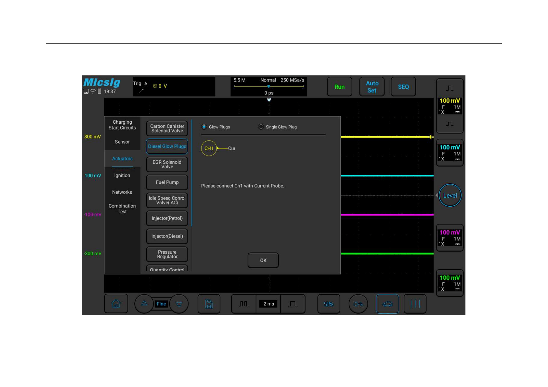
Chapter 3 Automotive Test
89
The specific operation is shown in Figure 3-28 below:
Figure 3-28 Disel Glow Plugs

90
3.3.3 EGR Solenoid Valve
The EGR solenoid valve is an abandoned recirculation solenoid valve. After opening, a part of the exhaust gas will
be sucked into the intake manifold again to reduce the combustion temperature, so as to reduce the emission of
nitrogen oxides in the exhaust gas and achieve the goal of environmental protection. Use a BNC to banana cable,
one end is connected to channel 1 of the oscilloscope, the other end is grounded with the black plug, and the red
connector is connected to the ground wire of the EGR solenoid valve with a needle.
Use ATO oscilloscope to test the EGR solenoid valve, the specific operation is shown in Figure 3-29:
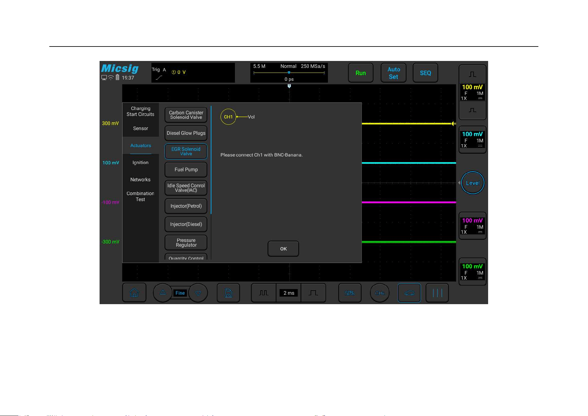
Chapter 3 Automotive Test
91
Figure 3-29 EGR solenoid valve test

92
3.3.4 Fuel Pump
The fuel in the fuel tank can be pumped and pressurized through the fuel pump, usually there are 6-8 sectors. Under
the same condition of the engine, a good fuel pump has the same and uniform current change in each sector.
Use a current clamp, connect one end to channel 1 of the oscilloscope, and clamp the other end to the power line of
the fuel pump. Pay attention to the direction of the current. (You can also use the corresponding fuse, replace it with
a extension cord and clamp on the cord of the current clamp).
Use ATO oscilloscope to test the electronic fuel pump, the specific operation is shown in Figure 3-30 below:
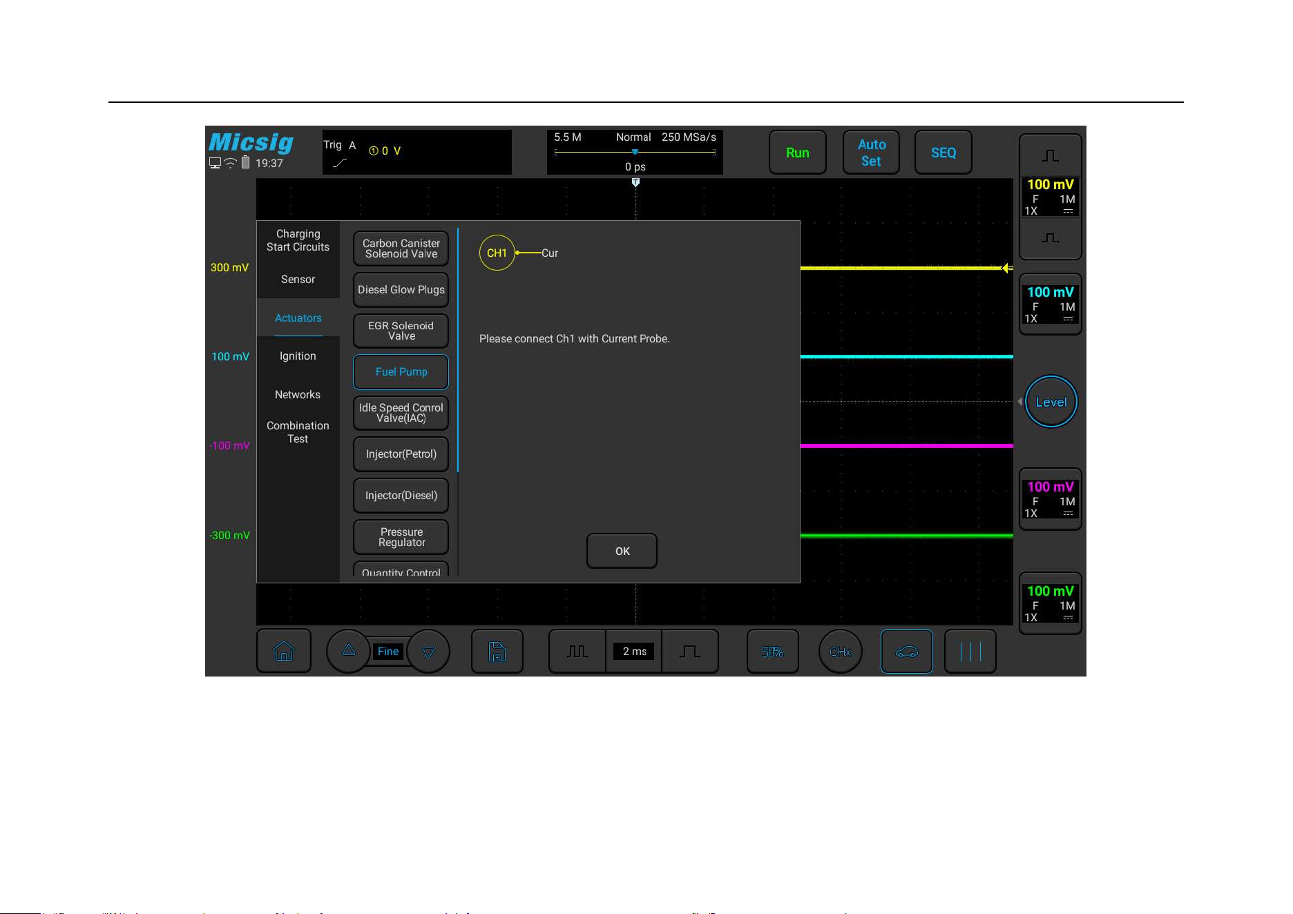
Chapter 3 Automotive Test
93
Figure 3-30 Electronic fuel pump test

94
3.3.5 Idle speed control valve
The idle speed control valve adjusts the throttle position or forms an air bypass around the engine according to the
load conditions of the engine and the engine temperature to deliver controllable airflow to the air duct to adjust the
engine idle speed. For gasoline vehicles, generally when the engine is cold started , The engine speed will rise
rapidly to about 1200 rpm. When the engine reaches the normal operating temperature, the idle speed will gradually
decrease, and finally stabilize at the preset value.
Use ATO oscilloscope to test the idle speed control valve, the specific operation is as shown in Figure 3-31:
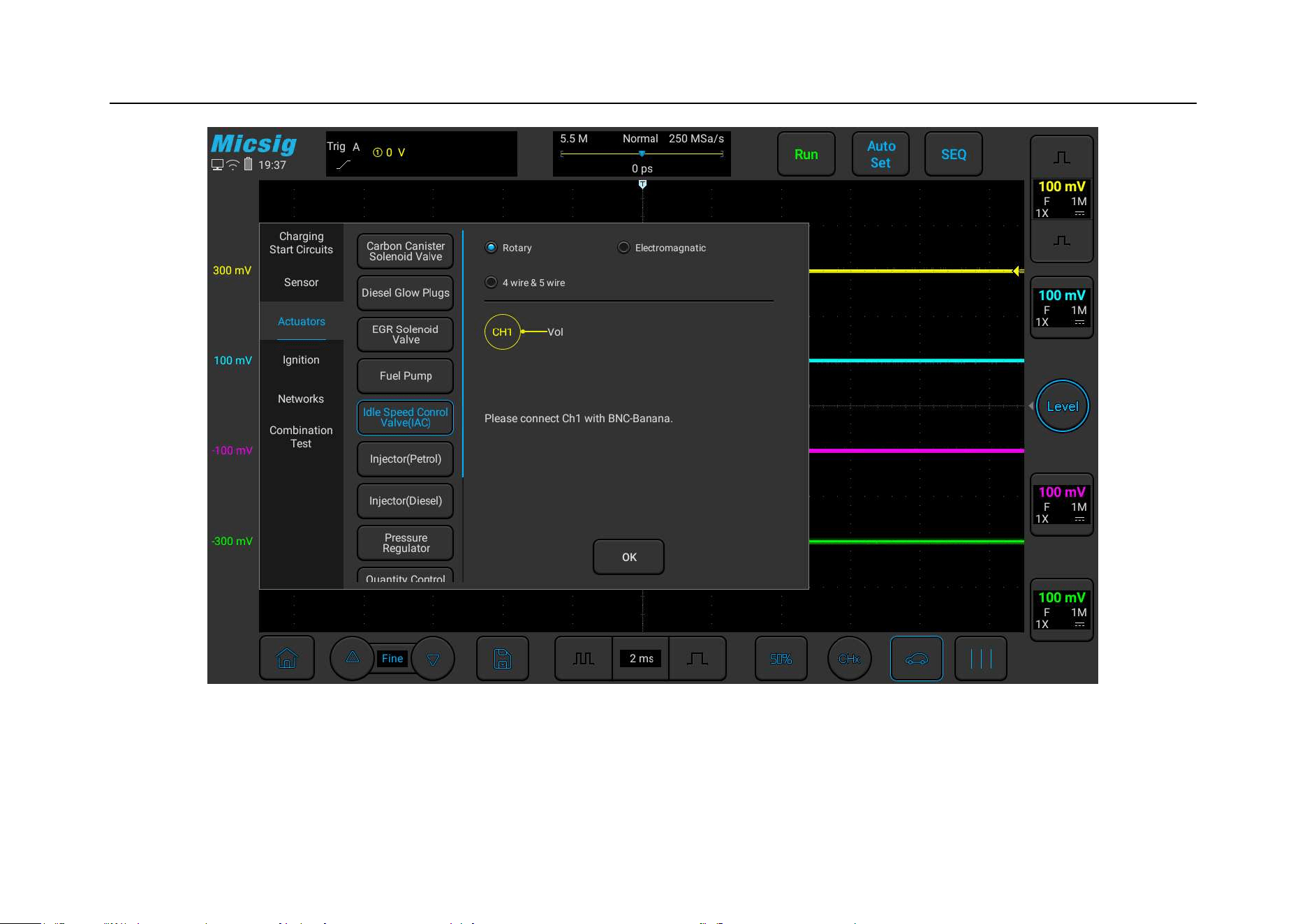
Chapter 3 Automotive Test
95
Figure 3-31 Idle speed control valve test

96
3.3.6 Injector (gasoline engine)
The fuel injector is an electromechanical device, which is supplied by a common rail fuel pipe and controlled by the
ECM to start and stop time of fuel injection. Generally, it is a 2-wire device, the power supply voltage is 12V, and
the ECM controls the grounding. Limited by cost, some vehicles are equipped with single-point fuel injectors. The
single-point fuel injection pressure is low and the airflow from intake pipe can make a mist of fuel for better
combustion.
Use ATO oscilloscope to test the fuel injector, the specific operation is shown in Figure 3-32:
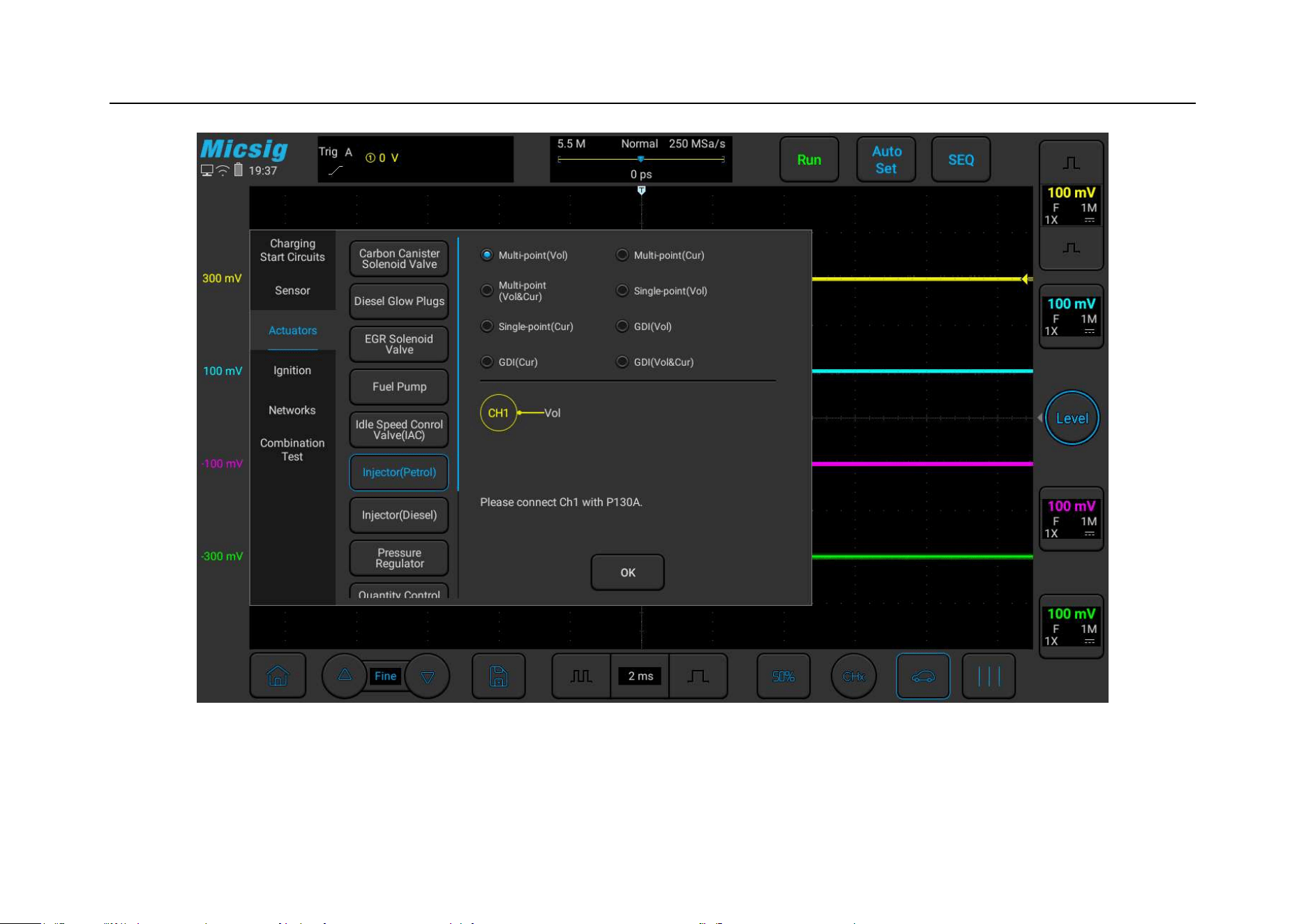
Chapter 3 Automotive Test
97
Figure 3-32 Injector (Petrol) Test

98
3.3.7 Injector (Diesel)
Most diesel engines use common rail fuel injection, fuel injection time is affected by the oil pressure. Low pressure
at low speed, injection time is longer, less injection volume; High pressure at high speed, injection time is short,
volume is large. There are mainly Bosch common rail injectors, Delphi injectors, CDi version 3 system injectors,
piezoelectric injectors, Volkswagen Audi's PD system, Volkswagen Audi's piezoelectric PD, etc. on the market.
Use ATO oscilloscope to test the fuel injector (diesel engine), the specific operation is shown in Figure 3-33:
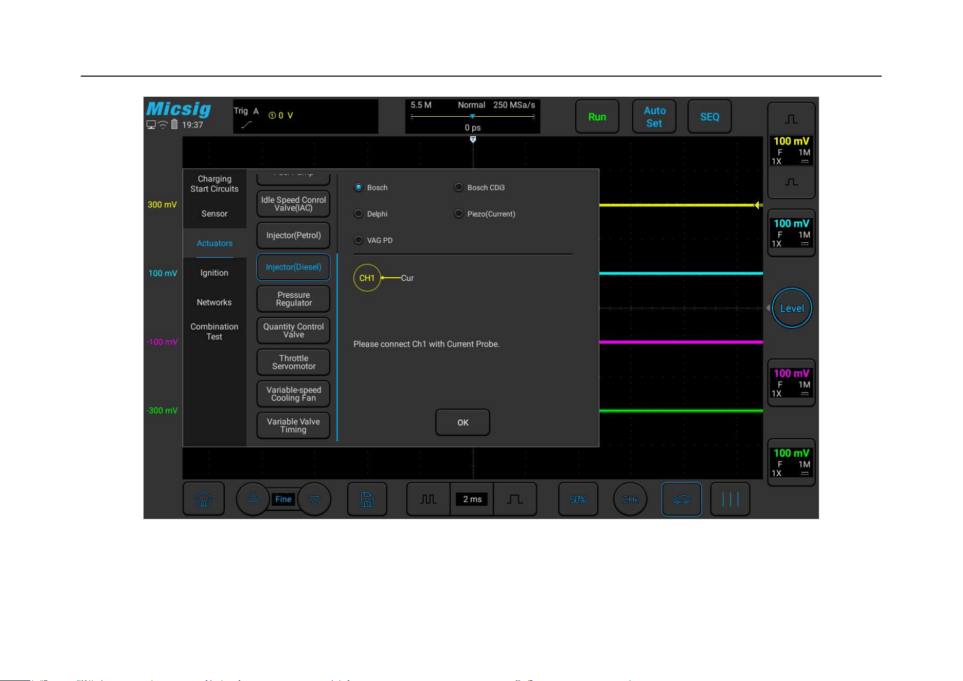
Chapter 3 Automotive Test
99
Figure 3-33 injector (diesel engine) test

100
3.3.8 Pressure regulator
The pressure regulator is a valve controlled by a square wave duty cycle. It is installed on the high-pressure fuel
pump or on the common rail pipe and controls the common rail pressure together with the flow control valve. The
pressure relief valve simply controls the amount of high-pressure oil entering the oil return system, thereby
increasing or decreasing the fuel pressure of the common rail pipe. Use a BNC to banana cable, connect one end to
channel 1 of the oscilloscope, the other end of the black plug is grounded, and the red connector is pierced into the
end of the pressure regulator signal line with a needle probe.
Use ATO oscilloscope to test the pressure regulator, the specific operation is shown in Figure 3-34:
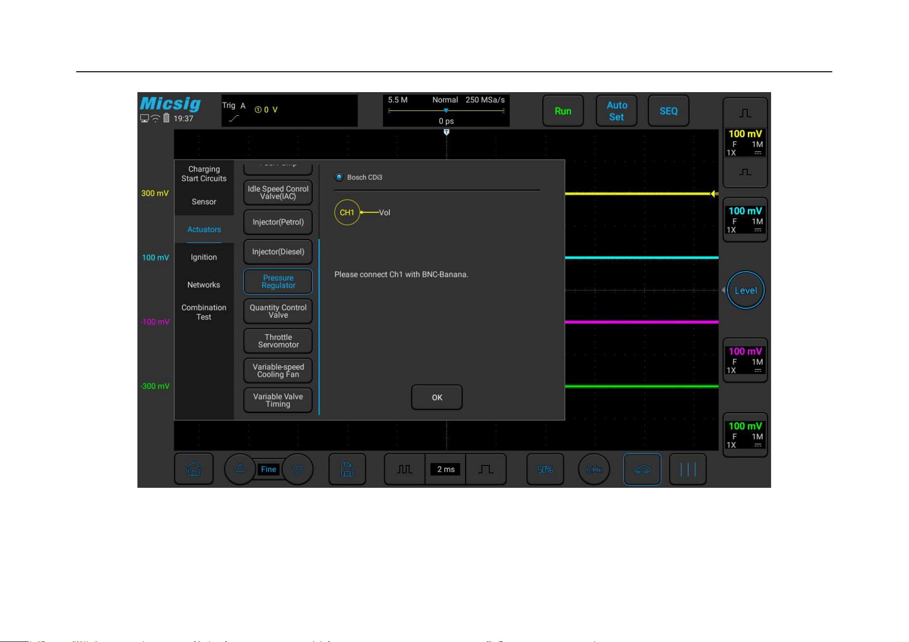
Chapter 3 Automotive Test
101
Figure 3-34 Pressure Regulator test

102
3.3.9 Quantity (Flow) control valve
The flow control valve, also known as the flow regulator and the fuel inlet metering valve, is used to measure the
flow of fuel from the low pressure or lift pump into the high-pressure fuel pump. The more fuel enters the piston
chamber of the high-pressure fuel pump, the higher the pressure, which increases the pressure in the common rail
fuel pipe; on the contrary, the lower the pressure. Generally, two wires, signal (power) and ground.
Use ATO oscilloscope to test the flow control valve, the specific operation is shown in Figure 3-35:
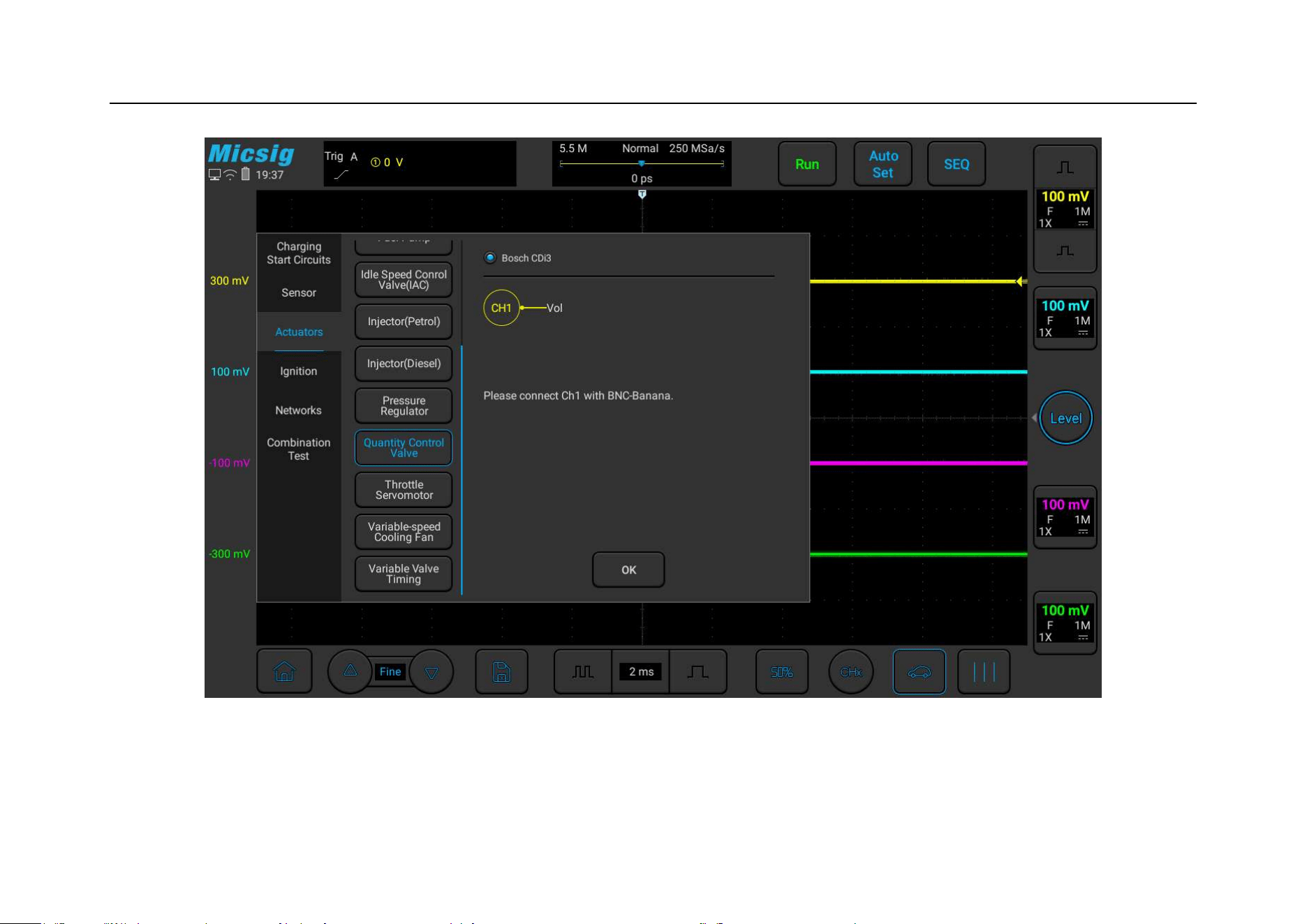
Chapter 3 Automotive Test
103
Figure 3-35 Quantity (Flow) control valve test

104
3.3.10 Throttle Servo Motor
Throttle servo motor are commonly used in electronically controlled engines, and throttle butterfly valves are
usually used. The ECM controls the throttle servo motor according to the accelerator pedal signal to realize the
throttle opening control, which is then monitored by the throttle position sensor and transmits the signal back to the
ECM to achieve closed-loop control.
Use ATO oscilloscope to test the throttle servo motor, the specific operation is shown in Figure 3-36:
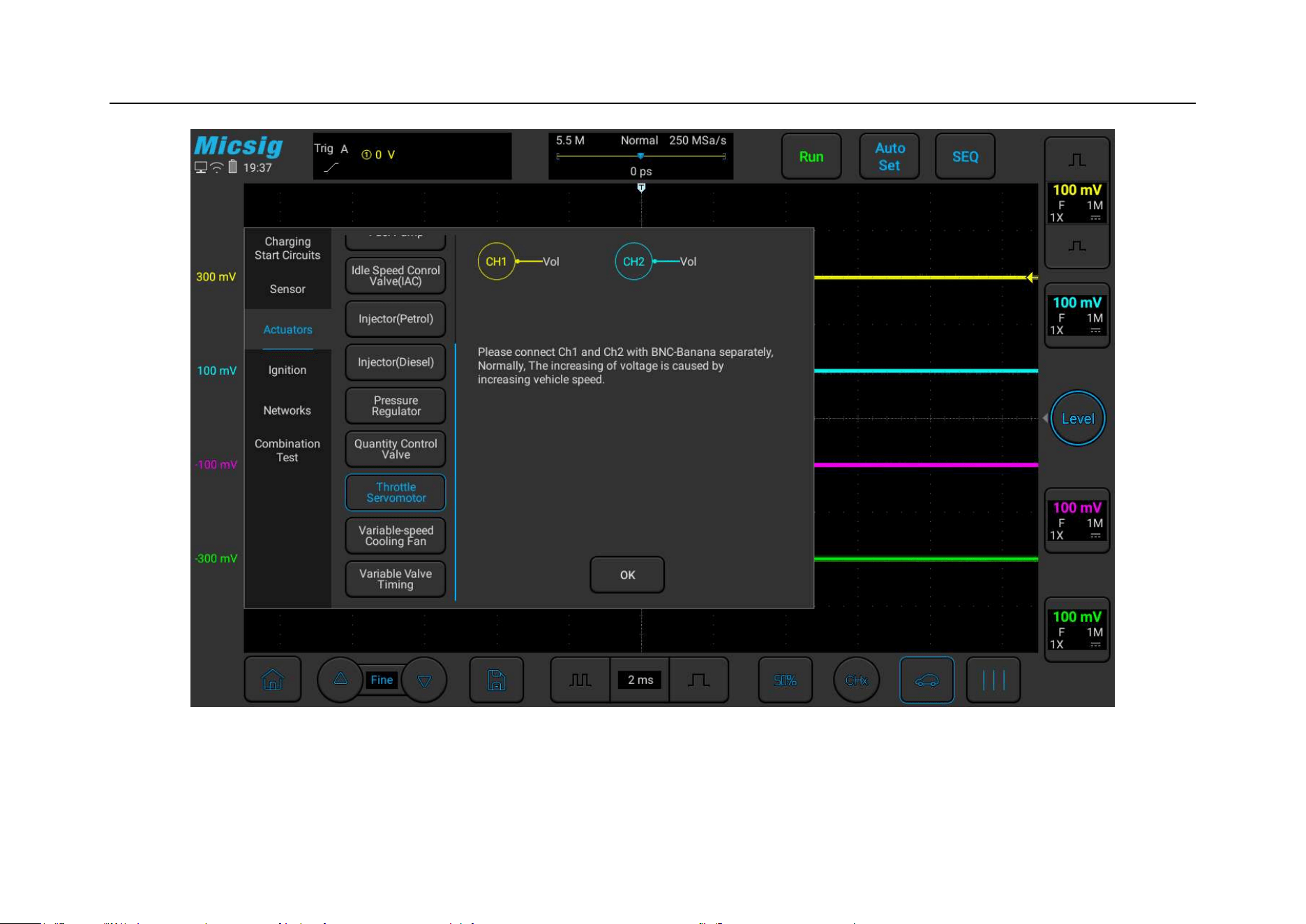
Chapter 3 Automotive Test
105
Figure 3-36 Throttle servo motor test

106
3.3.11 Variable speed cooling fan
At present, most cars' fans are variable-speed, and the speed of the fan can be adjusted according to different
working conditions and temperatures.
Use a BNC to banana cable, connect one end to channel 1 of the oscilloscope, ground the other end of the black
plug, and use a needle to pierce the red connector into the signal wire of the fan terminal; use a current clamp,
connect one end to channel 2 of the oscilloscope, and clamp the other end to it Pay attention to the direction of the
current on the fan's power cord. (If you need to test the current, connect a current clamp).
Use ATO oscilloscope to test the cooling fan, the specific operation is shown in Figure 3-37:
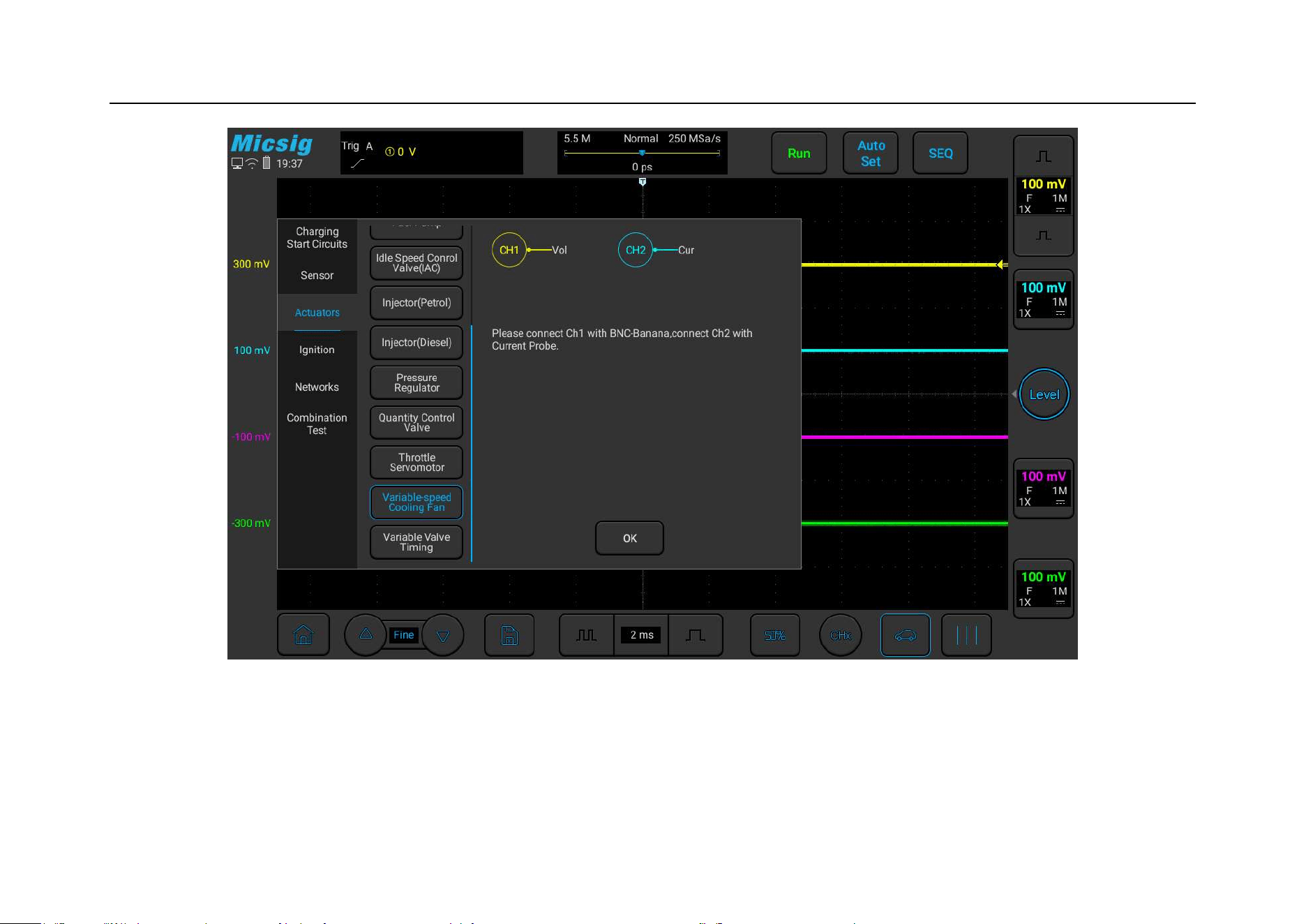
Chapter 3 Automotive Test
107
Figure 3-37 Variable-speed Cooling fan test
The following picture is the actual measurement diagram of the cooling fan of a certain model:
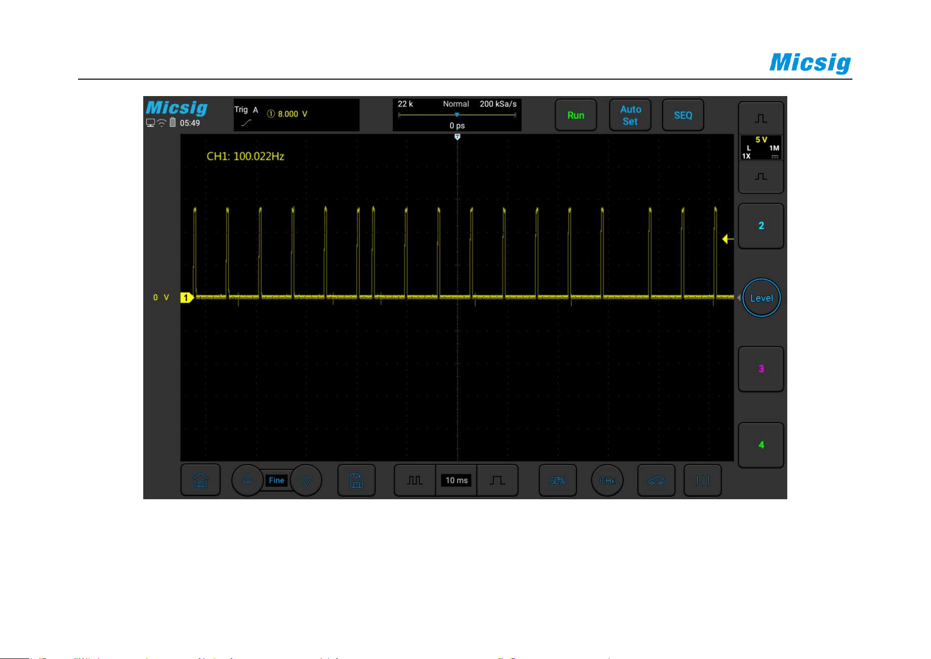
108
Figure 3-38 Cooling fan measurement diagram

Chapter 3 Automotive Test
109
3.3.12 Variable valve timing
Variable valve timing is achieved by adjusting the phase of the engine cam so that the intake air volume changes
with the change of engine speed, so as to achieve the best combustion efficiency and improve fuel economy. Use a
BNC to banana cable, connect one end to channel 1 of the oscilloscope, the other end of the black plug is grounded,
and the red connector is pierced into the variable valve timing signal line with a needle tip.
Use the ATO oscilloscope to test the variable valve timing (divided into single and double timing), the specific
operation is shown in Figure 3-39:
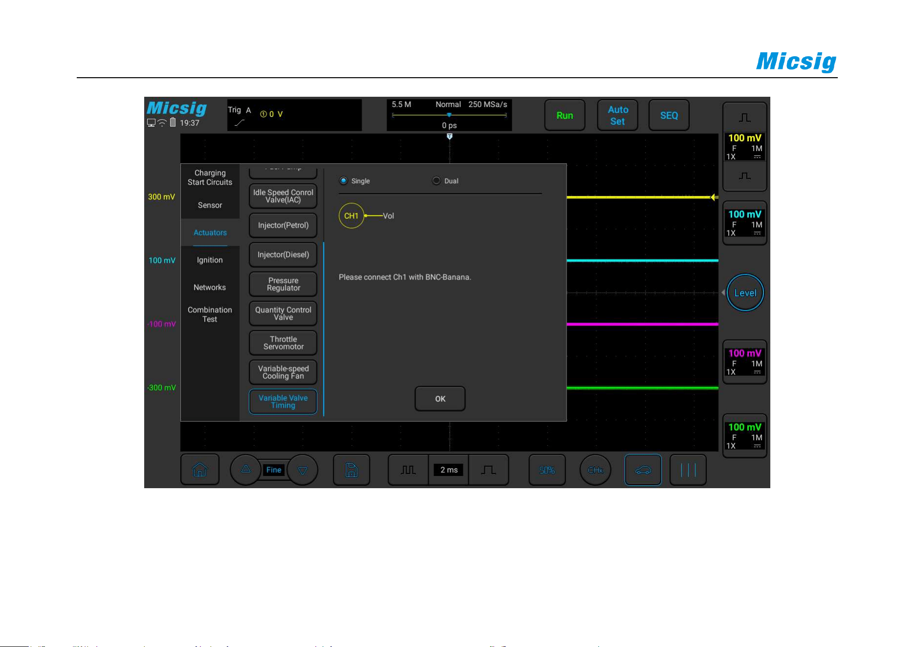
110
Figure 3-39 Variable valve timing test
The following picture is the actual measurement diagram of the Variable valve timing of a certain model:
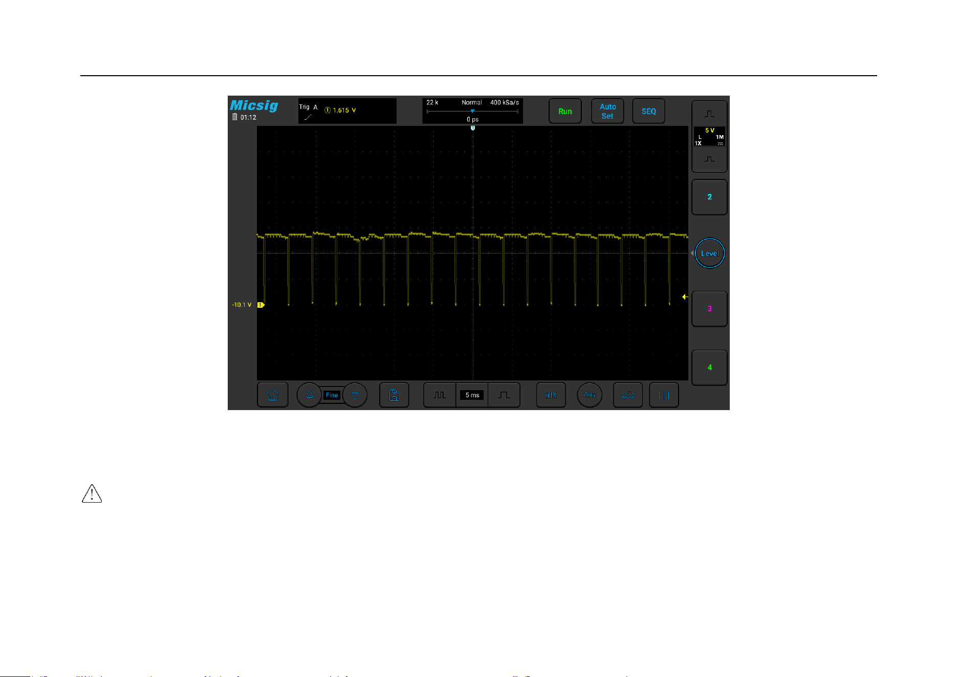
Chapter 3 Automotive Test
111
3.4 Ignition Tests
Special Attention! During the secondary ignition test, because the test voltage is about 40K volts, the secondary
ignition probe must be used for operation. It is strictly forbidden to use the ordinary probe, otherwise it is very
likely to cause personal safety injury and instrument damage.

112
3.4.1 Primary
The ignition system of a gasoline car usually consists of a primary coil, a secondary coil and a spark plug. There are
traditional ignition systems and electronic ignition systems. Currently, most car models already use electronic
ignition systems. The primary circuit has developed from the basic contact type and capacitive type to the system
with no distributor and one coil per cylinder that is commonly used today.
Use a P130A probe, connect one end to channel 1 of the oscilloscope, and connect the other end to the ground with
the black clip. Use a stinger to pierce the ground wire of the primary coil and hook the probe to the metal needle of
the stinger; use a current clamp to connect the other end to channel 2 of the oscilloscope. Clamp the other end on
the power cord of the primary coil, pay attention to the direction of the current (if you need to test the current,
connect a current clamp).
Use the ATO oscilloscope to test the primary ignition coil (the voltage, current, voltage + current, signal can be
tested separately to help users troubleshoot possible faults), the specific operation is shown in Figure 3-40:
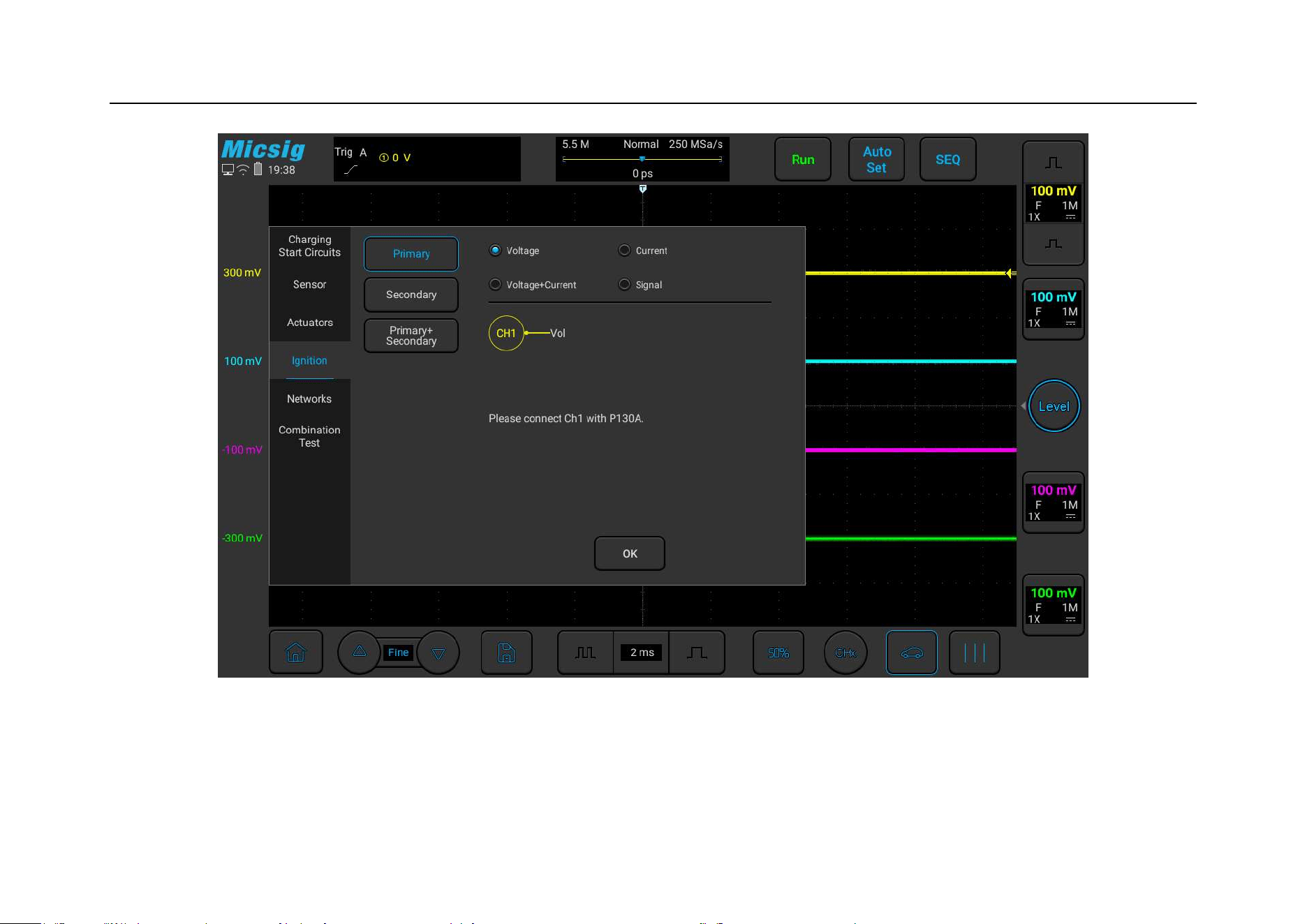
Chapter 3 Automotive Test
113
Figure 3-40 Primary ignition
The figure below is the actual measurement of the primary ignition of a certain model:
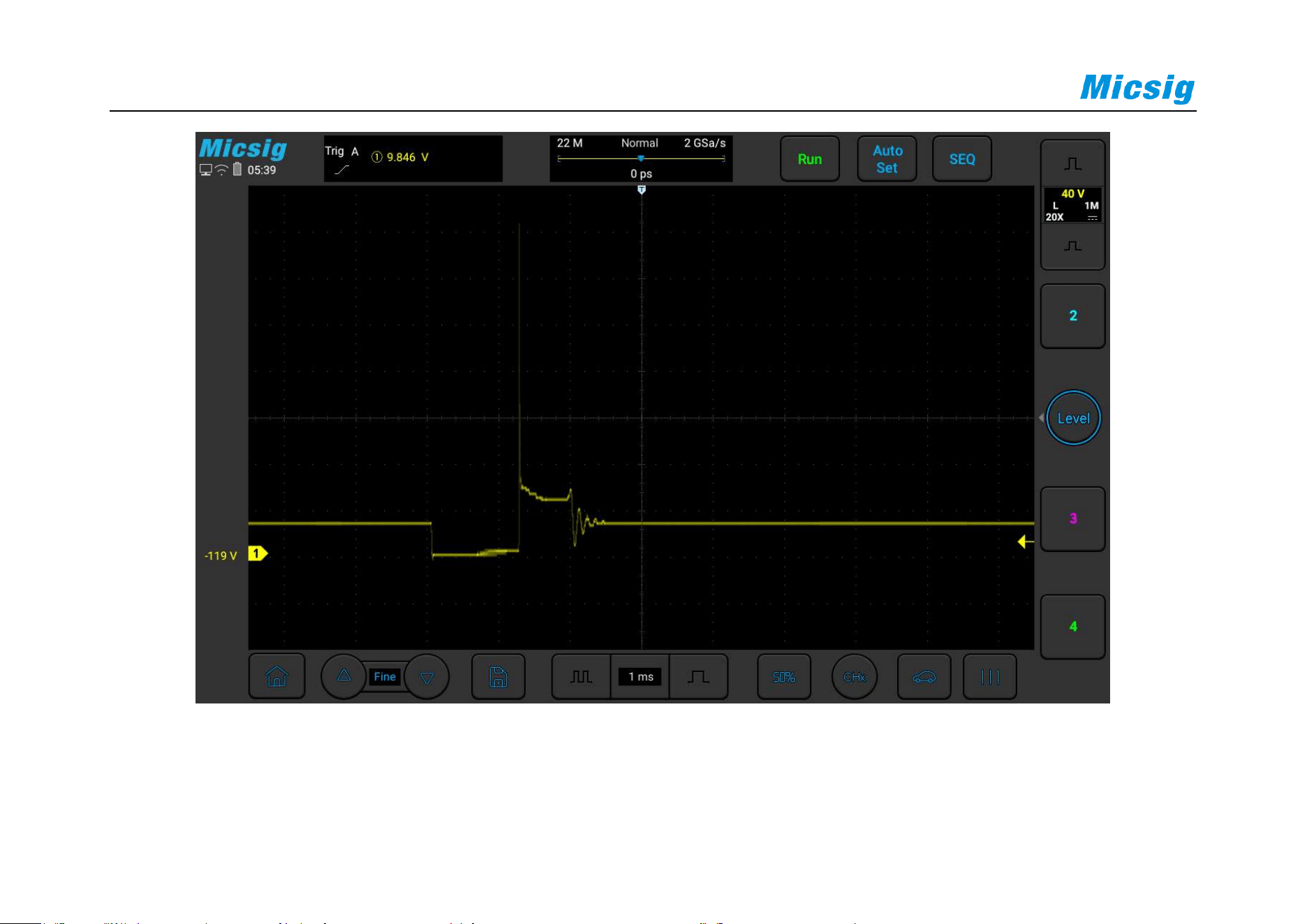
114
Figure 3-41 Primary ignition actual test

Chapter 3 Automotive Test
115
3.4.2 Secondary
The secondary coil has more coil turns than the primary coil, and can generate a high voltage of up to 40kv, which
can cause the spark plug to break down and ignite. There are several types: distributor ignition system,
distributorless ignition system/invalid spark, COP independent ignition, multi-COP integrated unit ignition.
Use the ATO oscilloscope to test the secondary ignition coil ( must use the secondary ignition probe) [the
voltage (KV), coil output voltage, and voltage (mv) can be tested separately to help users troubleshoot possible
faults]. The specific operations are as follows Figure 3-42:
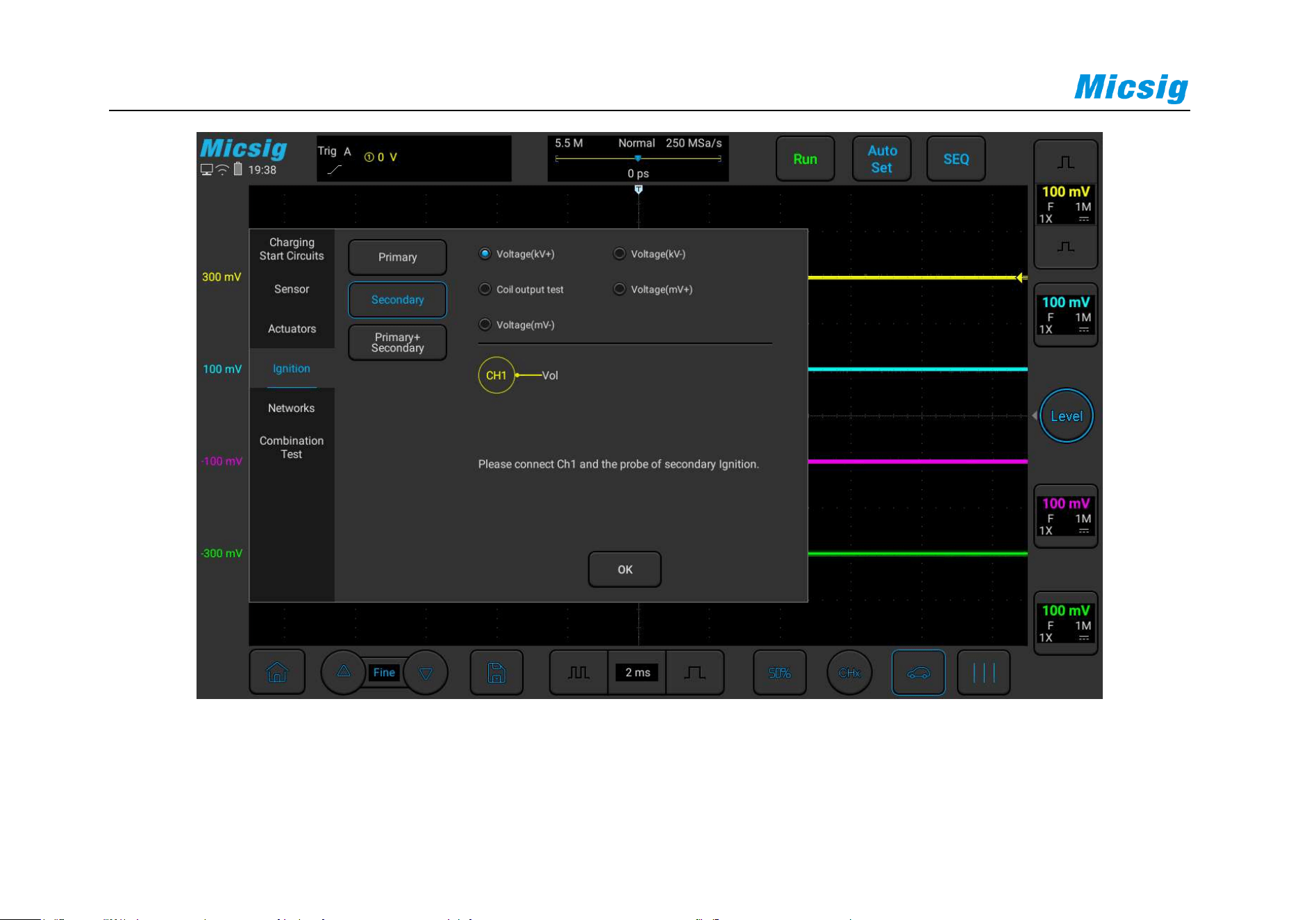
116
Figure 3-42 Secondary ignition test

Chapter 3 Automotive Test
117
3.4.3 Primary + Secondary
When measuring the primary and secondary waveforms at the same time, please use the P130A probe, one end is
connected to channel 1 of the oscilloscope, the black clip on the other end is grounded, pierce the needle into the
ground wire of the primary coil, and the probe is hooked to the metal needle; use a suitable secondary ignition
probe to connect one end to channel 2 of the oscilloscope, and test the other end according to different engine
ignition types.
Use ATO oscilloscope to simultaneously test the three indicators of the secondary ignition coil【Synchronize
voltage test of the primary and the secondary coil, Primary coil voltage and current, and the voltage of the
secondary coil ( use the secondary ignition probe)】, the specific operation is shown in the Figure 3-43:
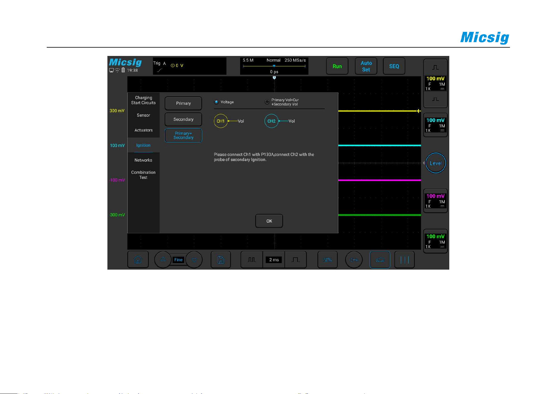
118
Figure 3-43: Primary + Scondary ignition test
The following figure is the actual measurement of the primary and secondary ignition of the BMW 5 Series N20
engine:
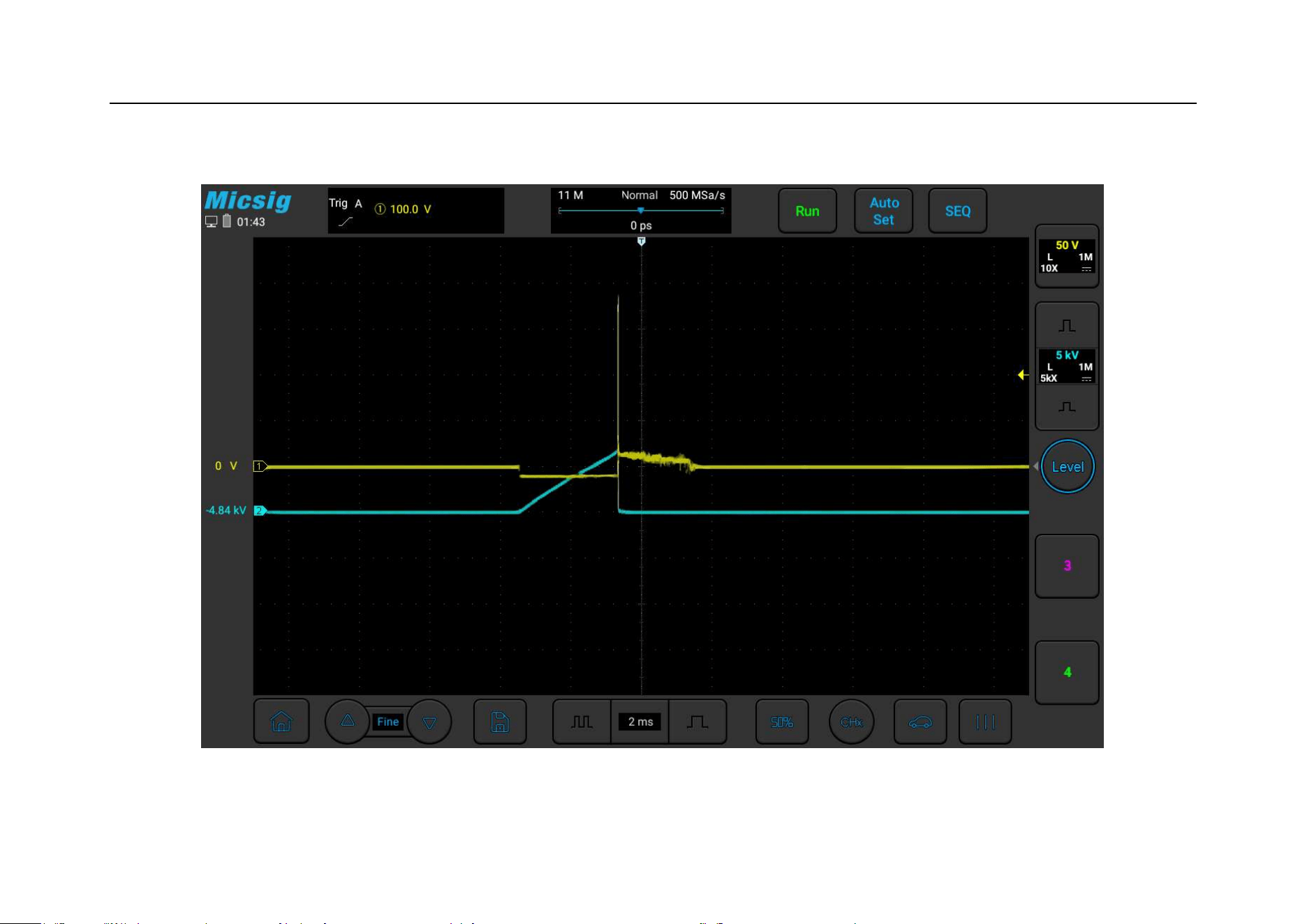
Chapter 3 Automotive Test
119
Figure 3-44 BMW 5 Series N20 Primary + Secondary ignition signal

120
3.5 Networks
3.5.1
CAN High & CAN Low
CAN bus is a communication system, which is widely used in modern vehicles. A car may have 2 to 3 CAN bus
networks, both high-speed and low-speed. The general high-speed transmission rate is 500k, which is usually used
for power transmission. The low-speed rate is 250k, which is usually used for meter transmission. Each CAN bus
network can connect multiple types of multiple devices, replacing the traditional multi-wire harness cable,
significantly reducing weight and increasing reliability.
The CAN bus has 2 wires, CAN high and CAN low, and the signals are in a differential relationship. The CAN bus
is divided into idle and transmission states. When idle, CAN high and CAN low are both 2.5V. When transmitting
signals, the high level of CAN high is 3.5V, and the low level is 2.5V; the high level of CAN low is 2.5 V, the low
level is 1.5V. Use a BNC to banana cable, one end is connected to channel 1 of the oscilloscope, the other end of the
black plug is grounded, and the red connector is pierced into the CAN high wire of the plug with a needle; use a
BNC to banana cable, one end is connected to channel 2 of the oscilloscope, and the other end is grounded, and the
red connector is pierced into the CAN low wire of the plug with a needle tip.
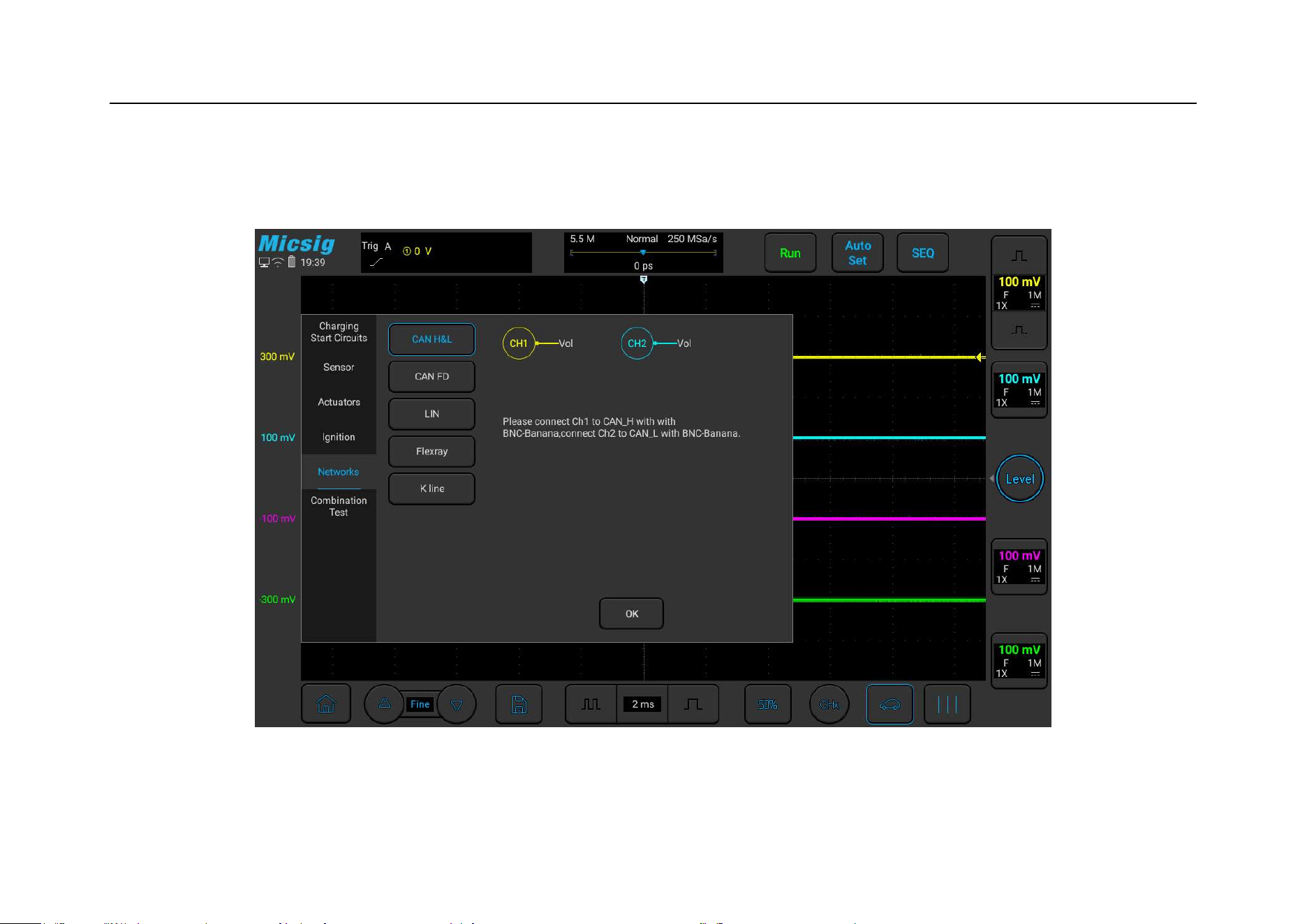
Chapter 3 Automotive Test
121
The specific CAN high and CAN low can be found in the technical manual of the vehicle.
Use ATO oscilloscope to test the CAN bus, the specific operation is shown in Figure 3-45:
Figure 3-45 CAN BUS Test
The figure below is the actual measurement of the CAN bus of a certain model:
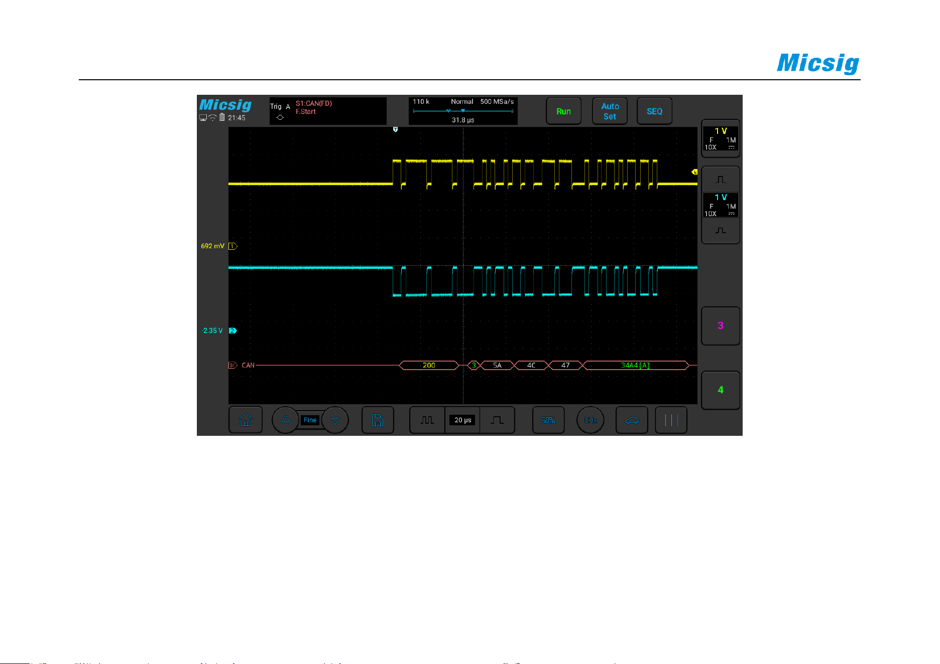
122
3.5.2 LIN Bus
The LIN protocol is short for Local Interconnect Network.
The Lin bus communication is very common in automobiles, it is low speed, there are multiple control devices
mounted on a network. It can contril non-safety-critical and low-speed devices on vehicles, such as wipers,
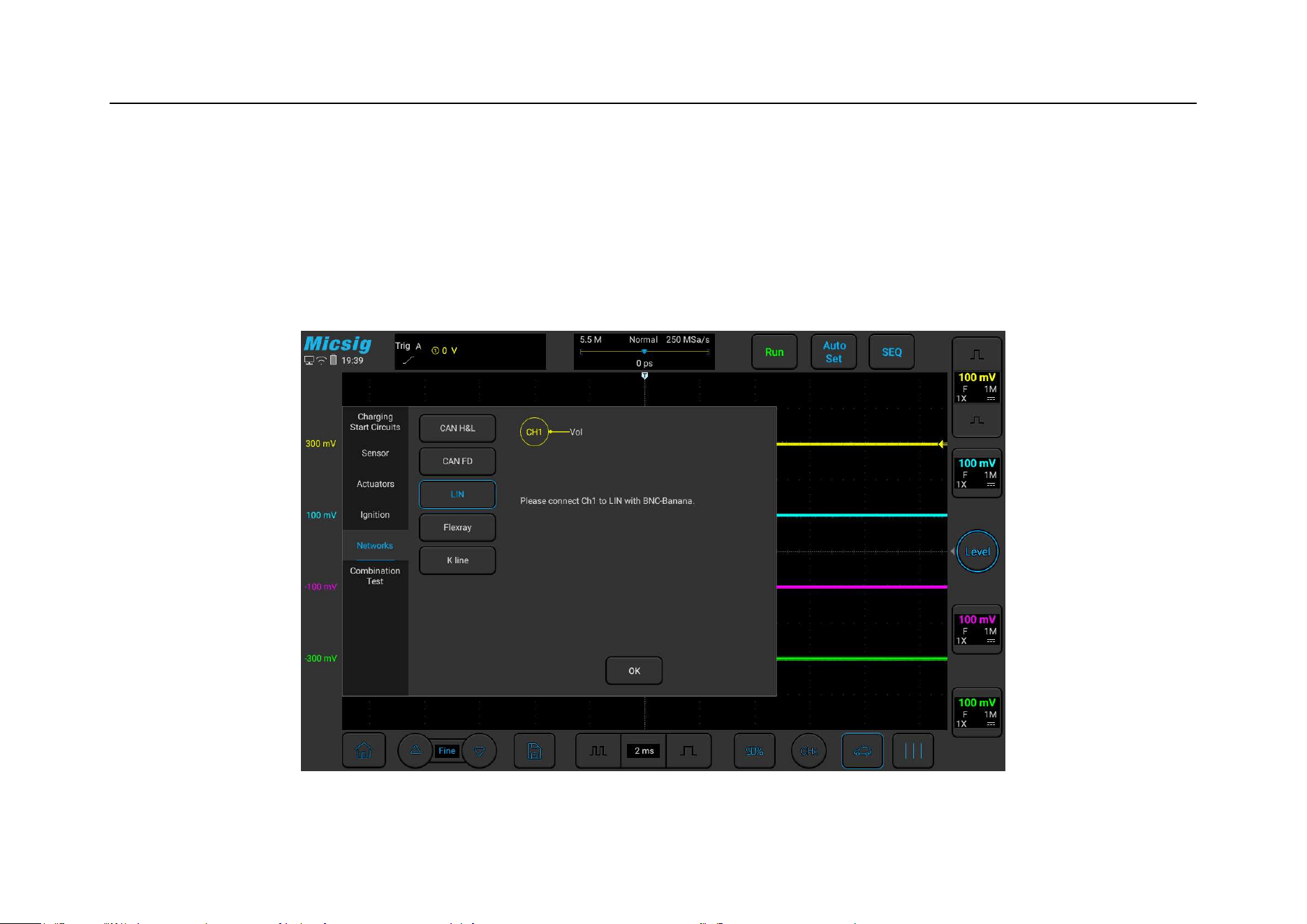
Chapter 3 Automotive Test
123
windows, mirrors, air conditioners, electronic seats, etc. LIN is single-wired, has high level and low level when
transmitting data, the high level is 12V, and the low level is 0V. The LIN bus generally has a sync header followed
by data. If there is only a signal from the sync header, it means that the device has not responded.
Use the ATO oscilloscope to test the LIN bus, the specific operation is shown in Figure 3-46:
Figure 3-46 Lin bus test
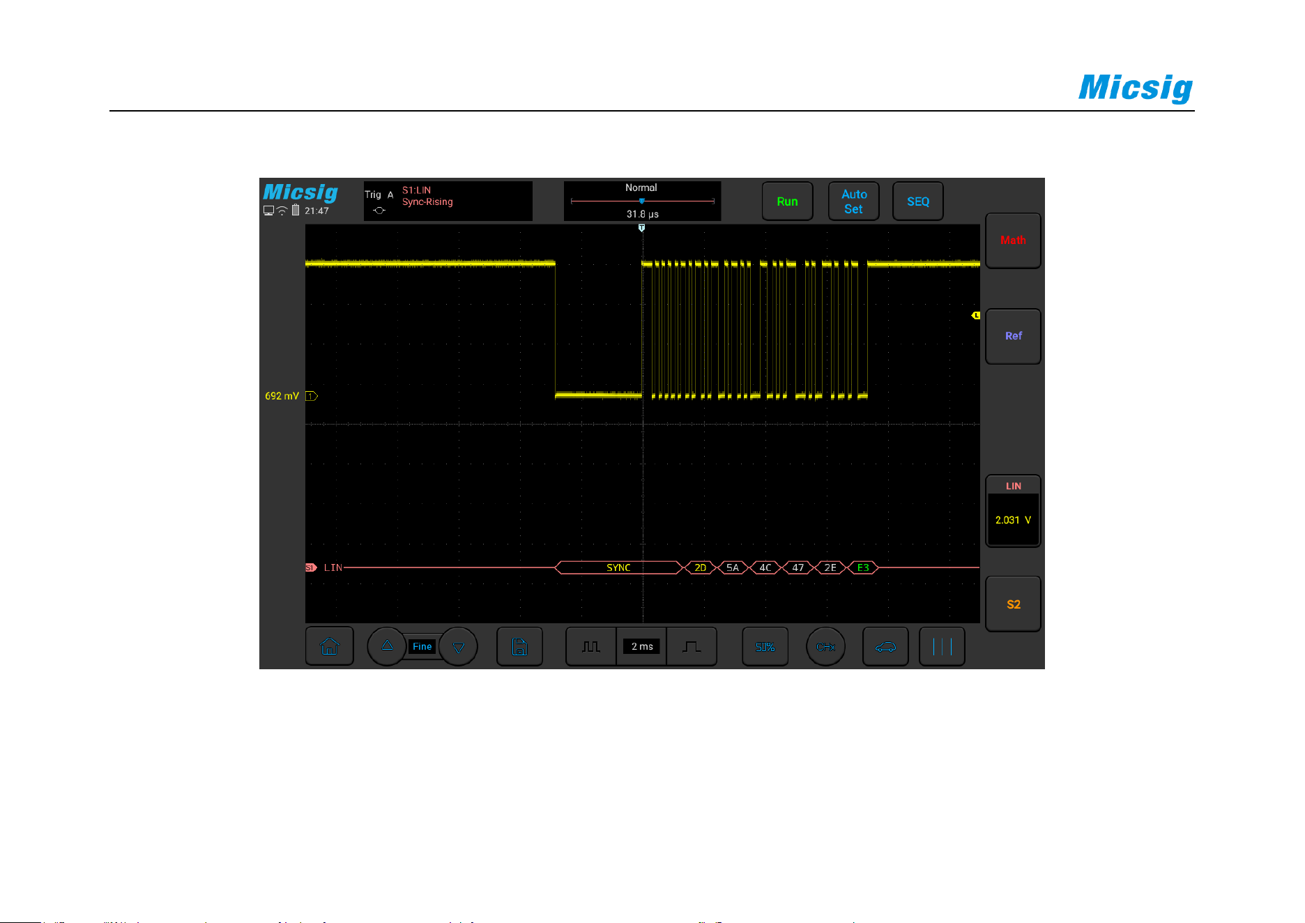
124
The following picture is the actual measurement of Audi A6 LIN bus in a certain year:
Figure 3-47 Audi A6 LIN bus measurement

Chapter 3 Automotive Test
125
3.5.3 FlexRay Bus
With the increase of car transmission content, the Flexray bus with faster transmission speed has been developed,
and the transmission rate can reach 10Mbps. It has the advantages of high speed, determinability, and fault
tolerance. It can work with CAN, LIN and other buses.
The Flexray bus still has 2 lines and the waveform is in a differential pattern. When idle, the voltage of the two
wires is 2.5V; when transmitting data, both wires will have a voltage of 1V up and down, and the voltages on the
two wires are opposite.
Use the P130A probe, one end is connected to channel 1 of the oscilloscope, and the other end is grounded with the
black clip. Use a piercing needle to pierce the easy-to-test Flexray bus positive plug, and hook the probe to the
metal needle of the puncture needle. Use the P130A probe, connect one end to channel 2 of the oscilloscope, and
the black clip on the other end to ground. Use a needle to pierce the easy-to-test Flexray bus negative plug, and
hook the probe to the metal needle of the needle.
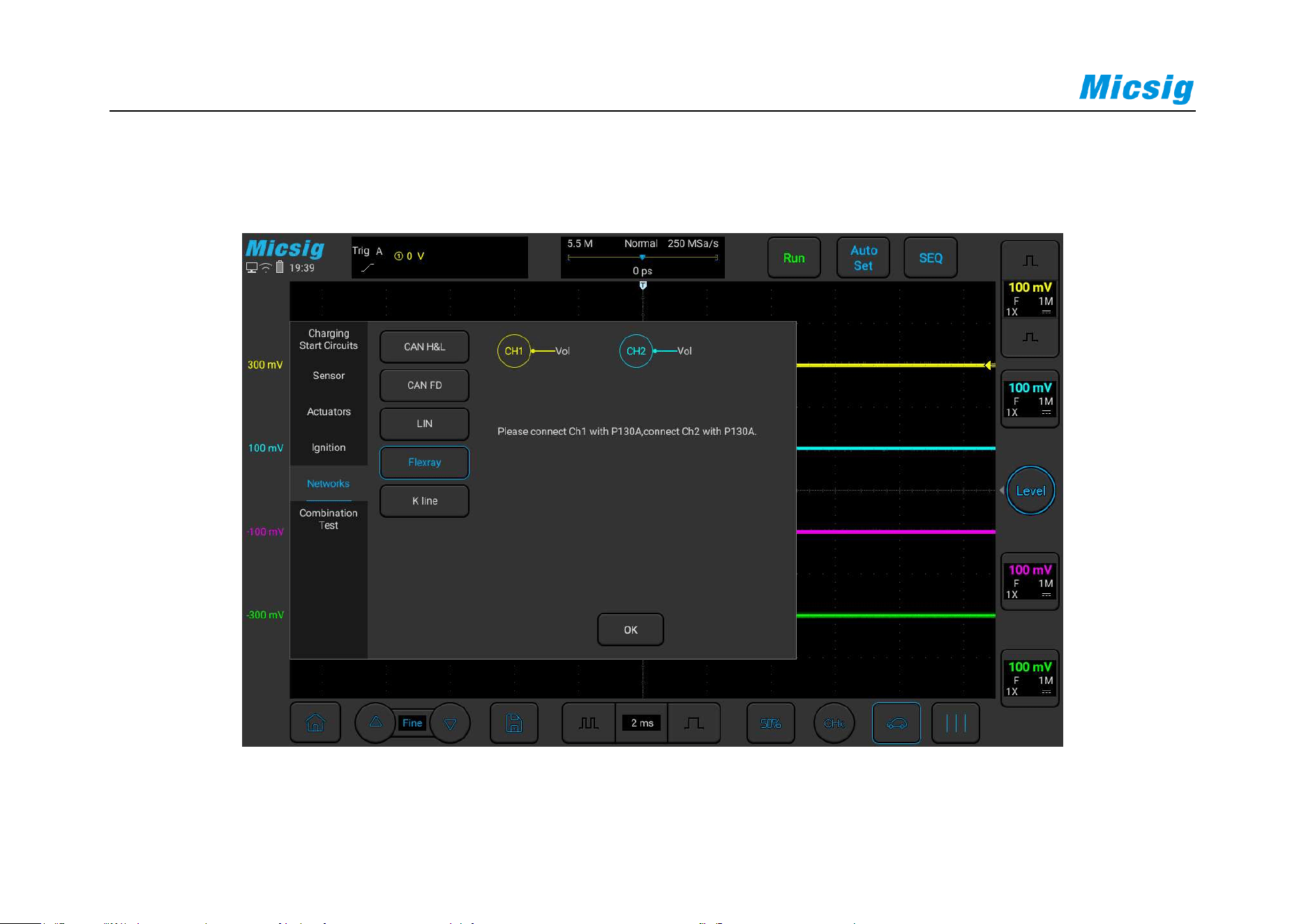
126
The specific Flexray bus measurement location can be found in the vehicle's technical manual.
Use the ATO oscilloscope to test the FlexRay bus, the specific operation is shown in Figure 3-48:
Figure 3-48: FlexRay bus test

Chapter 3 Automotive Test
127
3.5.4 K line
The K line is a special line for data transmission between the car control unit and the diagnostic instrument, and the
transmission rate is low. In general, K-Line is very different from CAN Bus and most communication networks. For
example, the CAN Bus network does not have a central or master ECM: all ECMs are equal because they can send
and receive information along the network. The K line has only one line, and the information is transmitted in
binary format and the pulse voltage signal is transmitted. Divided into 0 and 1, 0 is high level, 12V or above, 1 is
low level, voltage is 0V.
Use the ATO oscilloscope to test the K line, the specific operation is shown in Figure 3-49 below:
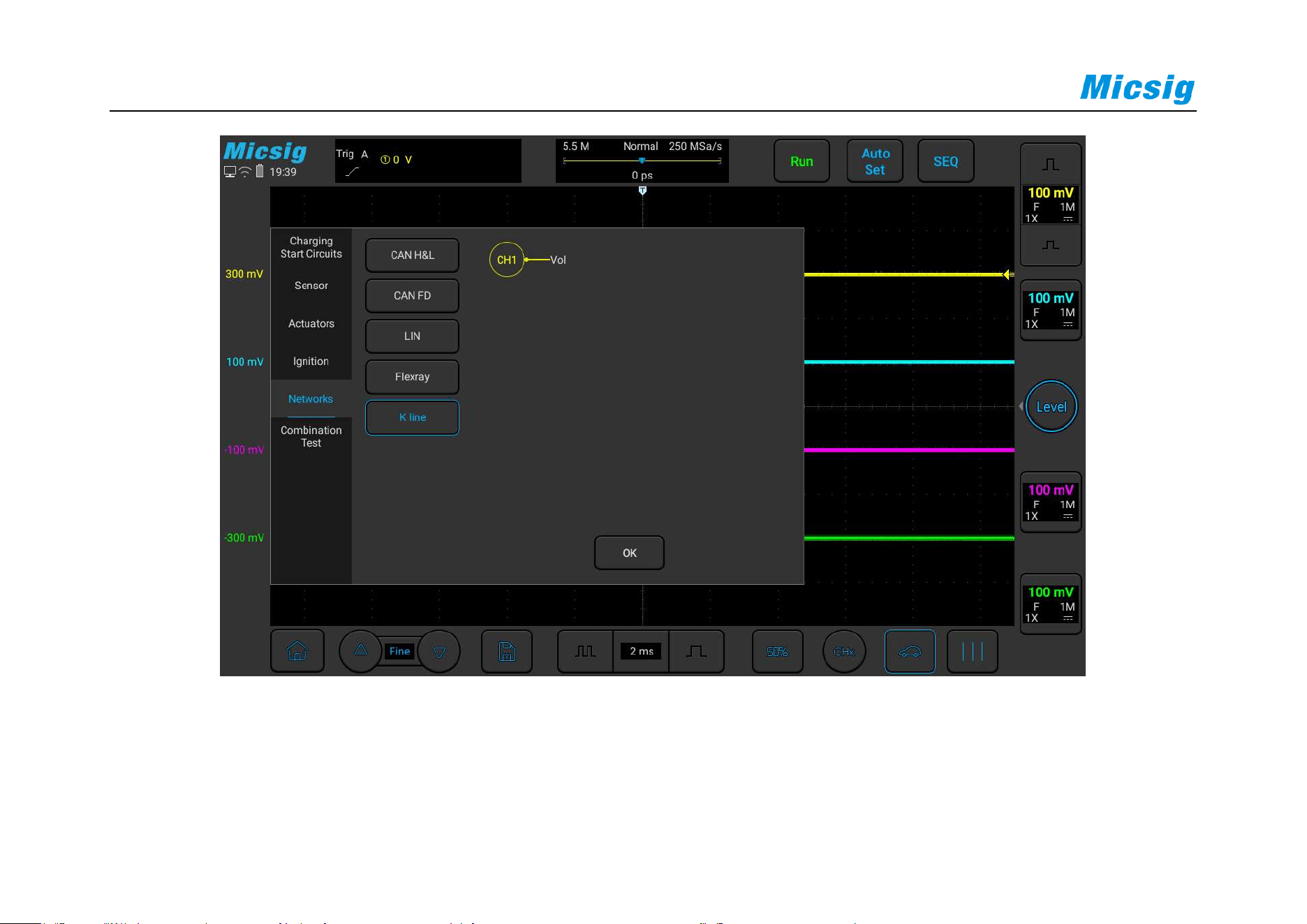
128
Figure 3-49 K line test

Chapter 3 Automotive Test
129
3.6 Combination Tests
The electronic faults of automobiles are sometimes more complicated. We need to use an ATO oscilloscope to
perform combination testing, compare several waveforms that collected, and help users judge the fault by observing
and analyzing the timing relationship and quantitative relationship between the waveforms. The ATO is a powerful
tool to solve such complex problems.
3.6.1
Crankshaft + Camshaft
Use a BNC to banana cable, one end is connected to channel 1 of the oscilloscope, the other end is grounded with a
black plug, and the red connector is pierced into the signal line of the crankshaft sensor with a needle; use a BNC to
banana cable, one end is connected to channel 2 of the oscilloscope, and the other black end is grounded, the red
connector is pierced into the signal line of the camshaft sensor with a needle probe.
Use ATO oscilloscope to perform combined test on crankshaft + camshaft, the specific operation is shown in Figure
3-50:
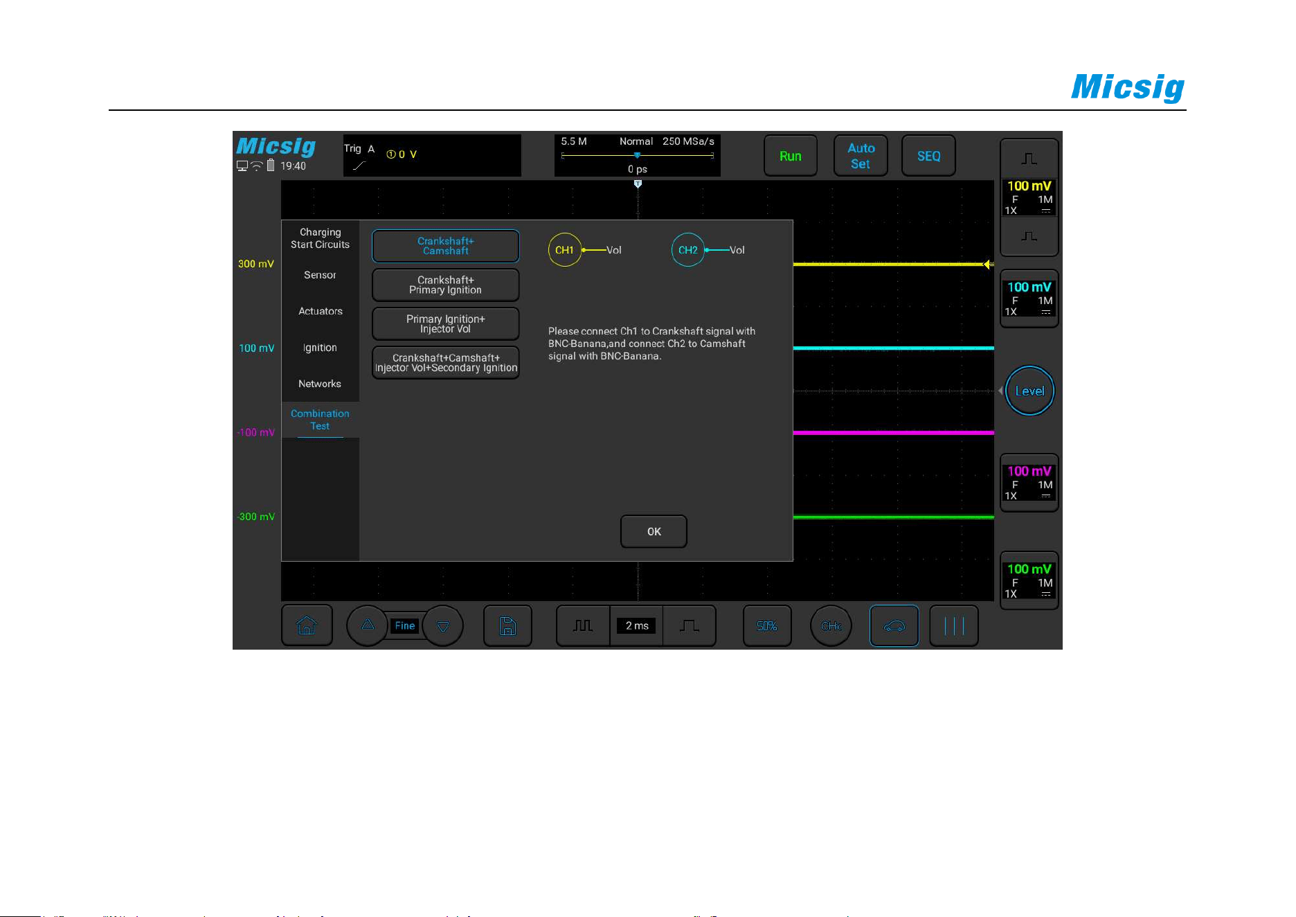
130
Figure 3-50 Crankshaft + Camshaft Combination Test

Chapter 3 Automotive Test
131
3.6.2 Crankshaft + Primary ignition
Measure the crankshaft and primary ignition at the same time, you can check whether the ignition advance angle is
normal, and look for the cause of misfire at high engine speed. Check whether the crankshaft signal is normal or
whether the primary ignition voltage and closing time are reached.
Use a P130A probe, one end is connected to channel 1 of the oscilloscope, and the other end is grounded with a
black clip. Use a needle to pierce the signal line at the end of the injector plug, and hook the probe to the metal
needle of the needle;
Use a P130A probe, connect one end to channel 2 of the oscilloscope, and the black clip on the other end to ground.
Use a needle to pierce the ground wire of the primary coil, and hook the probe to the metal needle of the needle;
Use ATO oscilloscope to perform combined test on crankshaft + primary ignition, the specific operation is shown in
Figure 3-51:

132
Figure 3-51 Crankshaft + Primary ignition test

Chapter 3 Automotive Test
133
3.6.3 Primary ignition + Injector voltage
If there is a problem with the startup or it is suddenly off, it may be necessary to test the primary ignition and the
fuel injector at the same time. If the primary ignition fails, no fuel injector signal will be generated.
Use a P130A probe, one end is connected to channel 1 of the oscilloscope, and the other end is grounded with a
black clip. Use a needle to pierce the signal line at the end of the injector plug, and hook the probe to the metal
needle of the needle;
Use the P130A probe, one end is connected to channel 2 of the oscilloscope, and the other end is grounded with the
black clip. Use a puncture needle to pierce the ground wire of the primary coil, and hook the probe to the metal
needle of the puncture needle.
Use the ATO oscilloscope to perform a combined test on the primary ignition + injector voltage, the specific
operation is shown in Figure 3-52:
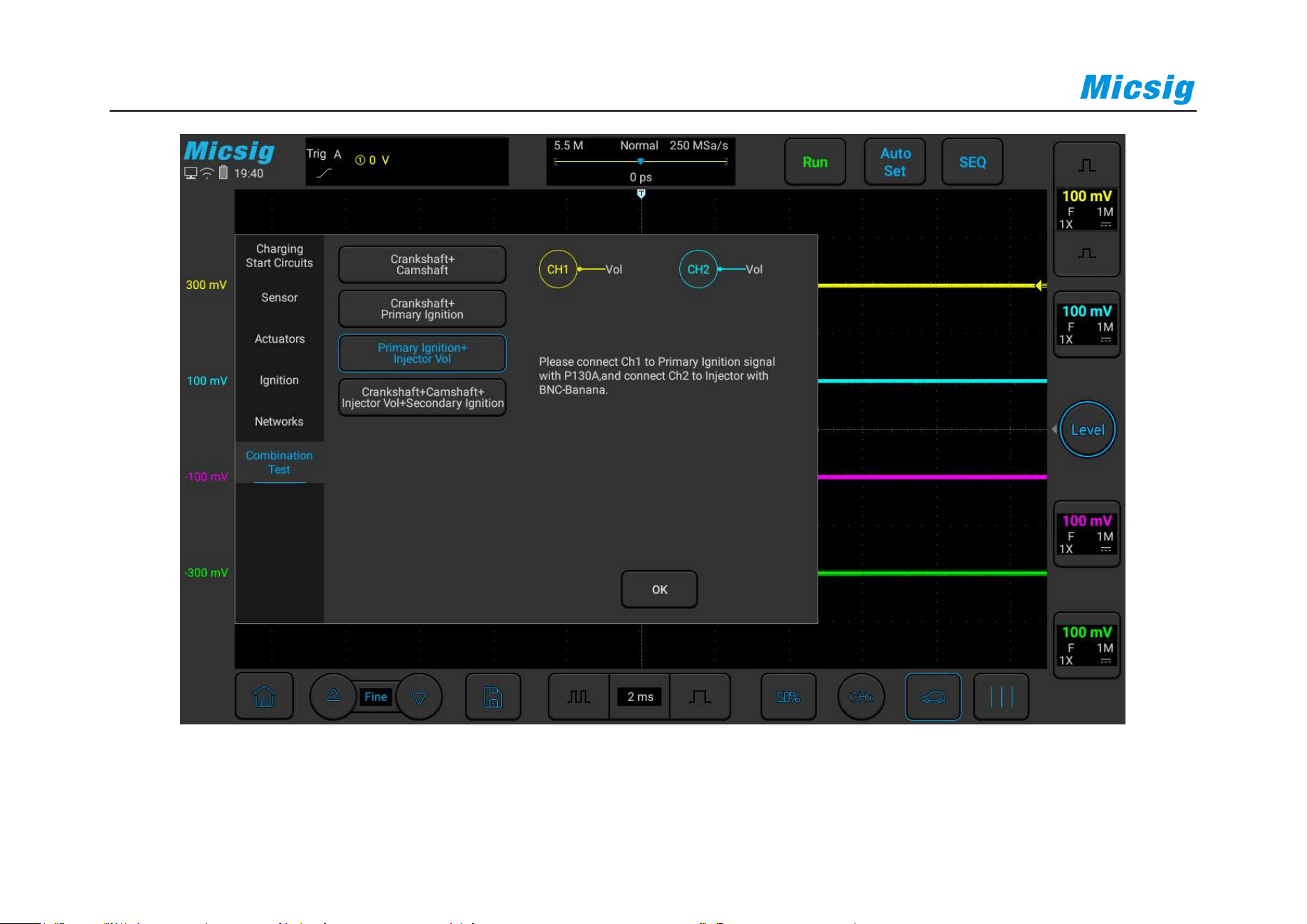
134
Figure 3-52 Primary ignition + Injector voltage

Chapter 3 Automotive Test
135
3.6.4 Crankshaft + Camshaft + Injector + Secondary Ignition
Use a BNC to banana cable, one end is connected to channel 1 of the oscilloscope, the other end is grounded with a
black plug, and the red connector is pierced into the signal line of the crankshaft sensor with a needle;
Use a BNC to banana cable, one end is connected to channel 2 of the oscilloscope, the other end is grounded with a
black plug, and the red connector is pierced into the signal line of the camshaft sensor with a needle;
Use a P130A probe, one end is connected to channel 3 of the oscilloscope, and the other end is grounded with a
black clip. Use a needle to pierce the signal line at the end of the injector plug, and hook the probe to the metal
needle of the needle;
Use a suitable secondary ignition probe, connect one end to channel 4 of the oscilloscope, and connect the other end
to the secondary ignition part of the vehicle.
Turn on the key, start the vehicle, and check the waveform.
ATO oscilloscope can be used to perform combined test on crankshaft + camshaft + fuel injector + secondary
ignition. The specific operation is shown in Figure 3-53.
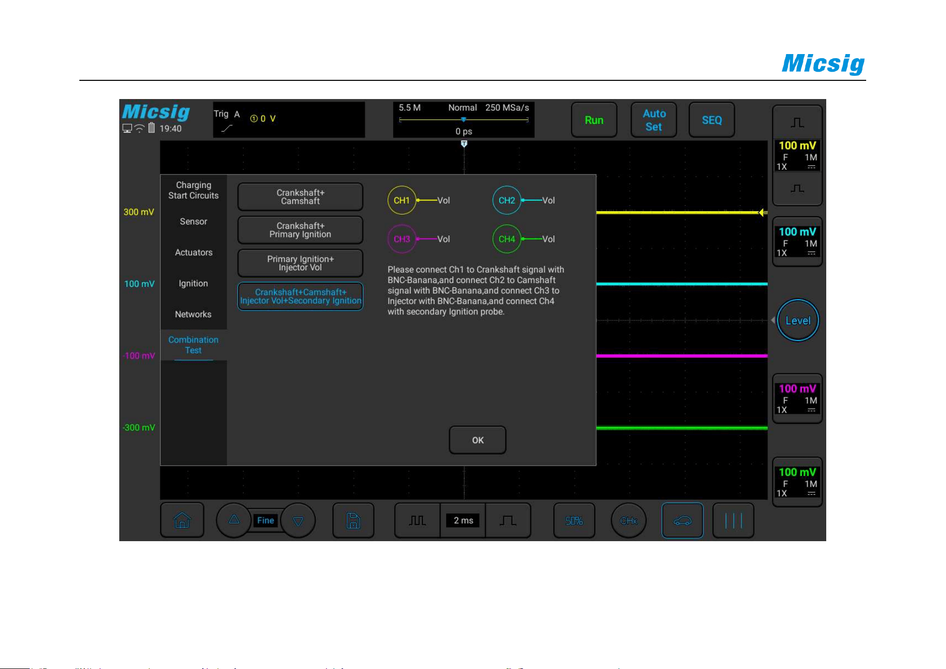
136
Figure 3-53 Combination test of Crankshaft + Camshaft + Injector + Secondary ignition

Chapter 4 Horizontal System
137
Chapter 4 Horizontal System
This chapter contains the detailed information of the horizontal system of the oscilloscope. You are recommended
to read this chapter carefully to understand the set functions and operation of the horizontal system of the ATO
series oscilloscope.
Move the waveform horizontally
Adjust the horizontal time base (time/div)
Pan and zoom single or stopped acquisitions
Roll, XY
Zoom mode
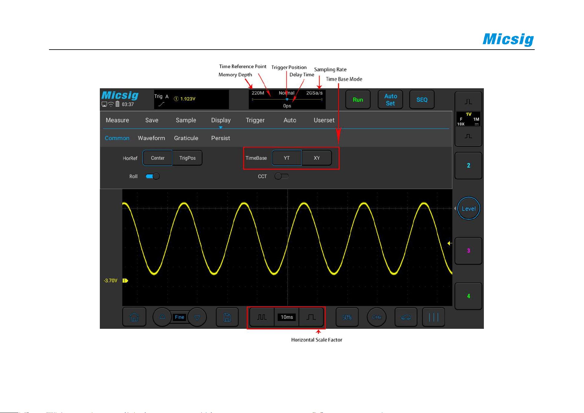
138
Figure 4-1 Horizontal system
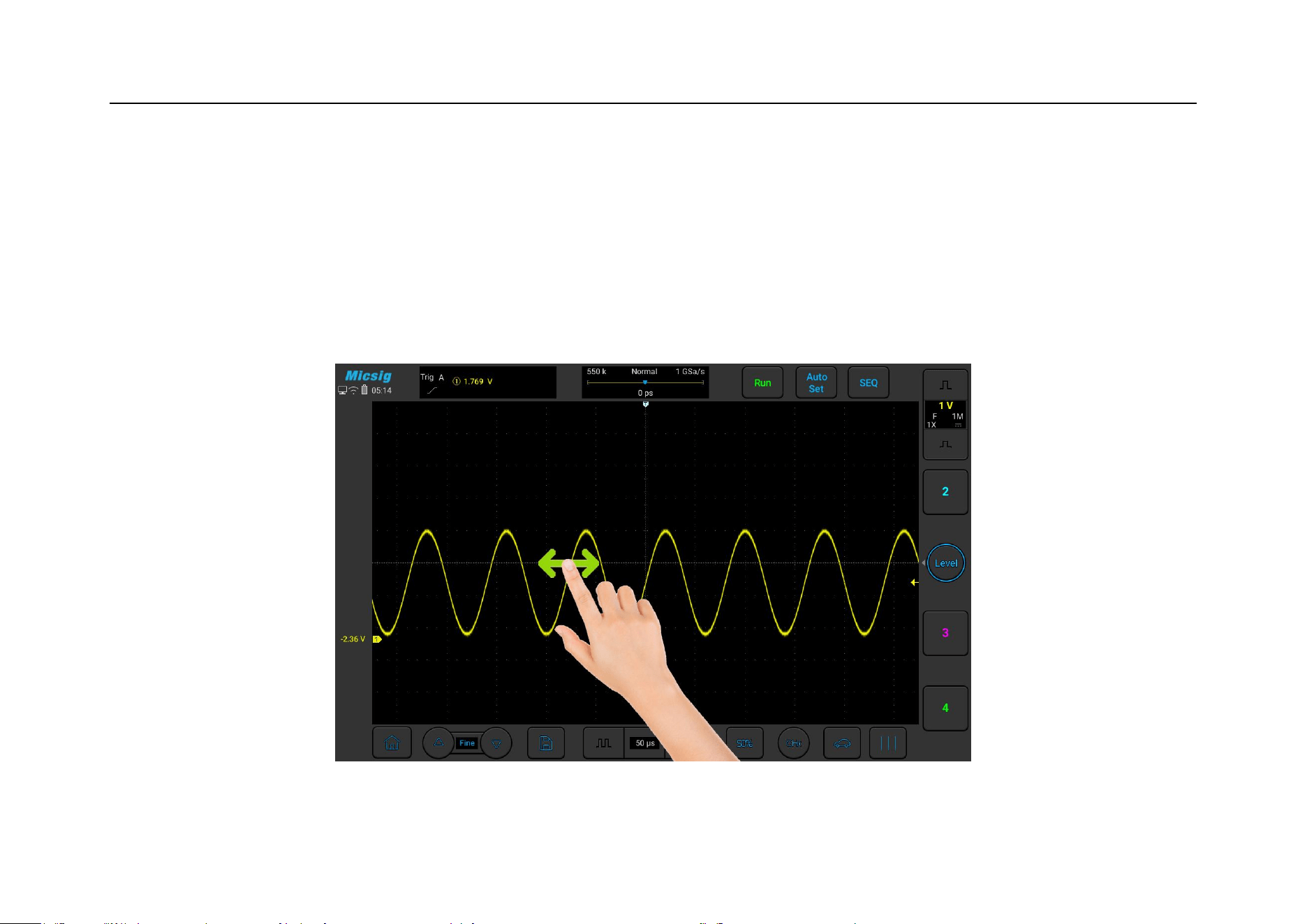
Chapter 4 Horizontal System
139
4.1 Move the Waveform Horizontally
Put one finger on the waveform display area to swipe left and right, for the coarse adjustment of the waveform
position horizontally of all analog channels; after moving the waveform, tap the fine adjustment button in the lower
left corner of the screen for fine adjustment.
Figure 4-2 Move the Waveform Horizontally on the Screen

140
4.2 Adjust the Horizontal Time Base (time/div)
Method 1: Soft Keys
Tap , buttons to adjust the horizontal time base of all analog channels (current channels). Tap button
to increase the horizontal time base; tap button to zoom out the horizontal time base (see Figure 4-3 Adjust the
Horizontal Time Base). The horizontal time base is stepped in 1-2-5, while the waveform changes as the time base
changes.
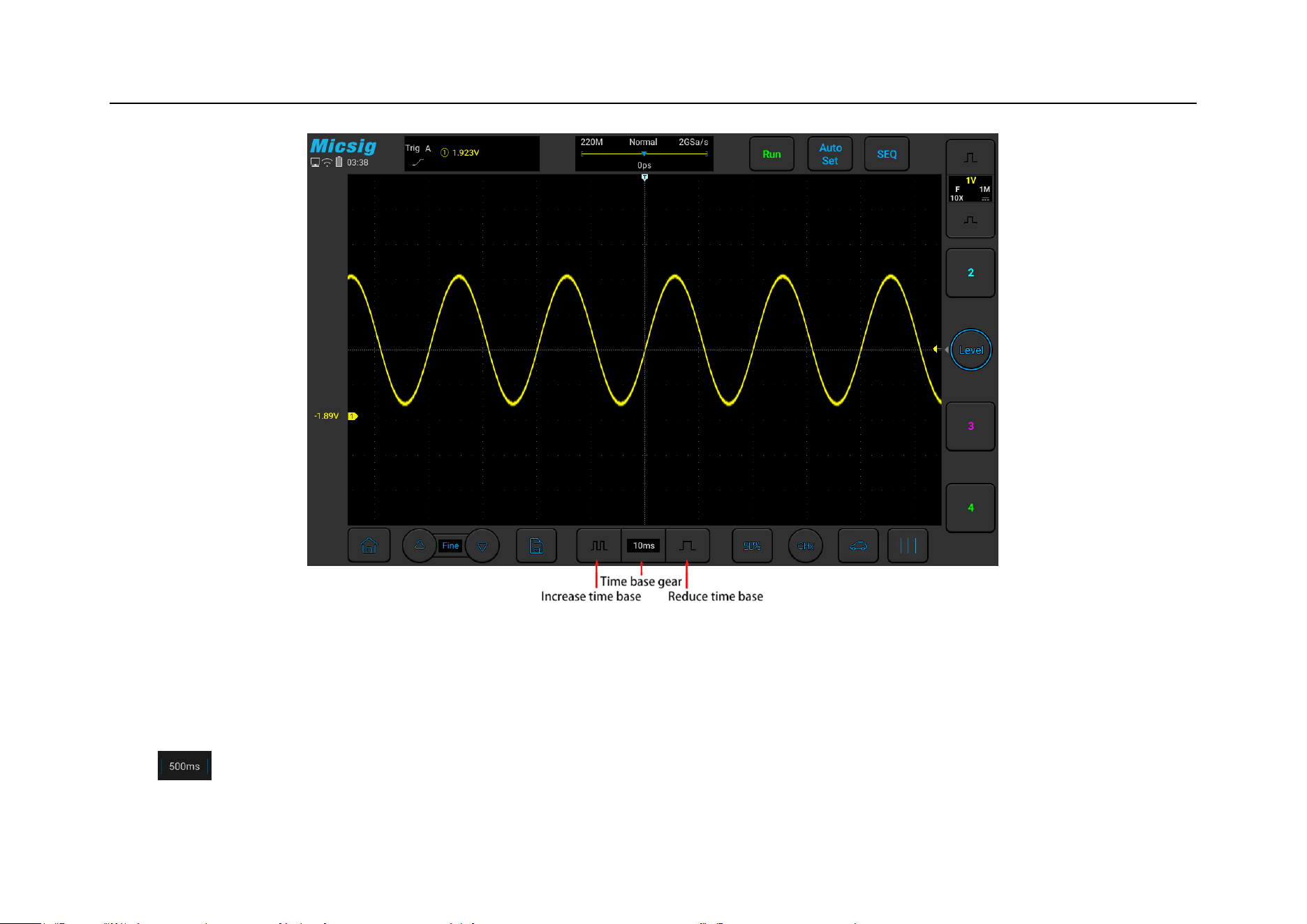
Chapter 4 Horizontal System
141
Figure 4-3 Adjust the Horizontal Time Base
Method 2: Time Base Knob
Tap to open the time base list (see Figure 5-4 Horizontal Time Base List), then tap the list to select the
appropriate time base. The time base with the blue filled background is the currently selected time base.
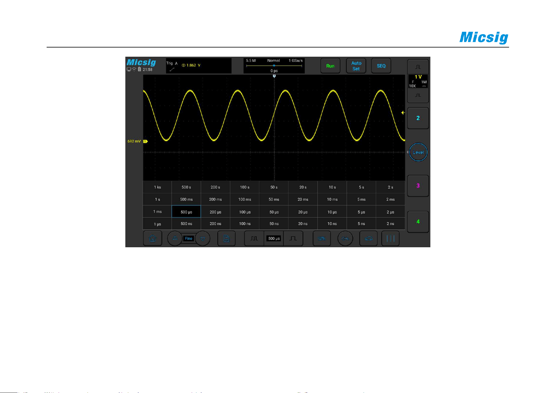
142
Figure 4-4 Horizontal Time Base Knob
4.3 Pan and Zoom Single or Stopped Acquisitions
After the oscilloscope is stopped, the stopped display screen may contain several acquired data with useful
information, but only the data in the last acquisition can be horizontally moved and zoomed. The data of the single
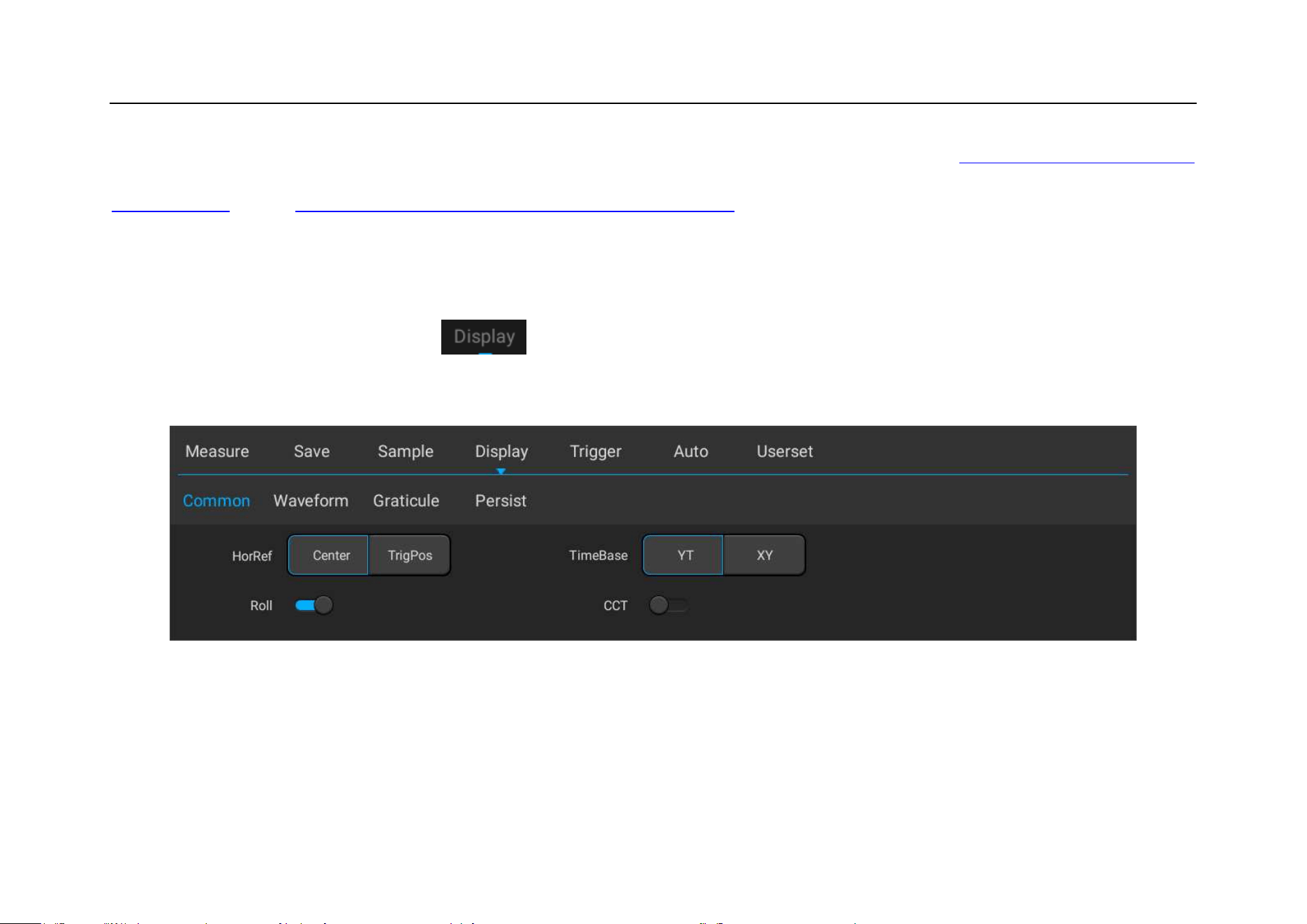
Chapter 4 Horizontal System
143
acquisition or stopped acquisition is moved horizontally and zoomed. For details, refer to “5.1 Move the Waveform
Horizontally” and “5.2 Adjust the Horizontal Time Base (time/div)”.
4.4 Roll, XY
In the main menu, tap the soft key , then select the desired time base mode. The time base mode is divided
into YT, ROLL, and XY.
Figure 4-5 Display Mode
YT——Normal View Mode of Oscilloscope

144
In YT mode, the relative relationship between vertical voltage and horizontal time is displayed. Y axis represents
the voltage, X axis represents the time, and the waveform is displayed after triggering (waveform displayed from
left to right).
Note: When the time base is large (such as 200ms and above), sometimes the waveform will not be displayed for a
long time; this is because in YT mode, the waveform must be triggered before display. It is closely related to the
time base and can be roughly calculated as: the number of divisions on the left side of the trigger position * time
base level position; if you want to reduce the waiting time, move the trigger position to the left.
The case that trigger position is moved out of the waveform screen is not considered here.
ROLL—— ROLL Mode
In ROLL mode, the waveform rolls from right to left to refresh the display (see Figure 4-6 ROLL Mode). The
horizontal time base adjustment range of the ROLL mode in the running state is 200ms/div~1ks/div.
In ROLL mode, trigger related information is invalid, including trigger position, trigger level, trigger voltage, etc.
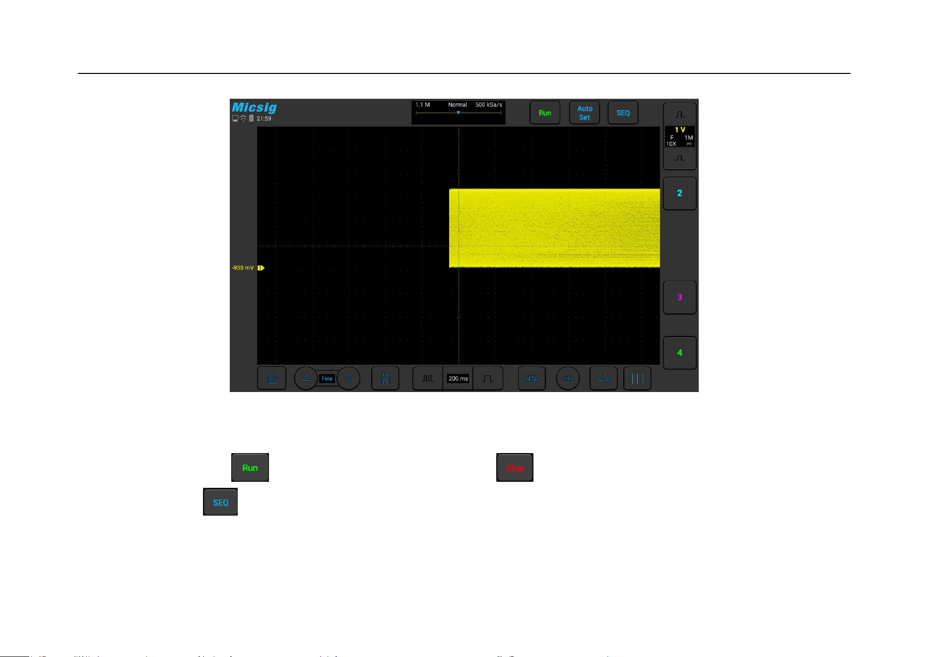
Chapter 4 Horizontal System
145
Figure 4-6 ROLL Mode
In ROLL mode, press to stop waveform display; press again to clear waveform display and restart
acquisition; press to execute single sequence, it will stop automatically after completing a full screen
acquisition.
ROLL mode is generally used to observe waveforms with frequencies below 5 Hz.
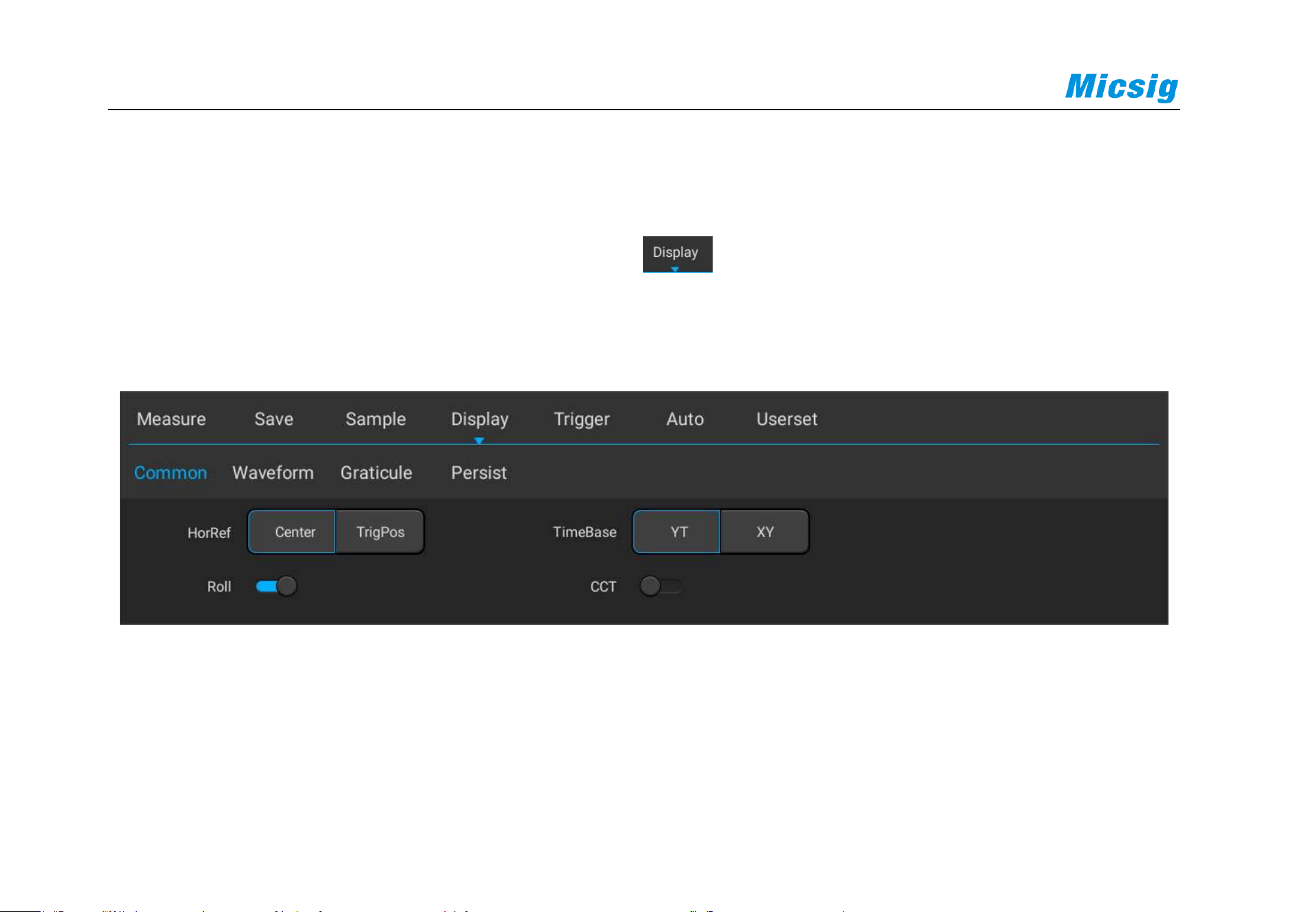
146
ROLL mode is defaulted as open. When the time base is greater than 100ms, it automatically enters the ROLL
mode. If the signal to be triggered under a large time base needs to be viewed, turn off the ROLL mode.
Roll mode on and off: In the main menu, tap the soft key . In the “Common” option, you can turn the roll
mode on and off (refer to Figure 4-7). When the roll mode is on and the time base is within 200ms~1ks, the
oscilloscope automatically enters the roll mode.
Figure 4-7 Roll Mode On/Off

Chapter 4 Horizontal System
147
XY——XY Mode
The vertical amount of CH1 is displayed on the horizontal axis in XY mode, and the vertical amount of CH2 is
displayed on the vertical axis (see Figure 4-8 XY Mode).
You can use XY mode to compare the frequency and phase relationship of two signals.
XY mode can be used for sensors to display stress-displacement, flow-pressure, voltage-frequency or voltage-
current, for example: plotting a diode curve.
You can also use the cursor to measure the waveform in XY mode.
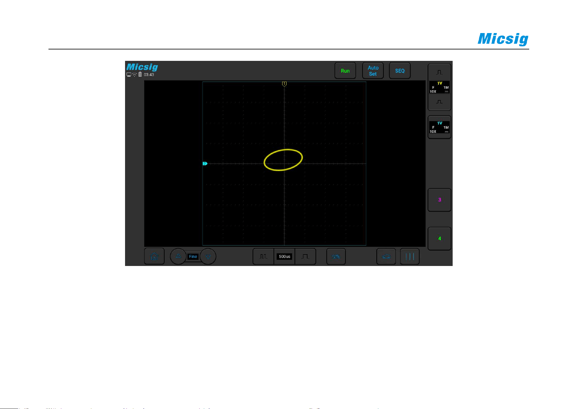
148
Figure 4-8 XY Mode
XY Mode Example
This exercise shows the usual practice of XY display mode by measuring the phase difference between two signals
of the same frequency using the Lissajous method.

Chapter 4 Horizontal System
149
1) Connect sine wave signals to CH1 and connect sine wave signals of the same frequency and different phases to
CH2.
2) Press “Auto” set button, tap “Display” in the main menu, then select “XY” in “Time Base”.
3) Drag signals so that they are centered on the display screen. Adjust the vertical sensitivity of CH1 and CH2,
and extend signals for viewing.
The phase difference (θ) can be calculated using the following formula (assuming that the amplitudes of the
two channels are the same):
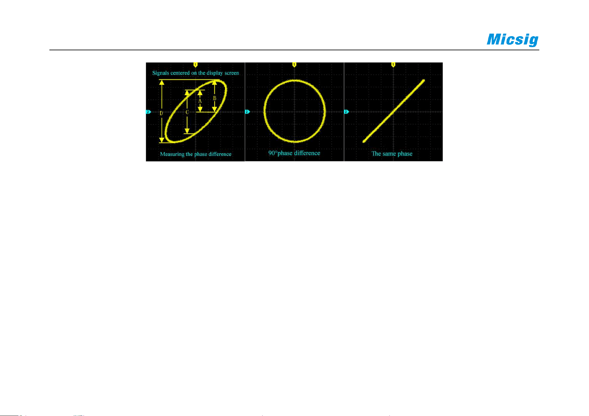
150
Figure 4-9 XY Time Base Mode Signal, Center on the Display Screen
4) Tap the “Cursor” button to open the horizontal cursor.
5) Set the cursor y2 at the top of the signal and the cursor y1 at the bottom of the signal. Record the Δy value in
the upper right corner of the screen.
6) Move y1 and y2 cursors to the intersection point of the signal and the y-axis. Record the Δy value again.
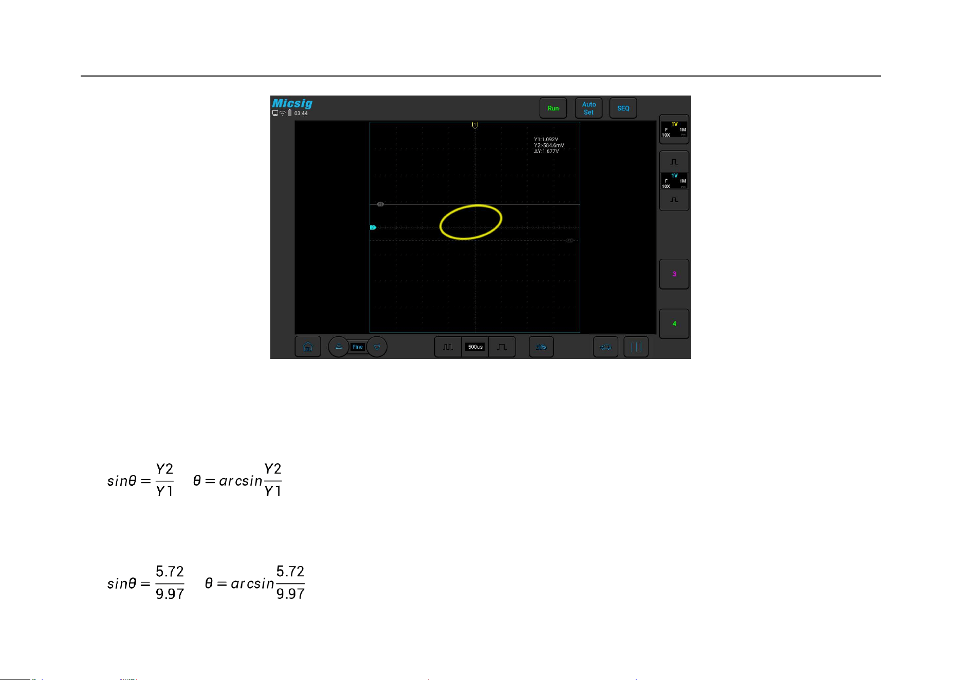
Chapter 4 Horizontal System
151
Figure 4-10 Phase Difference Measurement and Using the Cursor
7) The following formula is used to calculate the phase difference.
;
For example, if the first Δy value is 9.97V, the second Δy value is 5.72V:
;
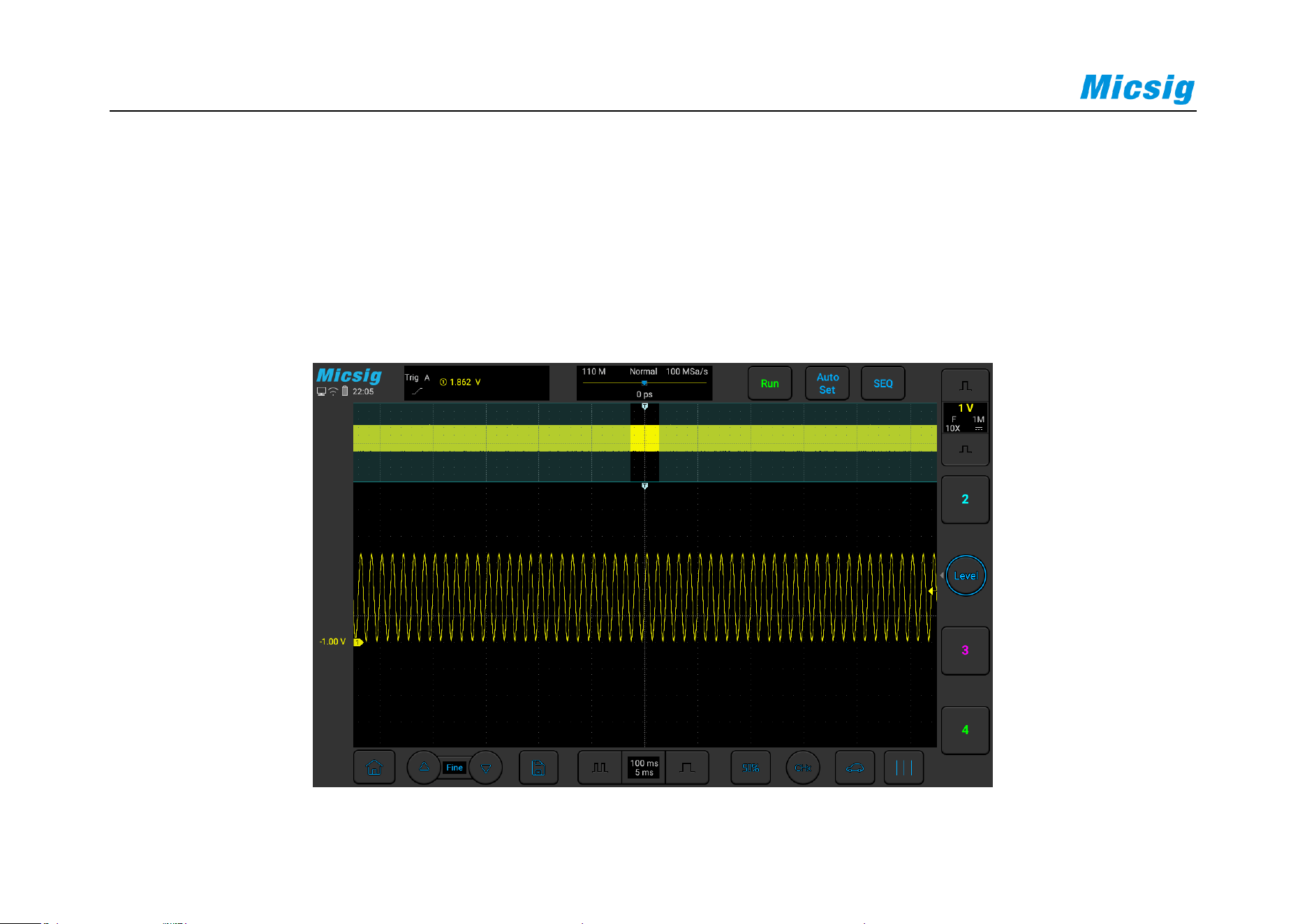
152
4.5 Zoom Mode
Zoom is a horizontally expanded version of the normal display. Open the zoom function, the display is divided into
two parts (see Figure 4-11 Zoom Interface). The upper part of the display screen shows the normal display window
view and the lower part shows the zoomed display window.
Figure 4-11 Zoom Interface

Chapter 4 Horizontal System
153
Zoom window view is the enlarged portion of the normal display window. You can use “Zoom” to view a portion
of the normal window that is horizontally expanded to learn more about signal analysis.
Zoom on/off:
Open the pull-up menu and tap button to turn the zoom function on/off.
Zoom window is framed in a box on the normal window, and the other portion is covered by gray shade not
displayed in the zoom window. This box shows the normal scan portion that was zoomed in the lower bottom.
Tap the time base button to adjust the time base of the zoom window. The size of the box in the normal window
changes according to the time base of the zoom window.
Drag the waveform of the zoom window horizontally to adjust the waveform position. The box in the main window
moves oppositely against the waveform; or directly drag the box in the normal window to quickly locate the
waveform to be viewed.
Note:

154
1) The minimum time base is displayed in the normal window when the waveform in the screen is exactly within
the memory depth. If the current time base is smaller than the minimum time base in the normal window at the
current memory depth, when the zoom window is opened, the time base in the normal window is automatically
set to the minimum time base in the normal window at the current memory depth.
2) The cursor, math waveform, and reference waveform are not displayed in the normal window, but can be
displayed in the Zoom window.
3) If Roll mode is stopped, Zoom mode can be turned on, and tap “Run/Stop” to automatically turn off Zoom
mode.

Chapter 5 Vertical System
155
Chapter 5 Vertical System
This chapter contains the detailed information of the vertical system of the oscilloscope. You are recommended to
read this chapter carefully to understand the set functions and operation of the vertical system of the ATO series
oscilloscope.
Open/close channel, set the current channel
Set probe type
Adjust vertical sensitivity
Set probe attenuation coefficient
Adjust vertical position
Vertical expansion reference
Open channel menu
Set channel coupling
Set bandwidth limit
Waveform inversion
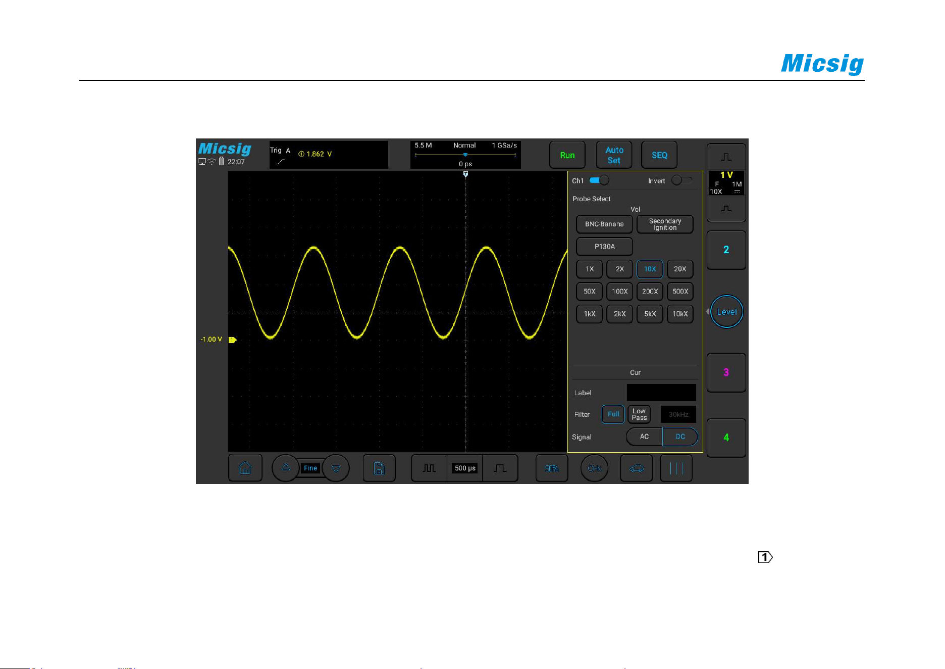
156
The figure below shows the “CH1 Channel Menu” displayed after opening the CH1 channel menu.
Figure 5-1 Channel Menu Display Interface
The ground level of each displayed analog channel signal is indicated by the channel indicator icon on the far
left of the display screen.
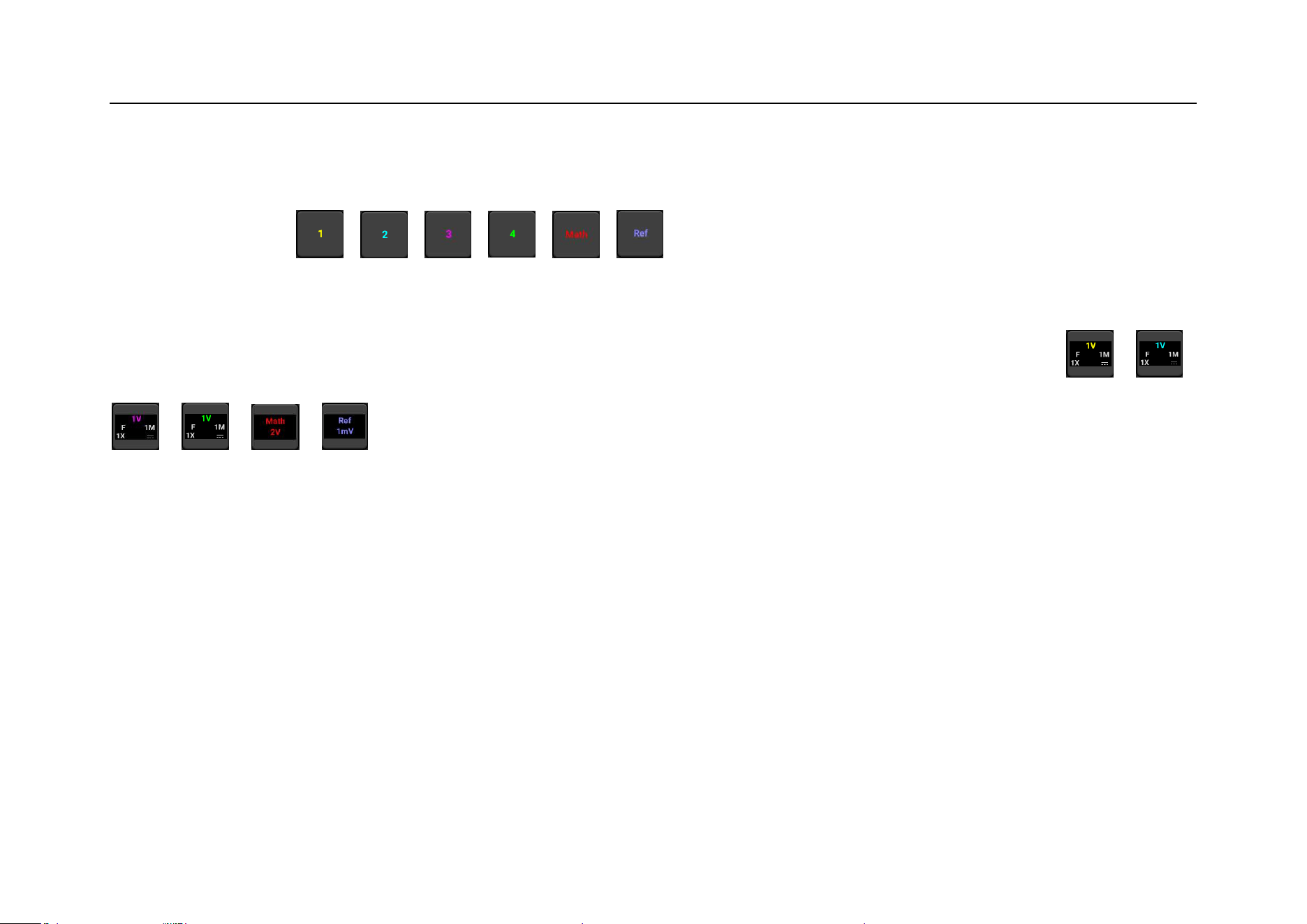
Chapter 5 Vertical System
157
5.1 Open/Close Waveform (Channel, Math, Reference Waveforms)
The channel icons , , , , , on the right side of the oscilloscope waveform display
area (swipe up or down to switch to math channel and reference channel) correspond to the six channels of CH1,
CH2, CH3, CH4, math function and reference channel. The channel icons in open state will shows like , ,
, , , . Swipe right to close the desired channel.
Current channel: The oscilloscope can display multiple waveforms at the same time, but only one waveform is
preferentially displayed on the uppermost layer, and the channel that is preferentially displayed on the uppermost
layer is called the current channel. The channel indicator for the current channel is solid, and the channel indicator
for the non-current channel is hollow, as shown in Figure 5-2.
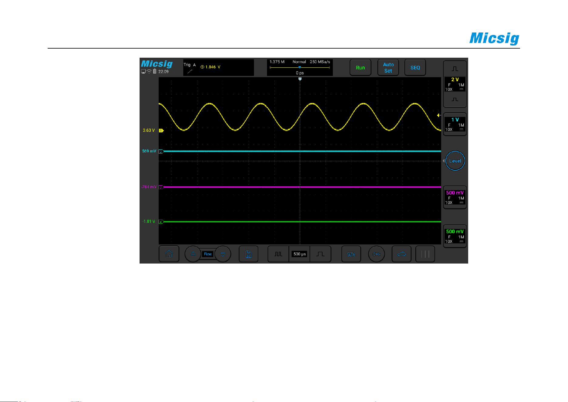
158
Figure 5-2 Current Channel and Non-Current Channel
The display content of the oscilloscope channel display interface includes the vertical scale, vertical scale
sensitivity button, coupling mode, invert, bandwidth limitation of the channel, as shown in Figure 5-3.
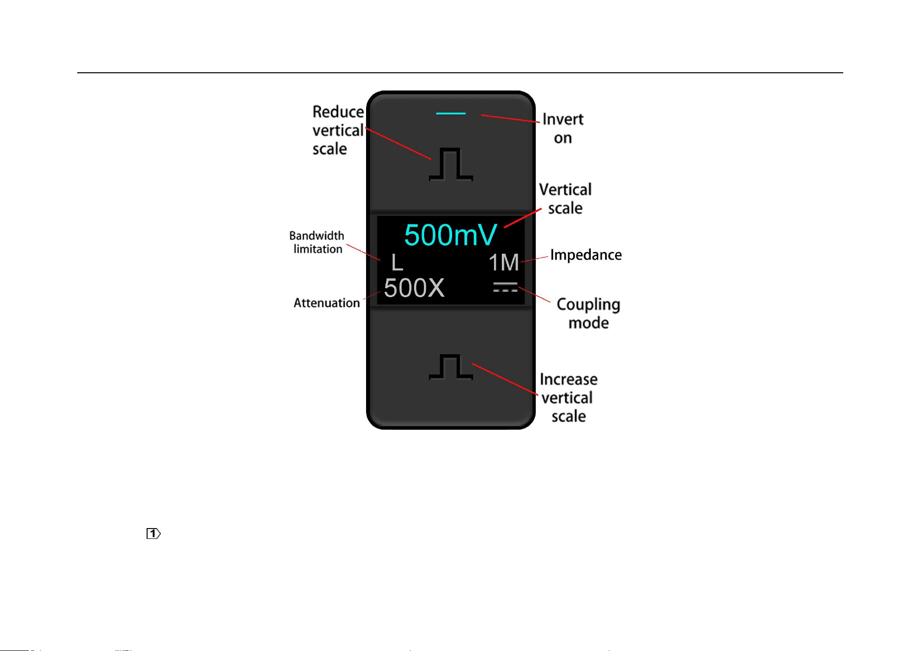
Chapter 5 Vertical System
159
Figure 5-3 Channel Display Interface
When CH1 is on, but the state is not the current channel, tap CH1 waveform or vertical sensitivity or channel
indicator or vertical sensitivity button or current channel selection button to set CH1 as the current channel, as
shown in Figure 5-4.
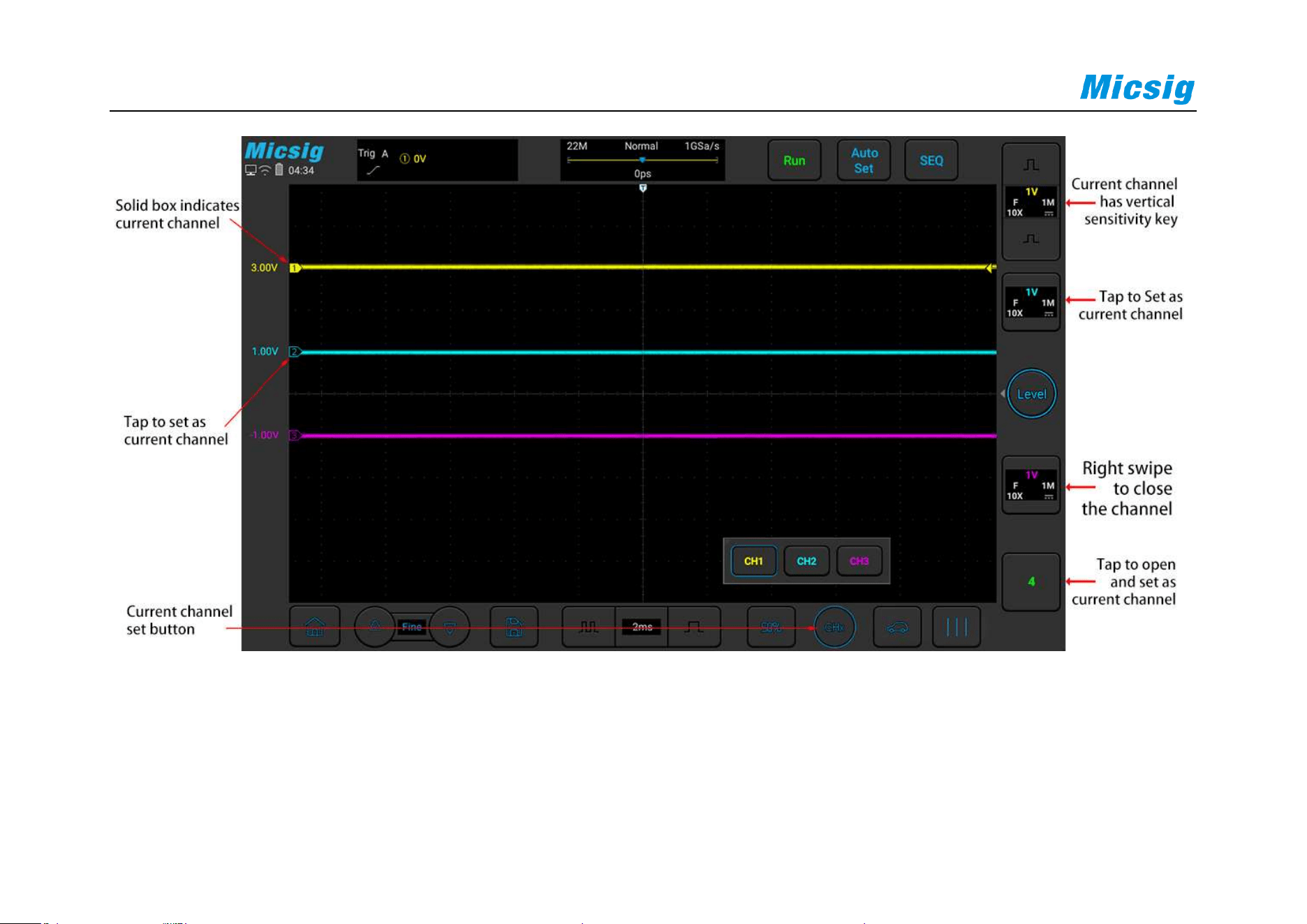
160
Figure 5-4 Channel Open, Close and Switching
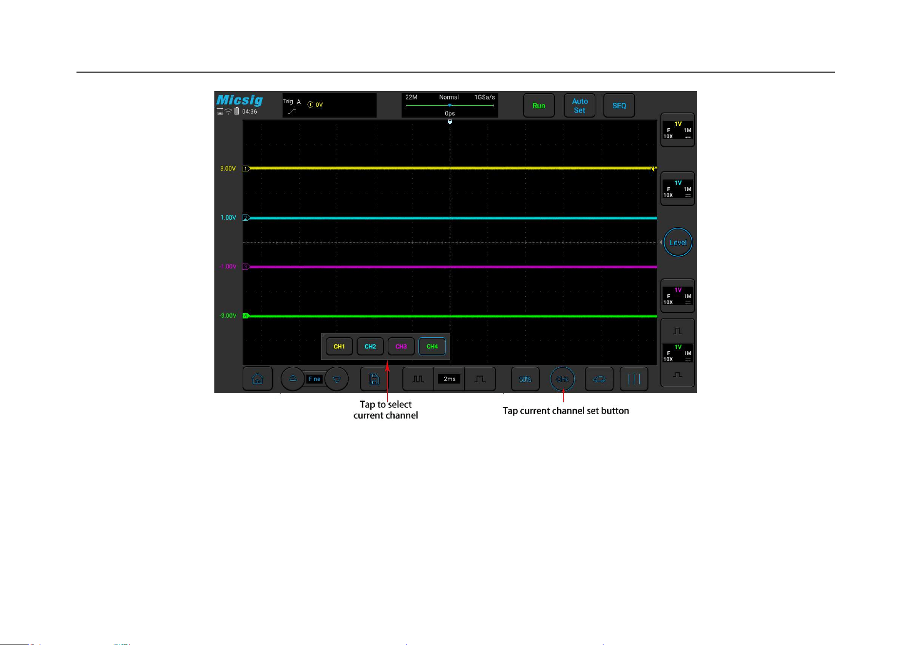
Chapter 5 Vertical System
161
Figure 5-5 Using the Current Channel Selection Button
Tap the current channel icon at the bottom of the screen to pop up the current channel switching menu and press the
button to light it up, as shown in Figure 5-5. Tap the button in the menu to switch the current channel. When this
function is opened:

162
a. the current channel may be switched in the channel switching menu;
b. the current channel menu can be moved anywhere on the screen;
c. only the open channel is displayed in the channel switching menu;
d. when the math or reference waveform is opened, the current channel switching menu is automatically opened.
5.2 Adjust Vertical Sensitivity
Tap the vertical sensitivity or buttons on the right side of the channel icon to adjust the vertical display
of the waveform corresponding to the channel, so that the waveform is displayed on the screen at an appropriate
size.
The vertical sensitivity scale (V/div) after each adjustment is displayed on the channel icon. For example,
means that the current vertical sensitivity of CH1 is 1.0V/div.

Chapter 5 Vertical System
163
The vertical sensitivity coefficient adjusts the vertical sensitivity of the analog channel in steps of 1-2-5 (the probe
attenuation coefficient is 1X), and the vertical sensitivity range of 1:1 probe is 1mV/div-10V/div (optionally
minimum at 500uV/div).
5.3 Adjust Vertical Position
The method of adjusting vertical position is as follows:
1) Coarse adjustment: In the waveform display area, hold the waveform and put one finger to slide up and down
for changing the vertical position of the waveform.
2) Fine adjustment: Click the fine adjustment button in the lower left corner of the screen to fine adjust the
vertical position of the waveform for the current channel.
5.4 Open Channel Menu
Right swipe the channel icon to open the desired channel menu.
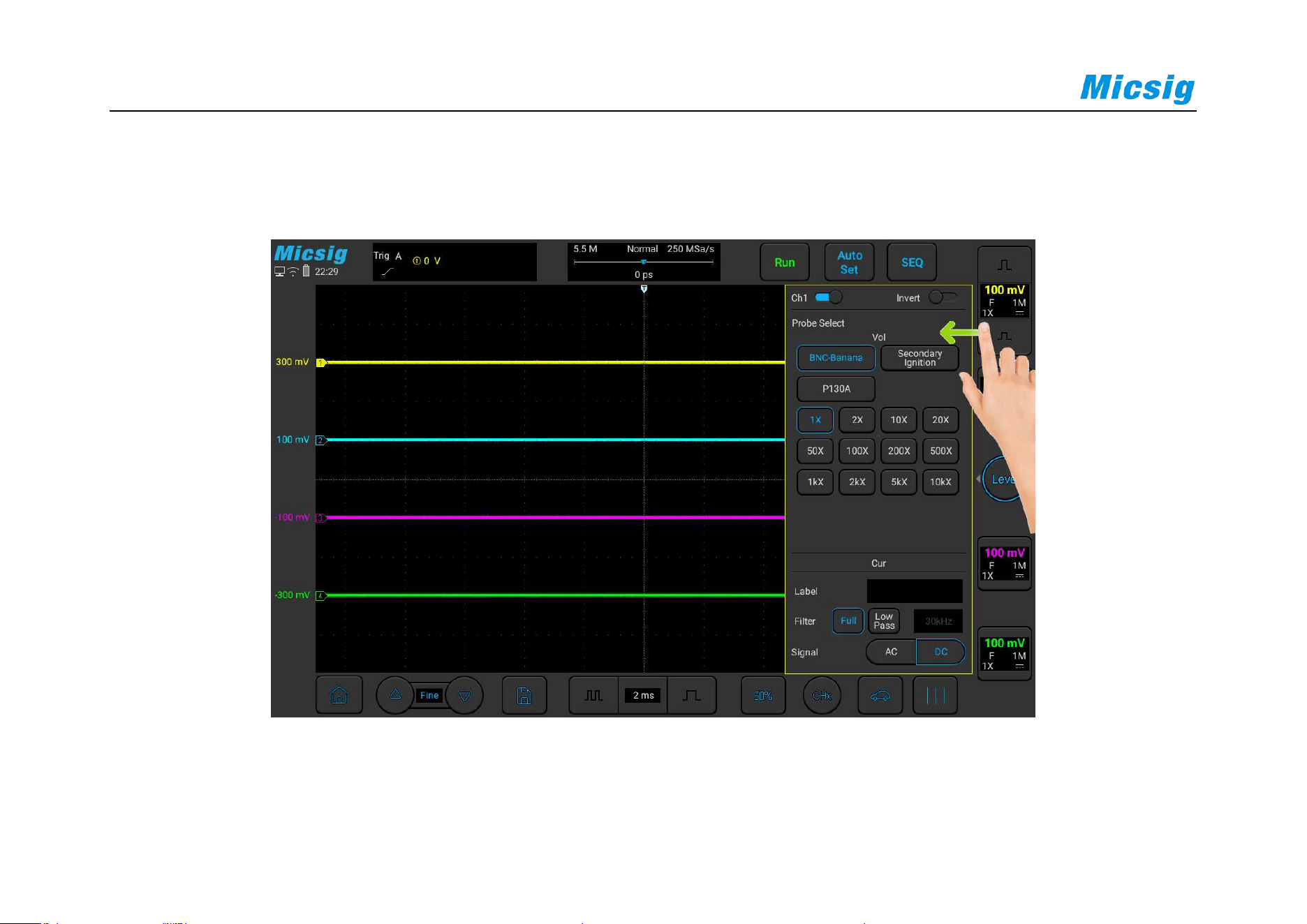
164
The channel menu is shown in Figure 5-6. Channel waveform inversion, channel bandwidth limit, probe type, probe
attenuation factor, channel coupling mode, channel on/off can be set in the vertical menu.
Figure 5-6 Channel menu

Chapter 5 Vertical System
165
5.4.1 Set Channel Coupling
Tap the icon under “Signal” and select “DC”, “AC” channel coupling modes in the pop-up box.
DC: DC coupling. Both the DC component and the AC component of the measured signal can pass, and can be
used to view waveforms as low as 0 Hz without large DC offset.
AC: AC coupling. Measured DC signal is blocked, and only the AC component can be allowed to pass, and used to
view waveforms with large DC offsets.
The oscilloscope is connected to the square wave signal with a frequency of 1KHz, an amplitude of 2V and an
offset of 1V. The waveforms of the channel couplings of DC, AC are shown in Figures 5-7, 5-8.
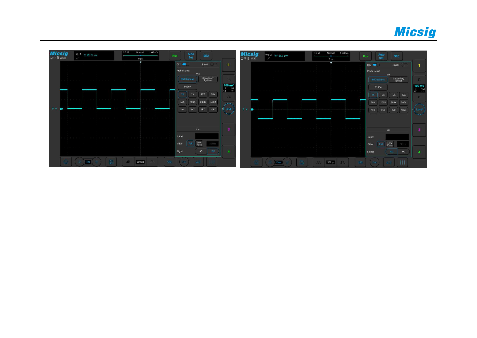
166
Figure 5-7 DC Coupling Figure 5-8 AC Coupling
Note: This setting is only valid for the current channel. To switch from the current channel, just tap the channel
icon, channel indicator icon or horizontal position pointed by the channel indicator icon for direct switching. You do
not need to exit the menu.

Chapter 5 Vertical System
167
5.4.2 Set Bandwidth Limit
Open the channel menu, find the “Bandwidth” selection box in the channel menu, set bandwidth limit, high-pass
filtering and low-pass filtering as needed.
Full Bandwidth: Allows signals of all frequencies to pass.
Low pass: Only signals below the currently set frequency upper limit are allowed to pass. (with the settings same
as High Pass)
Low-pass filtering can be set within the frequency range of 30kHz-100MHz.
The difference in bandwidth limitation can be visualized by the waveform. The full bandwidth is shown in Figure
5-9, the low pass is shown in Figure 5-10.
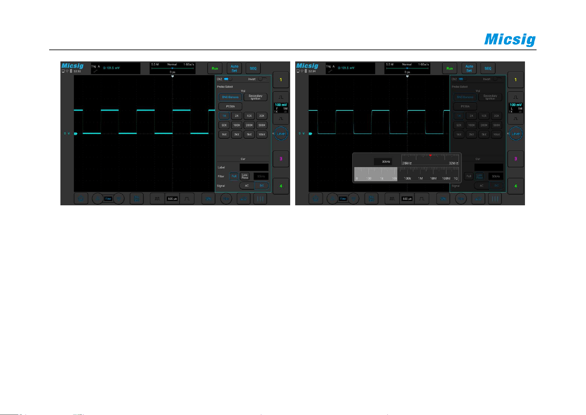
168
Figure 5-9 Full Bandwidth
Figure 5-10 Low Pass
5.4.3 Waveform Inversion
After selecting “Invert”, the voltage value of the displayed waveform is inverted. Inversion affects the way the
channel is displayed. When using a basic trigger, you need to adjust the trigger level to keep the waveform stable.
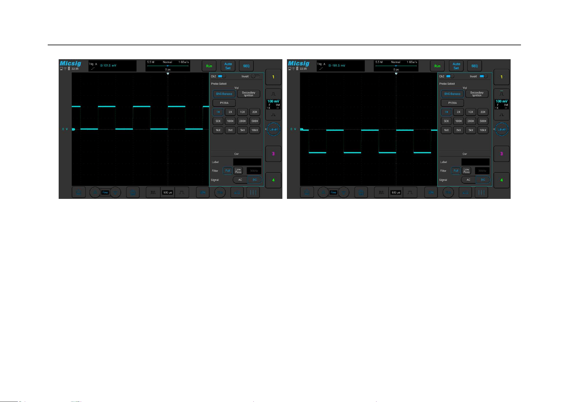
Chapter 5 Vertical System
169
Figure 5-11 Before Inversion Figure 5-12 After Inversion
5.4.4 Set Probe Type
Probe types are divided into voltage probe and current probe.
Probe type adjustment steps:
Open the channel menu, find the “Probe Type” checkbox in the channel menu, then select:

170
Vol - corresponding the voltage probe.
Cur - corresponding the current probe.
5.4.5 Set Probe Attenuation Coefficient
When measuring with a probe, the correct measurement result can only be obtained by setting the correct probe
attenuation ratio. In order to match the actual probe attenuation ratio, it is necessary to adjust the channel
attenuation factor correspondingly under the channel menu. When probe attenuation ratio is changed, the
corresponding attenuation ratio must be set on the channel menu to ensure the correctness of the waveform
amplitude and measurement result displayed by the oscilloscope.
Probe attenuation ratio and menu attenuation ratio are shown in the table below:

Chapter 5 Vertical System
171
Probe attenuation ratio / Menu attenuation ratio
1:1
1x
200:1
200x
2:1
2x
500:1
500x
10:1
10x
1000:1
1kx
20:1
20x
2000:1
2kx
50:1
50x
5000:1
5kx
100:1
100x
10000:1
10kx
Table 5-1 Probe Attenuation Ratio Correspondence Table
5.4.6 Labels
Labels can be added to each analog channel as needed, and the added label is displayed behind the channel
indicator.
Channel labels can be selected: none, custom, preset (including CAN_H, CAN_L, Flexray_H, Flexray_L).
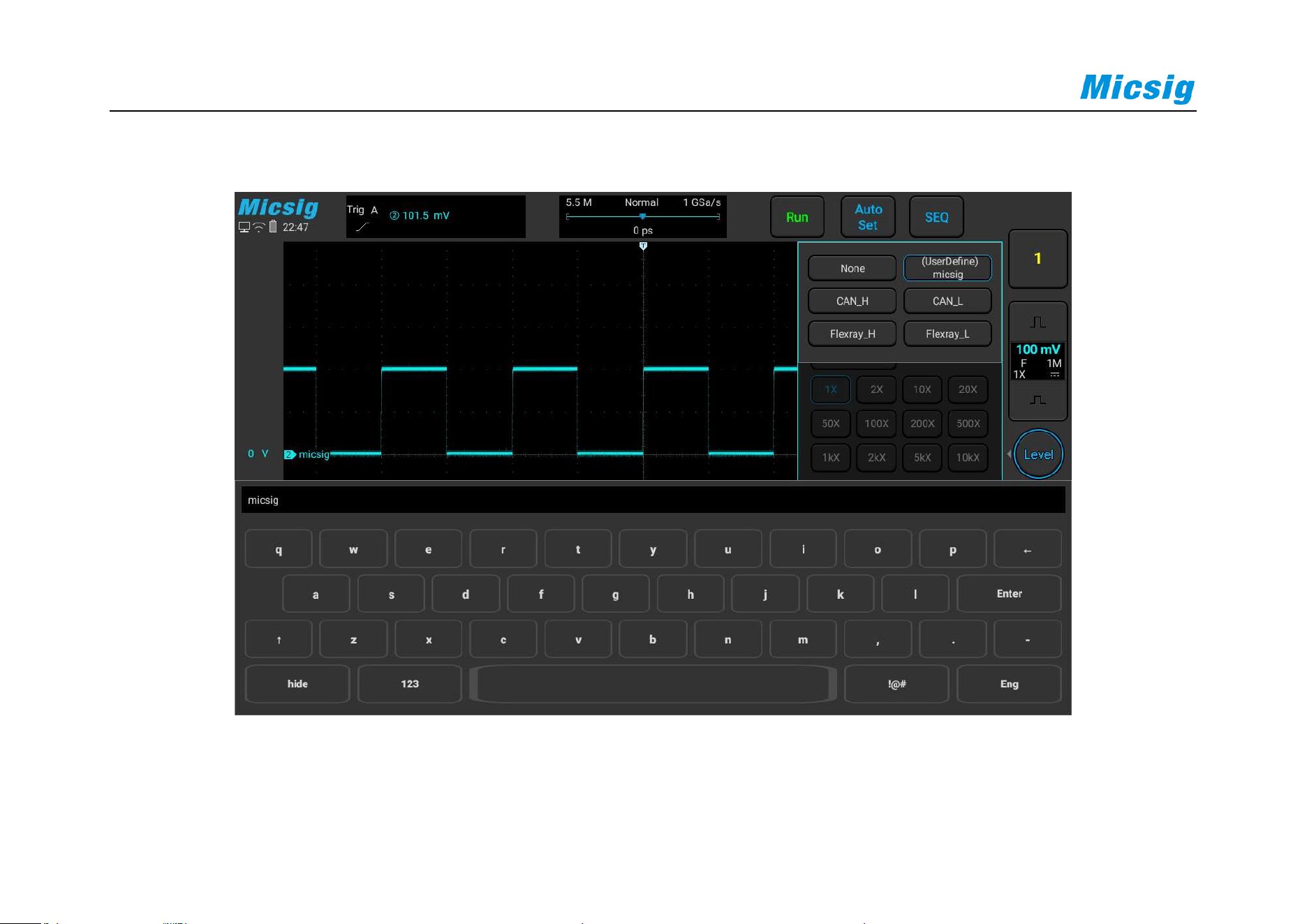
172
Figure 5-13 Label
Note: Customization supports up to 32 characters.

Chapter 6 Trigger System
173
Chapter 6 Trigger System
This chapter contains the detailed information of the trigger system of the oscilloscope. You are recommended to
read this chapter carefully to understand the set functions and operation of the trigger system of the ATO series
oscilloscope.
Trigger and trigger adjustment
Slope trigger
Edge trigger
Time out trigger
Pulse width trigger
Video trigger
Logic trigger
Serial bus trigger
Nth edge trigger
Runt trigger

174
6.1 Trigger and Trigger Adjustment
What is Trigger?
The oscilloscope can capture a waveform only when it meets a preset condition first. This action of capturing the
waveform according to the condition is Trigger. The so-called capture waveform is that the oscilloscope grabs a
signal and displays it. If it is not triggered, there is no waveform display.
What can Trigger be used for?
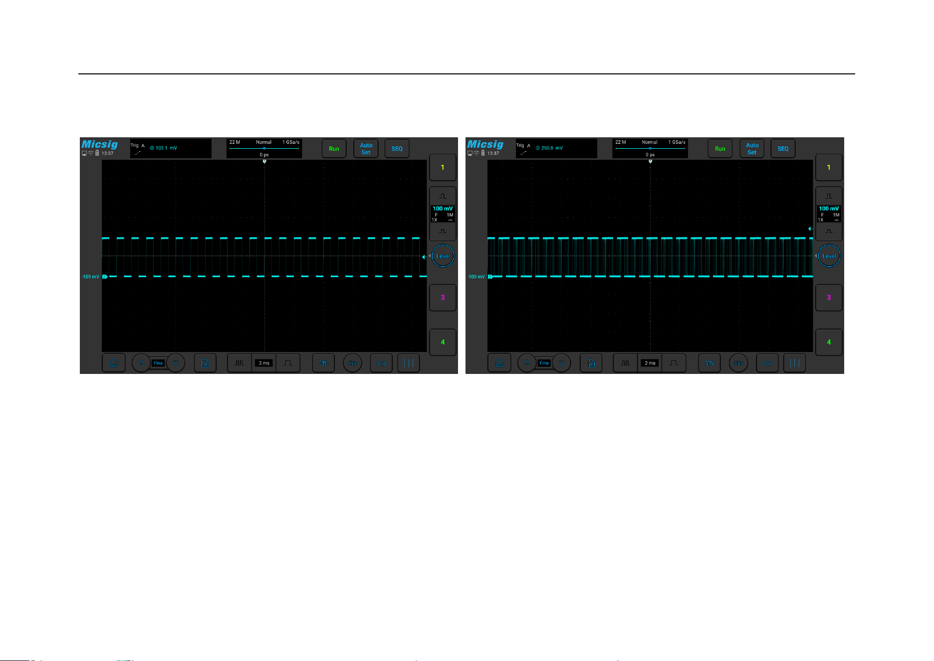
Chapter 6 Trigger System
175
(1) The oscilloscope can stably display a periodic signal.
Figure 6-1 Stably Displayed Periodic Signal Figure 6-2 Non-Stably Displayed Periodic Signal
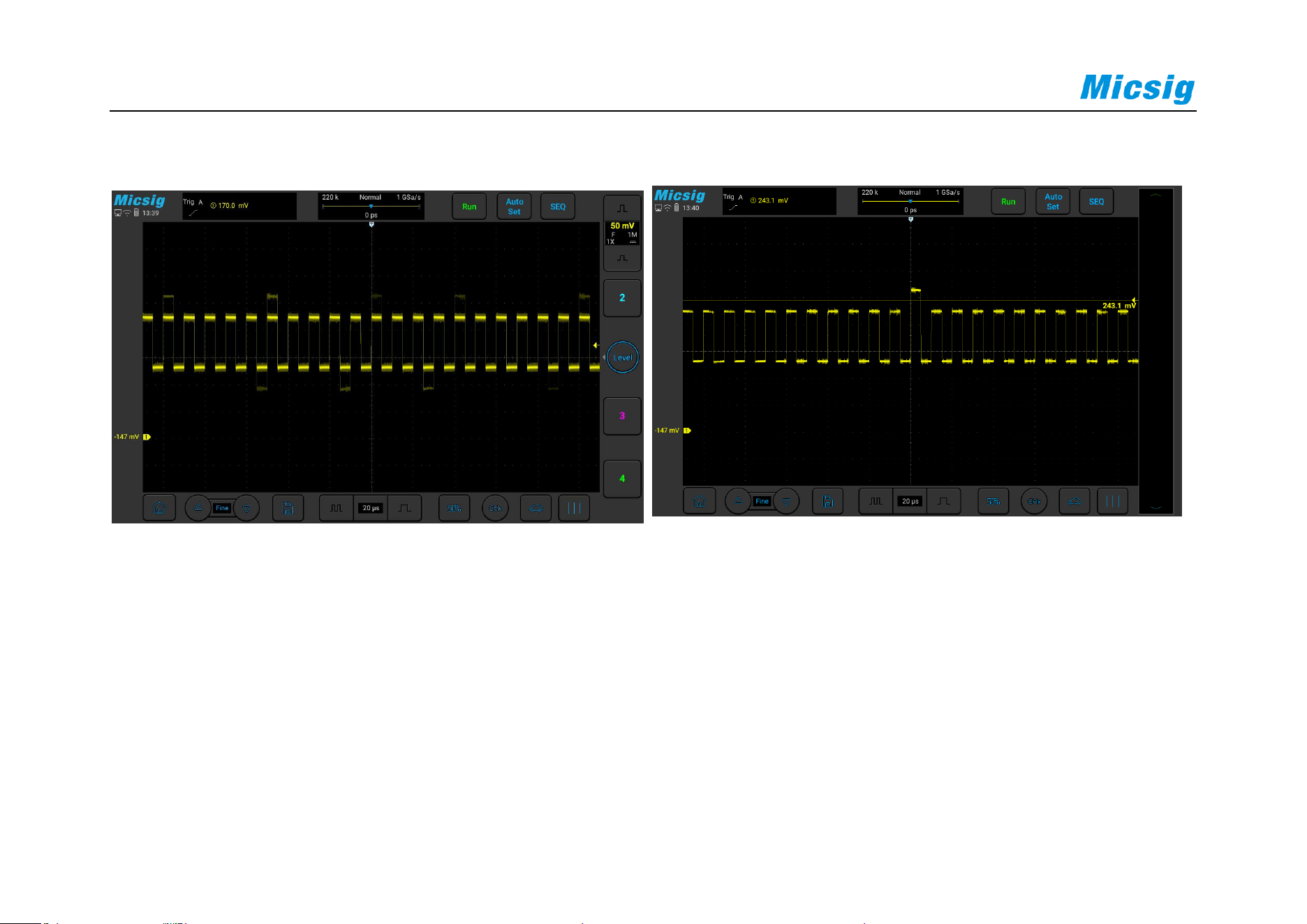
176
(2) Grab the segment you want to observe from a fast and complex signal
Figure 6-3 Abnormal Signal in Periodic Signals
Figure 6-4 Abnormal Signal Captured by Setting
Trigger Level

Chapter 6 Trigger System
177
What is Forced Trigger?
When the oscilloscope does not meet the trigger condition, the artificial or automatic oscilloscope trigger is the
forced trigger. It means that the oscilloscope only grabs a signal segment for display regardless of whether the
condition is met or not.
Automatic forced trigger is set in the menu. In the trigger settings, there is usually a trigger mode option, which can
be set as “Normal” or “Auto”. Normal trigger means trigger after meeting the set condition. Automatic trigger is a
kind of forced trigger. The oscilloscope will be force triggered if it does not trigger for a certain period of time.
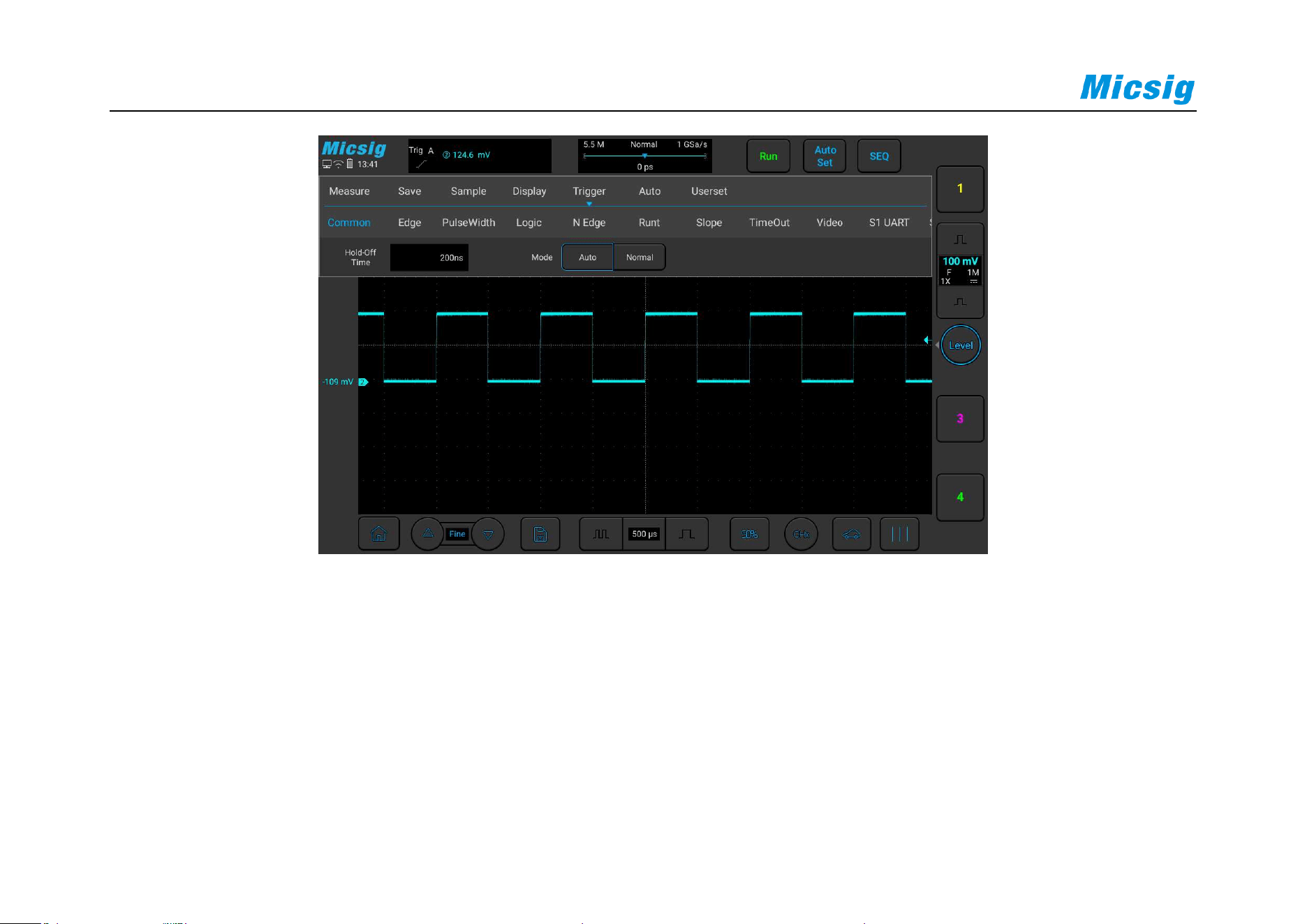
178
Figure 6-5 Oscilloscope Trigger Mode Setting
If a signal feature is not understood, the oscilloscope should be set as “Auto” mode, which can ensure that the
oscilloscope can also display the waveform when other trigger settings are not correct. Although the waveform is
not necessarily stable, it can provide the intuitive judgment for our further adjustment of the oscilloscope. The
signal in Figure 2-10 is the result of forced trigger in “Auto” mode.
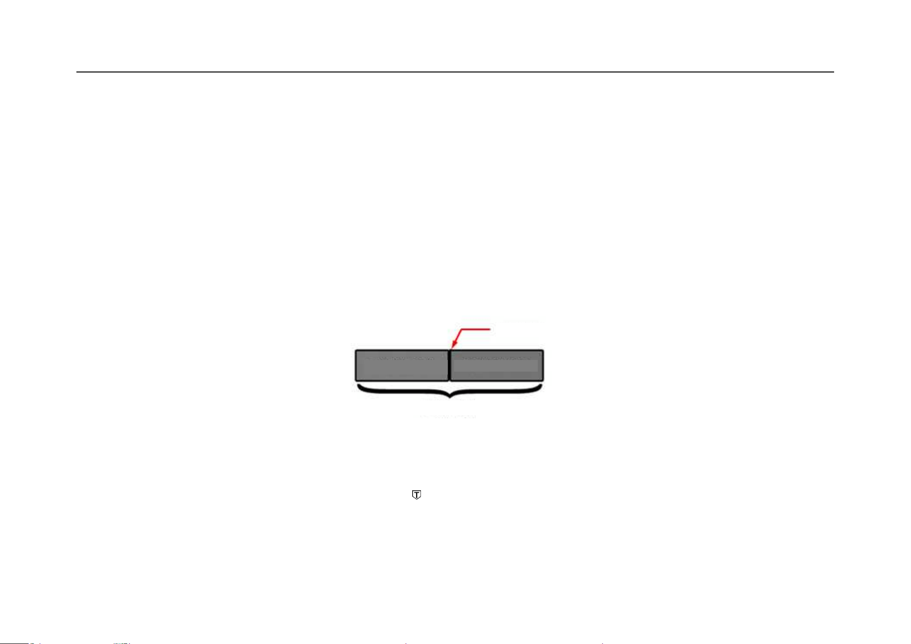
Chapter 6 Trigger System
179
When we set a specific trigger condition for a specific signal, especially when the time interval for satisfying the
trigger condition is long, we need to set the trigger mode to “Normal” so as to prevent the oscilloscope from
automatic forced trigger.
Figure 6-6 shows a conceptual demonstration of the acquisition memory. In order to understand the trigger event,
the acquisition memory can be divided into pre-trigger and post-trigger buffers. The position of the trigger event in
the acquisition memory is defined by the time reference point and trigger position (horizontal delay) settings.
Figure 6-6 Conceptual Demonstration of Acquisition Memory
All events displayed to the left of the trigger point occur before trigger. These events are called pre-trigger
messages that show events before the trigger point. All events to the right of the trigger point is called post-trigger
Trigger Event
Acquisition Memory
Pre-trigger Buffer
Post-trigger Buffer
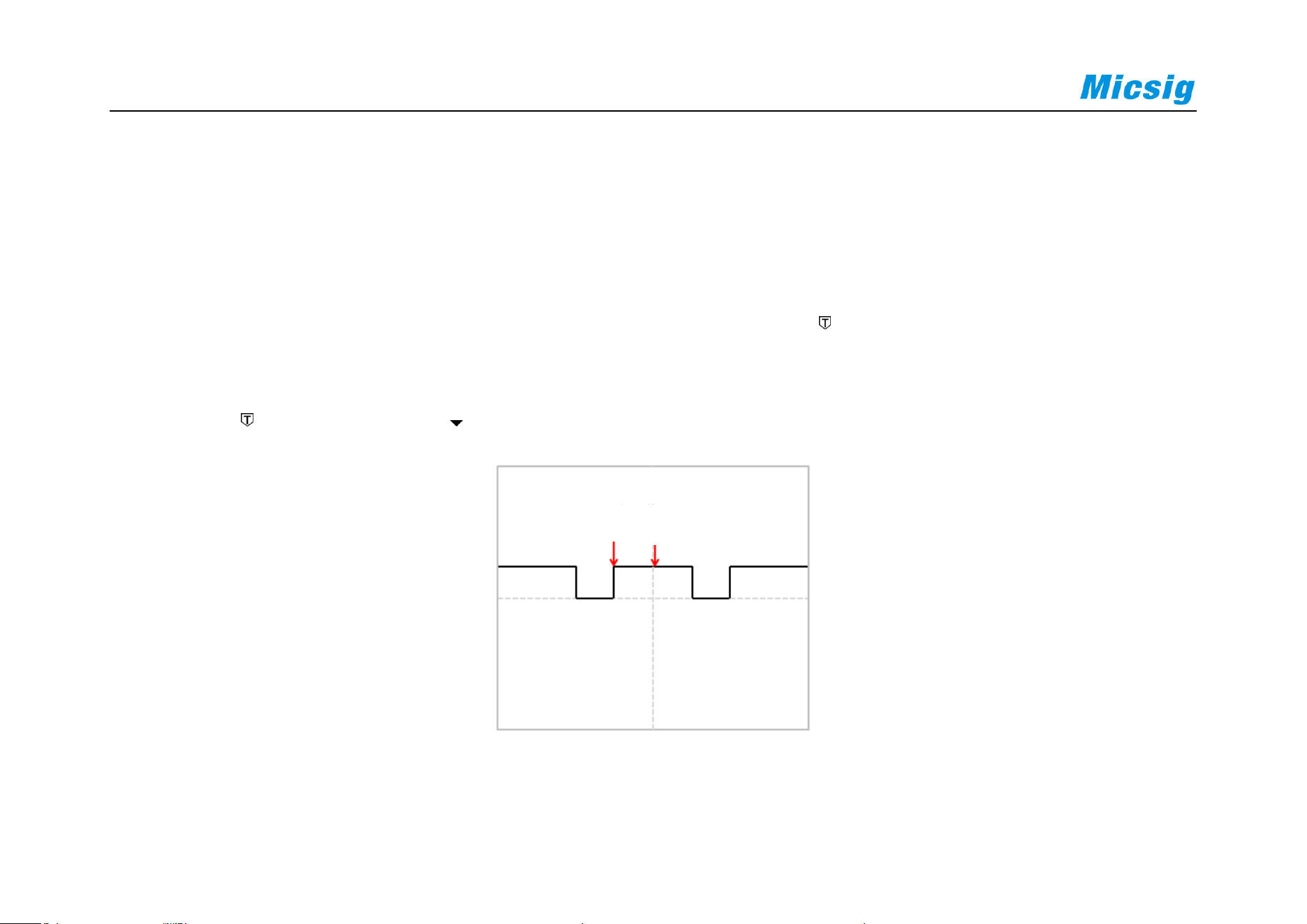
180
messages. The number of delay ranges available (pre-trigger and post-trigger messages) depends on the selected
time base and memory depth.
Adjust trigger position (horizontal delay)
Fingers swipe left and right in the waveform display area, the trigger point will move horizontally, the horizontal
delay time changes, and the delay time is displayed at the top center of the screen, that is, the distance between the
trigger point and the center line of the waveform display area is displayed.
Figure 6-7 Horizontal Delay
Horizontal Delay
Trigger
Center Position

Chapter 6 Trigger System
181
When the trigger point is located on the left side to the center line of the waveform display area, the delay
time is displayed as a positive value; When the trigger point is located on the right side to the time reference
point , and the delay time is displayed as a negative value; the trigger point overlaps with the center line of
the waveform display area, and the delay time is zero.
Trigger level
Trigger level is the signal voltage corresponding to the set trigger point. When the trigger level is changed, a
horizontal line will appear temporarily on the screen to tell you the level position (the specific value of the trigger
level is displayed in the upper right corner of the screen), then the horizontal line disappears, the trigger level is
indicated by a small arrow and the indication icon can be dragged to adjust the trigger level value. The trigger
level is shown in Figure 6-8 (the arrow indicates the trigger level line).
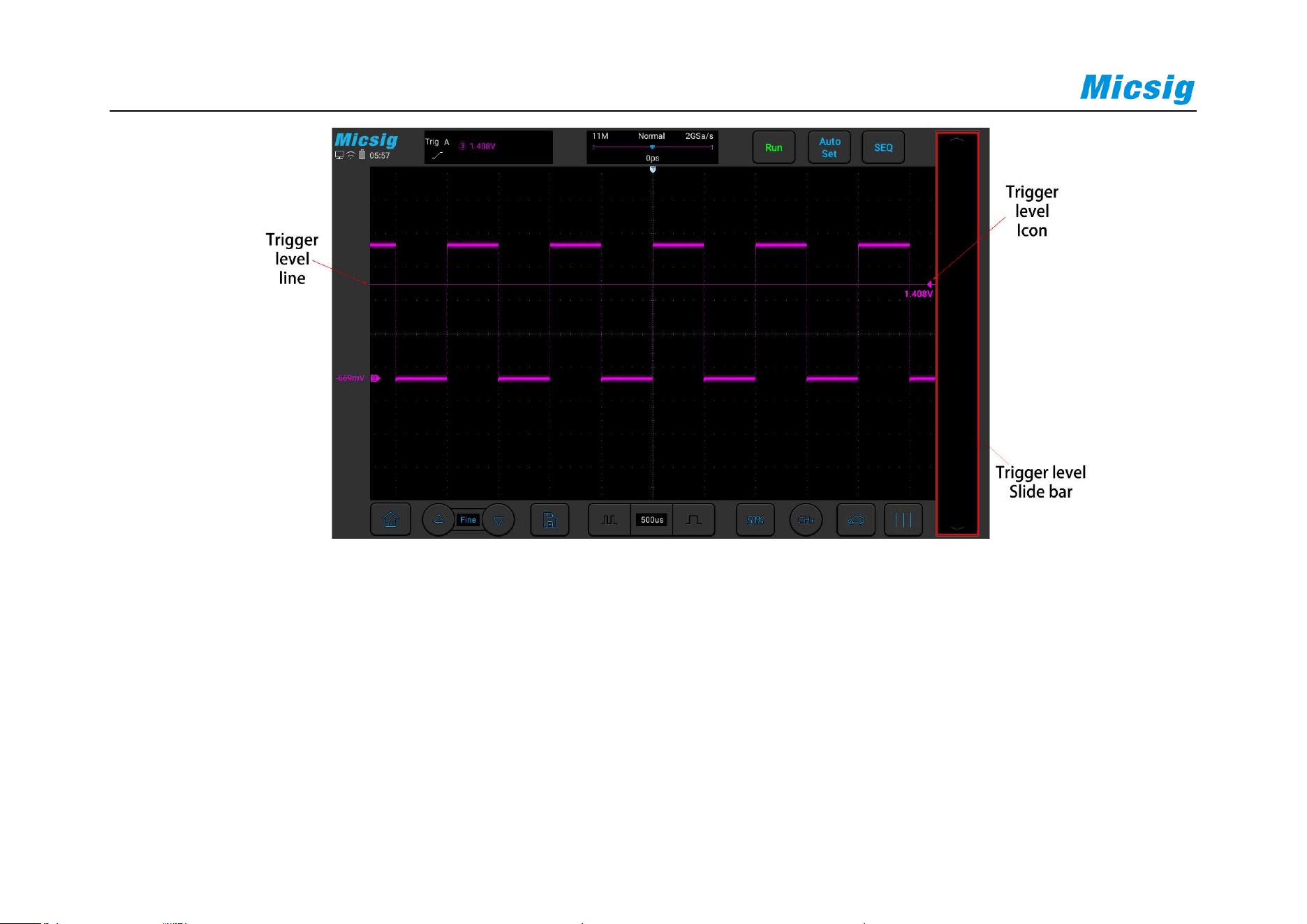
182
Figure 6-8 Trigger Level
Adjust trigger level
The trigger level can be coarsely adjusted and finely adjusted.
Coarse adjustment: Slide up and down in the trigger level adjustment area.
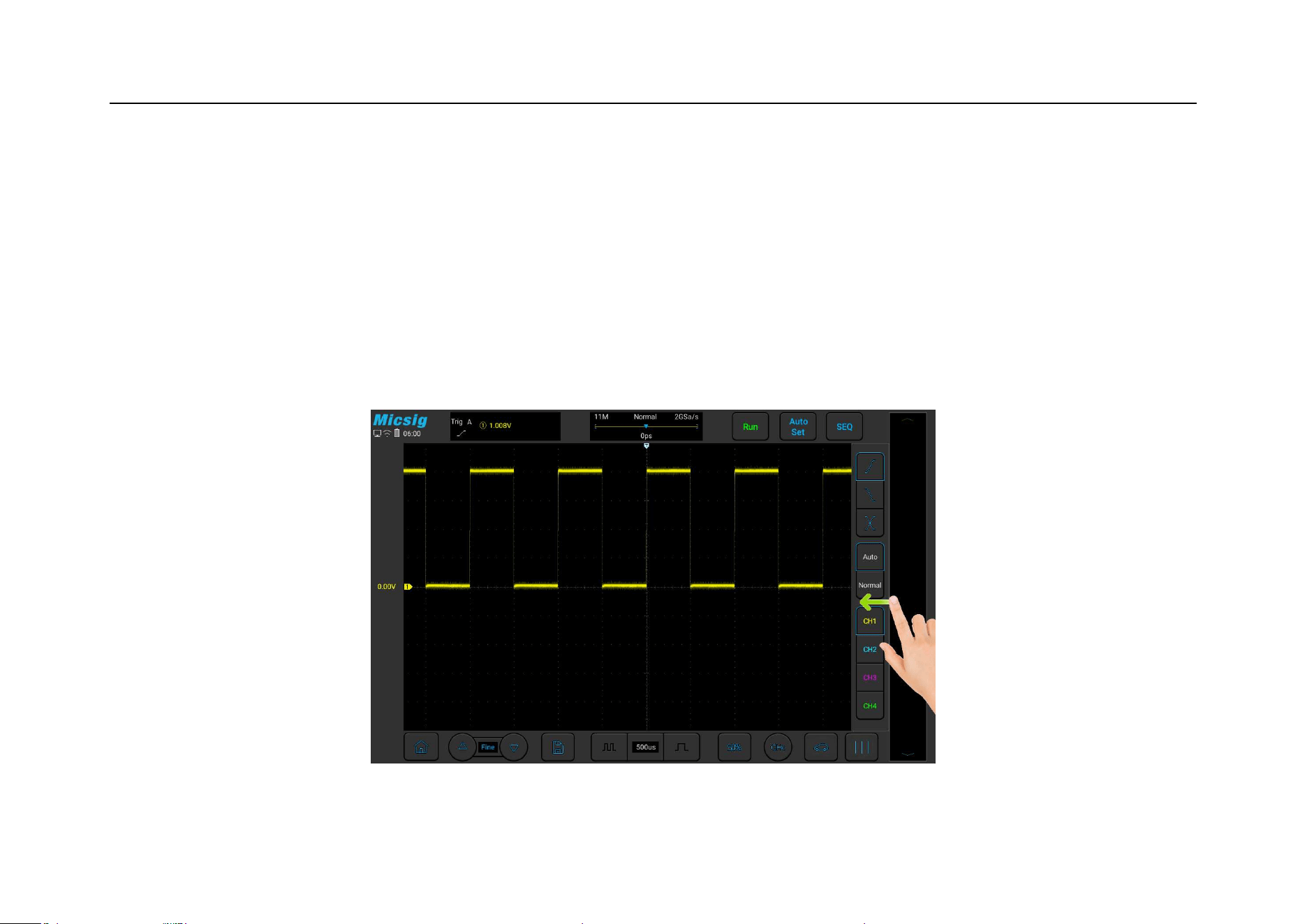
Chapter 6 Trigger System
183
Fine adjustment: Tap the fine adjustment button in the lower left corner of the screen for fine adjustment of the
trigger level.
Trigger setting shortcut
Left swipe from trigger level slide bar to open trigger setting shortcut, which includes trigger source, trigger mode
etc.
Figure 6-9 Trigger setting shortcut
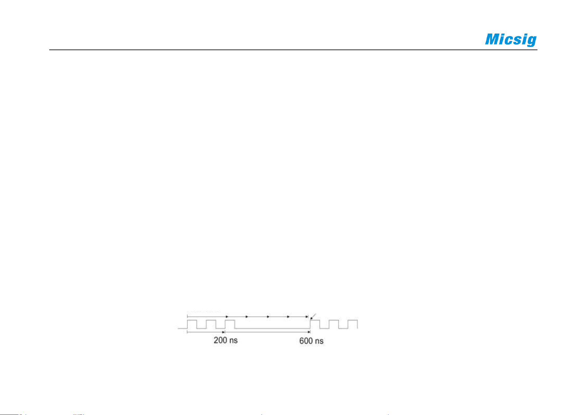
184
Set trigger hold-off time
The trigger hold-off time can set up the waiting time of the oscilloscope after the trigger and before the trigger
circuit is reconnected. During hold-off time, the oscilloscope does not re-trigger until the end of the hold-off time,
and the hold-off time can be used to stably trigger complex waveforms. The trigger hold-off time ranges from
200ns~10s.
The hold-off may be used to trigger on repetitive waveforms with multiple edges (or other events) between
waveform repetitions. If the shortest time between triggers is known, the hold-off may also be used to trigger on the
first edge.
For example, to obtain stable trigger on the repetitive pulse trigger shown below, set the hold-off time to a
value >200ns but <600ns.
Figure 6-10 Trigger Hold-Off Time
Hold-off Time
Oscilloscope Trigger Position
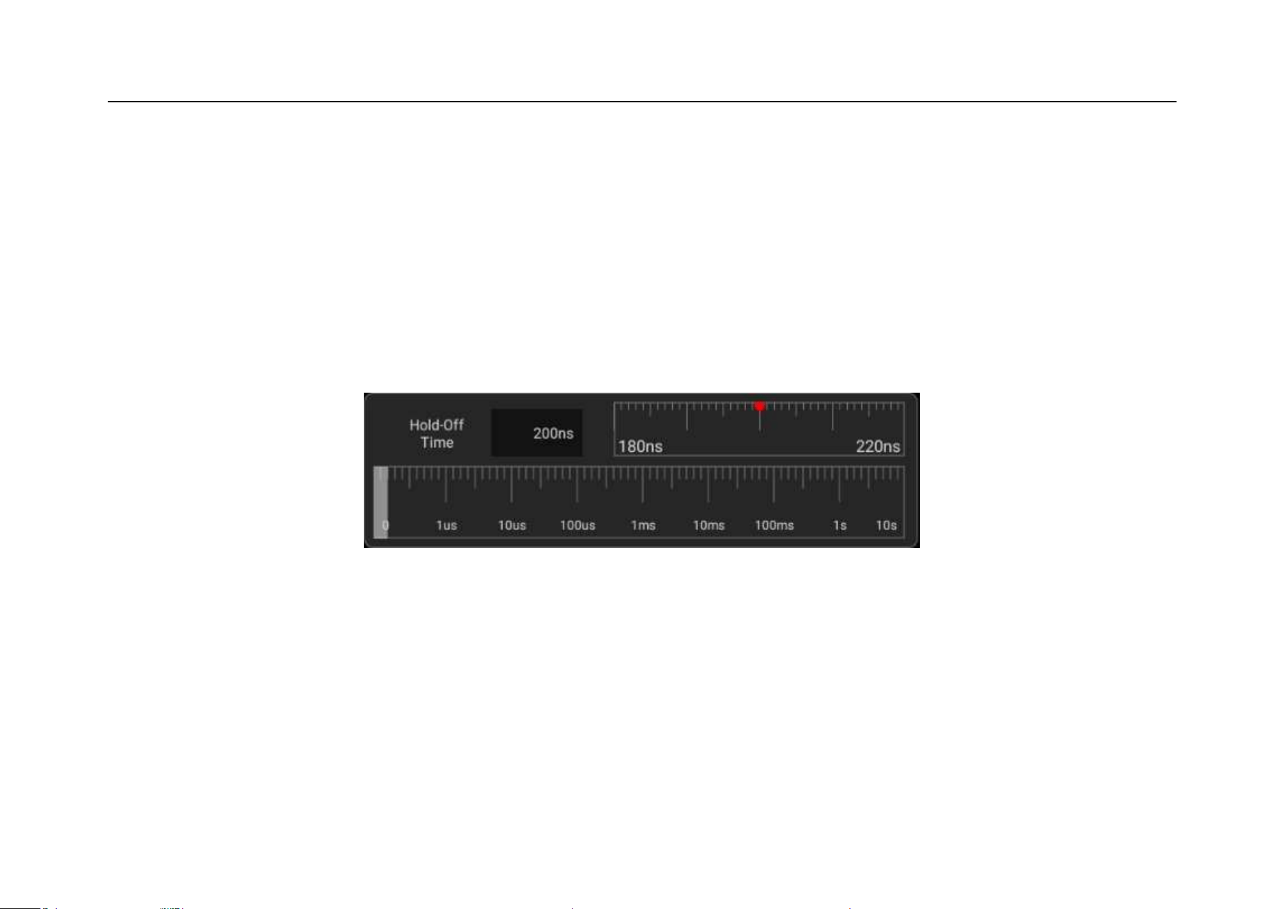
Chapter 6 Trigger System
185
Set trigger hold-off time:
1) Tap “Trigger” on the main menu to open the trigger menu. Under “Common”, tap the box after “Rejection
Time” to open the hold-off time adjustment interface. The trigger time is displayed on the upper left, the fine
adjustment time scale is displayed on the upper right, and the coarse time scale is displayed below, as shown in
Figure 6-11.
Figure 6-11 Trigger Hold-Off Time Set Interface
2) When adjusting the time, drag or tap the coarse adjustment scale for coarse adjustment, and then drag the fine
adjustment scale for fine adjustment of the hold-off time.
Trigger hold-off operation prompt

186
It is typically used for complex waveforms. The correct rejection setting is usually slightly smaller than one
repetition of the waveform. Setting the hold-off time to this time can become the only trigger point for the repetitive
waveform.
Changing the time base setting will not affect the trigger hold-off time.
Using Zoom function, you can tap “Run/Stop” to stop, then horizontally move and zoom the data to find the
position where the waveform is repeated. Use the cursor to measure this time and then set the hold-off time.
Use “SEQ” button for single acquisition
Usually when performing a single acquisition, you must initiate some operations on the measured equipment, and
the oscilloscope is not desired to trigger automatically before these operations. The trigger condition indicator
is displayed in the upper left corner of the screen before starting operations in the circuit (this means the pre-trigger
buffer is filled).

Chapter 6 Trigger System
187
6.2 Edge Trigger
When the edge of trigger signal reaches a certain trigger level, the set signal is triggered and generated. Trigger
occurs on either edge of the rising edge (indicating icon at the top of the screen), falling edge ( ) or dual edge
( ), and the trigger level can be set to change the vertical position of the trigger point on the trigger edge, namely
the intersection point of the trigger level line and the signal edge. The stable waveform can be obtained by correctly
setting the edge trigger coupling mode. Edge trigger menu is shown in the table below:
Trigger Option
Setting
Description
Trigger Source
CH1
Set CH1 as trigger signal source
CH2
Set CH2 as trigger signal source
CH3
Set CH3 as trigger signal source
CH4
Set CH4 as trigger signal source

188
Slope
Rising edge
Set signal trigger on the rising edge
Falling edge
Set signal trigger on the falling edge
Dual edge
Set signal trigger on either rising edge or falling edge
Coupling
DC
AC and DC components getting through trigger signals
AC
Filter out the DC component of trigger signals
HF rejection
Suppress signals above 50KHz in trigger signals
LF rejection
Suppresses signals below 50KHz in trigger signals
Noise rejection
Low-sensitivity DC coupling to suppress high-frequency noise
in trigger signals
Set CH1 rising edge trigger and coupling as DC with operation steps as follows:
1) Tap “Trigger” on the main menu to open the trigger menu, select edge trigger in the trigger type, and set edge
trigger as follows, as shown in Figure 6-12:
Trigger source: CH1;
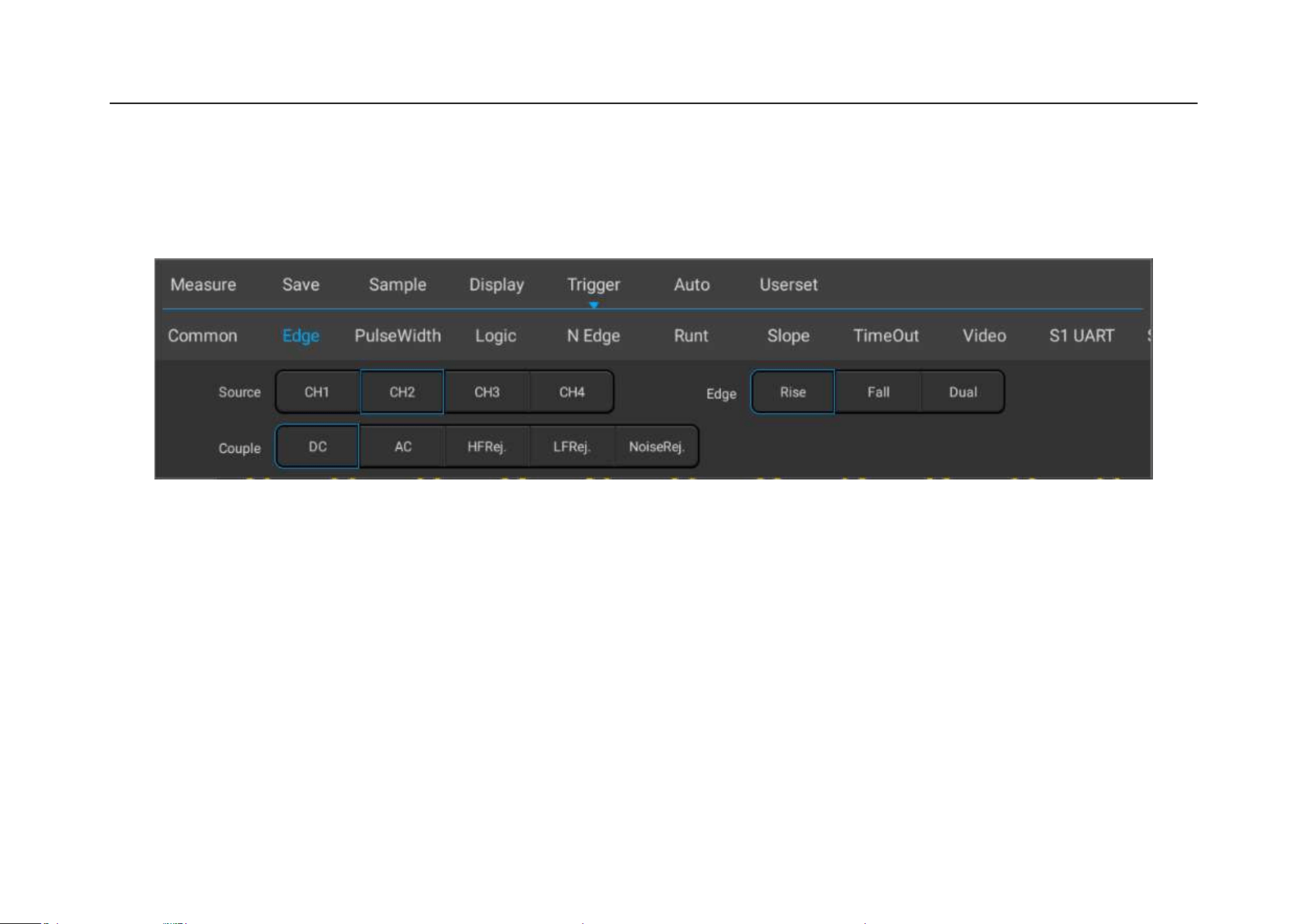
Chapter 6 Trigger System
189
Trigger coupling mode: DC;
Trigger edge: rising.
Figure 6-12 Edge Trigger Setting Menu
2) Adjust the trigger level to ensure that the waveform can be triggered stably, for example, the trigger level is set
to 1V.
Trigger coupling description
When the edge trigger setup menu is opened, the trigger coupling option is displayed below the menu. Trigger
coupling includes DC, AC, HFRei., LFRej., NoiseRej, see Figure 6-13:
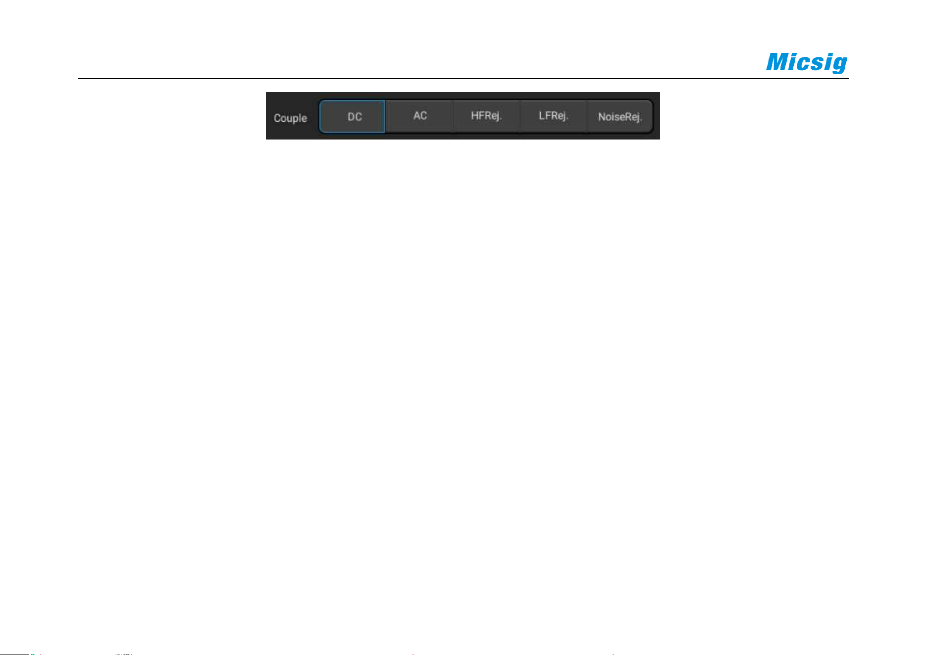
190
Figure 6-13 Trigger Coupling Menu
1) DC coupling - allows DC and AC signals to enter the trigger path.
2) AC coupling - removes any DC offset voltage from the trigger waveform.
When the waveform has a large DC offset, stable edge triggering can be achieved using AC coupling.
3) HFRej. (High Frequency Rejection Coupling) - removes high frequency components from the trigger
waveform, using high frequency rejection to remove high frequency noises or noises from fast system clocks,
from trigger paths such as AM or FM radio stations.
4) LFRej. (Low Frequency Rejection Coupling) - removes any unnecessary low frequency components from the
trigger waveform, for example, power line frequencies that can interfere with correct trigger.

Chapter 6 Trigger System
191
When there is low frequency noise in the waveform, stable edge triggering can be obtained using LF rejection
coupling.
5) NoiseRej. (Noise Rejection Coupling) - Noise rejection can add extra hysteresis to the trigger circuit. By
increasing the trigger hysteresis band, the possibility of noise triggering can be reduced. But it also reduces the
trigger sensitivity, so triggering the oscilloscope requires a slightly larger signal.
Note: Trigger coupling is independent of channel coupling.
6.3 Pulse Width Trigger
The trigger happens when the trigger signal pulse width (8ns~10s, the trigger type indication icon at the top of the
screen is ) reaches the set condition and the signal voltage reaches the set trigger level. Pulse width trigger
menu is shown in the following table:
Trigger Option
Setting
Description
Trigger Source
CH1
Set CH1 as trigger signal source

192
Trigger Option
Setting
Description
CH2
Set CH2 as trigger signal source
CH3
Set CH3 as trigger signal source
CH4
Set CH4 as trigger signal source
Polarity
Positive
Trigger on setting the positive pulse width of signals
Negative
Trigger on setting the negative pulse width of signals
Trigger Condition
<T
Trigger when the signal pulse width is smaller than pulse width T
>T
Trigger when the signal pulse width is greater than pulse width T
=T
Trigger when the signal pulse width is equal to pulse width T
≠T
Trigger when the signal pulse width is not equal to pulse width T
Trigger Pulse
Width
8ns~10s
Set the trigger pulse width
Notes: Conditions of greater than, smaller than, equal to or not equal to indicating that the error is 6%.

Chapter 6 Trigger System
193
Trigger steps of positive polarity pulse width: (taking CH1 as an example)
1) Tap “Trigger” on the main menu to open the trigger menu, select the pulse width trigger in the trigger type, and
set the pulse width trigger as follows, as shown in Figure 6-14:
Trigger source: CH1;
Trigger pulse polarity: positive;
Trigger level: 1V
Trigger condition and pulse width time: “greater than”, the adjustment time is 180us.
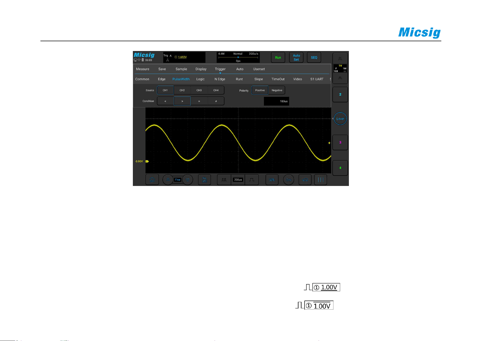
194
Figure 6-14 Pulse Width Trigger Setting Menu
Pulse width trigger setting description:
1) Pulse polarity selection
The selected pulse polarity icon is displayed in the upper right corner of the display screen. The positive pulse
is higher than current trigger level (CH1 positive pulse indication icon ), and the negative pulse is
lower than current trigger level (CH1 negative pulse indication icon ). When triggered on positive
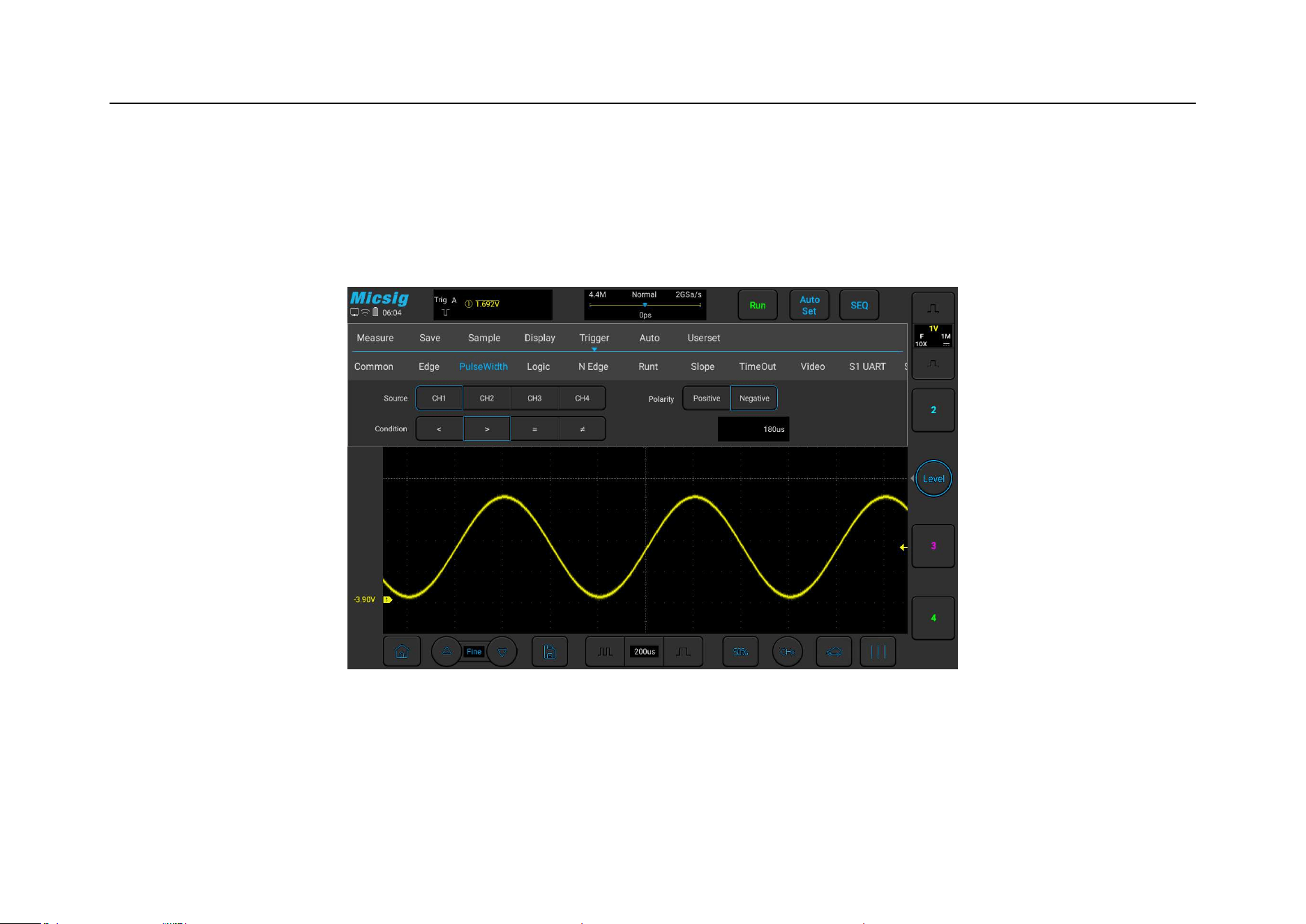
Chapter 6 Trigger System
195
polarity pulse, if the restrictions are true, the trigger will happen on the high-to-low transition of the pulse;
when triggered on negative polarity pulse, if the restrictions are true, the trigger will happen on the low-to-high
transition. (Figure 6-15 Negative Pulse Level Flip)
Figure 6-15 Negative Polarity Pulse Level Flip
2) Trigger condition and pulse width time setting
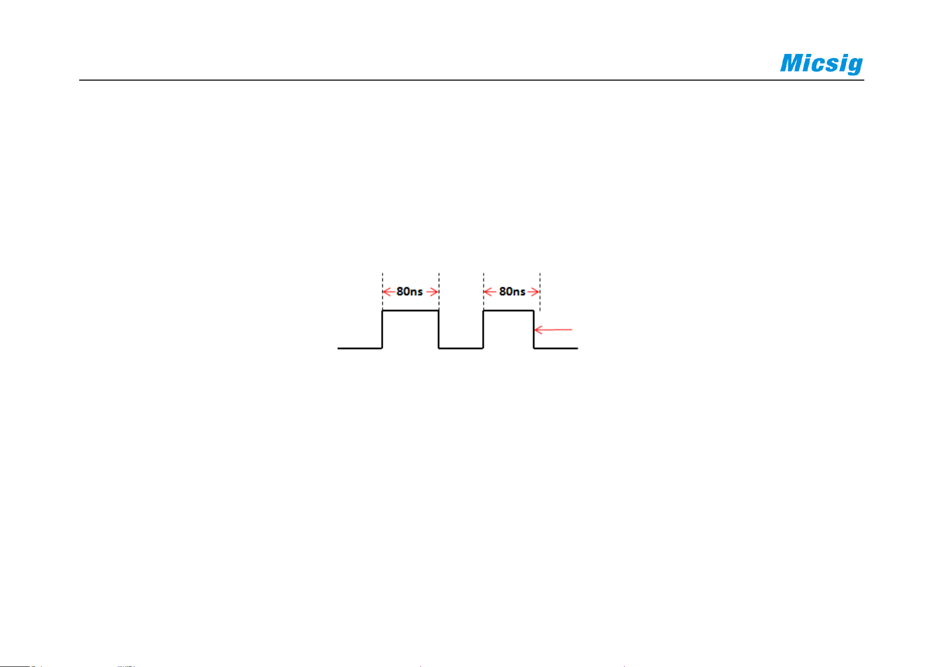
196
Time restrictions that can set in the trigger condition: <, >, =, ≠.
Smaller than the time value (<)
For example, for positive pulse, if it is set as T<80ns, the trigger will happen stably only when the pulse
width is smaller than 80ns (Figure 6-16 Trigger Time T<80ns).
Figure 6-16 Trigger Time T<80ns
Greater than the time value (>)
For example, for positive pulse, if it is set as T>80ns, the trigger will happen stably only when the pulse
width is greater than 80ns (Figure 6-17 Trigger Time T>80ns).
Trigger
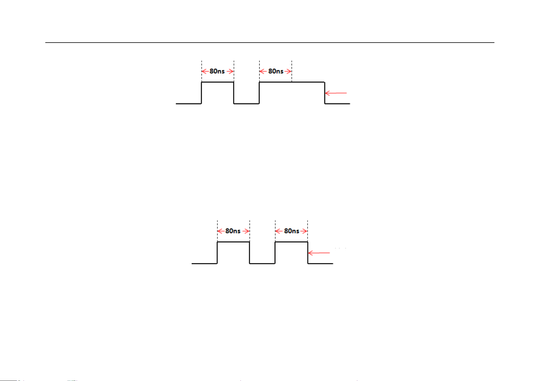
Chapter 6 Trigger System
197
Figure 6-17 Trigger Time T>80ns
Equal to the time value (=)
For example, for positive pulse, if it is set as T=80ns, the trigger will happen stably only when the pulse
width is equal to 80ns (Figure 6-18 Trigger Time T=80ns).
Figure 6-18 Trigger Time T=80ns
Not equal to the time value (≠)
Trigger
Trigger
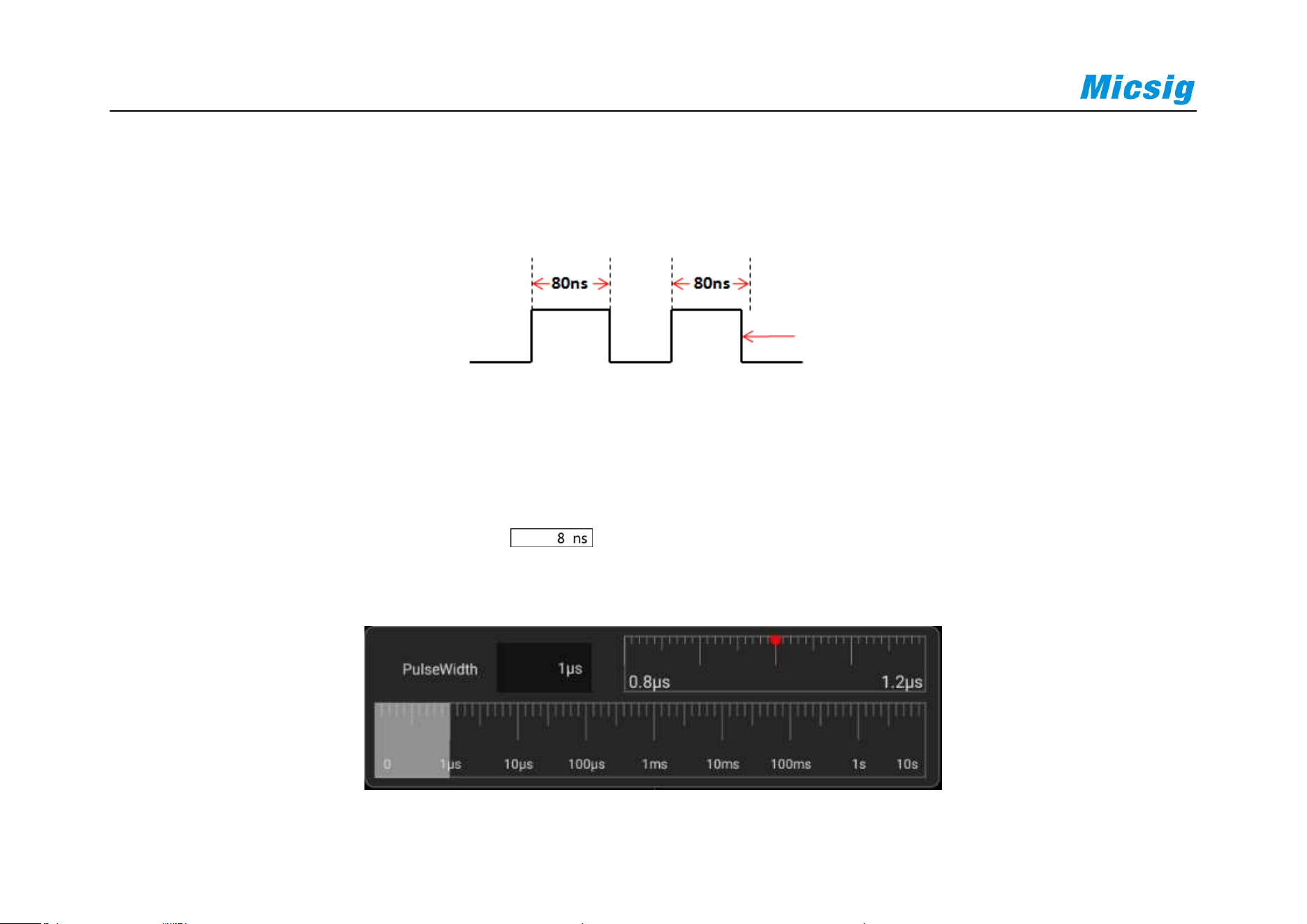
198
For example, for positive pulse, if it is set as T≠80ns, the trigger will happen stably only when the pulse
width is not equal to 80ns (Figure 6-19 Trigger Time T≠80ns).
Figure 6-19 Trigger Time T≠80ns
The trigger pulse width time can be set as 8ns~10s.
Tap the pulse width time setting box to pop up the time adjustment interface (as shown in Figure 6-
20), and adjust the pulse width time. Adjust the pulse width time by adjusting or dragging the time scale.
Figure 6-20 Pulse Width Time Adjustment Interface
Trigger

Chapter 6 Trigger System
199
6.4 Logic Trigger
Trigger happens when the level between analog channels satisfies a certain logical operation (AND, OR, NAND,
NOR) and the signal voltage reaches the set trigger level and the trigger logic width (8ns~10s). Logic trigger menu
descriptions are shown in the table below:
Trigger Option
Setting
Description
Trigger Source
CH1
High
Set CH1 as high
Low
Set CH1 as low
None
Set CH1 as none
CH2
High
Set CH2 as high
Low
Set CH2 as low
None
Set CH2 as none
CH3
High
Set CH3 as high

200
Low
Set CH3 as low
None
Set CH3 as none
CH4
High
Set CH4 as high
Low
Set CH4 as low
None
Set CH4 as none
Trigger Logic
AND
Select the logic of trigger source as “AND”
OR
Select the logic of trigger source as “OR”
NAND
Select the logic of trigger source as “NAND”
NOR
Select the logic of trigger source as “NOR”
Trigger
Condition
Change to true value
Trigger when the logic changes to true value
Change to false value
Trigger when the logic changes to false value
<, >, =, ≠T
If logic status for hold time as <, >, =, ≠T, then trigger
Logic Time
8ns~10ns
Set trigger logic time

Chapter 6 Trigger System
201
Notes: Conditions of greater than, smaller than, equal to or not equal to indicating that the error is 6%.
Logic trigger operation steps between channels:
1) Tap “Trigger” on the main menu to open the trigger menu, select logic trigger in the trigger type, and set the
logic trigger as follows, as shown in Figure 6-21:
Logic levels: CH1, CH3: High; CH2, CH4: Low; (without reference to the channel of logic operation, the
level selection is None to avoid interference to the logic operation);
Logic gate: AND;
Condition: <;
Logic time: 400ns.
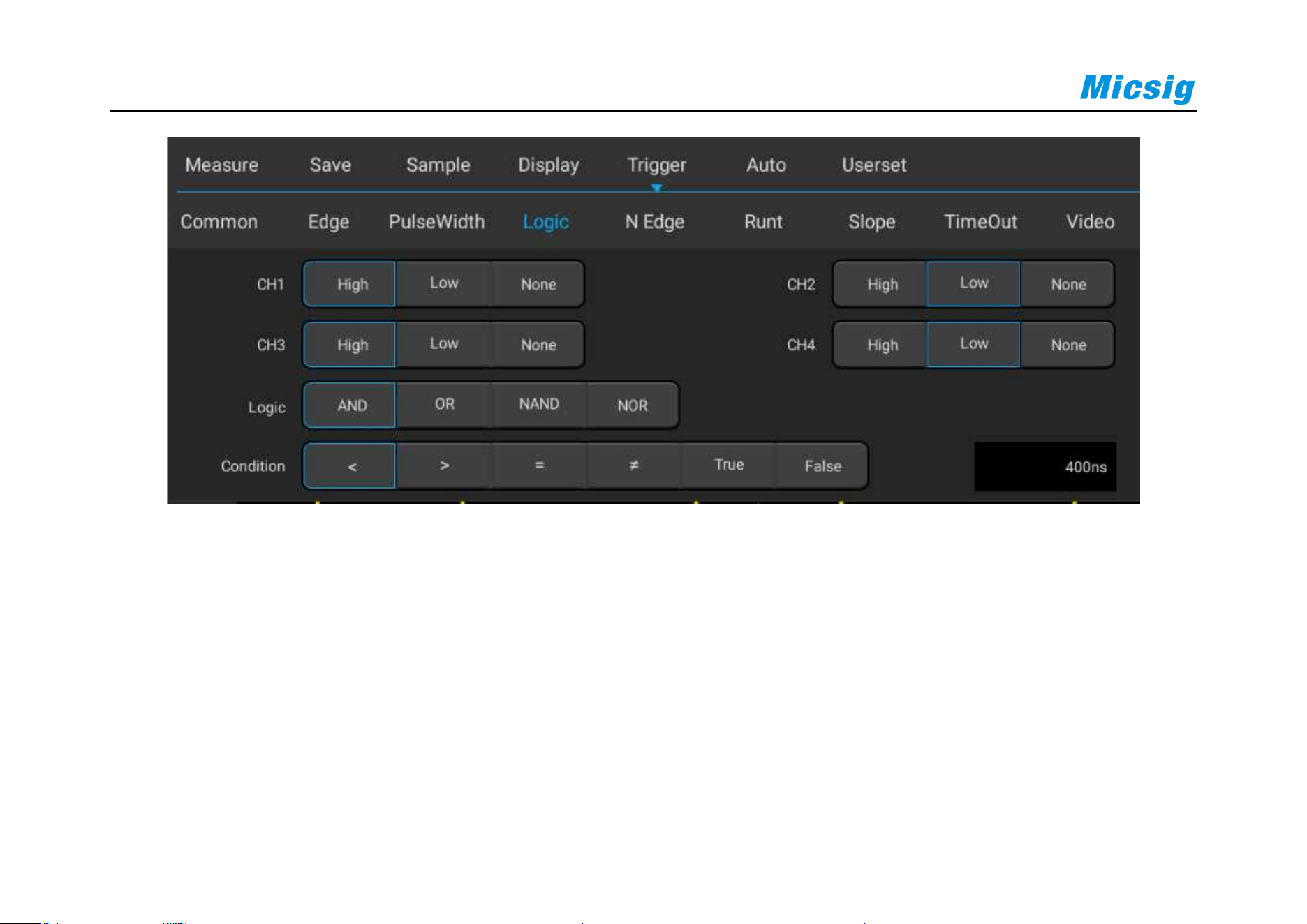
202
Figure 6-21 Logic Trigger Setting Menu
Logic trigger setting description:
Logic level setting
After trigger source, select High, Low and None for the channel. The corresponding trigger level value is
displayed in the upper right corner of the display screen.

Chapter 6 Trigger System
203
High: means a value higher than the current trigger level, and the icon indication is “ ”.
Low: means a value lower than the current trigger level, and the icon indication is “ ”.
None: This channel is invalid.
Switch the trigger level channel: Tap the trigger level slide bar arrow or use trigger setting shortcut
Logic conditions
1) True: Trigger when the logic changes to true value
2) False: Trigger when the logic changes to false value
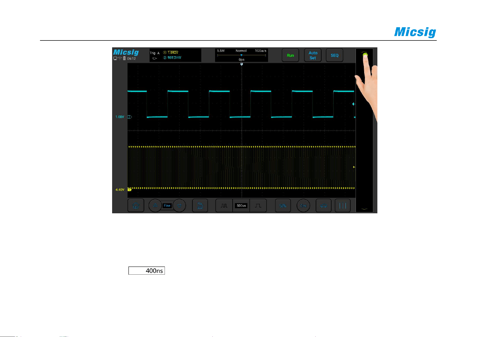
204
Figure 6-22 Trigger Level Adjustment
Trigger pulse width time can be set as 8ns~10s.
Tap the time setting box ( ) to pop up the time adjustment interface and adjust the logic time. Please refer
to the Pulse Width Adjustment section for details.

Chapter 6 Trigger System
205
6.5 Nth Edge Trigger
When the trigger signal is triggered on the Nth edge after the specified idle time, it is Nth edge trigger. Menu
descriptions of the Nth edge trigger are shown in the table below:
Trigger Option
Setting
Description
Trigger Source
CH1
Set CH1 as trigger signal source
CH2
Set CH2 as trigger signal source
CH3
Set CH3 as trigger signal source
CH4
Set CH4 as trigger signal source
Time
8ns~10s
Idle time
Edge
Rising edge
Set signal trigger on the rising edge
Falling edge
Set signal trigger on the falling edge
Nth Edge
1~65535
Set trigger on Nth edge after idle time

206
Set CH1 to trigger on the 5th rising edge after 500us. The steps are as follows:
1) Tap “Trigger” on the main menu to open the trigger menu, select Nth edge trigger in the trigger type, and set
the Nth edge trigger as follows, as shown in Figure 6-23:
Trigger source: CH1;
Time: 10ms;
Edge signal: rising;
Nth edge: 99
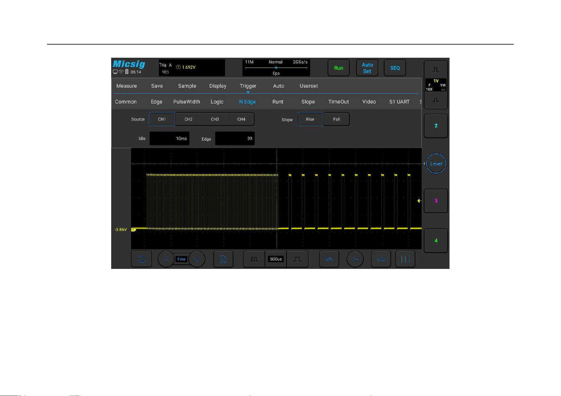
Chapter 6 Trigger System
207
Figure 6-23 Nth Edge Trigger Menu
2) Adjust the trigger level to ensure that the waveform can be triggered stably, for example the trigger level is set
to 1.44V.
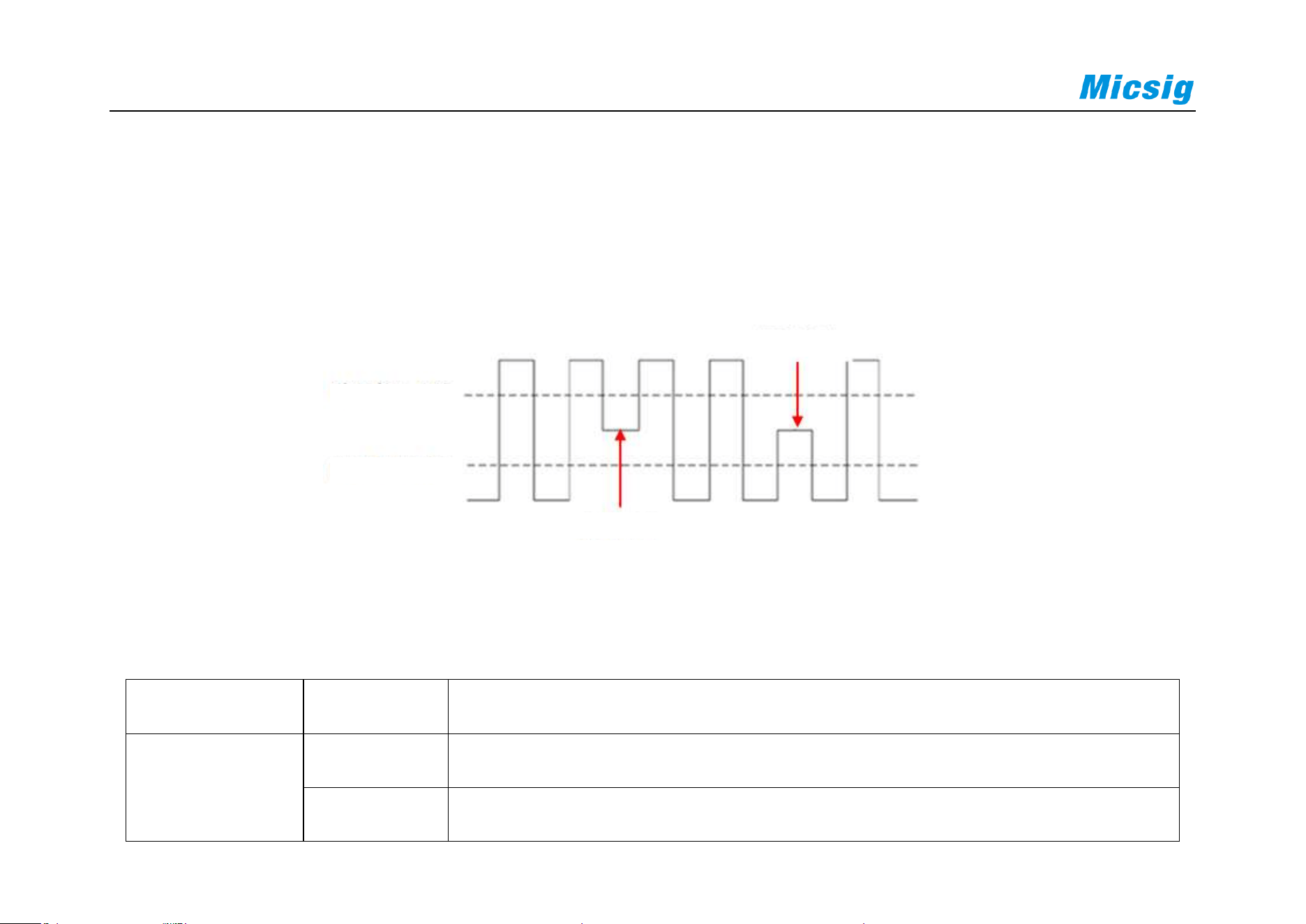
208
6.6 Runt Trigger
By setting the high and low thresholds, trigger on a pulse that cross one threshold but fail to cross a second
threshold. There are two types available: positive short pulse and negative short pulse.
Figure 6-24 Runt Trigger
Runt trigger menu descriptions are shown in the table below:
Trigger Option
Setting
Description
Trigger Source
CH1
Set CH1 as trigger signal source
CH2
Set CH2 as trigger signal source
High Level
Low Level
Positive Short Pulse
Negative Short Pulse

Chapter 6 Trigger System
209
Trigger Option
Setting
Description
CH3
Set CH3 as trigger signal source
CH4
Set CH4 as trigger signal source
Polarity
Positive
Set signal to trigger on positive runt pulse
Negative
Set signal to trigger on negative runt pulse
Any
Set signal to trigger on either positive or negative runt pulse
Trigger
Condition
<T
Trigger when the signal pulse width is smaller than pulse width T
>T
Trigger when the signal pulse width is greater than pulse width T
<>T
Trigger when the signal pulse width is greater than lower limit T1 and
smaller than upper limit T2
None
No trigger restrictions for runt pulse trigger
Trigger Pulse
Width
8ns~10s
Set the trigger pulse width
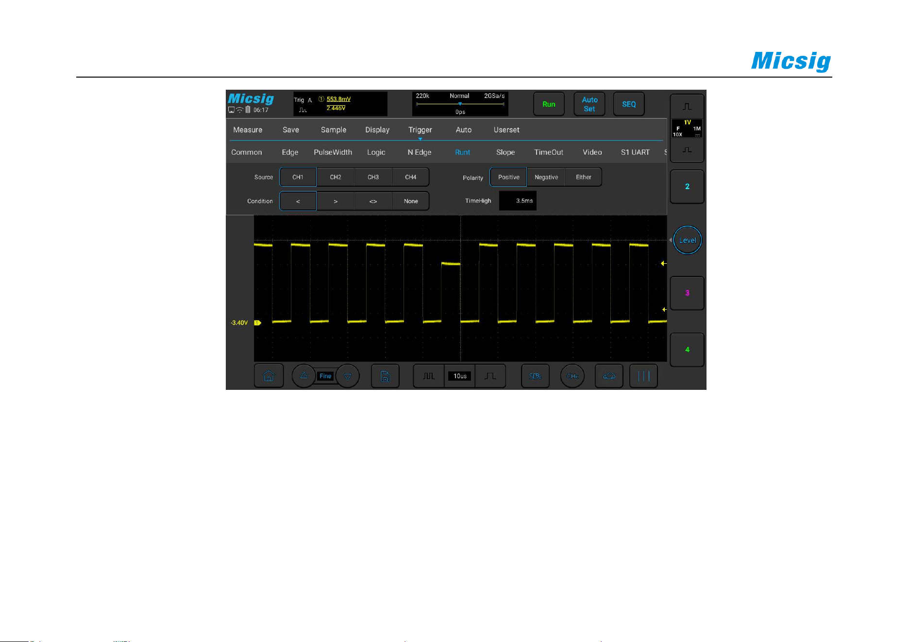
210
Figure 6-25 Runt Trigger Setting Menu
6.7 Slope Trigger
Slope Trigger means trigger when the waveform reaches a set time condition from one level to another.
Positive slope time: Time takes for the waveform to go from low to high.
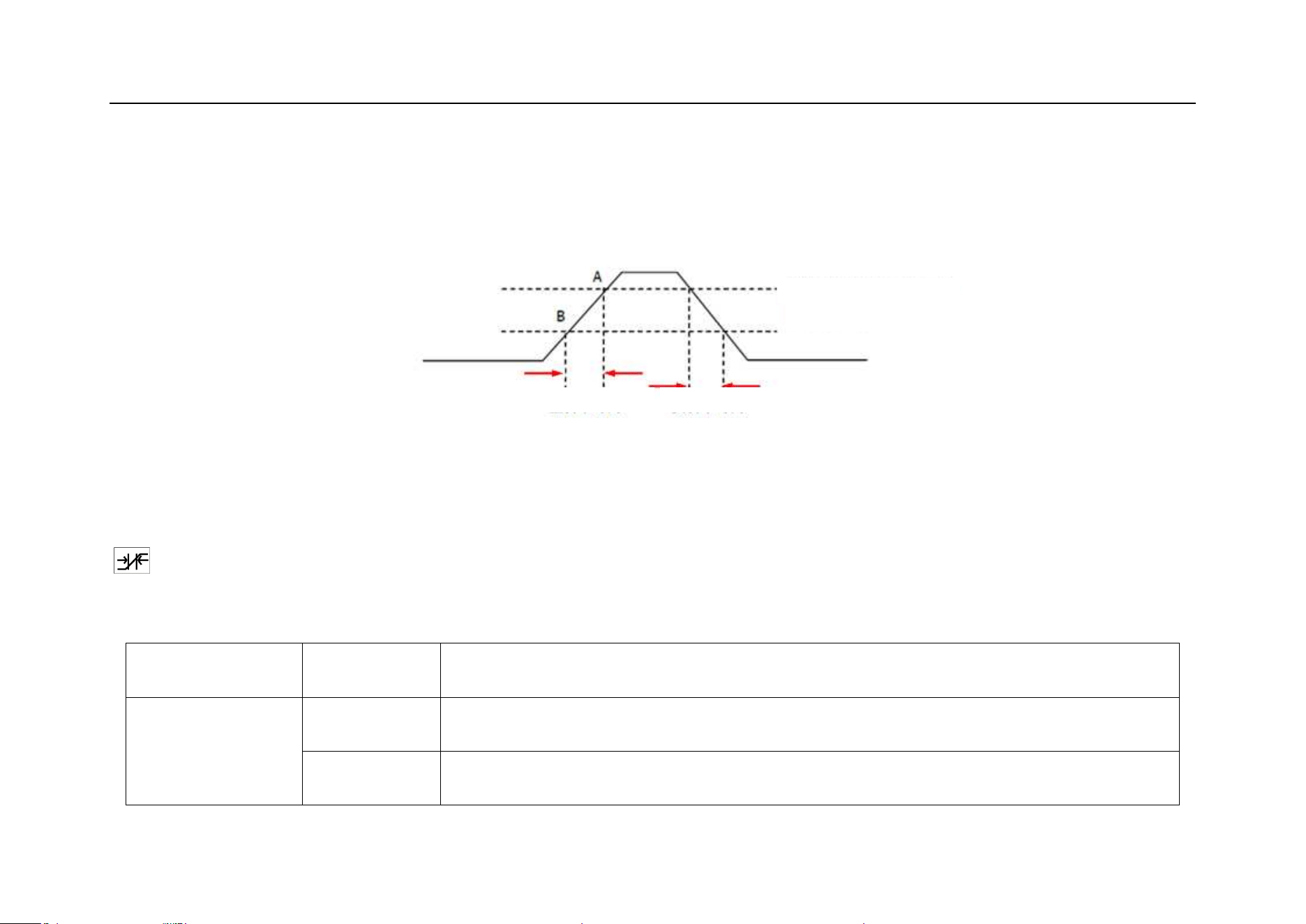
Chapter 6 Trigger System
211
Negative slope time: Time takes for the waveform to go from high to low.
As shown in Figure 6-26
Figure 6-26 Positive/Negative Slope Time
When the trigger signal slope has the hold time (8ns~10s), the trigger type on the top of the screen is only the icon
, and trigger happens when the set condition is reached. Slope trigger is suitable for observing sawtooth or
triangular waves. The slope trigger menu descriptions are shown in the table below:
Trigger Option
Setting
Description
Trigger Source
CH1
Set CH1 as trigger signal source
CH2
Set CH2 as trigger signal source
High Level
Positive Slope Time
Negative Slope Time

212
Trigger Option
Setting
Description
CH3
Set CH3 as trigger signal source
CH4
Set CH4 as trigger signal source
Edge
Rising
Set trigger on positive signal slope
Falling
Set trigger on negative signal slope
Any
Set trigger on detecting a signal slope change
Trigger
Condition
<T
Trigger when the signal slope hold time is smaller than T
>T
Trigger when the signal slope hold time is greater than T
<>T
Trigger when the signal slope hold time is smaller than upper limit T1 and
greater than lower limit T2
Time
8ns~10s
Set the trigger signal slope hold time
Set CH1 slope status as rise and hold time less than 1ms. The steps are as follows:

Chapter 6 Trigger System
213
1) Tap “Trigger” on the main menu to open the trigger menu, select the slope trigger in the trigger type, and set
the slope trigger as follows, as shown in Figure 6-27:
Trigger source: CH1;
Edge: Rise;
Slope hold time: 1us;
2) Adjust trigger level, adjust High or Low trigger level, click arrow at both ends of the chute Switch the trigger
level between High and Low.

214
Figure 6-27 Slope Trigger Setting Menu
The slope hold time can be set as 8ns~10s.
Note: A stable trigger waveform can only be obtained by selecting the channel to which signals are connected as
trigger source.
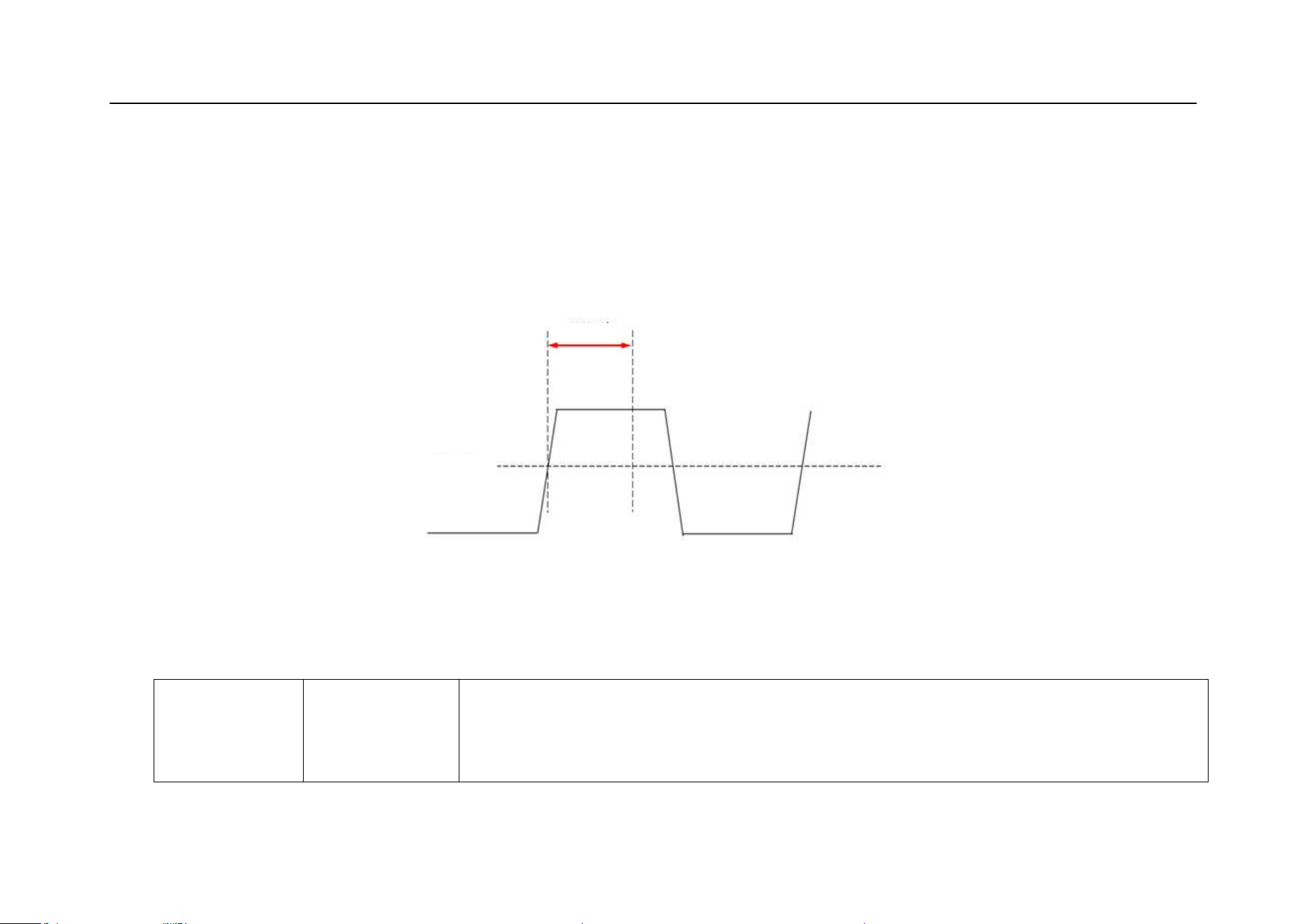
Chapter 6 Trigger System
215
6.8 Timeout Trigger
Timeout trigger happens when the time from the intersection of signal and trigger level and above (or below) the
trigger level reaches the set time, as shown in Figure 6-28:
Figure 6-28 Timeout Trigger Schematics
Timeout trigger menu descriptions are shown in the table below:
Trigger
Option
Setting
Description
Duration
Set Level

216
Trigger
Source
CH1
Set CH1 as trigger signal source
CH2
Set CH2 as trigger signal source
CH3
Set CH3 as trigger signal source
CH4
Set CH4 as trigger signal source
Polarity
Positive
Select to count time when the rising edge of input signal gets through the
trigger level
Negative
Select to count time when the falling edge of input signal gets through the
trigger level
Any
Select to count time when the rising edge or falling edge of input signal gets
through the trigger level
Time
8ns~10s
Timeout time
Set the polarity of CH1 trigger signal to be positive and the timeout time as 15us. The steps are as follows:

Chapter 6 Trigger System
217
1) Tap “Trigger” on the main menu to open the trigger menu, select timeout trigger in the trigger type, and set the
timeout trigger as follows, as shown in Figure 6-29:
Trigger source: CH1;
Edge: positive;
Timeout time: 8ns;
2) Adjust the trigger level to ensure that the waveform can be triggered stably.
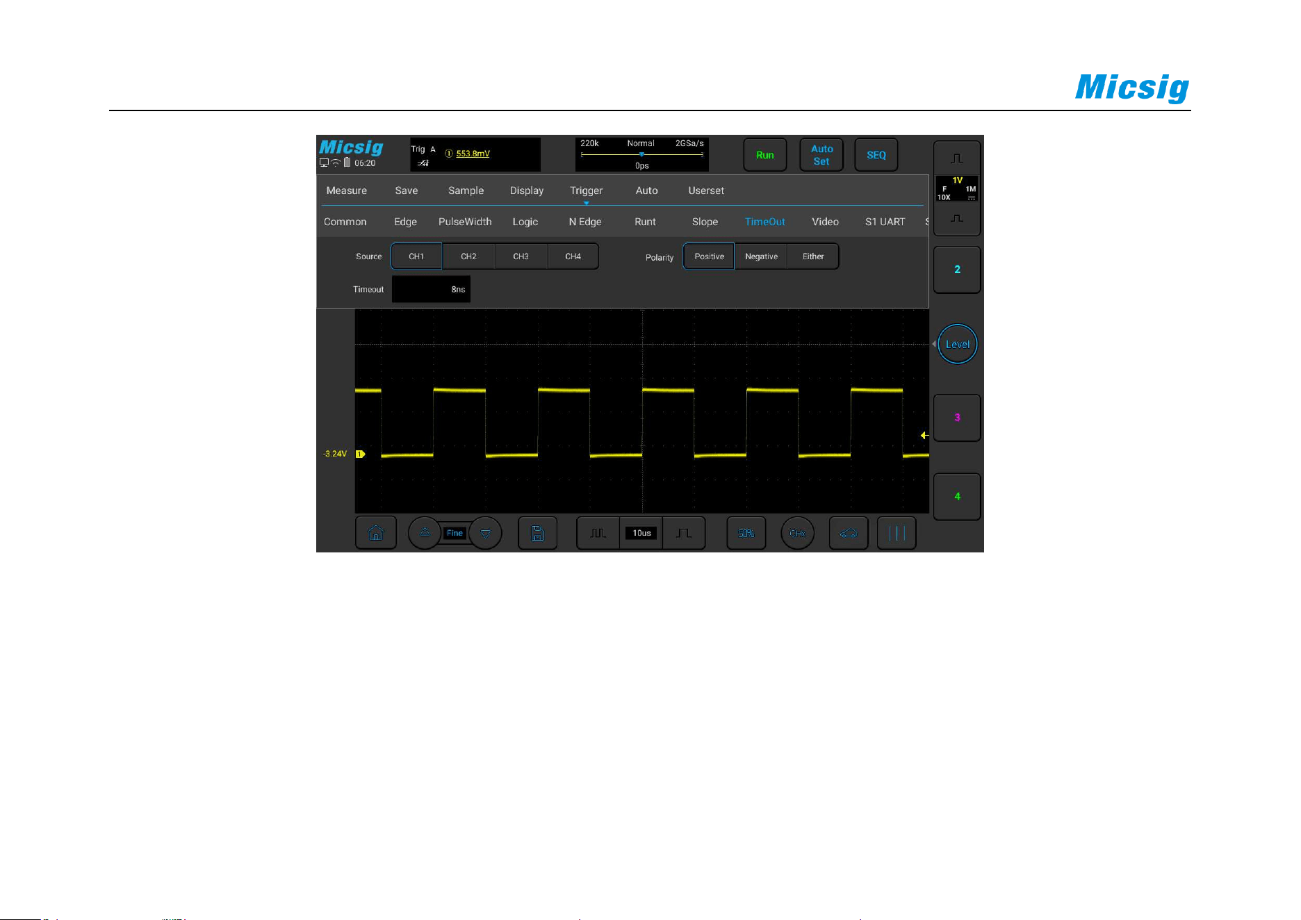
218
Figure 6-29 Time-out Trigger
6.9 Video Trigger
The triggering method for video signals depends on video formats. Generally, there are PAL/625, SECAM,
NTSC/525, 720P, 1080I and 1080P formats. The video trigger can be triggered at different voltage scales, and the

Chapter 6 Trigger System
219
appropriate voltage scale can be adjusted as needed to observe the waveform. The video trigger menu descriptions
are shown in the table below:
Trigger
Option
Setting
Description
Trigger
Source
CH1
Set CH1 as trigger signal source
CH2
Set CH2 as trigger signal source
CH3
Set CH3 as trigger signal source
CH4
Set CH4 as trigger signal source
Polarity
Positive
Set signal positive polarity trigger
Negative
Set signal negative polarity trigger
Video
Standard
625/PAL
Based on PAL signal trigger
SECAM
Based on SECAM signal trigger

220
525/NTSC
Based on NTSC signal trigger
720P
Base on 720P(50Hz, 60Hz) signal trigger
1080I
Base on 1080I(50Hz, 60Hz) signal trigger
1080P
Base on 1080P (24Hz, 25Hz, 30Hz, 50Hz, 60Hz)
signal trigger
Line
Trigger lines
Trigger
Odd fields
Trigger on the rising edge of the first tooth pulse
in odd fields
Even fields
Trigger on the rising edge of the first tooth pulse
in even fields
All fields
Trigger on the rising edge of the first tooth pulse
found
All lines
Trigger on all horizontal sync pulses

Chapter 6 Trigger System
221
Lines
625 line (PAL,SECAM)
Trigger on a specified line in odd or even fields
263 odd line 262 even line
(NTSC)
750 line (720P)
1125 line (1080I,1080P)
Set CH1 as trigger channel, positive polarity, NTSC standard video, all fields trigger, and the steps are as
follows:
Tap “Trigger” on the main menu to open the trigger menu, select the video trigger in the trigger type, and set the
video trigger as follows, as shown in Figure 6-30:
Trigger source: CH1;
Polarity: positive;
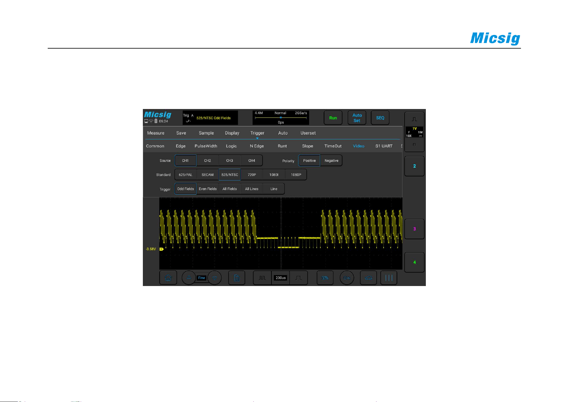
222
Standard: 525/NTSC;
Trigger: Odd fields
Figure 6-30 Video Trigger
Prompts:
In order to better observe the waveform details in the video signal, first set the memory depth to be larger.

Chapter 6 Trigger System
223
During the trigger debugging of the video signal, since the digital oscilloscope has multi-level gray scale display
function, different brightness can reflect the frequency of different parts of the signal. Experienced users can
quickly judge the quality of the signal during the debugging process and find abnormal conditions.
6.10 Serial Bus Trigger
Please refer to
Chapter 12 Serial Bus Trigger and Decode (Optional)

224
Chapter 7 Analysis System
This chapter contains the detailed information of the analysis system of the oscilloscope. You are recommended to
read this chapter carefully to understand the set functions and operation of the analysis system of the ATO series
oscilloscope.
Automatic measurement
Frequency meter measurement
Cursor
Phase Rulers

Chapter 7 Analysis System
225
7.1 Automatic Measurement
Measurement setting
Slide down from top, open the main menu, tap “Measure” to enter the measurement menu. There are 23
measurement items on the measurement menu. Measurement menu, selected measurement item display and
measurement item display are shown in Figure 7-1:
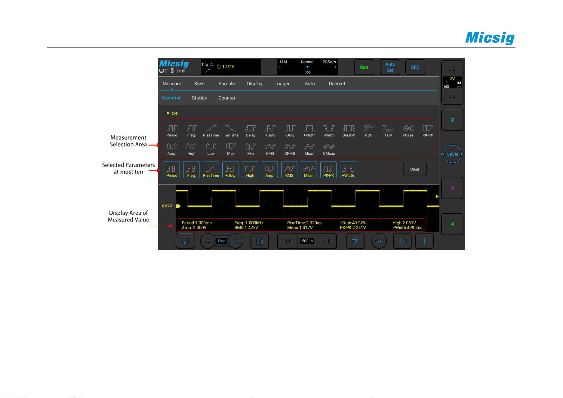
226
Figure 7-1 Automatic Measurement Menu
Automatic measurement
1) Select channel: Select the channel to be measured above the measurement menu.

Chapter 7 Analysis System
227
2) Select measurement: Select the desired measurement item on the measurement menu. The selected
measurement item is displayed in the “Selected Parameters” display area below.
3) Cancel measurement item: In the “Selected Parameters” display area below measurement menu, tap the
measurement item to be cleared; or tap button to clear all measurement items.
Note:
Measurements and math functions will be recalculated when moving/zooming and opening/closing channels.
Oscilloscope has an automatic measurement memory function. Shutdown and restart will not automatically clear
added automatic measurement options.
All measurements
Slide from bottom, open the pull-up menu, see Figure 7-2, click to open all measurement items, display
the current channel measurement value. Switch the current channel to open all the measurement items of other
channels, as shown in Figure 7-3; click again to turn off all measurements.
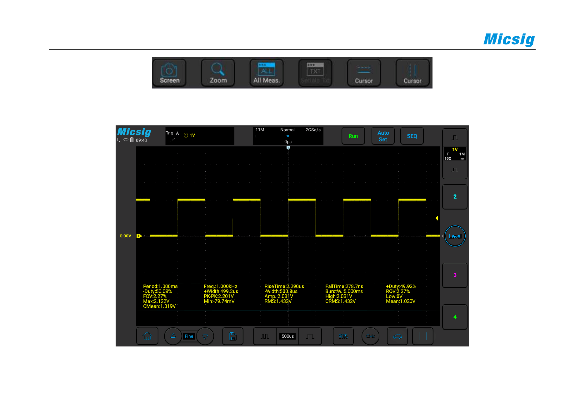
228
Figure 7-2 Pull-up Menu
Figure 7-3 All Measurements
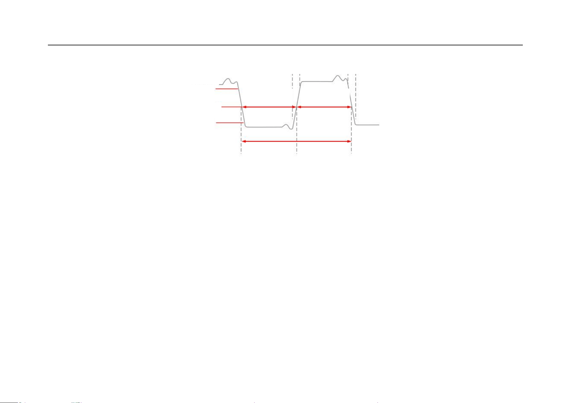
Chapter 7 Analysis System
229
Figure 7-4 Time Parameter
Period
Time of the first complete signal cycle in the waveform
Frequency
Reciprocal to the cycle time
Rise time
Time required for the first rising edge of the waveform to rise from the amplitude of 10% to 90%
Threshold Upper Limit
Threshold Median
Threshold Lower Limit
Period
Rise Time
Fall Time
Positive Pulse
Width
Negative Pulse
Width
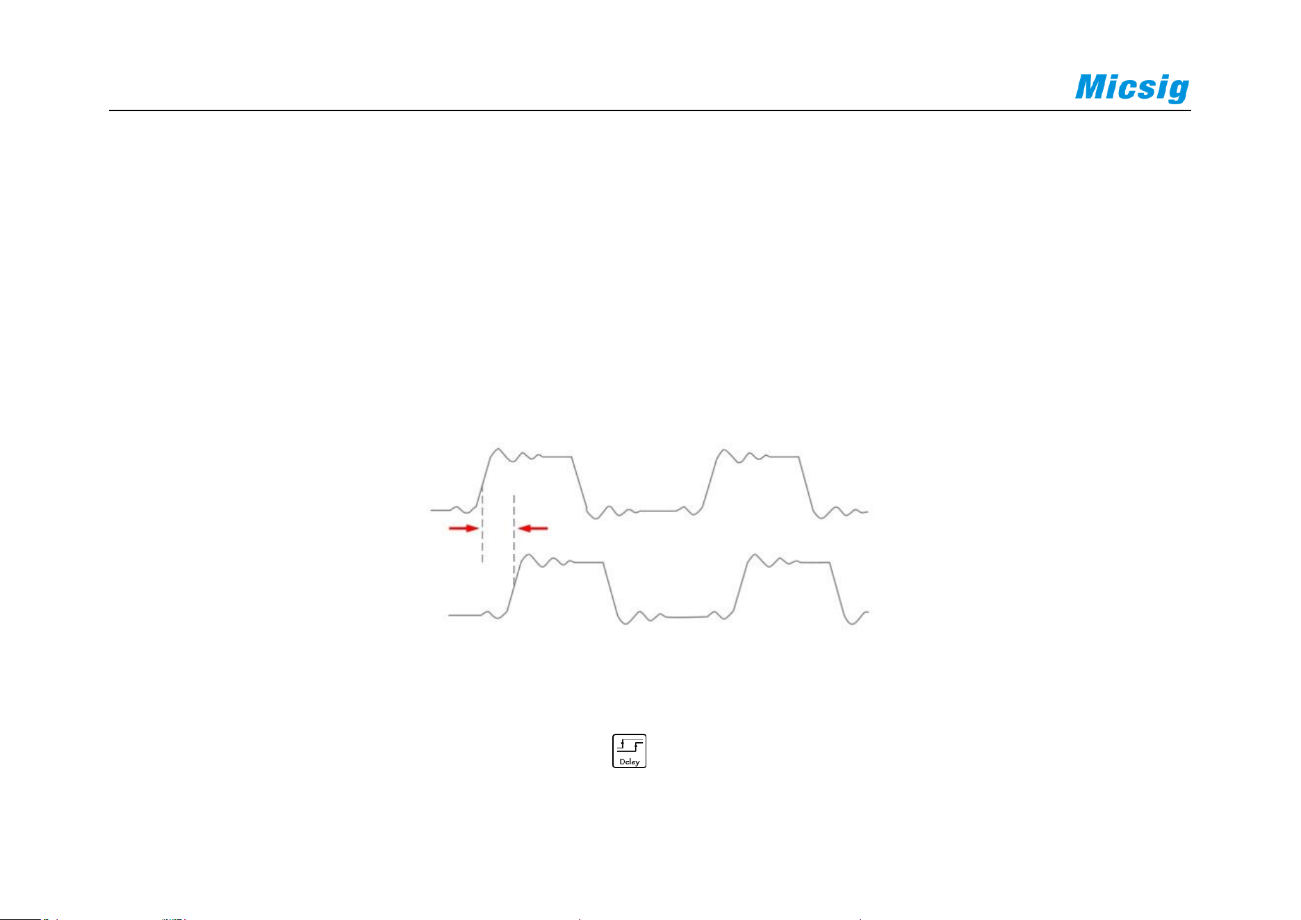
230
Fall time
Time required for the first falling edge of the waveform to rise from the amplitude of 10% to 90%
Delay
Time delay between rising or falling edges of channels may be measured, and there are nine effective measurement
combinations
Figure 7-5 Delay Measurement Schematics
1) Open the automatic measurement menu and tap to pop up the phase selection menu.
Delay

Chapter 7 Analysis System
231
2) The left channel is defaulted as the current channel, and other channels can be selected by the channel area that
has been opened (except the reference channel); there are four edge selections: first rising edge, first falling
edge, last rising edge, last falling edge .
3) The right channel is a contrast delay channel, which can be selected between each channel and math channel.
There are four edge selections: first rising edge, first falling edge, last rising edge, and last falling edge.
4) Tap button to confirm.
Positive duty cycle
Measured value of the first cycle in the waveform
Positive duty cycle = (waveform positive pulse width / period) * 100%
Negative duty cycle
Measured value of the first cycle in the waveform
Negative duty cycle = (waveform negative pulse width / period) * 100%

232
Positive pulse width
Measured value of the first positive pulse in the waveform, taking the time between two 50% amplitude points
Negative pulse width
Measured value of the first negative pulse in the waveform, taking the time between two 50% amplitude points
Burst width
Duration of a burst measured over the entire waveform
Overshoot
Positive overshoot
Positive overshoot =[(max - high) / amplitude]*100%
Negative overshoot
Negative overshoot =[(low - min) / amplitude]*100%
Phase
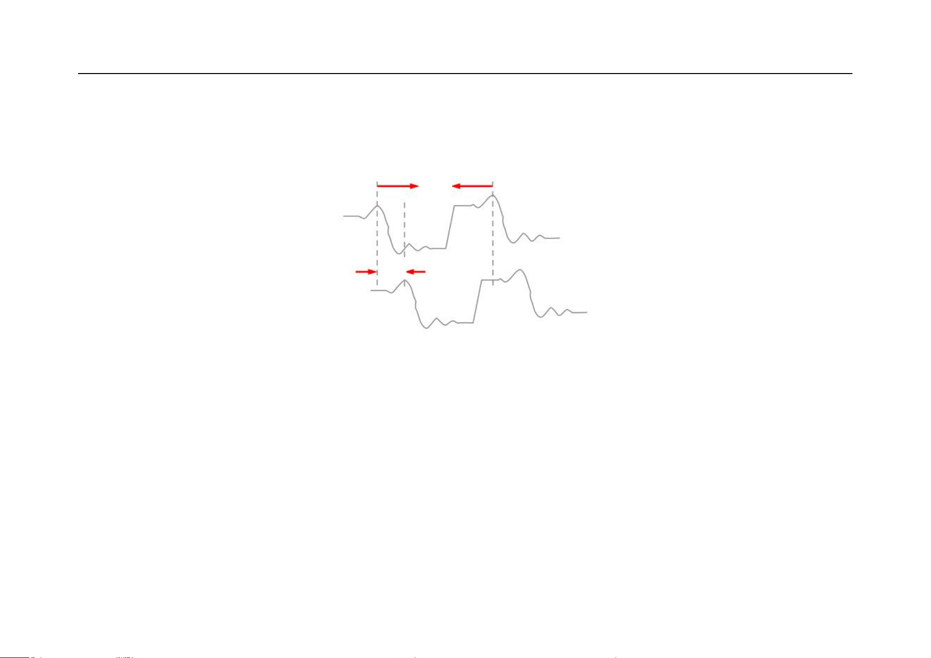
Chapter 7 Analysis System
233
Timing measurement. The amount of time that one waveform leads or lags another waveform, expressed in degrees
where 360°comprises one waveform cycle.
Figure 7-6 Phase Measurement Schematics
Peak-peak
In the entire waveform measurement, peak-peak = max - min
Amplitude
In the entire waveform measurement, amplitude = high (100%) - low (0%)
The figure below shows voltage measurement points.
Delay
Period
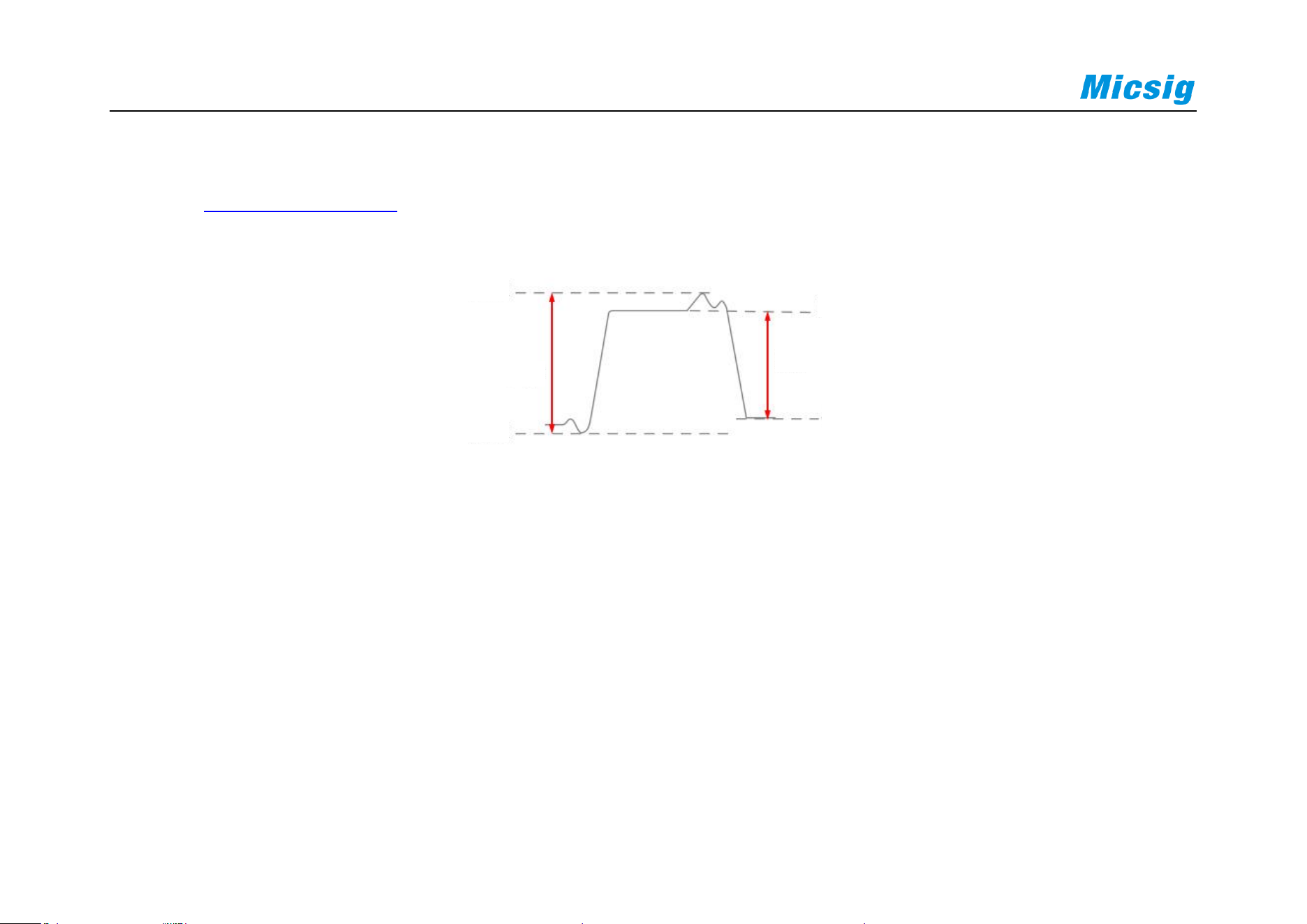
234
The channel probe type setting is used to set the measurement unit for each input channel to Volts or Amperes.
Refer to “
5.4.4 Set Probe Type”.
Figure 7-7 Voltage Measurement
High
Take 100% in the entire waveform, and calculated using either the min/max or histogram method.
Low
Take 0% in the entire waveform, and calculated using either the min/max or histogram method.
Amplitude
Low
Max
Min
Peak-peak

Chapter 7 Analysis System
235
Max
Highest positive peak measured over the entire waveform
Min
Highest negative peak measured over the entire waveform
RMS
True root mean square value over the entire waveform
C RMS
True root mean square value of the first cycle in the waveform
Mean
Arithmetic mean over the entire waveform
C mean
Arithmetic mean over the first cycle in the waveform

236
Note:
If the waveform required for measurement is not fully displayed on the screen, “Forward Clipping” or “Negative
Clipping” is displayed at the position of the measured value.
When the math function is operated, if source channel waveform is fully displayed, and the math waveform appears
to be off the screen, the measured value of math waveform will not be influenced.
If source channel is clipped, the measured value of math waveform is the source channel value during screen wave
clipping.
Statistics
Swipe down from the top to open the main menu, tap "Measure", then select "Statistics" to enter the statistics menu.
The oscilloscope supports statistics and displays the current value of multiple measurement results, including Mean,
Max, Min, Deviation, and Count. The number of counts can be up to 10,000 times. Click the "Reset" button to clear
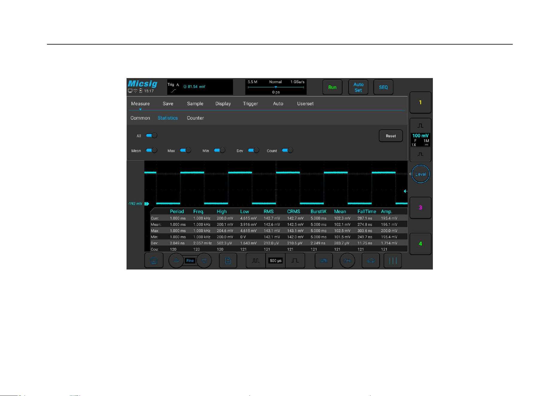
Chapter 7 Analysis System
237
the historical data of all measurement items and perform statistics again, as shown in Figure 7-8:
Figure 7-8 Frequency Meter Measurement Menu Open
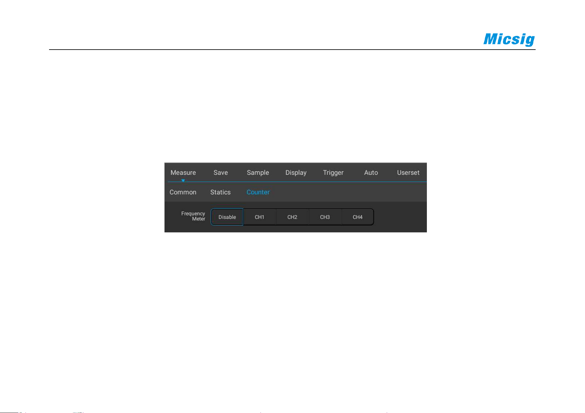
238
7.2 Frequency Meter Measurement
Open the main menu, tap Measure and Counter to enter the hardware frequency meter setting menu, and select the
channel to be measured, as shown in Figure 7-9. The measured value is displayed in the upper left corner of the
screen, as shown in Figure 7-10.
Figure 7-9 Frequency Meter Measurement Menu Open
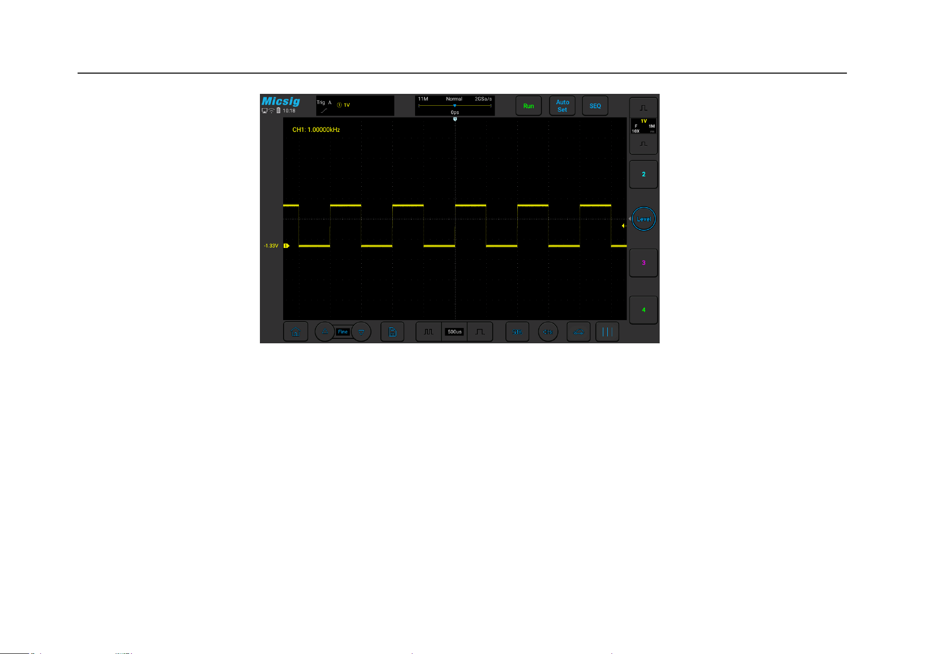
Chapter 7 Analysis System
239
Figure 7-10 Frequency Meter Measurement
7.3 Cursor
Open cursor and place it on the measurement point to read the waveform measurement value. There are two types
of cursors: horizontal cursor and vertical cursor. The horizontal cursor measures the vertical direction magnitude,
and the vertical cursor measures the horizontal direction magnitude, as shown in Figure 7-11.
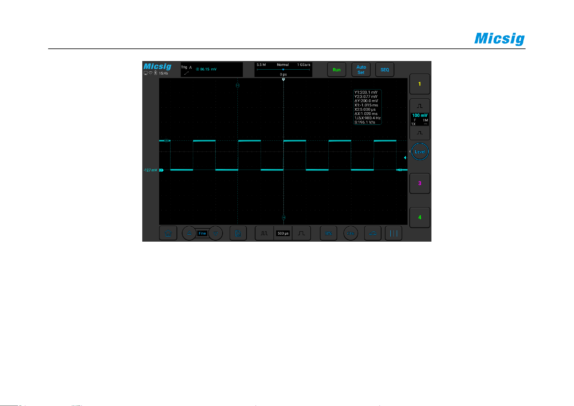
240
Figure 7-11 Cursor Measurement
Note:
reading: indicates the difference between two cursor positions.
Voltage readings after Y1, Y2: indicate the position of activated horizontal cursors relative to the zero
potential.

Chapter 7 Analysis System
241
Time readings after X1, X2: indicate the position of activated vertical cursors relative to the trigger point.
1/
X: frequency
S reading. Indicates the quotient of
(voltage difference) of horizontal cursors and Δ (time difference) of
vertical cursors, that is, the slope of the intersection of the four cursors.
Vertical cursor on/off and activation
Vertical cursor on/off
Vertical cursor on: Open pull-up menu and tap cursor icon to open vertical cursors and the icon is on and
activated.
Vertical cursor off: Open pull-up menu and tap cursor icon to turn off vertical cursors.
Tap the vertical cursor indicator line to switch the cursors.
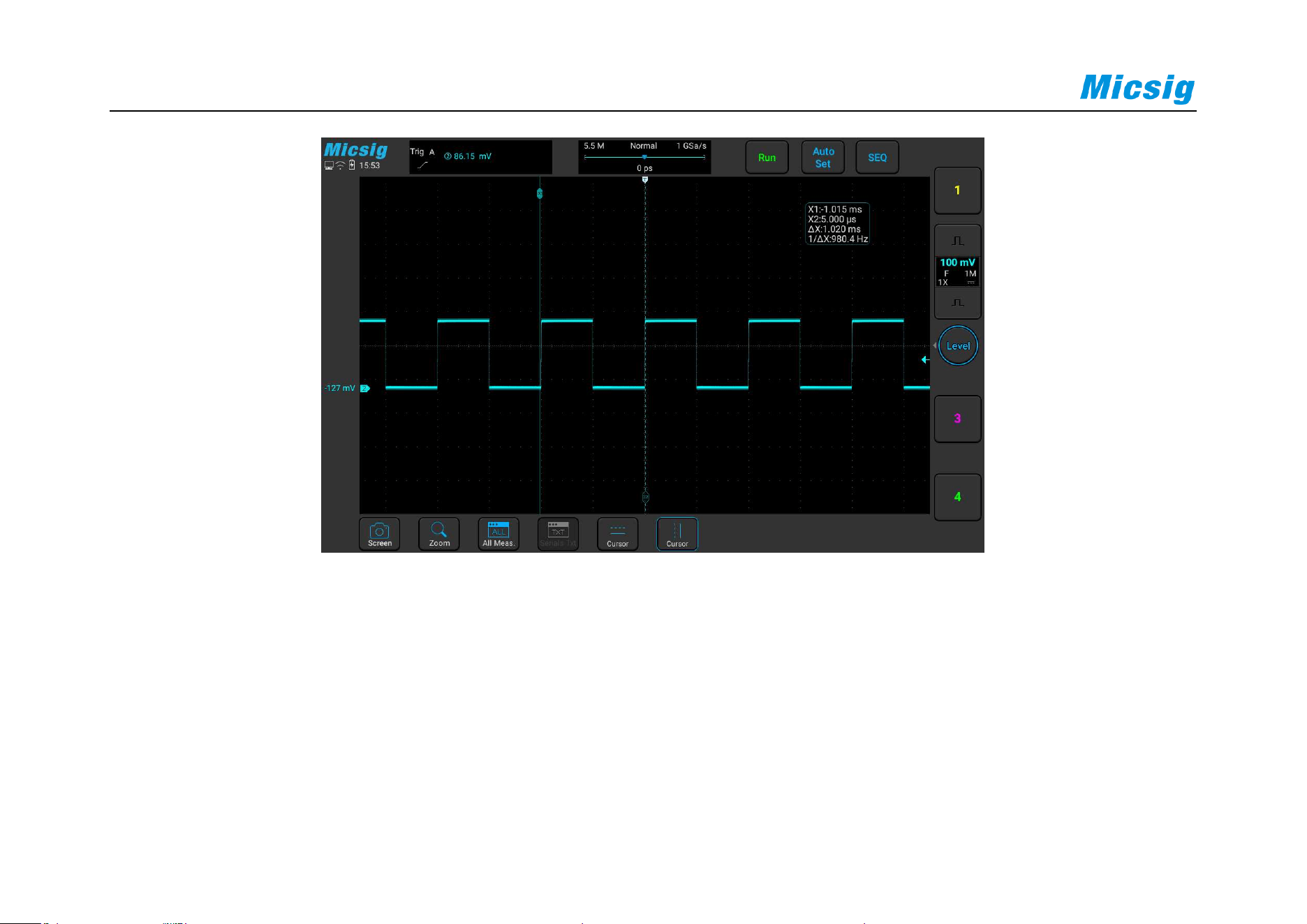
242
Figure 7-12 Open Cursor Selection Box and Close Cursor
Vertical cursor movement descriptions:
1) Use a single finger to press and hold the cursor indicator line on the screen to make coarse adjustment to the
cursor; tap the fine adjustment button in the lower left corner of the screen to fine-adjust the cursor that has
just been adjusted.

Chapter 7 Analysis System
243
2) Cursor linkage: When the cursor is opened, two finger slide and enter the cursor linkage state.
Note: During the sliding process, the current operation is changed unless the initial two fingers leave the
screen. If one finger leaves the screen and the other finger does not leave, the current linkage adjustment is
continued.
Horizontal cursor on/off and activation
Horizontal cursor on/off, switching, activation and movement operations, similar to those of vertical cursors, will
not be described in detail here, and please refer to vertical cursors for details.
Cursor test example
When vertical cursors are activated, the two cursors move together to check for pulse width changes in the pulse
sequence.
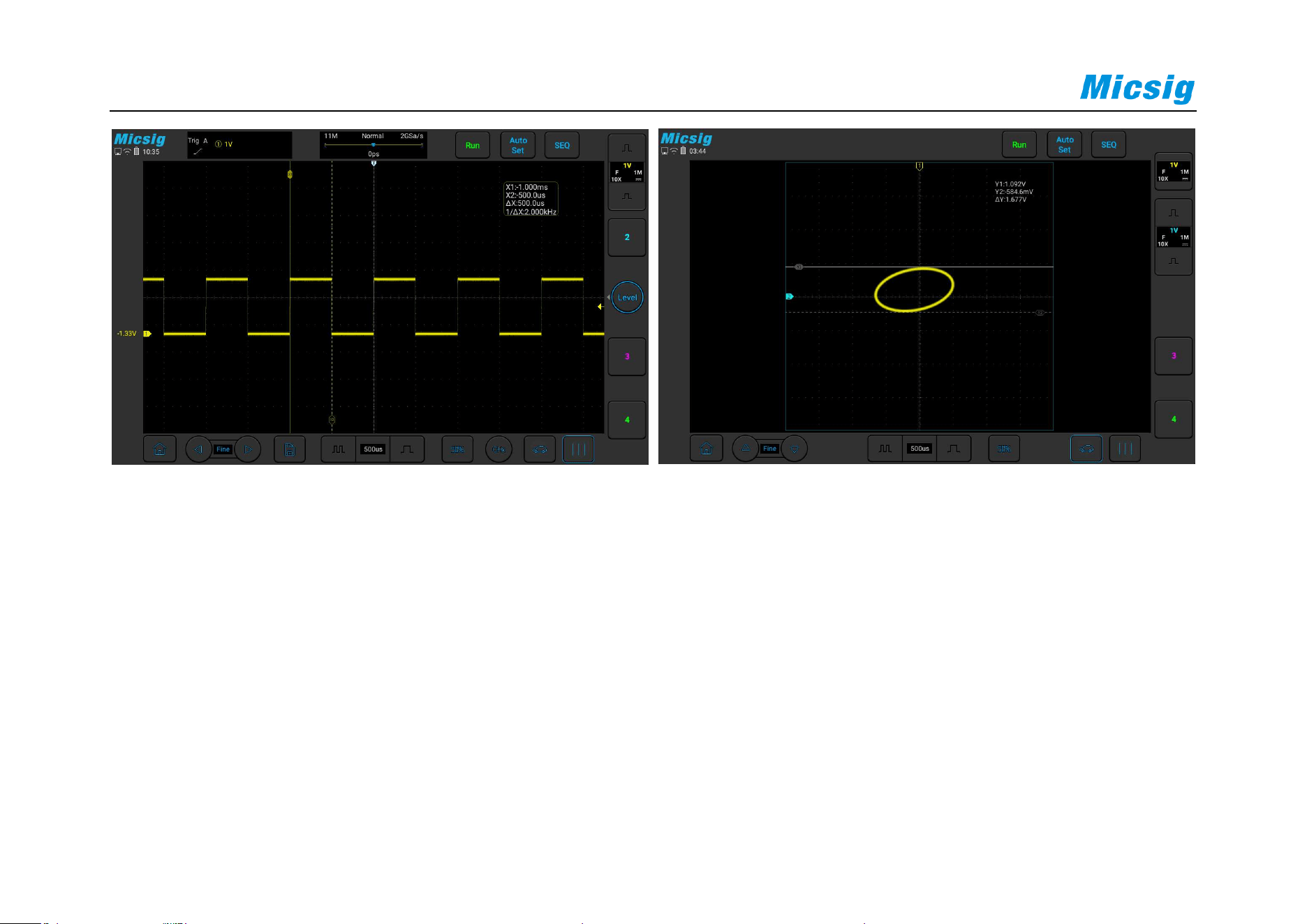
244
Figure 7-13 Cursor Measurement Pulse Width Figure 7-14 In XY Mode, Cursor Measurement
In the XY horizontal mode, X cursor displays CH1 value (V or A), and Y cursor displays CH2 value (V or A).
7.4 Phase Rulers
The phase rulers help to measure the timing of a cyclic waveform on a scope view. Phase rulers measure relative
to the start and end of a time interval that you specify. Phase ruler settings box include Number of cylinder &
Angle. To use the phase rulers, drag the two phase ruler handles onto the waveform from their inactive position.
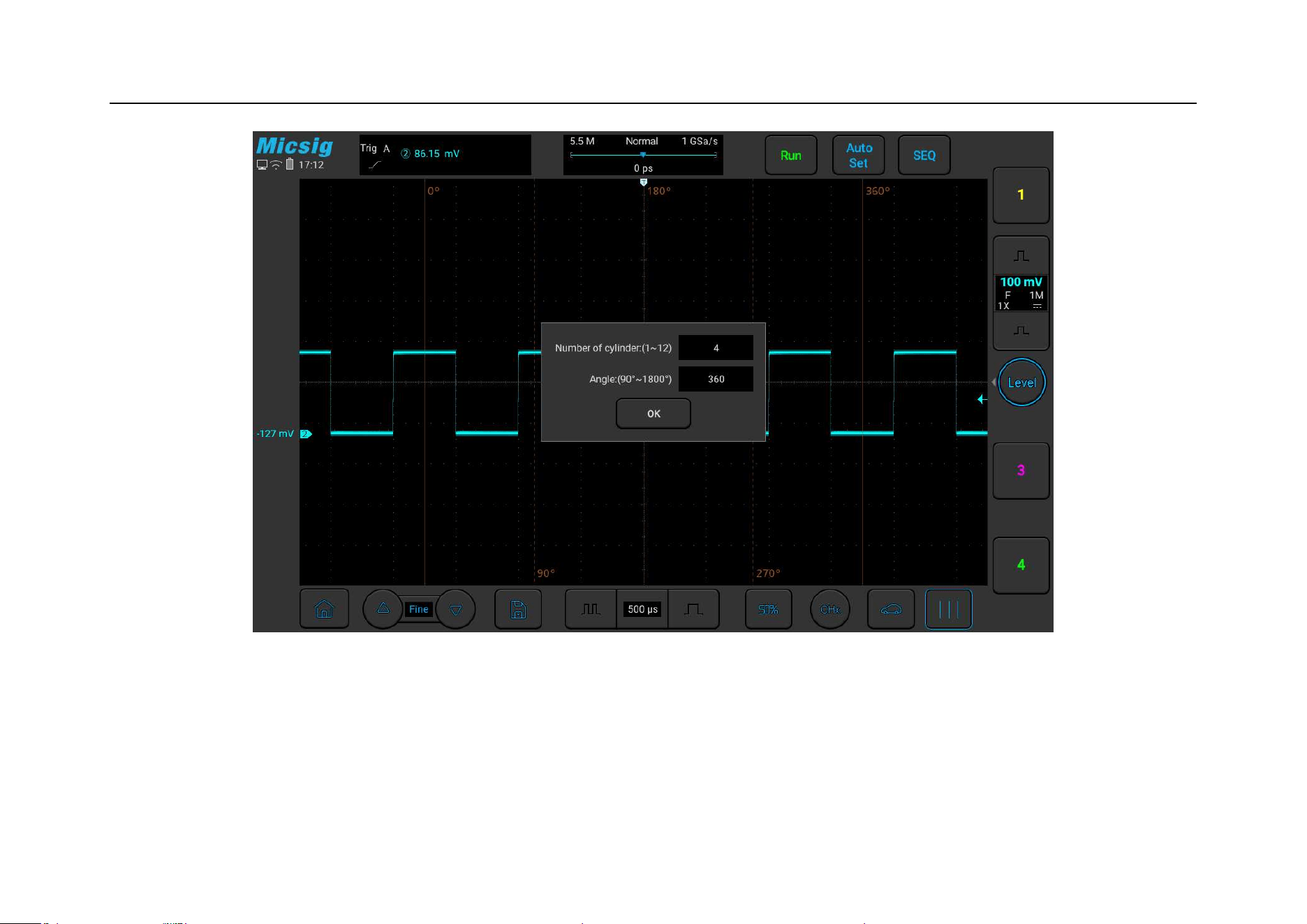
Chapter 7 Analysis System
245
Figure 7-15 Phase Cursors

246
Chapter 8 Screen Capture, Memory Depth and Waveform Storage
This chapter contains the detailed information of the screen capture function and memory depth of the oscilloscope.
You are recommended to read this chapter carefully to understand the storage system of the ATO series
oscilloscope.
Screen capture function
Video recording
Memory depth
Waveform storage

Chapter 8 Screen Capture, Memory Depth and Waveform Storage
247
8.1 Screen Capture Function
The screen capture function can locally store the display information on the current display screen in picture format.
Screen capture method: Slide upward from bottom to open pull-up menu. Tap the icon to have a screen
capture in the oscilloscope application. Or pull down the menu in non-oscilloscope application interface twice and
click the screen capture option to capture the screen content of the non-oscilloscope application.
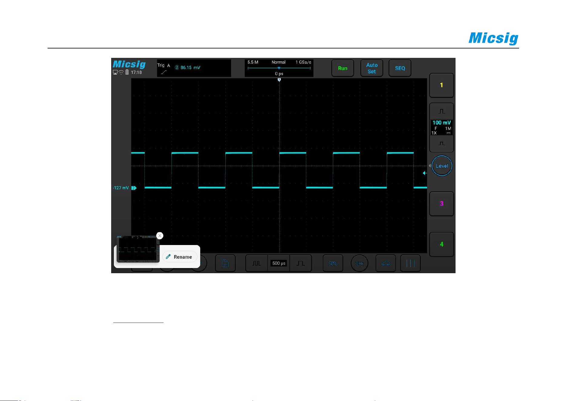
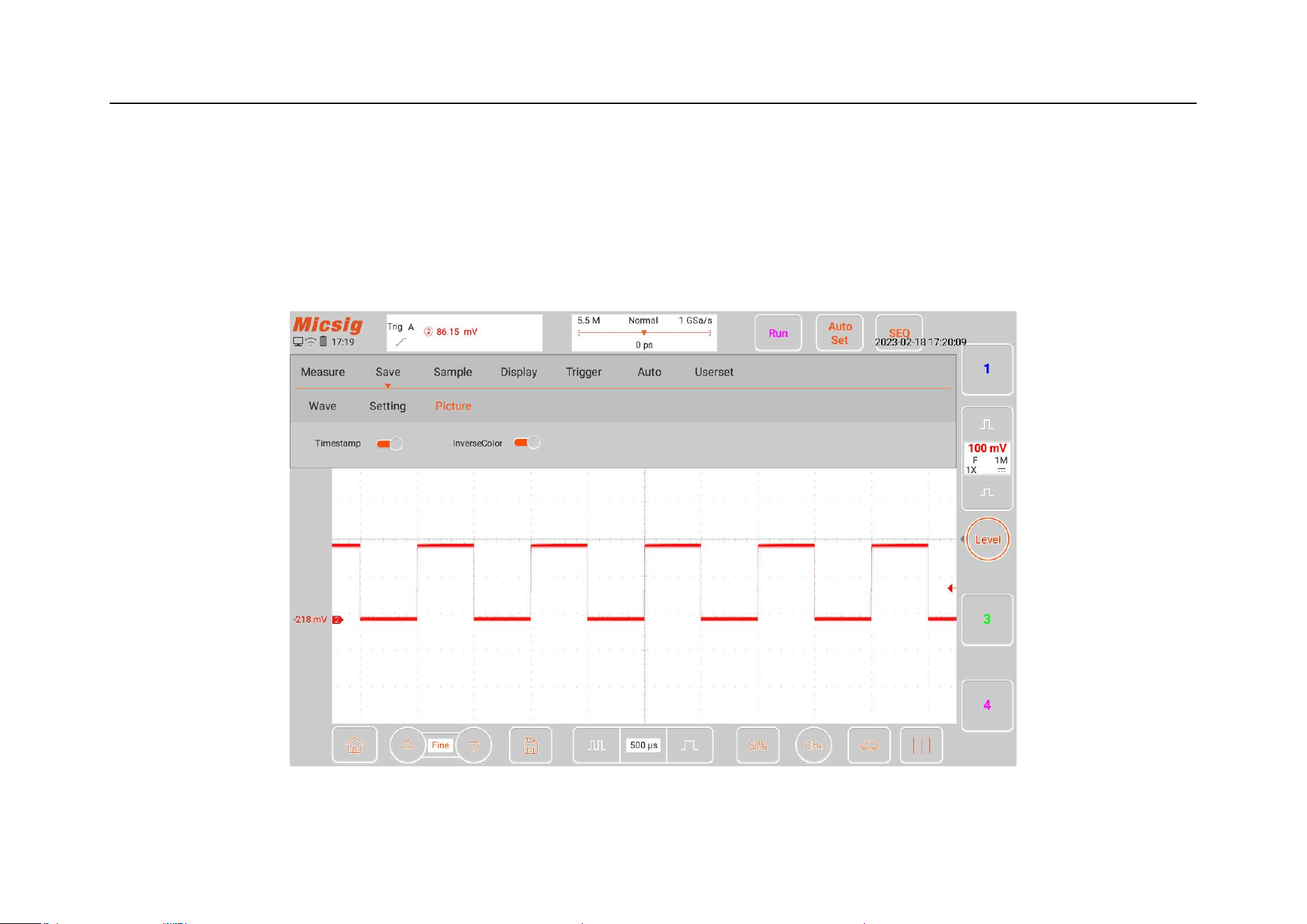
Chapter 8 Screen Capture, Memory Depth and Waveform Storage
249
Timestamp and InverseColor
Invert and time-stamp screenshots is possible in oscilloscope.
Open the main menu, tap Save and enter Picture menu, turn off/on Timestamp and InverseColor button as desired.
Figure 8-2 Timestamp & inverse color

250
8.2 Video Recording
The video recording function is similar to the screen capture function, and the display information of the current
display screen can be stored locally in video format.
Video recording method is sliding down from top in non-oscilloscope application, open pull-down menu, tap the
screen to start recording, and count down to three seconds to complete the video recording, as shown in Figure 8-3.
You can cancel recording by pressing the triangular, circular or square button at the bottom of the screen before the
countdown ends.
During video recording, you can end recording by tapping the video recording time at the top left of the screen. Or
you can leave the oscilloscope application interface to open the pull-down menu, and click “Stop Recording” to end
the video recording.
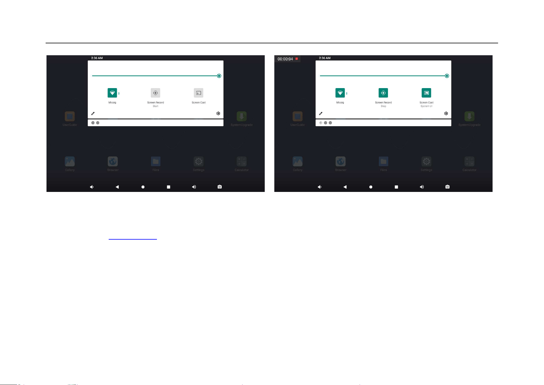
Chapter 8 Screen Capture, Memory Depth and Waveform Storage
251
Figure 8-3 Video Recording Method Figure 8-4 Video Recording
Please refer to “
13.7 Gallery” for details of viewing videos.
8.3 Waveform Storage
The oscilloscope can save the analog channel or math channel waveform locally or in USB device. The file type can
be WAV, CSV or BIN.
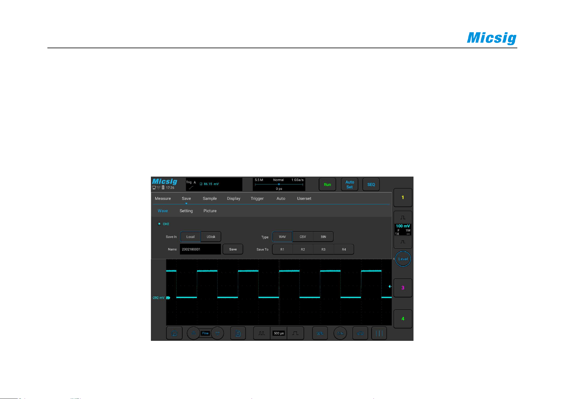
252
The oscilloscope provides four reference channels, which can be called to load WAV format files into the reference
channel and open the reference channel to display the reference waveform.
Save reference file
Slide down from top, open main menu and tap "Save" to open the menu. Save the reference waveform interface of
the specified channel as follows:
Figure 8-5 Save CH2 Reference Waveform Interface

Chapter 8 Screen Capture, Memory Depth and Waveform Storage
253
Location: Stored locally and in USB device.
File types: WAV, CSV, and BIN.
File name: The initial file name is displayed as year + month + day + storage serial number. Press the file name box
to pop up the virtual keyboard, tap “Backspace” to delete the file name, and use the virtual keyboard to rename the
file.
Save: Tap to save the reference file and pop up the save success prompt. The most recently saved file will be
displayed at the top of the called menu.
Save to: Tap the R* (R1, R2, R3, R4) button to save the current channel waveform directly to the corresponding
reference channel, and the save success prompt will pop up.
Back: Tap to return to the previous level.
Method 1: Click the “save” button
In the Save Reference Waveform menu, select the channel waveform to be saved, select the file save location, file
type and file name, and click the “save” button to save the reference waveform file.

254
Save the reference waveform by steps as follows:
1) The current channel is set to the channel to be saved, which can be analog channel, math channel or reference.
2) In the main menu, tap "Save" to enter the save menu.
3) In the Save menu, tap "Save" to open the Save Reference Waveform menu and make the following settings:
Storage location: locally.
Selecting the file type: WAV.
Entering the file name: CH1.
4) Tap “Save” to save the reference file. The save success prompt box is popped up.
If the reference waveform file is to be saved in USB device, the oscilloscope must be connected to an external
USB device. After connection, the reference waveform save location is preferentially set to the USB device.
There is no limit to the number of saved reference waveform files.
Method 2: Click R* button

Chapter 8 Screen Capture, Memory Depth and Waveform Storage
255
In the Save Reference Waveform menu, tap R* (R1, R2, R3, R4) button to save the current channel waveform
directly to the corresponding reference channel, and the save success prompt will pop up. The file name is displayed
as Ref* in the reference channel (* is the corresponding reference channel name). Reference waveform files saved
by this method will be overwritten after loading other reference waveforms and cannot be restored.
Method 3: Click “Quick Save” button
Tap at bottom of the screen to save all channel waveforms as reference waveforms and capture the current
screen. The file names are the default initial file names.
Management of reference files
In the file manager, open waveforms in the classification file to manage reference files by operations such as copy,
cut, delete, rename, compress, etc., as shown in Figure 8-4. Select reference files and click trash button to delete
them; click More at bottom of the screen, tap Rename to open soft keyboard and change the reference file name.
Tap Compress to pop up the soft keyboard and enter the compressed file name to compress the file; when inserting
the USB device, files on the oscilloscope can be moved to the USB device.
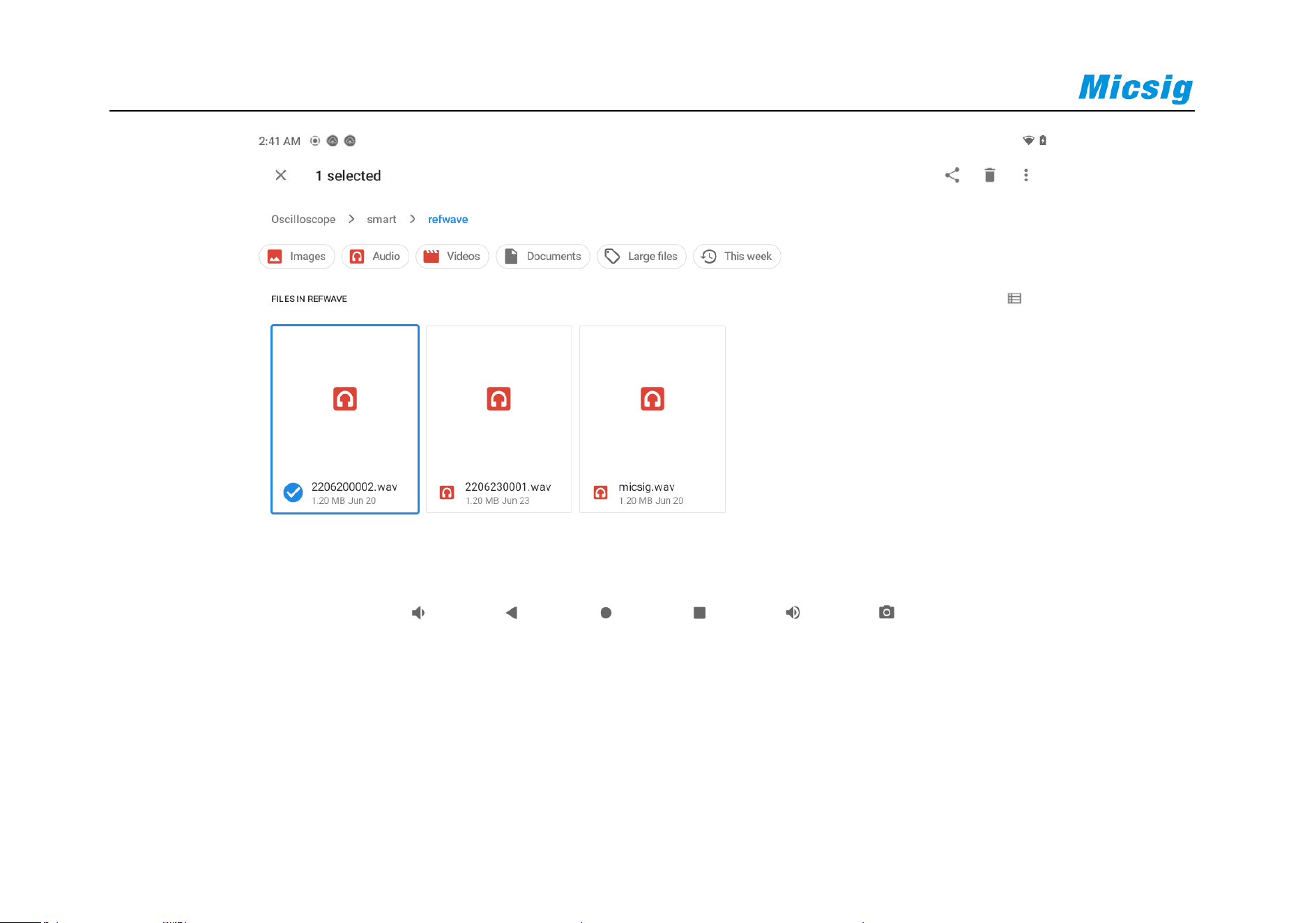
256
Figure 8-6 Delete Reference Files
CSV files
CSV file structure

Chapter 8 Screen Capture, Memory Depth and Waveform Storage
257
CSV format contains the basic information of the saved data: save time, file name, data length, sampling interval,
trigger time, source, vertical scale, vertical offset, vertical accuracy, horizontal time base, horizontal accuracy, probe
multiples.
The data and length of CSV files can be saved up to 70K/35K depending on the single/dual channel while being
saved. If the oscilloscope record length or the displayed data length is less than 70K/35K, the data length of CSV
files changes either. For example, when the record length is set to 14/7/3.5K, there will be 7000 sample points in the
dual channel CSV file.
Max and Min in CSV files
If running Min or Max measurements, Min and Max values displayed on the measurement results screen may not
appear in CSV files.
Explanation: If the oscilloscope sampling rate is 1GSa/s, sampling will be once every 1ns. If the horizontal scaling
is set to 10us/div, the data of 140us will be displayed (because there are 14 divisions on screen). To find the total
number of samples, the oscilloscope will perform: 140us×1GSa/s=140K sampling, which require the oscilloscope

258
to display 140K times of sampling using 600-pixel columns. The oscilloscope extracts 140K samples into 600-pixel
columns, and this extraction will track Min and Max values of all points represented by any given column. These
Min and Max values will be displayed in this screen column.
The similar process is applied to reduce sampled data and produce records that can be used to perform various
analyses, such as measurements and CSV data. This analysis record (or measurement record) is much larger than
600 and may actually contain up to 60,000 points. However, once the number of points sampled exceeds 60,000,
some extraction method is required. The extraction factor used to generate the CSV record is configured to provide
the best estimate of all samples represented by each point in the record. Therefore, Min and Max values do not
appear in CSV files.
8.4 Oscilloscope setting save
The oscilloscope supports saving up to 10 current settings and restoring them with one key.
Open the main menu, tap Save and enter Setting menu, as shown in Figure 8-7.
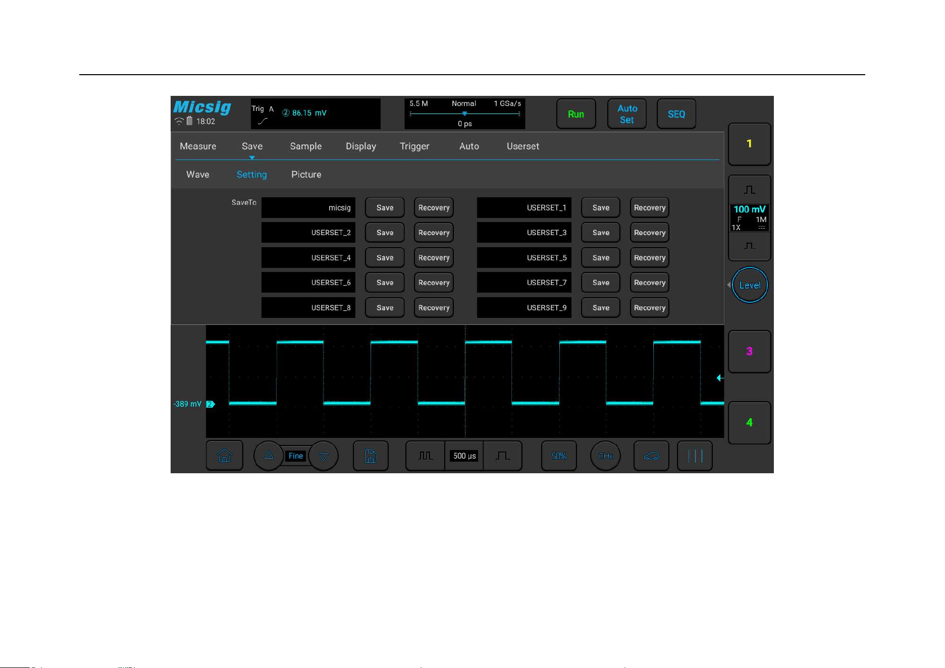
Chapter 8 Screen Capture, Memory Depth and Waveform Storage
259
Figure 8-7 oscilloscope setting save
Tap the black box area to rename save settings, tap the Save button to store, the Recovery button to restore the
settings.

260
Chapter 9 MATH and Reference
This chapter contains the detailed information of the MATH operation and reference channel of the oscilloscope.
You are recommended to read this chapter carefully to understand the setting functions and operations of the MATH
and reference channels of the ATO series oscilloscope.
Dual waveform calculation
FFT measurement
Reference waveform call
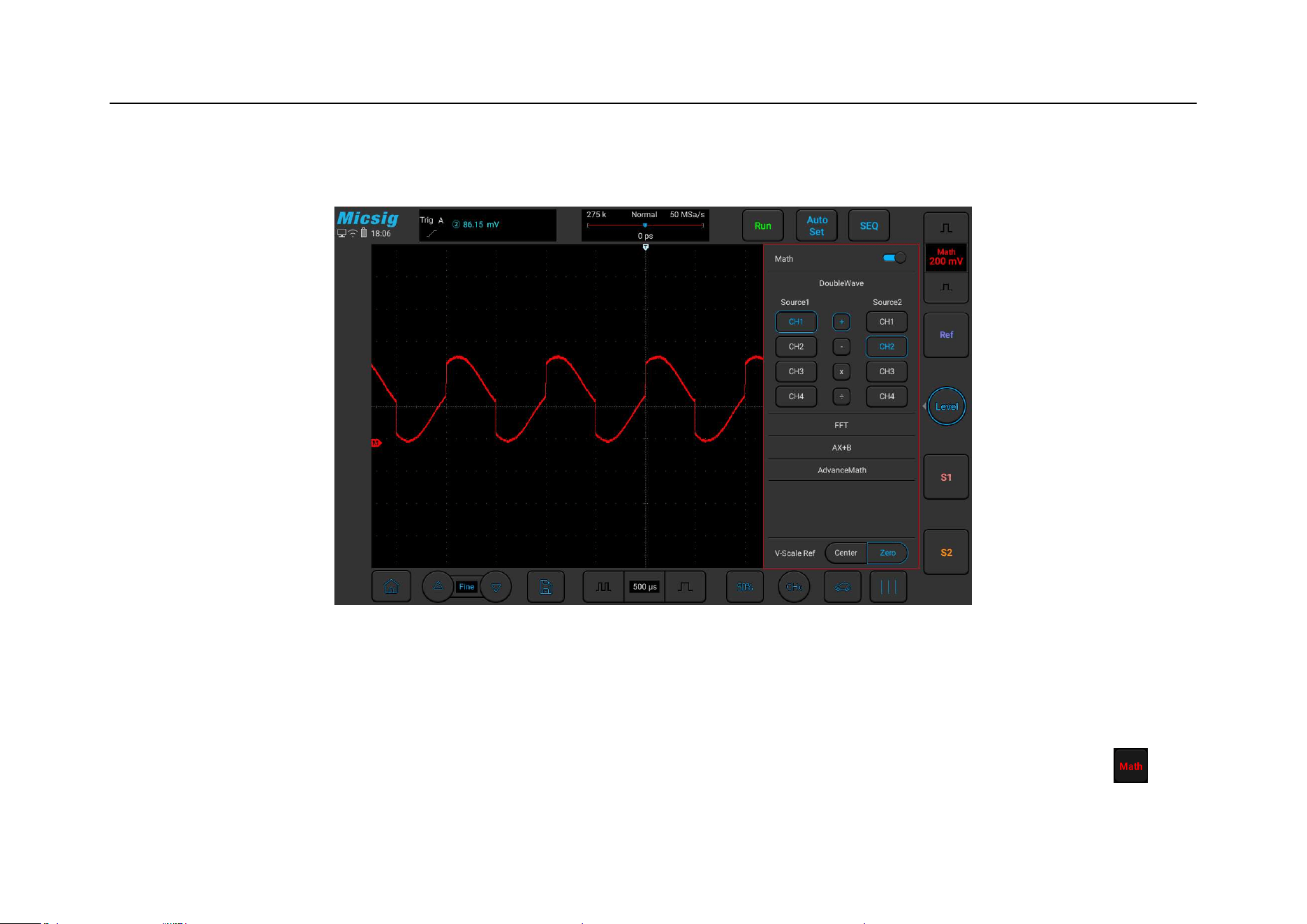
Chapter 9 MATH and Reference
261
9.1 Dual Waveform Calculation
Figure 9-1 MATH Channel Waveform
Display math waveform
Swipe up or down at the channel selection area to enter the second channel selection area. Tap the soft key to
open the math channel. After the math waveform is opened, the current channel selector is automatically opened.

262
Left swipe math channel icon to open the math channel menu. While opening math for the first time, the math
operation is defaulted as the dual channel calculation.
Math operation prompt
If the analog channel or math function is clipped (not fully displayed on the screen), the resulting math function will
also be clipped.
Once the math waveform is displayed, tap the channel icon to close the source channel for a better view of the math
waveform.
The vertical sensitivity and offset of each channel participating in the math function can be adjusted to facilitate
viewing and measuring of the math waveform.
The math function waveform can be measured using “Cursor” and “Measure”.
Adjust the math waveform
1) Press the math channel vertical sensitivity icon, directly tap the math waveform or math channel indication
icon , and set the math channel as the current channel.

Chapter 9 MATH and Reference
263
2) For details of movement, vertical sensitivity adjustment, time base adjustment and vertical expansion reference
of the math channel, please refer to “
Chapter 4 Horizontal System” and “Chapter 5 Vertical System”.
3) The vertical sensitivity, unit and time base corresponding to the math waveform are displayed in the channel
area of the math channel. For details, see “
2.7 Understand the Oscilloscope Display Interface”.
Math waveform units
Use “Probe Type” on the channel menu to adjust the channel unit (refer to “
6.4.4 Set Probe Type”) and set the unit
of each input channel to Volt or Ampere. The units of math function waveform include:
Math Function
Unit
+/-
V, A, ?
×
VV, AA, W
÷
V/V, V/A, A/A, A/V
Table 9-1 List of Mathematical Units

264
Note: If the units of two operation source channels are different and the unit combination cannot be identified, the
unit of math function will be displayed as? (undefined).
Math operators
Math operators perform arithmetic operations on the analog input channels.
Addition or subtraction
If addition or subtraction is selected, the values of function sources 1 and 2 will be added or subtracted point by
point and the results will be displayed.
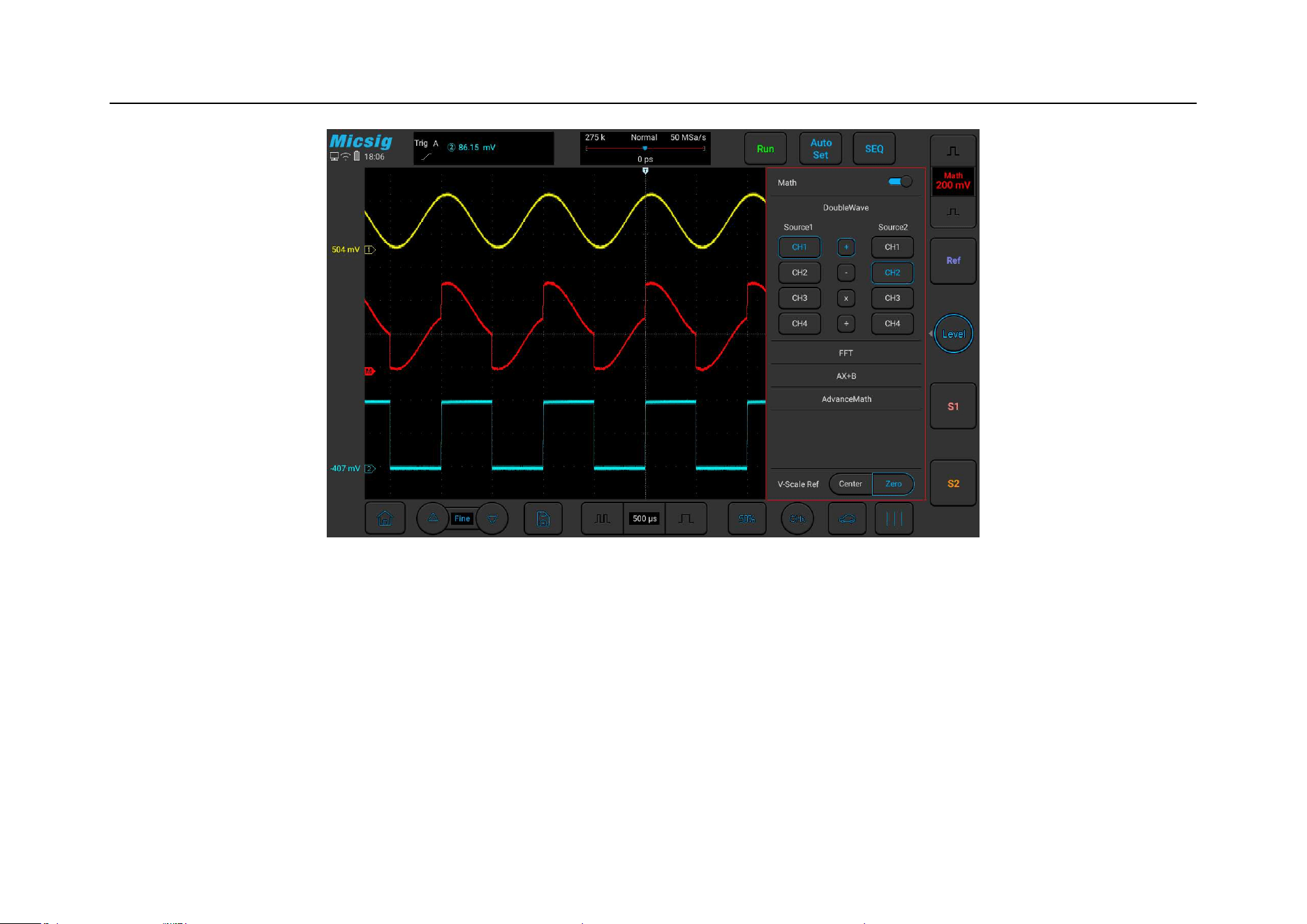
Chapter 9 MATH and Reference
265
Figure 9-2 Mathematical Operation of CH1 adding CH2
Multiplication or division
When multiplication or division is selected, the values of function sources 1 and 2 values will be multiplied or
divided point by point and the results will be displayed.
Multiplication is useful when viewing the power relationship, if one of the channels is proportional to the current.
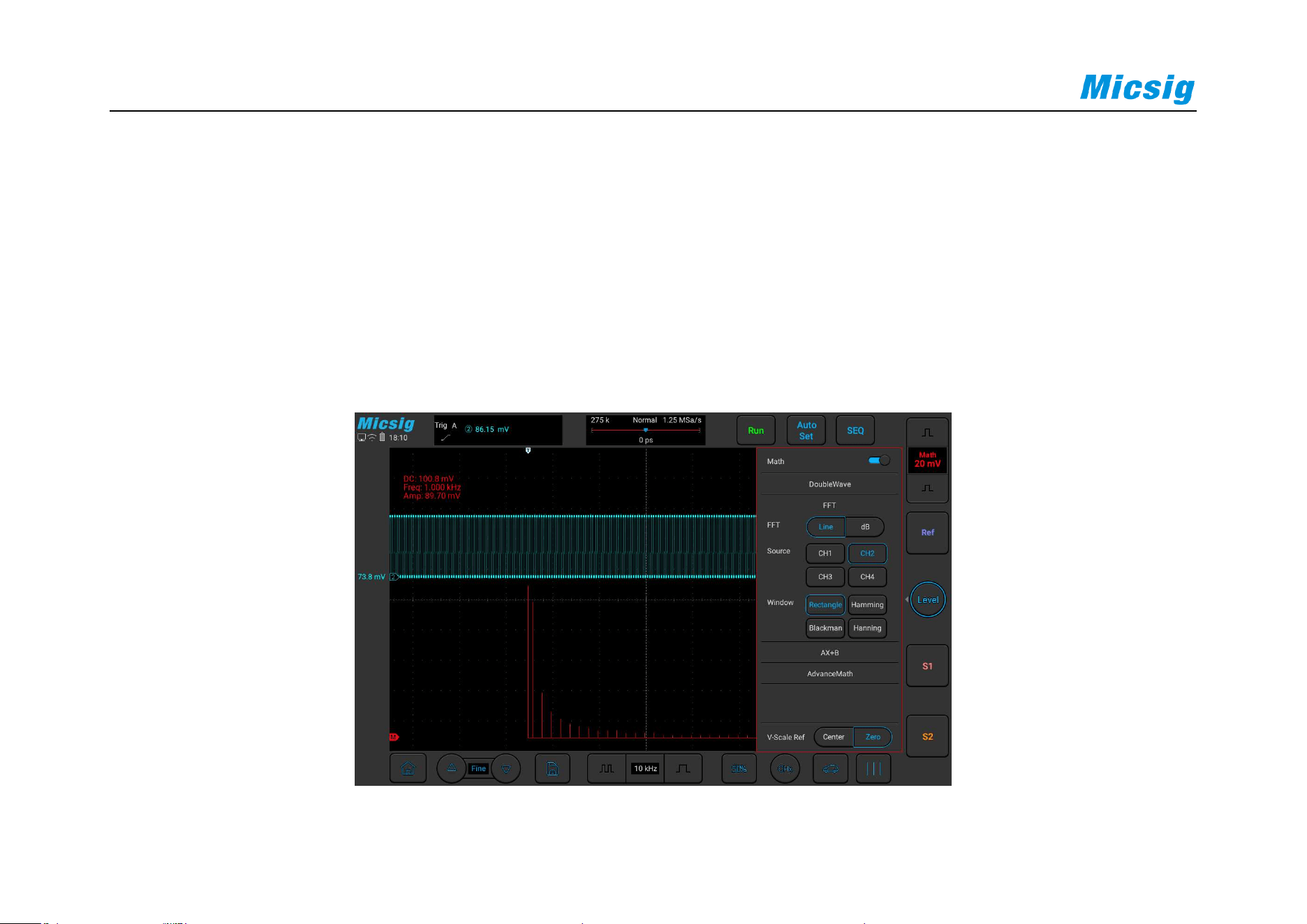
266
9.2 FFT Measurement
FFT is used to calculate the Fast Fourier Transform using the analog input channel. FFT record specifies the
digitization time of the source and converts it to the frequency domain. After selecting the FFT function, FFT
spectrum is plotted as amplitude in V-Hz or dB-Hz on the oscilloscope display screen. The reading of the horizontal
axis changes from time to frequency (Hz), while the unit of the vertical axis changes from volt to V or dB.
Figure 9-3 FFT Window

Chapter 9 MATH and Reference
267
Open FFT
1) Swipe up or down at the channel selection area to enter the second channel selection area. Tap the soft key
to open the math channel, left swipe to open math channel menu.
2) Tap spectrum type “Line/Decibel” to open the FFT window (see Figure 9-3 FFT Window).
3) Tap the Operation Source box to select the channel for which FFT transform is required.
4) Tap the window box to select the window function applied to the FFT input signal.
Selection of window function
In the FFT transform, four different FFT windows can be selected.
Each window is alternatively used between frequency resolution and amplitude accuracy, and the appropriate
window may be selected according to the characteristics of the following windows.

268
Rectangular window
This is the best window type for resolution frequencies that are very close to the same value, but this type is
the least effective at accurately measuring the amplitude of these frequencies. It is the best type of
measuring the spectrum of non-repetitive signals and measuring the frequency component close to DC.
Use the “Rectangular” window to measure transients or bursts of signal levels before or after almost the
same event. Moreover, this window can be used to measure equal-amplitude sine waves with very close
frequencies and wideband random noises with relatively slow spectral variations.
Hamming window
This is the best window type for resolution frequencies that are very close to the same value, and the
amplitude accuracy is slightly better than the “Rectangular” window. The Hamming type has a slightly
higher frequency resolution than the Hanning type.
Use Hamming to measure sinusoidal, periodic, and narrowband random noises. This window is used for
measuring transients or bursts of signal levels before or after events with significant differences.

Chapter 9 MATH and Reference
269
Hanning window
This is the best window type for measuring amplitude accuracy but less effective for resolving frequencies.
Use Hanning to measure sinusoidal, periodic, and narrowband random noises. This window is used for
measuring transients or bursts of signal levels before or after events with significant differences.
Blackman-Harris window
This is the best window type for measuring frequency amplitude, but worst for measuring the resolution
frequency.
Use the Blackman-Harris measurement to find the main single-signal frequency waveform for higher
harmonics.
Since the oscilloscope performs FFT transform on the finite-length time record, the FFT algorithm assumes
that YT waveform is continuously repeated. Thus, when the period is integral, the amplitudes of YT
waveform at the beginning and at the end are the same, and waveform will not interrupt. However, if the
period of YT waveform is not integral, the waveform amplitudes at the beginning and at the end are

270
different, resulting in high-frequency transient interruption at the junction. In the frequency domain, this
effect is called leakage. Therefore, to avoid leakage, the original waveform is multiplied by a window
function, forcing the values at the beginning and at the end to be zero.
Note: Signals with DC components or deviations can cause errors or deviations in the FFT waveform components.
AC coupling can be selected to reduce DC components.
Spectrum type
Select Line, the vertical axis reads V or A; select dB, the vertical axis reads dB. When the spectrum is linear, the
waveform is shown in Figure 9-4.
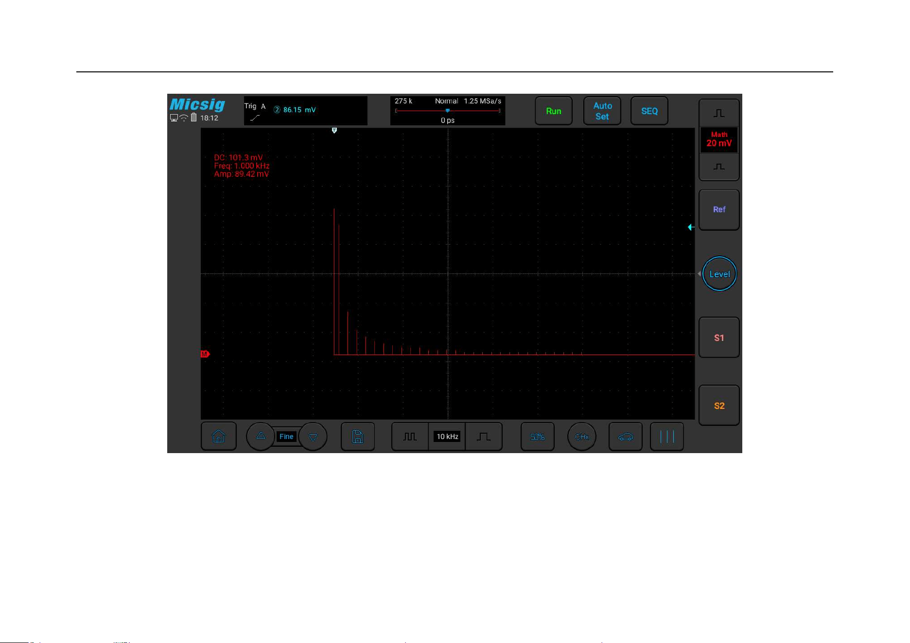
Chapter 9 MATH and Reference
271
Figure 9-4 Spectrum Amplitude as V-Hz
Adjust FFT waveforms
Waveform position

272
Select math channel as the current channel. After touching math waveform on the screen with one finger,
adjust the waveform display position by dragging upward and downward, leftward and rightward, or tap
the fine adjustment button in the lower left corner of the screen for fine adjustment
Select math channel as the current channel and press the “position” knob in the horizontal button area to
move the leftmost side of the waveform (0Hz) to the horizontal center of the screen.
Select math channel as the current channel and press the “position” knob in the vertical button area to move
the waveform to the vertical center of the screen.
Horizontal time base scale
Select math channel as the current channel, tap the time base adjustment button, and adjust the horizontal time base
scale. The horizontal time base is stepped in 1-2-5, and the waveform changes either.
For FFT measurement, the reading of the horizontal axis changes from time to frequency (Hz), and it no longer
shares the same time base with other analog channels. Therefore, before adjusting the horizontal frequency scale,
the math channel must be set as the current channel.

Chapter 9 MATH and Reference
273
Vertical sensitivity
Tap or on the right side of the screen to set the vertical sensitivity (V/div or dB/div) for the channel so
that waveform is displayed on the screen at an appropriate size. The vertical sensitivity factor is stepped in 1-2-5
(using 1:1 probe).
Note: FFT waveform does not support automatic parameter measurement.
9.3 Advanced Math
ATO series oscilloscopes support user-defined editing formulas for waveform calculation. Support the input of
functions, operators, channels, constants, variables, etc. The expression supports up to 36 characters.
Click the corresponding button to input and edit the waveform (please click in order, the ones that are grayed out
cannot be clicked).
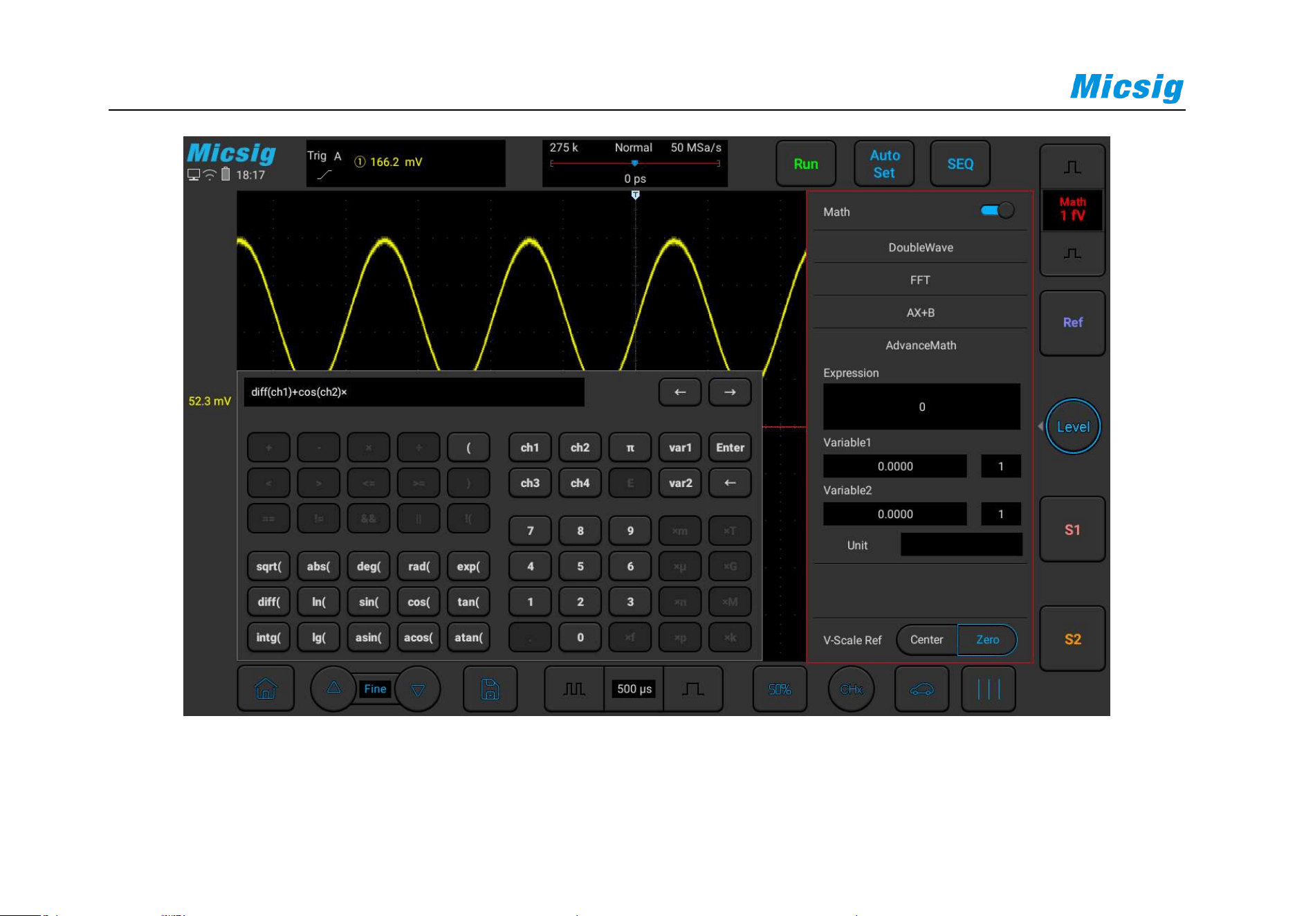
274
Figure 9-5 Advanced Math

Chapter 9 MATH and Reference
275
Type
Description
Item
Remark
Function
Sqrt()、Abs()、Deg()、
Rad()、Exp()、Diff()、
ln()、Sine()、Cos()、
Tan()、Intg()、Log()、
arcsin()、arccos()、
arctan()
Functions can be nested
Channel
Source
Ch1、Ch2、Ch3、Ch4
Variable
Source
variable1、variable2
When a variable is written in the
expression, the input box of the
variable appears in the math menu,
indicating that it can be input; for
example, input 4.1235 -3 for variable
1, which means 4.1235×9-
3

276
Variable value range -9.9999~9.9999,
variable power range -9~9
Operator
+、-、*、/、==、!=、>、
<、≥、≤、&&、||、!(
symbol
brackets
(、)
Value
Source
0、1、2、3、4、5、6、7、8、
9、.、π、E
Source
10
×
Numerical
unit
f、p、n、u、m、K、M、G、T
Table 9-2 List of Advanced Math
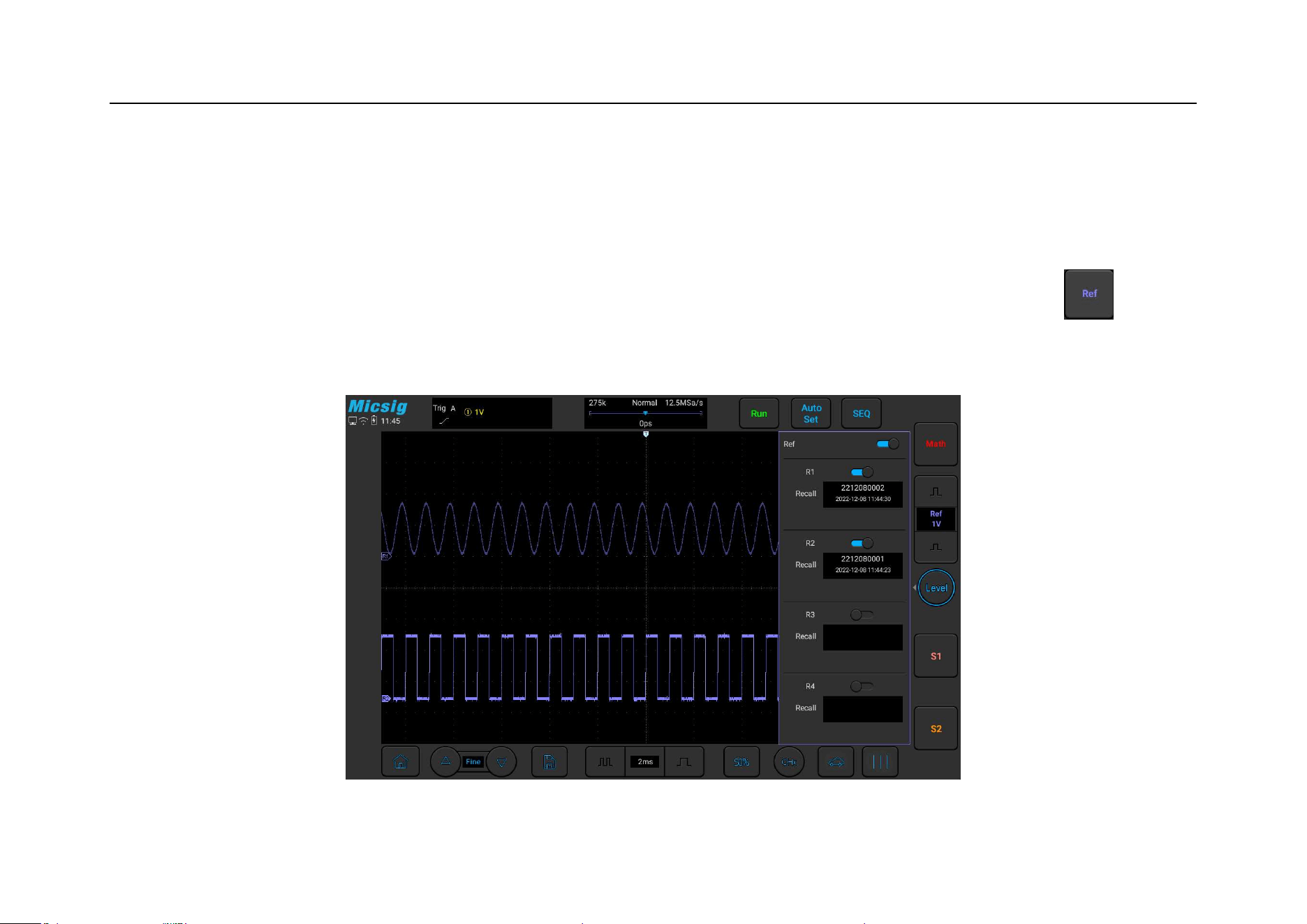
Chapter 9 MATH and Reference
277
9.4 Reference Waveform Call
Reference waveform call and close
Swipe up or down at the channel selection area to enter the second channel selection area. Left swipe button
to open the reference menu, see Figure 9-5.
Figure 9-6 Reference Channel Menu

278
When there are already waveforms loaded into the reference channel, click “Open/Close” button to open or close
the reference channel; the reference waveform is displayed in blue-violet, and the four stored waveforms can be
displayed simultaneously, wherein the current reference waveform is brighter than non-current reference
waveforms.
When there are no waveforms loaded into the reference channel, turn on the “Call” switch to call waveforms.
Take R1 as an example, with operation steps as follows:
1) Open reference menu.
2) Tap the “Call” file box under R1 to open the reference file column.
3) Click the name of the reference waveform file to be called. The file is loaded into R1 channel. Then, R1
channel is turned on as the current channel waveform, and the reference waveform channel icon is
highlighted. The displayed state changes from “Close” to “Open”. As in Figure 9-6, the brighter reference
waveform is shown as the current reference channel.
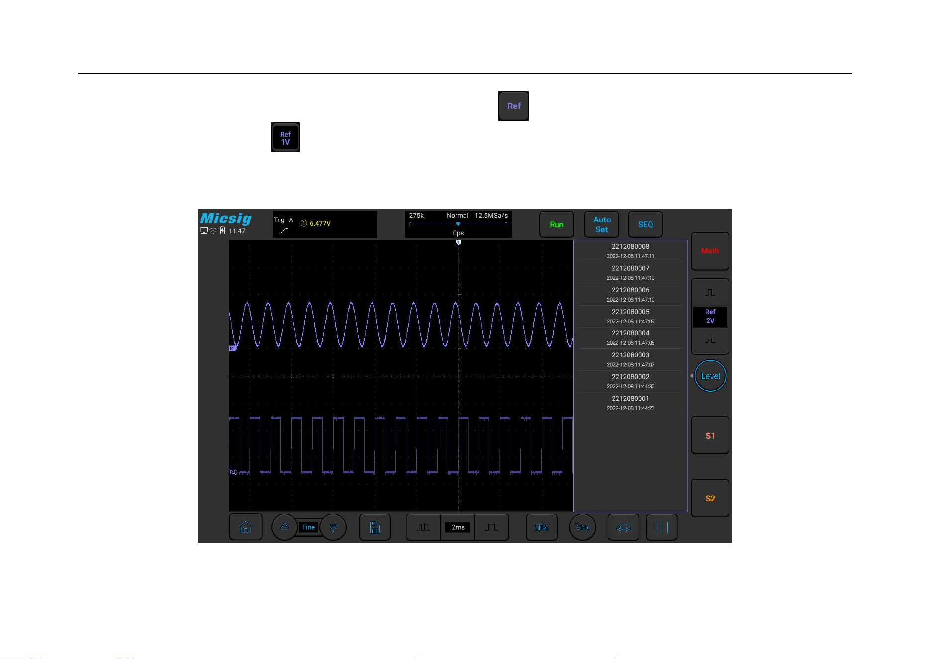
Chapter 9 MATH and Reference
279
If there are already files loaded into the reference channel, tap to open the reference channel of all loaded
reference files; Right swipe to close all currently opened reference waveforms. A single reference channel
may also be opened with the Open/Close button.
Figure 9-7 Restore Reference Waveform

280
Close the reference waveform:
1) In the reference menu, tap “Open/Close” button in R1 to close the reference waveform.
2) Repeat step 1 to close other reference channels.
3) Right swipe to turn off all reference waveforms.
Reference waveform movement and time base adjustment
The horizontal or vertical movement and zoom of reference waveforms are independent of analog channels, and the
adjustments among different reference waveform channels are also independent of each other.
To adjust the reference waveform of a channel, first set the channel as the current channel, and then adjust the
reference waveform by move or zoom (in accordance with the analog channel method).
The scale and time base of the current channel reference waveform are displayed on the reference button. After
switching the current reference channel, the scale and time base on the reference button change with the change of
current reference channel.

Chapter 10 Display Settings
281
Chapter 10 Display Settings
This chapter contains the detailed information of the display settings and function buttons of the oscilloscope. You
are recommended to read this chapter carefully to understand the display setting functions and operations of the
ATO series oscilloscope.
Waveform setting
Persistence setting
Graticule setting
Horizontal expansion center
Color temperature setting
Time base mode selection
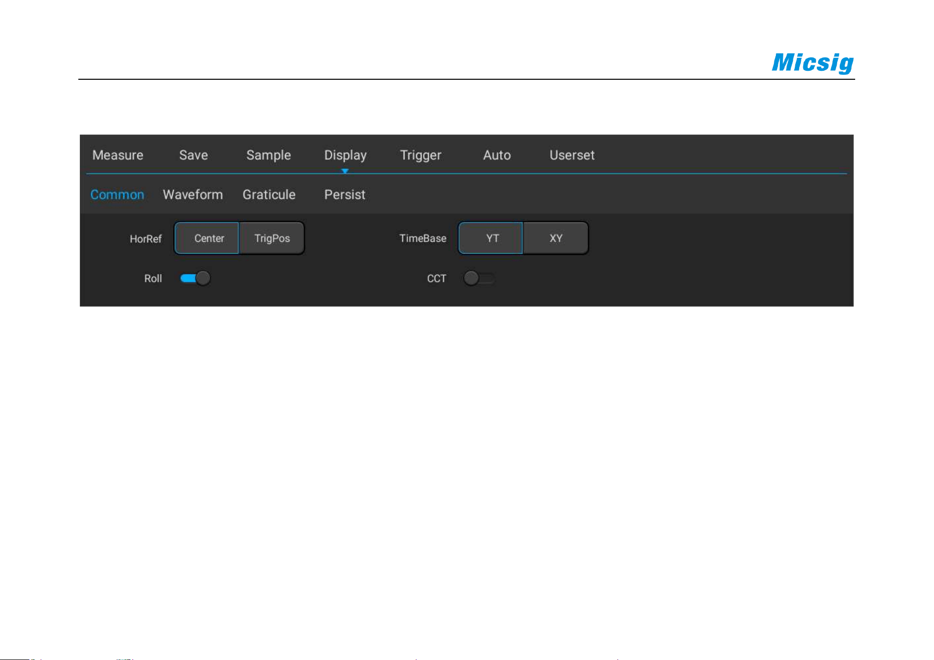
282
In the main menu, tap Display button to enter display settings menu, as shown in Figure 10-1.
Figure 10-1 Display Settings and Function Buttons
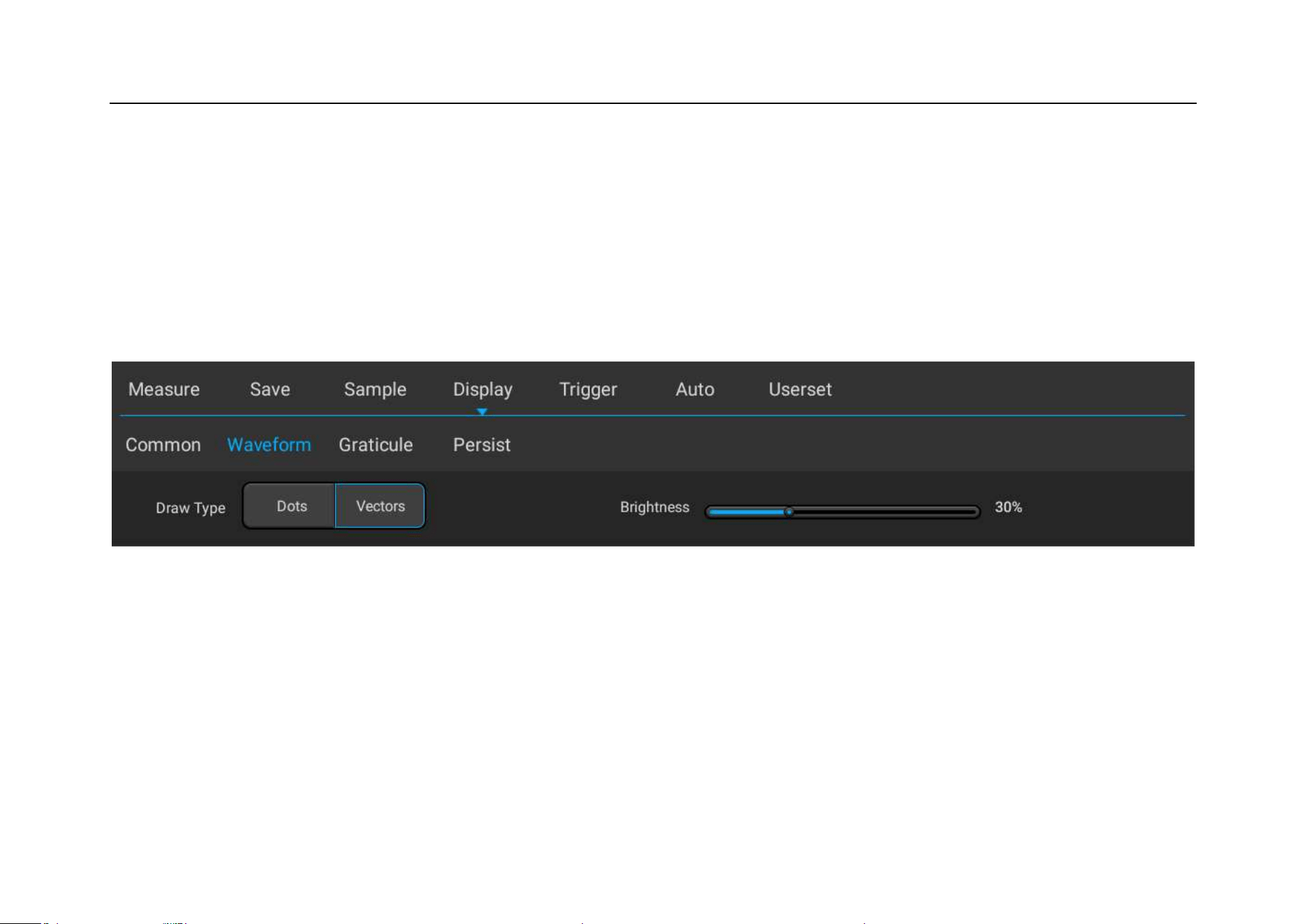
Chapter 10 Display Settings
283
10.1 Waveform Settings
Open the display menu, tap Waveform button to open the waveform display menu. This menu is used to set the
display mode and brightness of waveform. The waveform display mode is divided into two types: dots and vectors.
The waveform brightness percentage is adjustable, and the waveform display setting is shown in Figure 10-2.
Figure 10-2 Waveform Display Menu
10.2 Graticule Setting
Open the display menu and tap Graticule button to open the graticule setting menu (Figure 10-3). Graticule display
mode includes: “Full”, “Grid”, “Crosshair” and “Frame”, and the brightness percentage is adjustable.
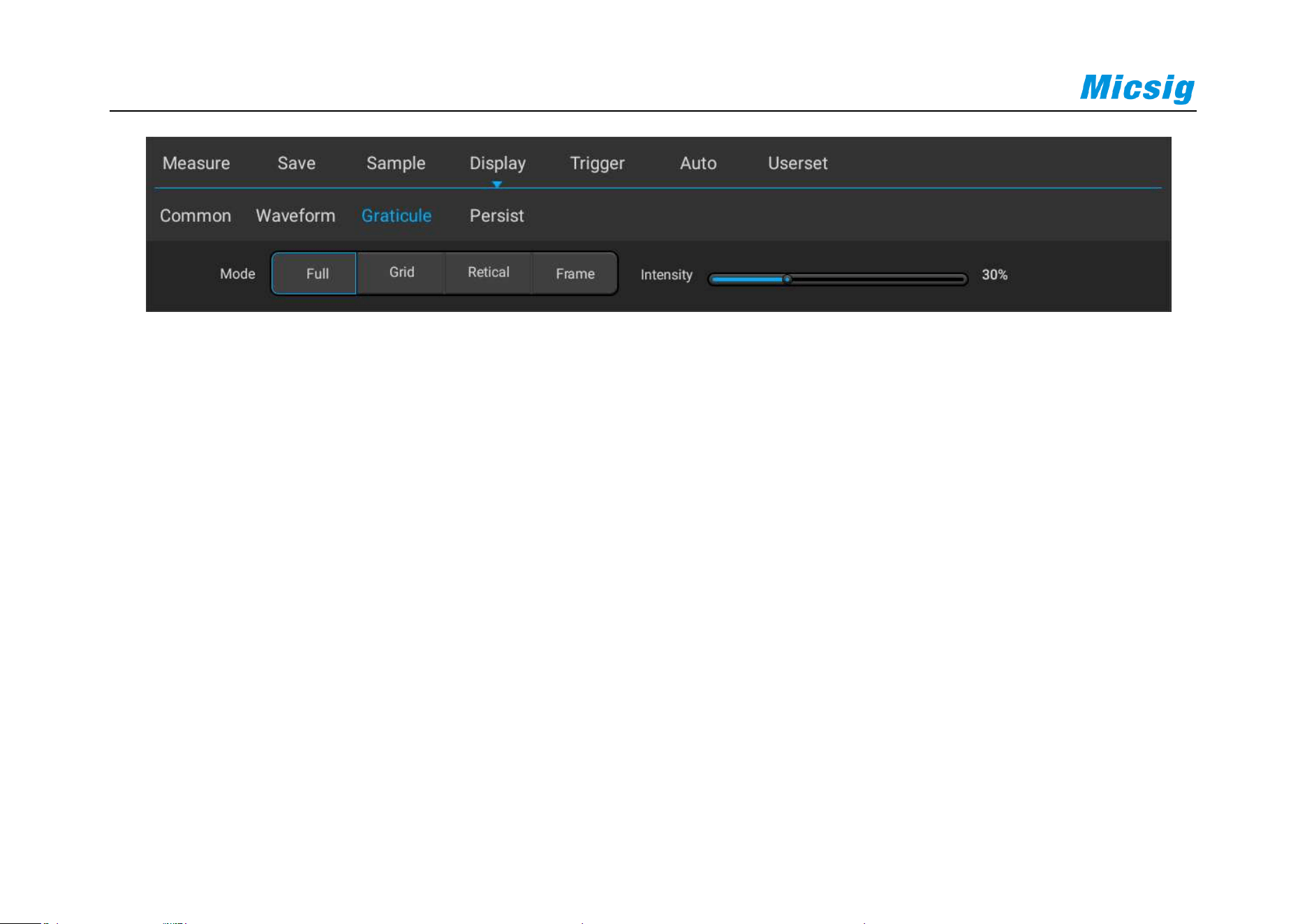
284
Figure 10-3 Graticule Menu Display
10.3 Persistence Setting
Open the display menu and tap Persist key to open the persistence settings menu.
1) Persistence setting
In the persistence setting menu, select:
None: None - no persistence.
Auto: Auto — automatic persistence.

Chapter 10 Display Settings
285
Normal: Normal - set the persistence time — After selecting the variable persistence, tap the box on the
right of “Adjust” to pop up the persistence time selection box (Figure 10-4) and set the persistence time. It
can be set between 10ms and 10s.
∞: Infinite persistence - never erase the results of previous acquisitions
Infinite persistence can be used to measure noise and jitter, display the worst-case extremes of varying
waveforms, find time violations, capture events that occur infrequently.
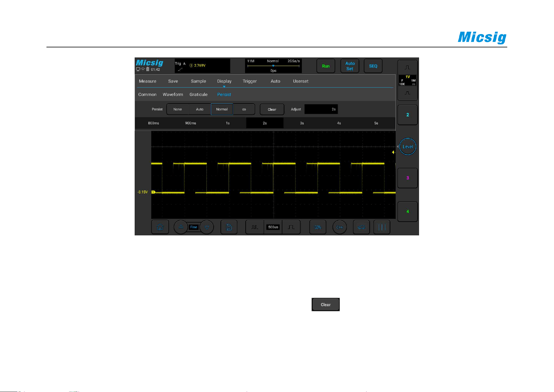
286
Figure 10-4 Persist time adjust
2) Erase persistence
To erase the previously acquired results from the display, tap key or adjust the horizontal time base
and vertical sensitivity. The oscilloscope will erase the persistence display and start the cumulative acquisition
again.

Chapter 10 Display Settings
287
10.4 Horizontal Expansion Center
Horizontal expansion is divided into two types: screen center and trigger position:
1) Screen center
Select "Center" to adjust the time base waveform to expand or contract toward both sides with the screen
center as the base point, and the delay time does not change.
2) Trigger position
Select "TrigPos" to adjust the time base waveform to expand or contract toward both sides with the trigger
position as the base point. The delay time varies with the horizontal time base.
10.5 Color Temperature Setting
Turn on the color temperature mode, and the waveform display is shown in Figure 10-5;
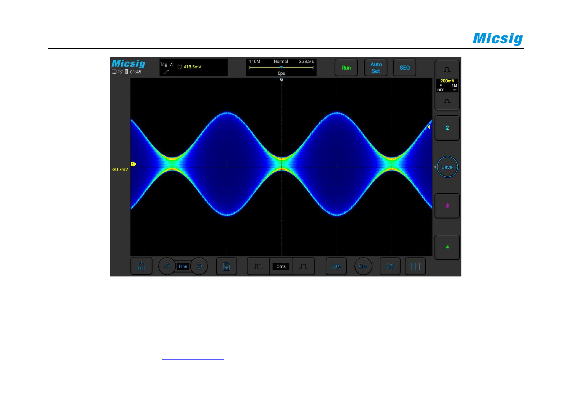

Chapter 11 Sampling System
289
Chapter 11 Sampling System
This chapter contains the detailed information of the sampling system of the oscilloscope. You are recommended to
read this chapter carefully to understand the setting and operation of the sampling system of the ATO series
oscilloscope.
Sampling overview
Run, stop and single sequence acquisition (running control)
Select sampling mode
Record length and sampling rate

290
11.1 Sampling Overview
To understand the sampling and sampling modes of the oscilloscope, you need to understand the sampling
principle, aliasing, oscilloscope bandwidth and sampling rate, oscilloscope rise time, required oscilloscope
bandwidth, and the influence of memory depth on the sampling rate.
Sampling principle
According to the Nyquist sampling principle, for a bandwidth-limited signal with the maximum frequency f
MAX
, the
equidistant sampling frequency f
S
must be twice as large as the maximum frequency f
MAX
, so that a unique signal
can be reconstructed without aliasing.
Aliasing
Aliasing occurs when the signal is under sampled (f
S
<2f
MAX
). Aliasing is signal distortion caused by incorrectly
reconstructing low frequencies from a small number of sampling points.
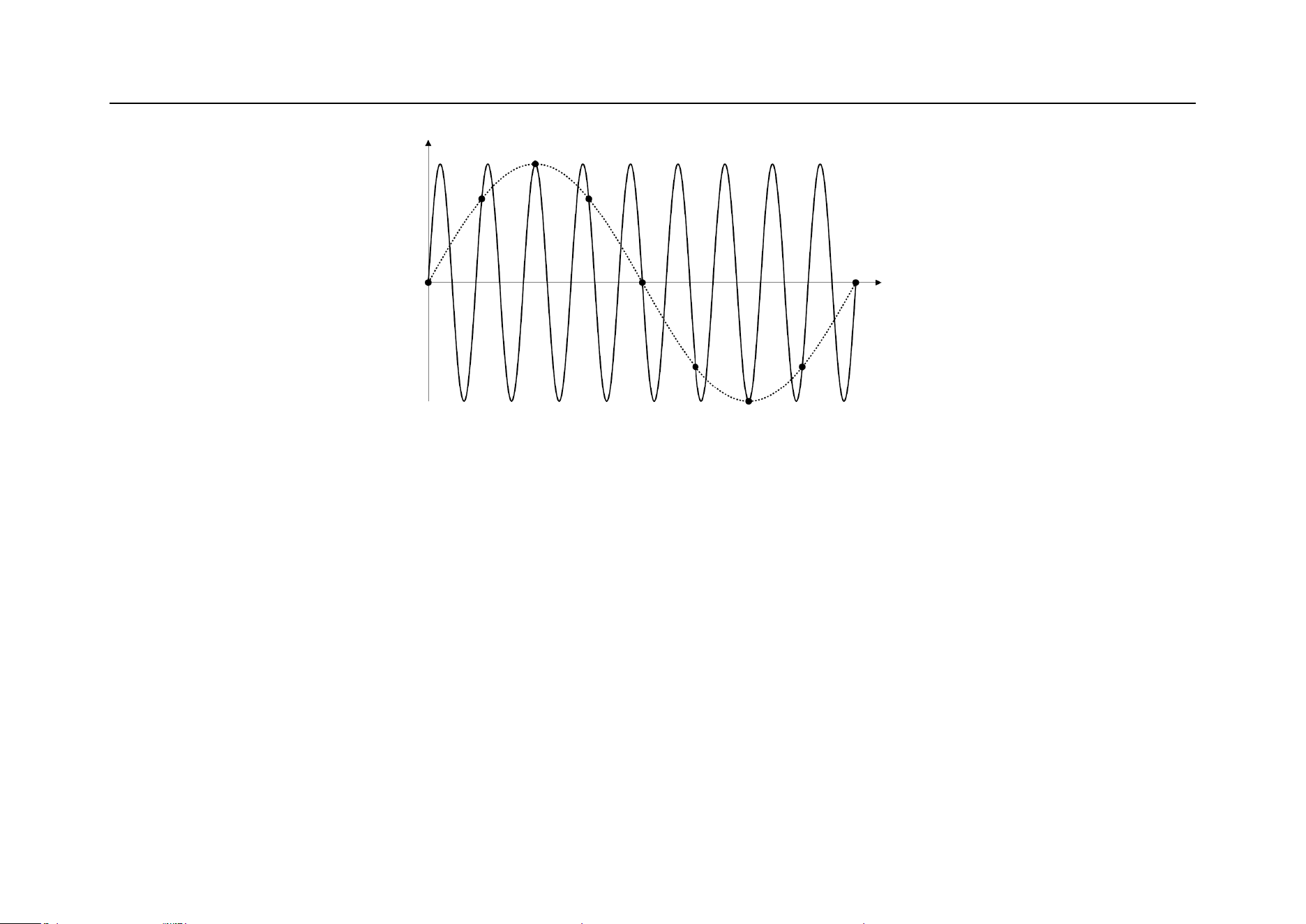
Chapter 11 Sampling System
291
Figure 11-1 Aliasing
Oscilloscope bandwidth and sampling rate
The oscilloscope bandwidth usually refers to the lowest frequency at which the input signal sine wave is attenuated
by 3dB (-30% amplitude error).
For oscilloscope bandwidth, according to the sampling principle, the required sampling rate is f
S
=2f
BW
. However,
this principle assumes that there is no frequency component exceeding f
MAX
(f
BW
in this case) and requires a system
with ideal brick-wall frequency response.
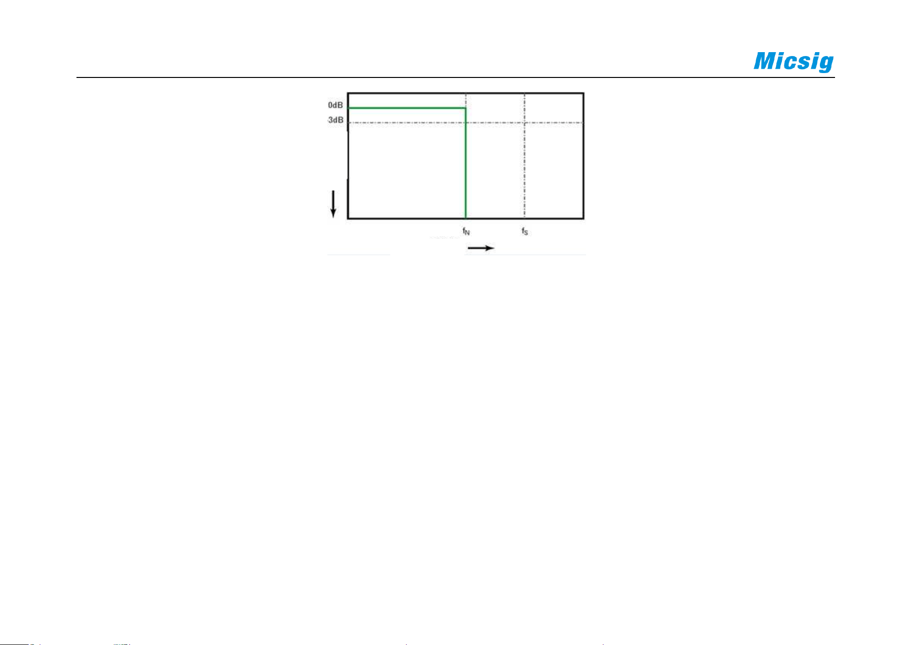
292
Figure 11-2 Theoretical Brick-Wall Frequency Response
However, digital signals have frequency components that exceed the fundamental frequency (the square wave
consists of sine waves at fundamental frequency and an infinite number of odd harmonics), and for bandwidths of
500MHz and below, the oscilloscope typically has Gaussian frequency response.
Frequency
Attenuation
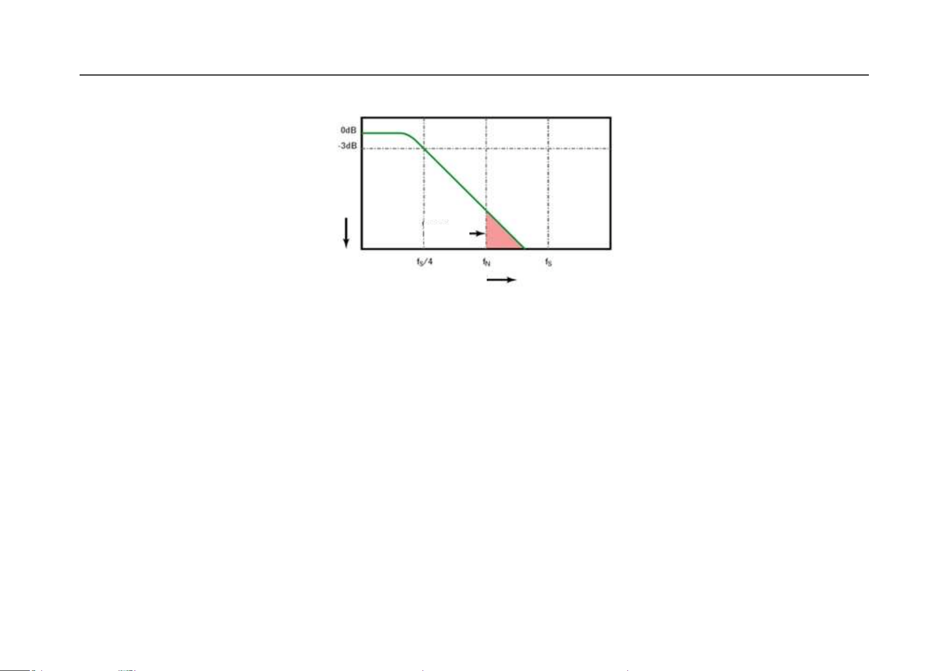
Chapter 11 Sampling System
293
Figure 11-3 Sampling Rate and Oscilloscope Bandwidth
The oscilloscope bandwidth is limited to 1/4 sampling frequency and reduces the frequency response above the
Nyquist frequency.
Therefore, in fact, the oscilloscope sampling rate should be 4 times or more of its bandwidth: f
S
≥4f
BW
. This can
reduce aliasing and cause greater attenuation in the aliased frequency components.
Frequency
Attenuation
Aliasing

294
Oscilloscope rise time
The oscilloscope rise time is closely related to its bandwidth. The rise time of an oscilloscope with Gaussian type
frequency response is approximately 0.35/f
BW
(based on the standard from 10% to 90%).
The oscilloscope rise time is not the fastest edge speed that an oscilloscope can accurately measure. It is the fastest
edge speed that the oscilloscope can produce.
Desired oscilloscope bandwidth
The oscilloscope bandwidth required to accurately measure signal is primarily determined by the rise time of the
signal rather than the frequency of the signal.
The following steps can be used to calculate the required oscilloscope bandwidth:
1) Determine the fastest edge speed.
Rise time information is typically obtained from the published device specifications used in the design.
2) Calculate the maximum “actual” frequency component.

Chapter 11 Sampling System
295
According to Dr. Howard W. Johnson’s book “High-Speed Digital Design–A Handbook of Black Magic”, all
fast edges have wirelessly continuous frequency components. However, there is a turning point (or “inflection
point”) in the fast edge spectrum at which frequency components above f
knee
are negligible in determining the
signal shape.
f
knee
=0.5/signal rise time (based on 10% - 90% threshold)
f
knee
=0.4/signal rise time (based on 20% - 80% threshold)
3) The multiplication factor for the desired accuracy is used to determine the required oscilloscope bandwidth.
Desired
Accuracy
Desired Oscilloscope
Bandwidth
20%
f
BW
=1.0xf
knee
10%
f
BW
=1.3xf
knee
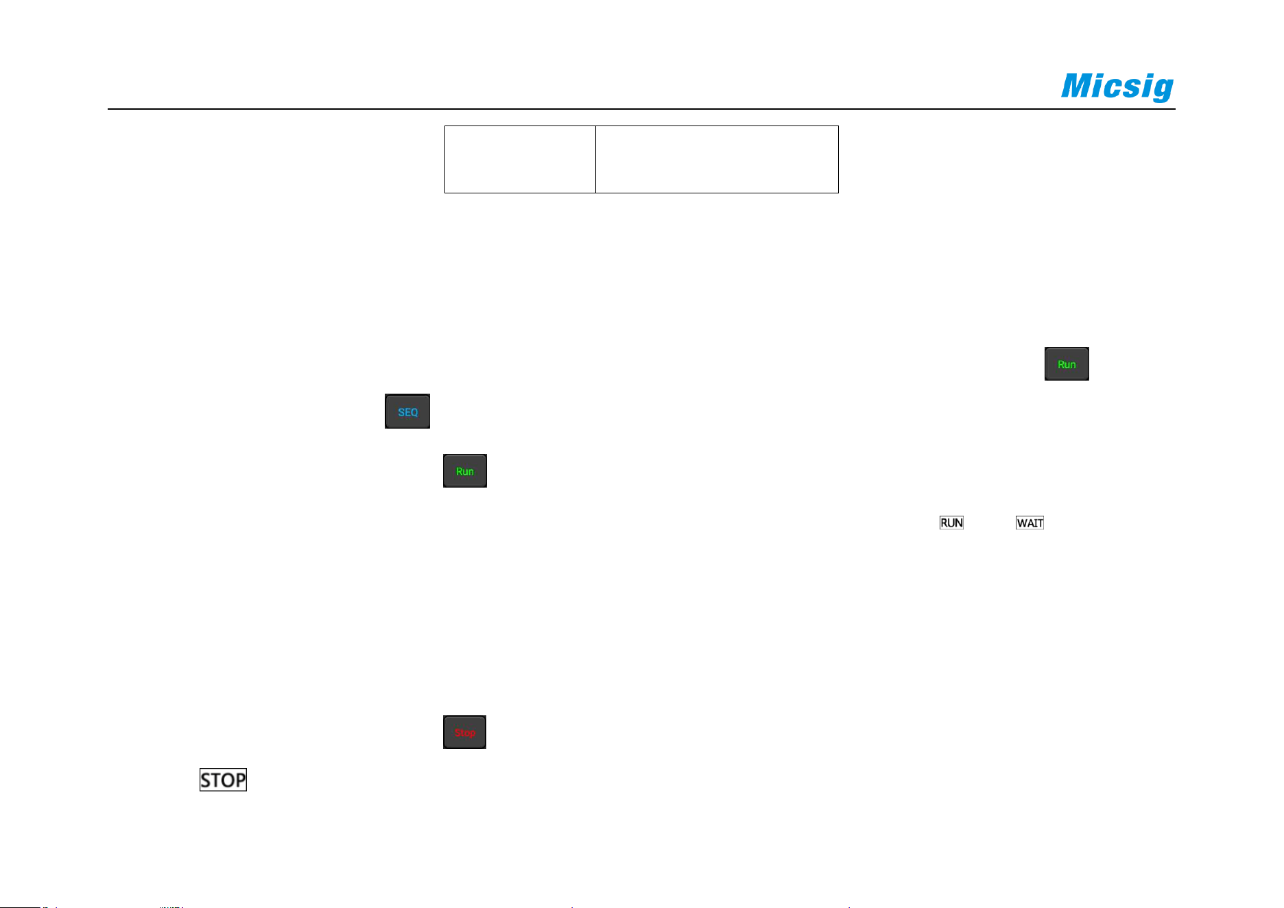
296
3%
f
BW
=1.9xf
knee
Figure 11-4 Bandwidth Corresponding to Oscilloscope Measurement Accuracy
11.2 Run/Stop Key and Single SEQ Key
Use softkeys in the button area to start and stop the oscilloscope acquisition system: Run/Stop button and
Single Sequence Acquisition button.
When the Run/Stop button is displayed in green, it indicates that the oscilloscope is running, that is,
it meets the trigger condition and data acquisition is being performed. The green “ ” or “ ” is displayed
in the upper left corner of the screen.
To stop data collection, tap the Run/Stop button. After stopping, the screen displays the last acquired
waveform.
When the Run/Stop button is displayed in red, it indicates that data acquisition has stopped. The red
“ ” is displayed in the upper left corner of the screen.

Chapter 11 Sampling System
297
To resume data acquisition, press the Run/Stop button again.
To capture and display single acquisition (whether the oscilloscope is running or stopped), tap the single
sequence key for a single acquisition.
11.3 Select Sampling Mode
Open the main menu, tap the sampling mode option under “Sampling”, and choose among the four sampling
modes: normal, average, peak and envelope in the pop-up box.
The sampling modes of all channels are same. That is, if the sampling mode of any channel is changed, the
sampling mode of all channels is changed at the same time.
Normal sampling mode
Oscilloscope samples signal through equivalent time intervals to build waveform. When the time base of 20 ns or
faster is chosen, the oscilloscope automatically performs an interpolation algorithm that inserts difference point
between sampling points.

298
This mode produces the best display effects for most waveforms.
Peak sampling mode
In peak sampling mode, when the horizontal time base setting is low, the minimum and maximum sample values
are retained to capture rare events and narrow events (with any noise expanded). This mode will display all pulses
that are at least as wide as the sampling period.
When the time base is set to 200ms and above, the oscilloscope will automatically exit the peak sampling mode and
switch to the normal sampling mode.
Burr or narrow pulse capture
Burr is the rapid change in waveform that is usually narrower than waveform. Peak sampling mode can be used to
view burr or narrow pulses more easily. In the peak sampling mode, narrow burr and transition edges are brighter
than in those in the “normal” sampling mode, making them easier to see.
Applying the peak sampling mode can avoid signal aliasing but show more real noises.
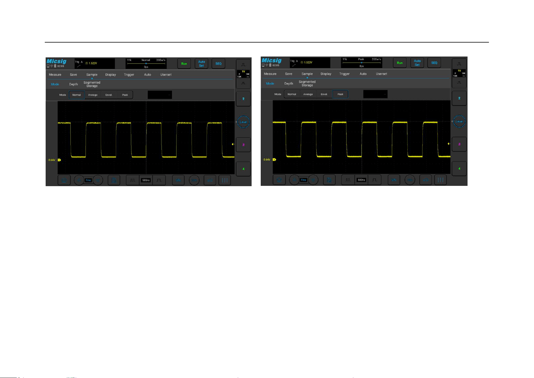
Chapter 11 Sampling System
299
Figure 11-5 Sine Wave with Burr
Normal Sampling Mode
Figure 11-6 Sine Wave with Burr
Peak Sampling Mode
Use peak detection mode to find burrs
1) Connect signal to the oscilloscope to be stably displayed.
2) To find burr, select the peak sampling mode in Sampling Mode option in the Channel menu.

300
3) In the menu, tap “Display” → “Persistence”, then tap “∞” (infinite persistence). The oscilloscope will restart
sampling data and display them on the screen.
4) Use the zoom mode to represent the characteristics of burr:
a. Tap the “Zoom” button in the main menu to open the zoom window.
b. To get a better resolution of burr, expand the time base to set the expanded portion of the normal window
view around burr.
Average sampling mode
The average sampling mode averages multiple acquisition results to reduce random or unrelated noises in the
displayed signal. The average of multiple sampling results requires stable trigger.
The average number can be set in the selection box after the average sampling mode, and can be set to eight order
of magnitudes: 2, 4, 8, 16, 32, 64, 128 and 256.

Chapter 11 Sampling System
301
The higher the average number is, the slower the response of the displayed waveform-to-waveform changes. A
compromise must be made between the response speed of waveform versus the changes and the degree of noise
reduction shown on the signal.
Use average sampling mode
1) Open the channel menu and select the average sampling mode in the sampling mode option.
2) Press the number box on the right of the average sampling mode box to pop up the average number and then
tap it to set the average number that can best eliminate displayed waveform noises.
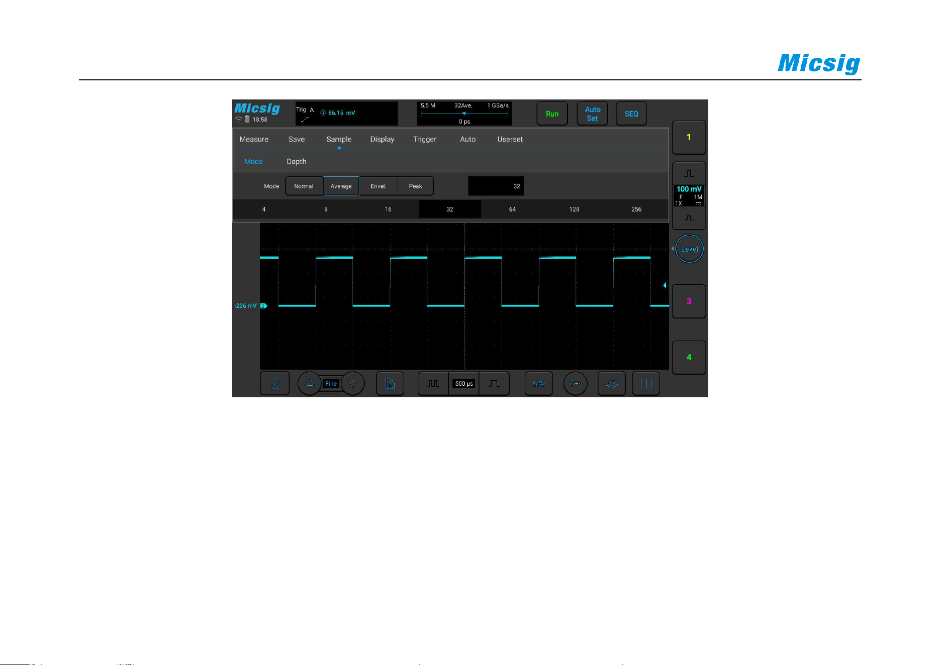
302
Figure 11-7 Waveform after choosing the average sampling mode, with average number 32
Envelope sampling mode
In the envelope sampling mode, the superposition effect of several sampled waveforms can be observed. The
maximum and minimum values of one signal can be captured in the specified N sample data, and the number of
waveform superpositions can be set to 2, 4 , 8, 16, 32, 64, 128, 256 or ∞.
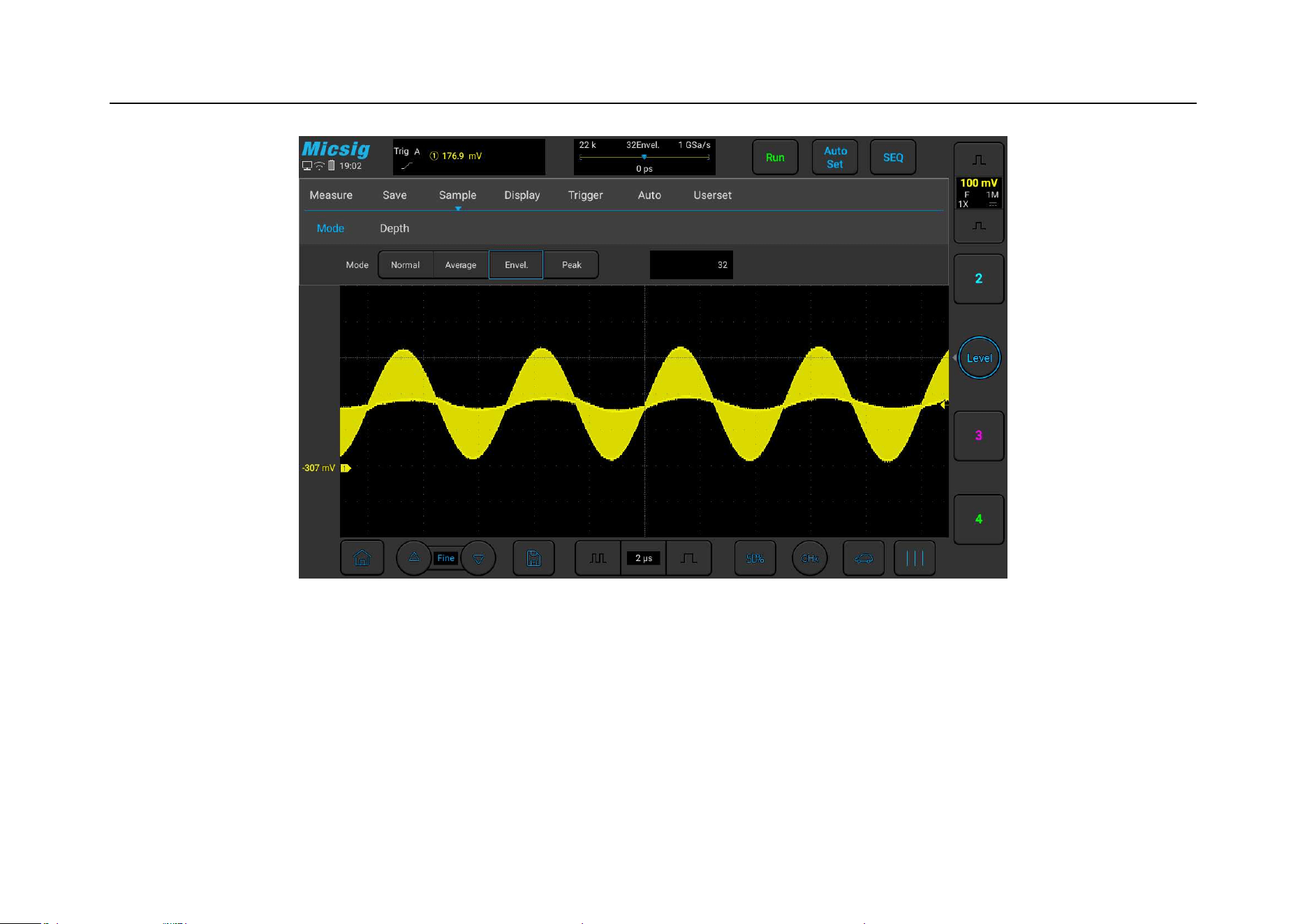
Chapter 11 Sampling System
303
Figure 11-8 AM Signal in Envelope Sampling Mode (32)
11.4 Record Length and Sampling Rate
The record length is the data volume for each captured waveform. For example, if the record length is 700K, it
means that 700K sample points are captured by one trigger.
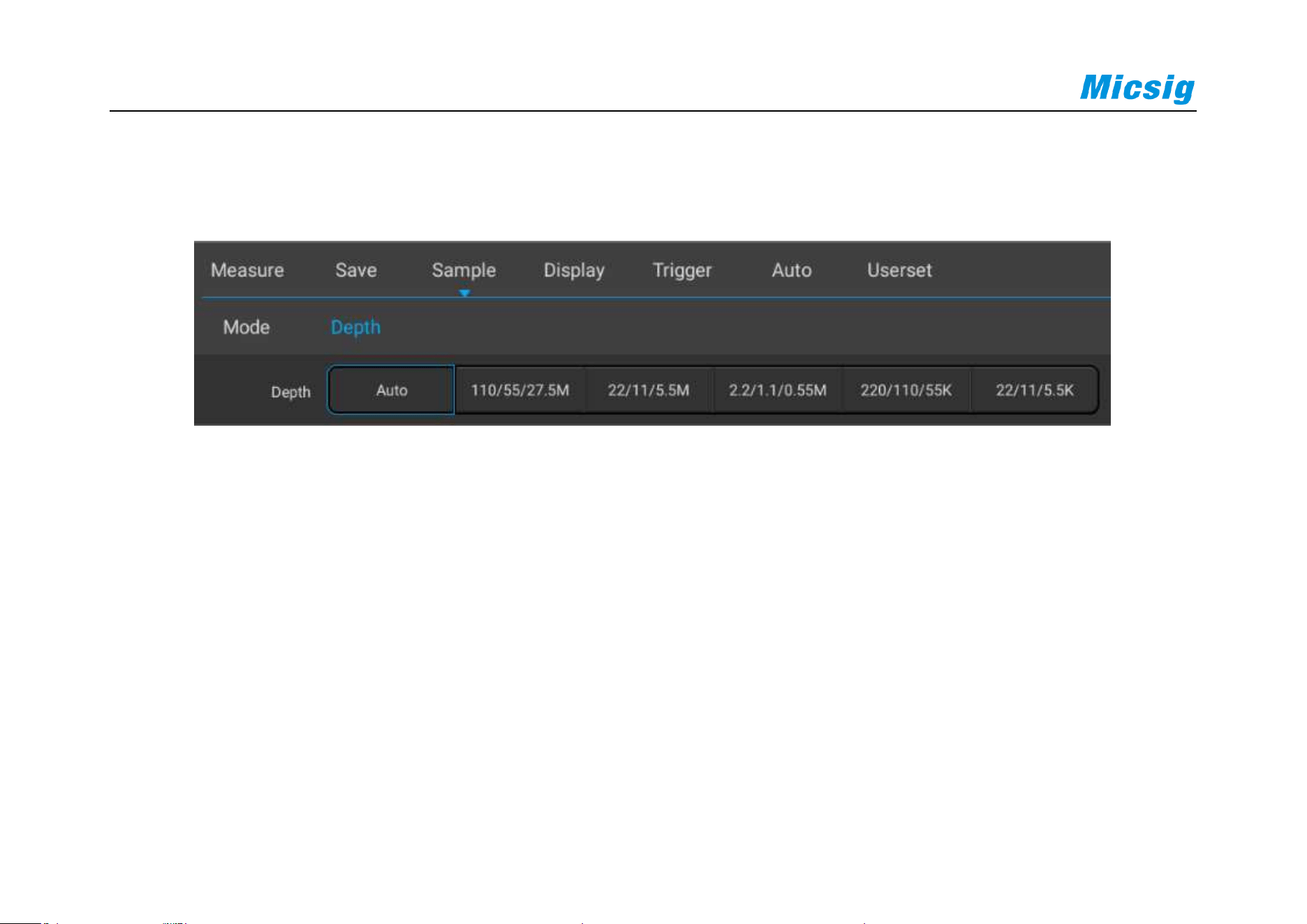
304
In the main menu, tap "Sample" to enter the record length setting menu, which can be set by tapping the
corresponding record length.
Figure 11-9 Record Length
In normal refresh mode, if it is a single channel, the record length can be set to 22k, 220k, 2.2M, 22M, 110M, Auto;
if it is dual channel, the record length can be set to 11k, 110k, 1.1M, 11M, 55M, Auto; if it is three or four channels,
the record length can be set to 5.5k, 55k, 0.55M, 5.5M, 27.5M, Auto.
Record length and sampling rate
The record length is data volume collected per waveform capture. For example, if the record length is 0.7M, it
means that 700K sample points are captured by one trigger.

Chapter 11 Sampling System
305
The oscilloscope record length and sampling rate have the following relationship:
Sampling rate = record length/acquisition time
Generally, the oscilloscope acquisition time is exactly the display time on the current entire screen (current
horizontal time base×14).
For example, if the oscilloscope has the memory depth of 700K, the sampling rate of 1GSa/s, and the horizontal
time base of 50us/div, the acquisition time is 700us, which is 50us/div×14div.
However, when the fast time base (below 20 ns) or the record length is set to a fixed value, the oscilloscope
acquisition time does not necessarily represent the display time on the current entire screen.
For example, if the oscilloscope has the memory depth of 700K, the sampling rate of 1GSa/s, and the horizontal
time base of 20ns, the acquisition time is 700ns, which is 2.5 times of the current display time on the entire screen.
Or, if the memory depth is 140K (fixed value), the sampling rate is 1GSa/s, and the horizontal time base is 1us, the
acquisition time is 140us, which is 10 times of the current display time on the entire screen.
For a single channel in a channel pair, the maximum sampling rate of the ATO series oscilloscope is 1GSa/s.

306
If any two channels are opened, the sampling rate of the two channels will halved. For example, when CH1 and
CH3 are opened, the sampling rates of CH1 and CH3 are both 500 MSa/s.
If any three channels or all four channels are opened, the sampling rate per channel will become 1/4 of the
maximum sampling rate. For example, when CH1, CH2 and CH3 are opened, the sampling rates of CH1, CH2 and
CH3 are 250 MSa/s for each of them.

Chapter 12 Serial Bus Trigger and Decode (Optional)
307
Chapter 12 Serial Bus Trigger and Decode (Optional)
This chapter contains the detailed information of serial bus decoding. You are recommended to read this chapter
carefully to understand the setting and operation of Smart bus trigger and decode.
This chapter mainly include the below contents:
UART (RS232/RS422/RS485) bus trigger and decode
LIN bus trigger and decode
CAN(FD) bus trigger and decode
SPI bus trigger and decode
I2C bus trigger and decode
ARINC429 bus trigger and decode (Optional)
1553B bus trigger and decode (Optional)

308
Swipe up or down at the channel selection area to enter the second channel selection area, tap or to
enable decoding, open bus configuration menu, select bus type, there are seven bus types: UART
(RS232/RS422/RS485), LIN, CAN(FD), SPI, I2C, ARINC429, 1553B, where channels S1 and S2 can be used for
decoding simultaneously. Open the trigger setting menu, choose an appropriate trigger type, the corresponding bus
trigger type and trigger mode can be set when the bus trigger is selected, and the serial bus is displayed in graphic
form.
In the serial bus decode mode, if it is screen rolling in other modes, the time base is automatically adjusted to 1ms
when switching to serial decode (the maximum time base supported by the serial decode mode is 100ms); in Zoom
mode, the enlarged signal can be decoded and displayed. The normal display window supports a maximum time
base of 100ms. When decoding is enabled, clicking “AUTO” will set the trigger type to be the same as the decode
channel bus type. The bus type selection menu is shown in Figure 12-1:
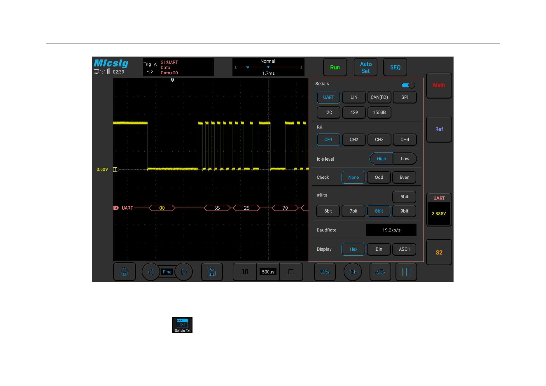
Chapter 12 Serial Bus Trigger and Decode (Optional)
309
Figure 12-1 Bus Type Selection Menu
Open the pull-up menu and tap key to open or close the text mode, as shown in Figure 12-2.
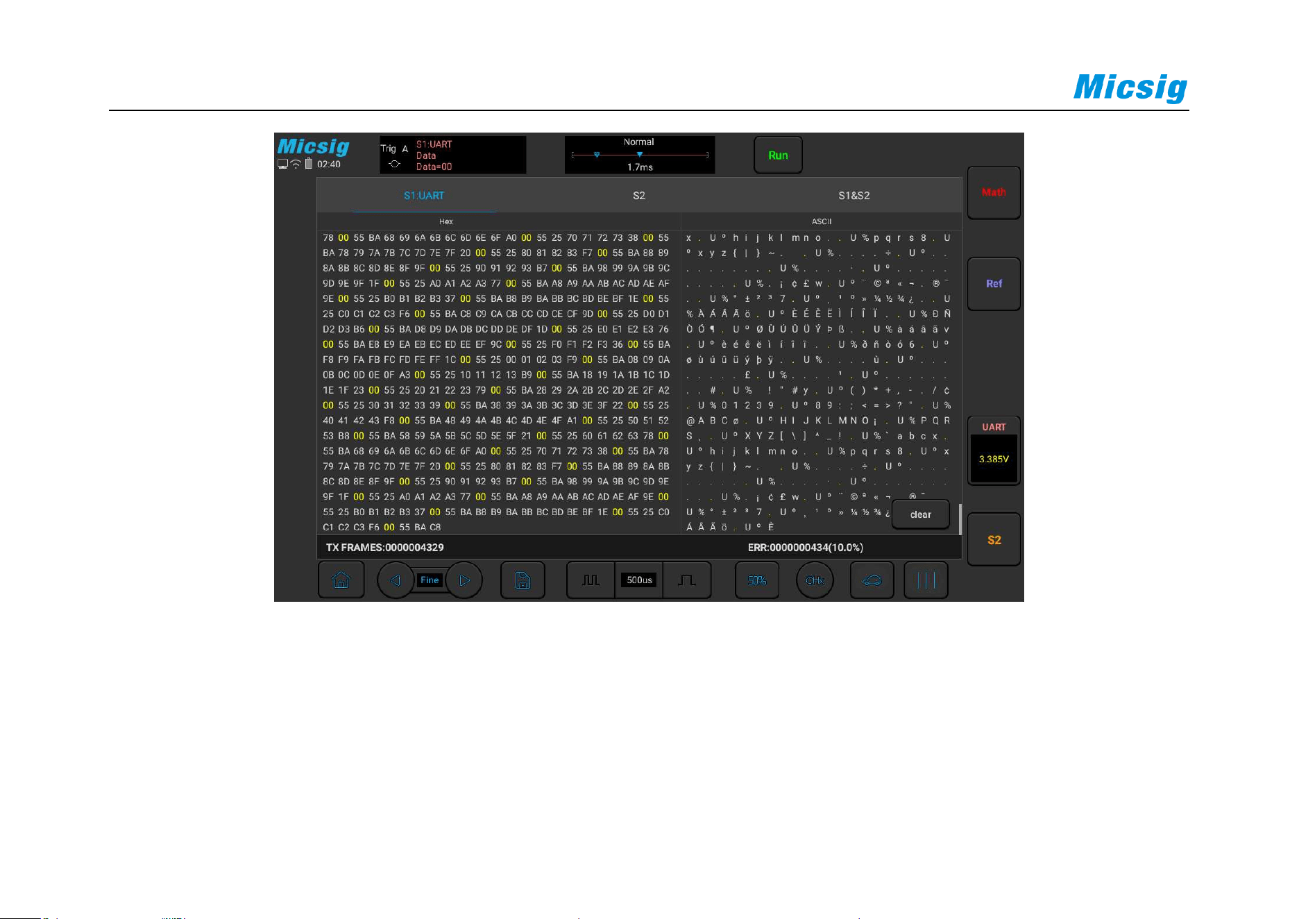
310
Figure 12-2 Bus Decode Text Mode
Description:
Two decode channels S1&S2 in the text interface must be configured identically to be opened, and each channel is
displayed in chronological order with different colors;
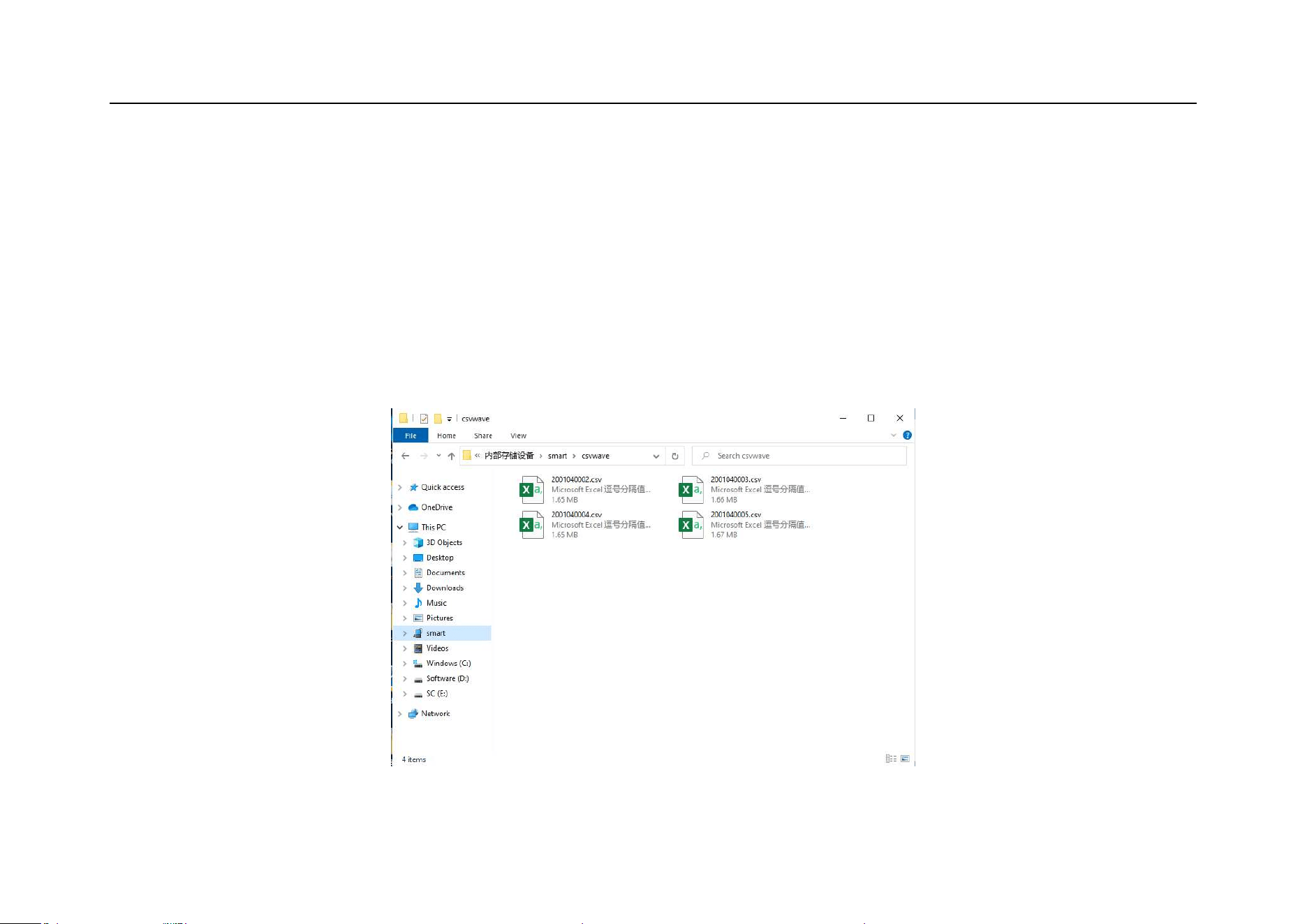
Chapter 12 Serial Bus Trigger and Decode (Optional)
311
S1/S2/S1&S2 are the channel configuration bus information, and X knob is rotated or the label is switched to
change the bus channel;
Clicking save during the text acquisition process can save all currently acquired data. If the date volume is too
large, “wait” will be displayed, and the save success prompt will be displayed.
Oscilloscope can be used as a USB storage device to view saved files on a computer, as shown in Figure 12-3:
Figure 12-3 Bus Text Storage Files

312
12.1 UART (RS232/RS422/RS485) Bus Trigger and Decode
For correctly decoding UART(RS232/RS422/RS485) bus data and making trigger stable, the bus configuration,
trigger mode setting and trigger level need to be adjusted.
Bus configuration
Left swipe or to open the bus configuration menu, as shown in Figure 12-4. The RX channel must
be chosen and the following parameters must be set according to measured signals:
Idle Level — Choose Idle Low or Idle High to match the idle state of measured equipment. For RS232, Idle
Low may be chosen.
Note: RS232 industry standard uses “negative logic”, namely high level is logic “0” and low level is logic
“1”.
Parity Bit — Choose odd, even or none depending on measured equipment.
Word Length — Set the number of bits in UART word to match measured equipment (5-9 bits available).

Chapter 12 Serial Bus Trigger and Decode (Optional)
313
Baud Rate — Choose the baud rate that matches signal in measured equipment.
The baud rate can be set within the range from 1.2Kb/S to 8.000Mb/S.
Bus Display — Choose hexadecimal, binary or ASCII code display.
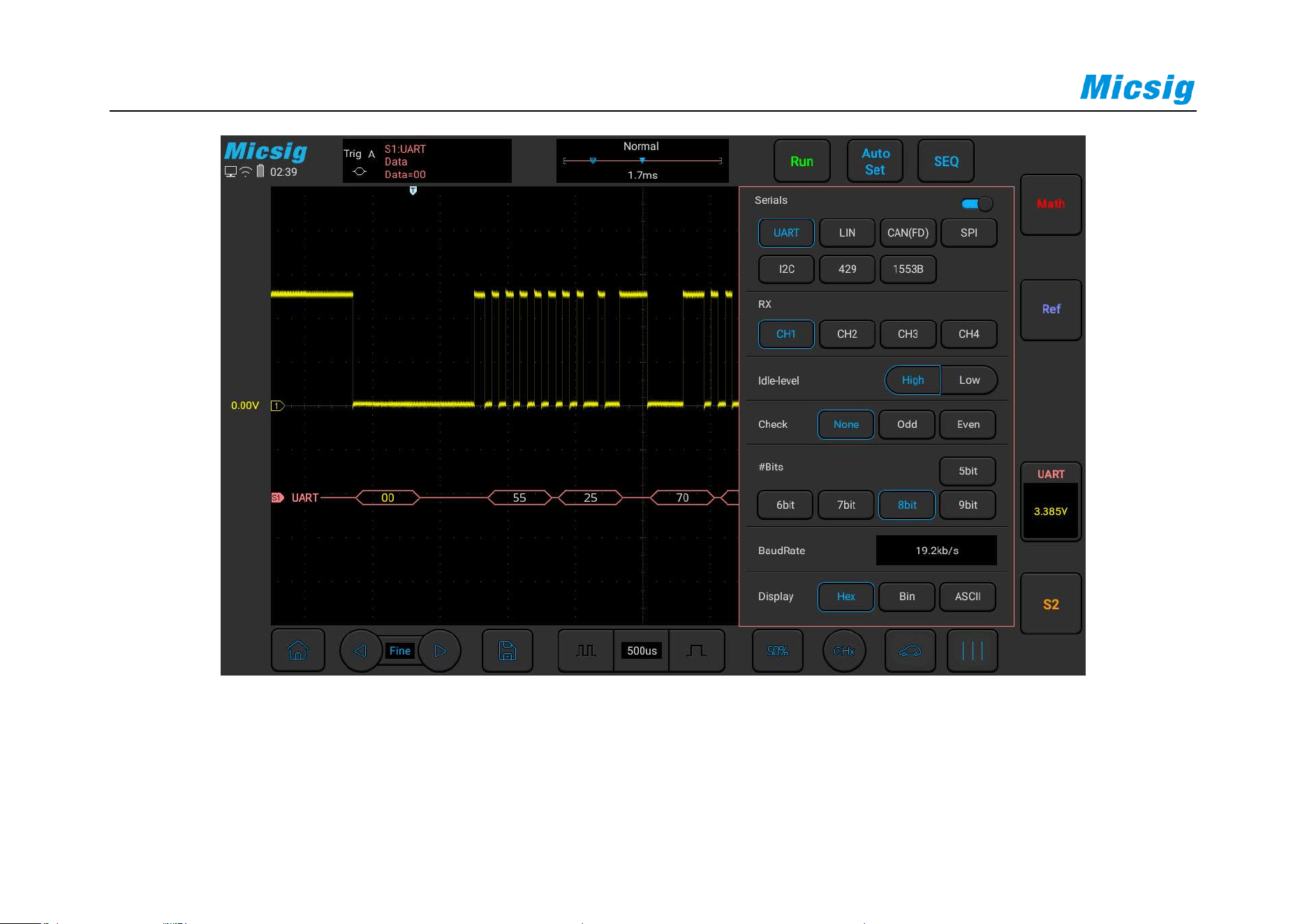
314
Figure 12-4 UART Bus Configuration Menu

Chapter 12 Serial Bus Trigger and Decode (Optional)
315
When word is displayed in ASCII, 7-bit ASCII format is used. Valid ASCII characters are between 0x00 and
0x7F. To display in ASCII, at least 7 bits in the “Bus Configuration” must be chosen. If ASCII is chosen and the
data exceeds 0x7F, the data will be displayed in hexadecimal.
Click the baud rate setting box to open the baud rate selection column. If Custom is chosen, click to pop up the
virtual soft keyboard, select the bit to be modified, enter value, and click “Enter” on the virtual soft keyboard to
complete setting. The baud rate can be set from 1.2Kb/S to 8.000Mb/S. The virtual soft keyboard is shown in
Figure 12-5:
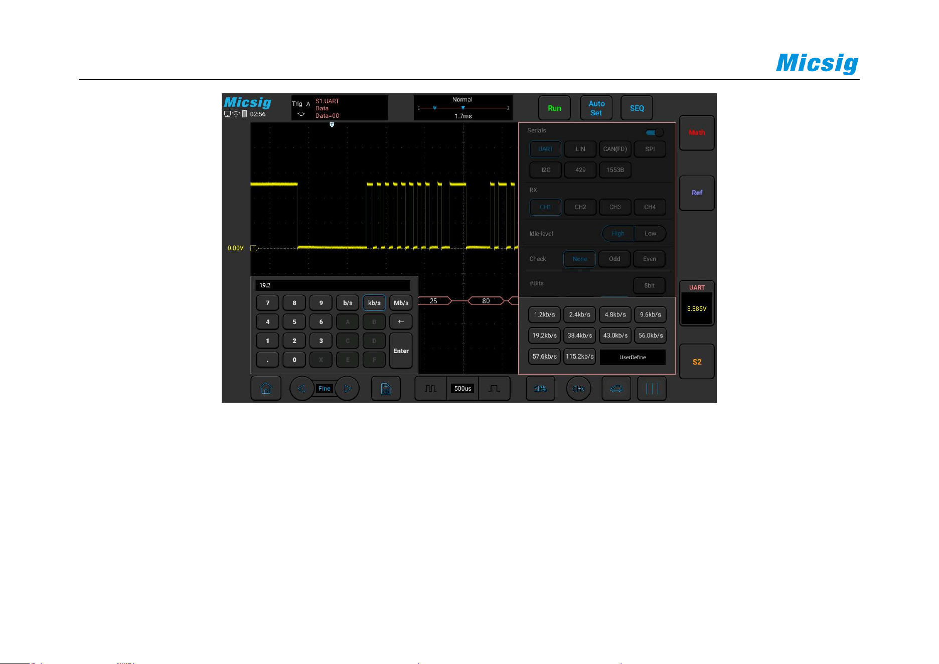
316
Figure 12-5 Baud Rate Default Setting
Note: When there is parity bit, the data word length indicates the total length of data bit plus parity bit. When
there is no parity bit, the data word length is considered to be the length of data bit. For example, if the data
word length is 8bit, when there is no parity bit, it means that the total length of data bits is 8bit; when there is
parity bit, it means that the total length of data bits is 7bit, and there is parity bit of 1 bit.
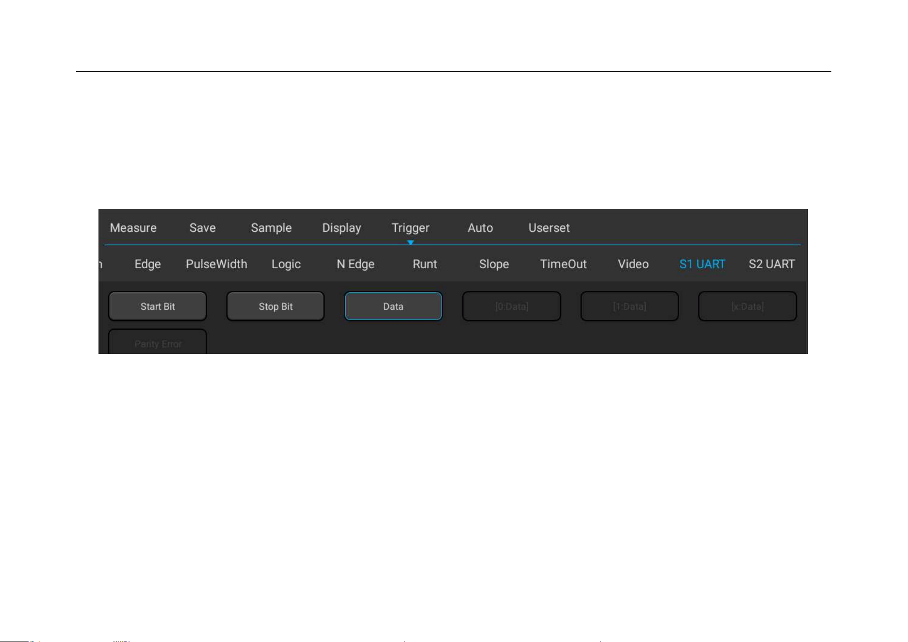
Chapter 12 Serial Bus Trigger and Decode (Optional)
317
Trigger mode
Open the trigger configuration menu and select the appropriate trigger type; when choosing UART bus trigger,
the trigger type, trigger relationship and trigger data need to be set, as shown in Figure 12-6:
Figure 12-6 Trigger Setting Menu
After selecting the trigger data, use the pop-up virtual keyboard to modify it, enter the value, and click “Enter”
on the virtual soft keyboard to complete the setting.
UART trigger configuration menu description:
a) Start bit — trigger at the start bit of the measured signal;

318
b) Stop bit — trigger at the stop bit of the measured signal, no matter the measured signal uses 1, 1.5, or 2
stop bits or not, the trigger will occur at the first stop bit.
c) [data] — Trigger at the specified data bit, when measured signal data bits are effective as 5 to 8bits, select
[data], and select the trigger relationship as “=”, “>” , “ <”, “≠”, then select “Trigger Data”, press data on
the touch screen, and use the pop-up virtual keyboard to modify;
d) [0:data] — the measured signal data bits is 9bits (the 9th bit is parity bit). Only when the 9th bit is 0, then
trigger. The trigger relationship, trigger data configuration are the same as those of [data] trigger;
e) [1:data] — the measured signal data bits is 9bits (the 9th bit is parity bit). Only when the 9th bit is 1, then
trigger. The trigger relationship, trigger data configuration are the same as those of [data] trigger;
f) [x:data] — the measured signal data bits is 9bits (the 9th bit is parity bit). No matter what the value of the
9th bit is, trigger at the designated data bit. The trigger relationship, trigger data configuration are the same
as those of [data] trigger;
g) Parity error — valid when there is parity check at parity bit, trigger while parity error.

Chapter 12 Serial Bus Trigger and Decode (Optional)
319
UART serial decode
The measured signal word length is 8bit; parity bit, none; baud rate, 19.2kb/s, hexadecimal; trigger mode as
data bit:55; follow the steps as below:
(1) Tap S1 to open the decode channel, and click S1 again to open the bus configuration menu;
(2) Select the bus type as “UART”, click “Ch1”, “Idle High”, “Parity None”, “8bit”, “19.20kb/s”, display
“hexadecimal”, then close menu;
(3) Open the trigger mode setting menu, click “Data”, enter 55 manually, and press “enter” to confirm;
(4) Adjusting the threshold level according to the amplitude level of signal may make the signal to be stably
triggered. The UART trigger graphic interface is shown in Figure 12-8:
Method 1: Click configuration information to open the decode channel threshold level adjustment
box, and drag the adjustment box upward and downward to adjust the threshold level.
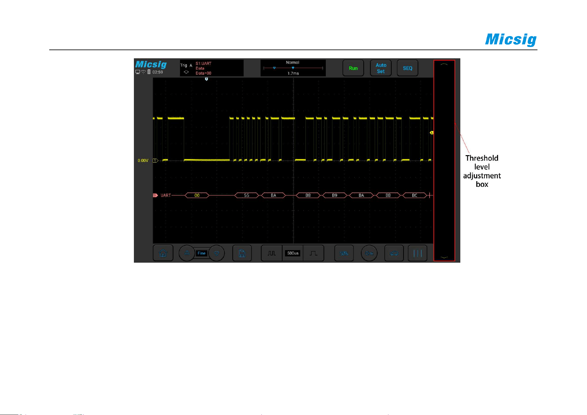
320
Figure 12-7 UART Decode Level Adjustment
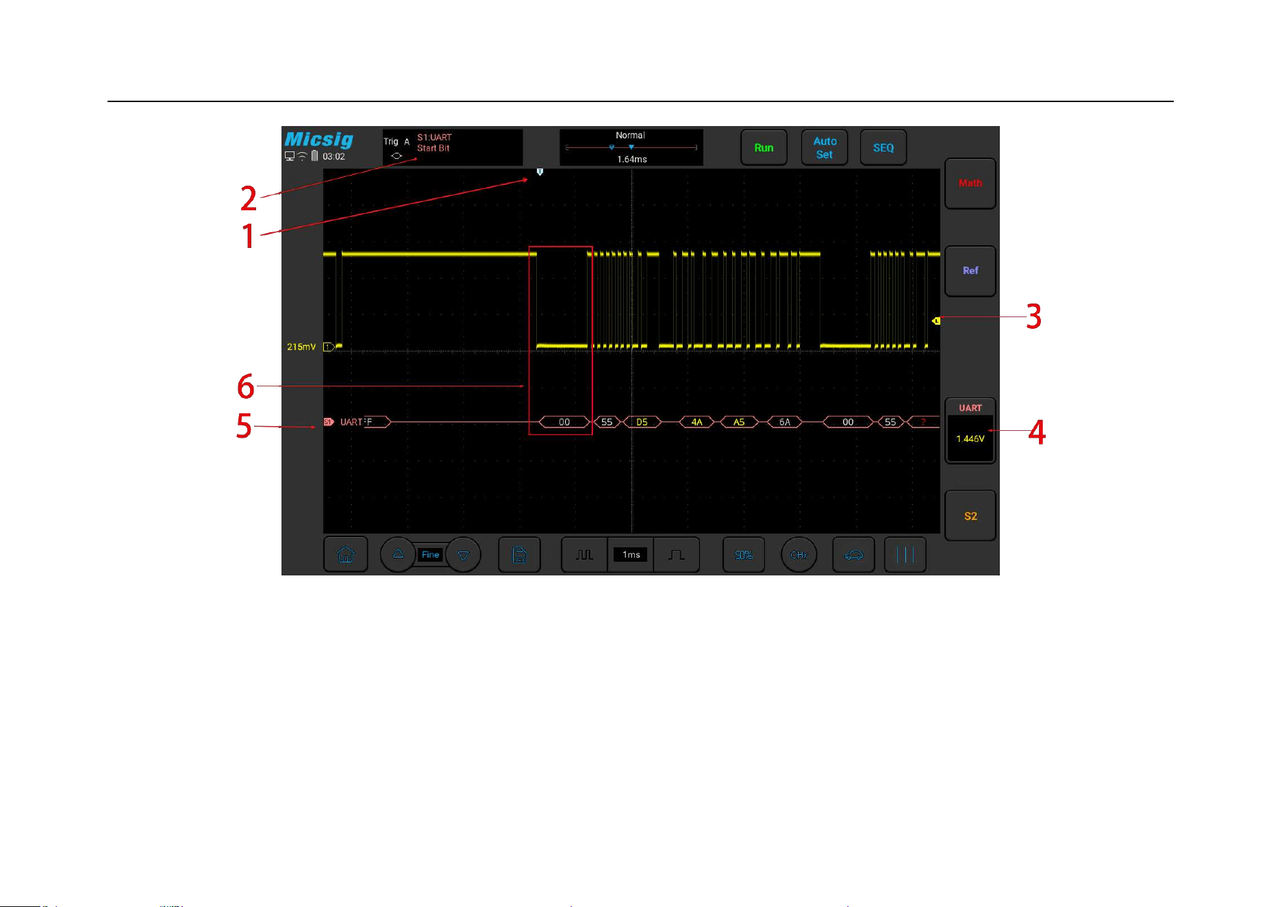
Chapter 12 Serial Bus Trigger and Decode (Optional)
321
Figure 12-8 UART Graphic Interface
UART graphic interface description:
(1) Trigger position
(2) Trigger type

322
(3) Threshold level
(4) Configuration information
(5) Decode the data packet, detailed as follows
(6) Decode data and the corresponding waveform area
UART decode data packet description:
(1) Decode data packet displays real-time data about the bus activities;
(2) Decode data displays as hexadecimal system in white;
(3) When the word length is 5-8 bits, the decode data displays as two bits of hexadecimal; when the word
length is 9 bits, the decode data displays as 3 bits of hexadecimal, and the 9th bit displays at the left side;
(4) When there is error in decode data, if the error is at stop bit, the data displays in yellow, if it is parity error,
data displays in red;
(5) When “?” appears, the time base needs to be adjusted to view decode results.
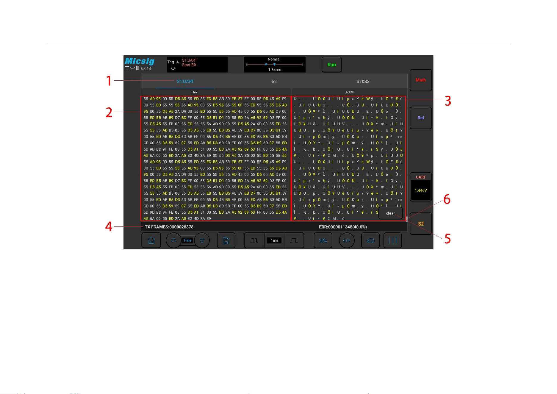
Chapter 12 Serial Bus Trigger and Decode (Optional)
323
Figure 12-9 UART Text Interface
UART text interface description, see Figure12-9:
(1) S1/S2/S1&S2 is channel configuration bus information.
(2) Area for decode data.

324
(3) ASCII code corresponding to the text data (when the data format is 9 bits and there is no parity bit, ASCII
code corresponds to lower 8 bits of data on the left side).
(4) Counter: Calculates the total number of frames and the percentage of ERR (parity error and stop bit error)
frames.
(5) Clear: Clear the counter data.
(6) Roller bar.
In the decode data area, the stop bit error data is displayed in yellow, and the decode error data is displayed in
red;
12.2 LIN Bus Trigger and Decode
For correctly decoding LIN bus data and making trigger stable, the bus configuration, trigger mode set and trigger
level need to be adjusted.
Bus configuration

Chapter 12 Serial Bus Trigger and Decode (Optional)
325
Left swipe or to open the bus configuration menu, and the following need to be set according to
measured signal:
Source — Select the signal source of decode.
Idle Level - high and low. Select whether to display high active or low active after the signal start bit of
measured equipment.
Baud Rate — Select the baud rate that matches the signal being measured, and it can be customized.
The setting method is the same as that of UART, and will not be repeated here. As shown in Figure 12-10:
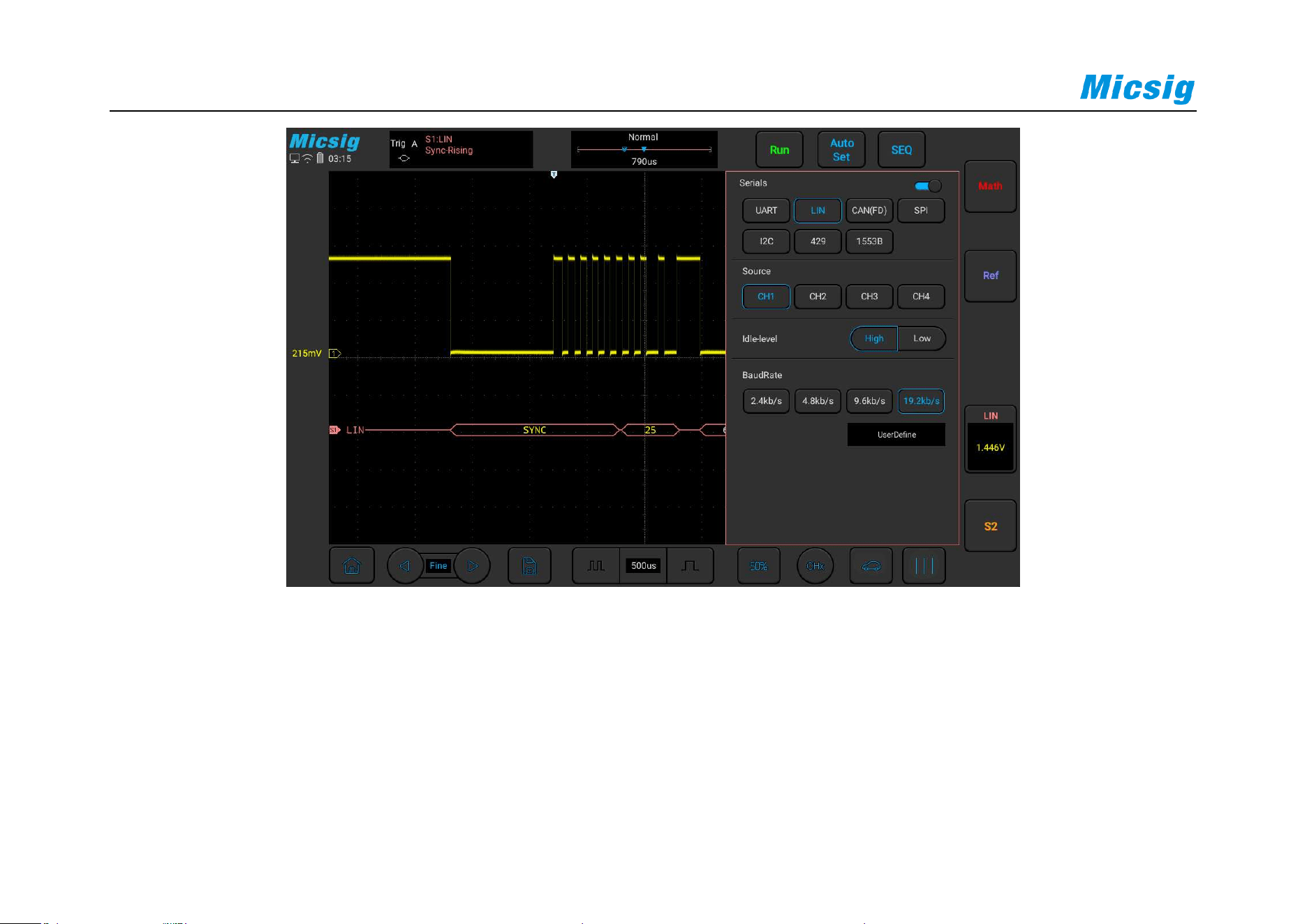
326
Figure 12-10 LIN Bus Configuration Menu
Trigger mode
Open the trigger configuration menu and select the appropriate trigger type. When the LIN bus trigger is
selected, the trigger mode includes: synchronous rising edge, frame ID, frame ID and data. See Figure 12-11:
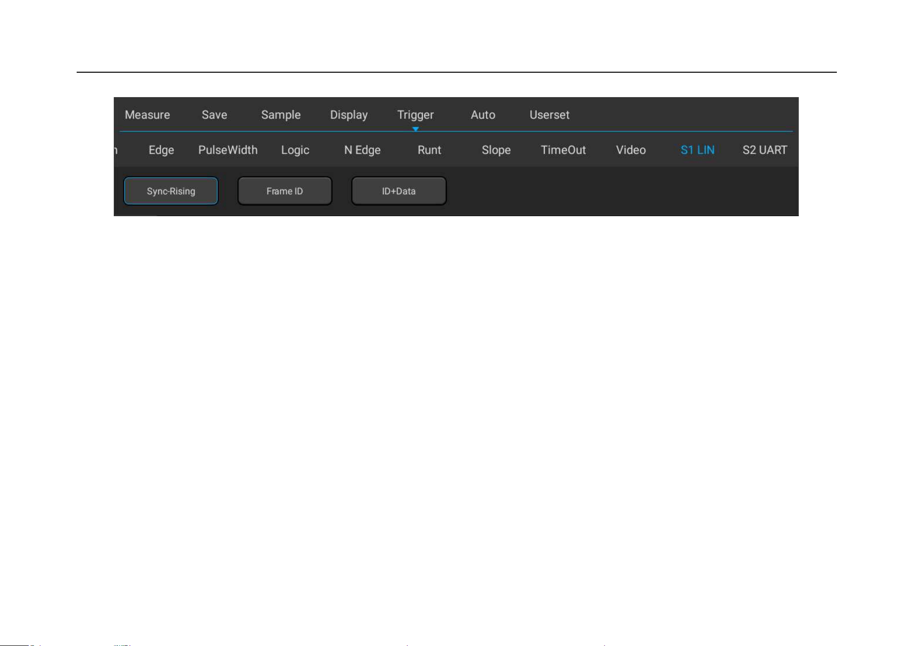
Chapter 12 Serial Bus Trigger and Decode (Optional)
327
Figure 12-11 LIN Trigger Mode Configuration Menu
a) Synchronous rising edge – When the “Sync Interval” of LIN bus ends, the rising edge triggers.
b) Frame ID — Triggered when a frame with an ID equal to the set value is detected. Select “Frame ID”, click
data on the touch screen, and use the pop-up virtual keyboard to modify it.
c) Frame ID and data—triggered when a frame with ID and data equal to the set value is detected. After
selecting “Frame ID and Data”, click ID or data, and set them.
LIN serial decode
Ch1 is connected to measured signal. The idle level is high and the baud rate is 19.2 kb/s. The trigger mode is
synchronous rising edge. Please follow these steps:

328
(1) Tap S1 to open the decode channel, and click again to open the bus configuration menu;
(2) Select the bus type as “LIN”, click “Ch1”, “Idle High”, “19.20kb/s”, and then close the menu;
(3) Open the trigger mode configuration menu and click “Synchronous Rising Edge”;
(4) Click configuration information to open the decode channel threshold level adjustment box, and drag
the adjustment box upward and downward to adjust the threshold level; adjust the threshold level according
to the signal amplitude level to make the signal stably triggered. The LIN trigger graphic interface is shown
in Figure 12-12:
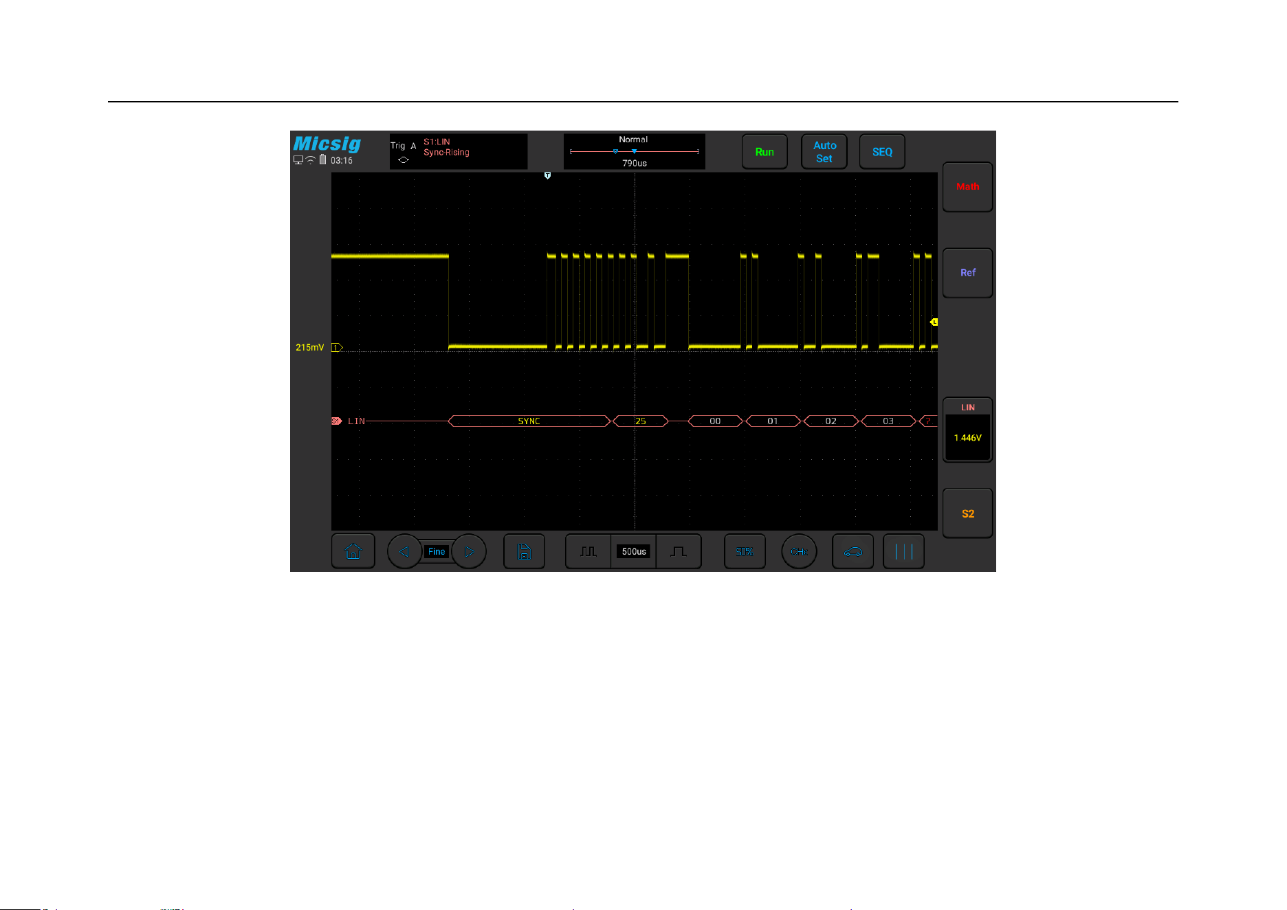
Chapter 12 Serial Bus Trigger and Decode (Optional)
329
Figure 12-12 LIN Graphic Interface
LIN decode data packet description:
(1) Decode data packet displays real-time data about the bus activities.
(2) Decode data displays as hexadecimal system.
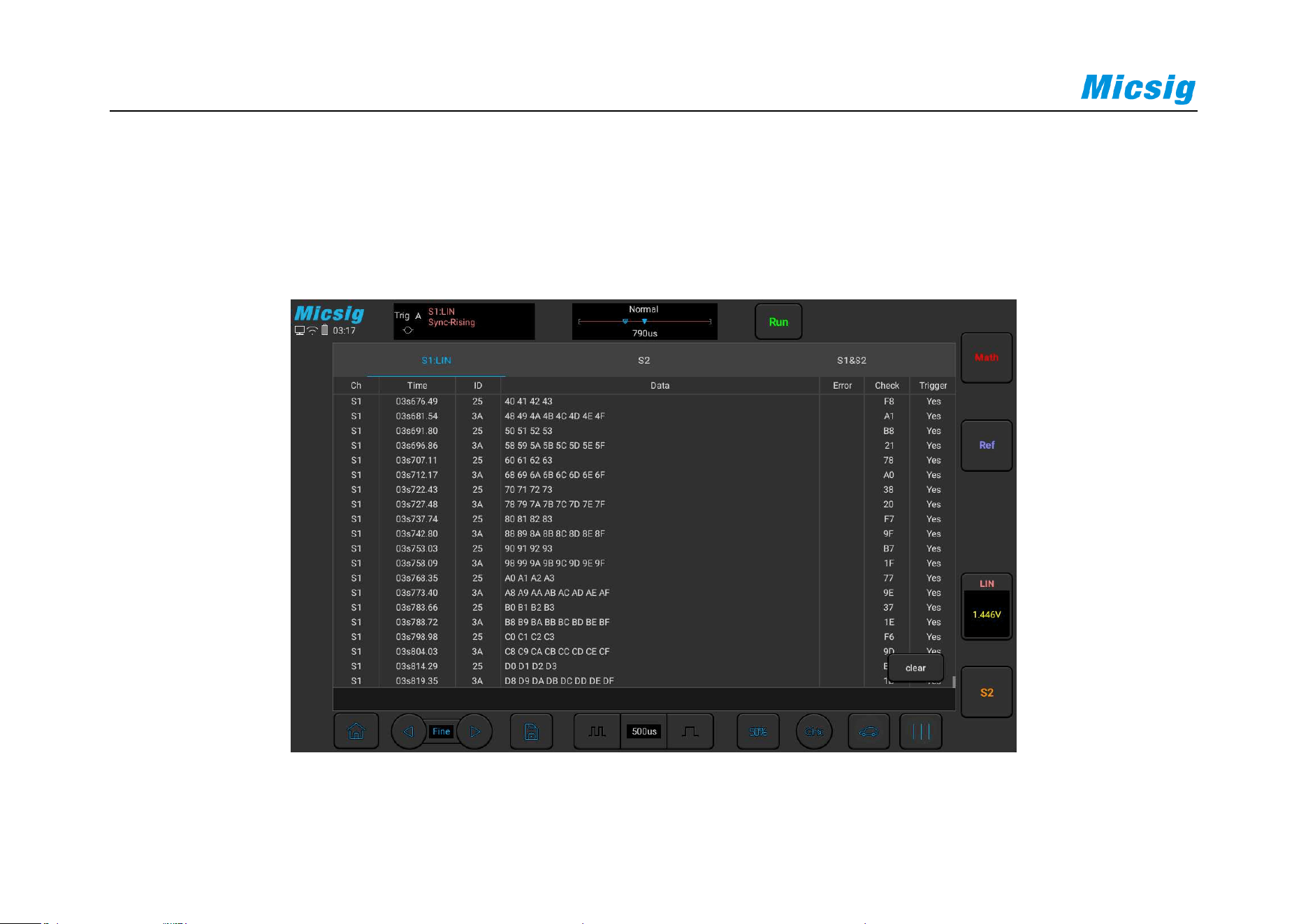
330
(3) “Frame ID” displays in yellow, “Data” displays in white, and “Parity sum” displays in green. If the parity
sum has error, it is displayed in red “E”.
(4) When “?” appears, the time base needs to be adjusted to view decode results.
Figure 12-13 LIN Text Interface

Chapter 12 Serial Bus Trigger and Decode (Optional)
331
LIN text interface description, as shown in Figure 12-13:
(1) “Ch”: bus channel.
(2) “Time”: Time intervals between the last frames to current frames.
(3) “ID”: Frame ID value.
(4) “Data”: Frame data.
(5) “Parity sum”: Frame parity sum, the sum of parity error displays in red.
(6) “Trigger”: “Yes” means the frame reaches trigger condition.
(7) “Clear”: Clear counter data.

332
12.3 CAN Bus Trigger and Decode
For correctly decoding CAN and CAN FD(optional) bus data and making trigger stable, the bus configuration,
trigger mode set and trigger level need to be adjusted.
Bus configuration
Left swipe or to open the bus configuration menu, the signal source needs to be set, and the signal
type and baud rate are set according to measured signal; the setting method is the same as that of UART and will
not be repeated here. See Figure 12-14:
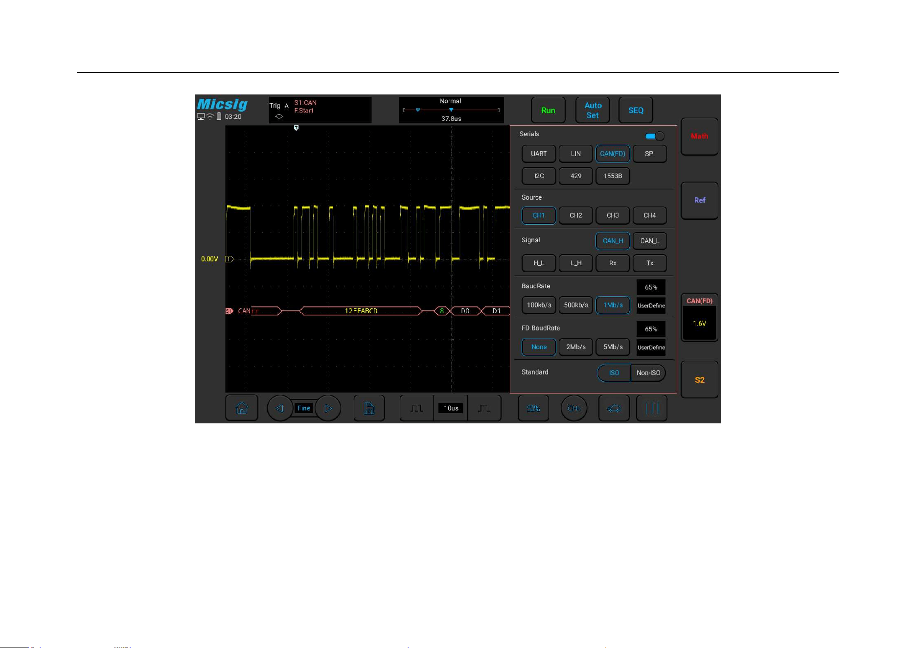
Chapter 12 Serial Bus Trigger and Decode (Optional)
333
Figure 12-14 CAN Bus Configuration Menu
Trigger mode
Open the trigger configuration menu and select the appropriate trigger type; when S1 CAN bus trigger is
selected, as shown in Figure 12-15:
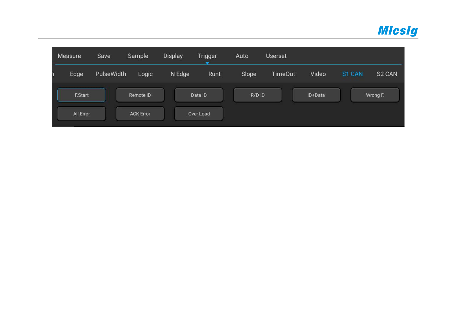
334
Figure 12-15 CAN Trigger Mode Configuration Menu
Trigger mode selection menu description:
a) Frame start — trigger at the start of the frame;
b) Remote frame ID — setting the ID matches the remote frame trigger. After selecting the “Remote Frame
ID”, and then set the ID value at the bottom of the trigger data area
Operation description: Press the numbers on the touch screen and use the virtual keyboard to set;
c) Data framed ID — trigger on data frame that matches set ID. Data frame ID configuration mode is the
same as the remote data frame ID configuration;

Chapter 12 Serial Bus Trigger and Decode (Optional)
335
d) Remote frame/data frame ID — trigger on remote frame or data frame that matches set ID. Remote
frame/data frame ID configuration is the same as the remote data frame ID configuration;
e) Data frame ID and data ID — trigger on data frame that matches set ID and data. The configuration method
is the same as the remote frame ID configuration;
f) Error frame — trigger on CAN error frame;
g) All errors — trigger when there is any error in format or activity;
h) Ack error — trigger on recessive (high) Ack position;
i) Overload frame — trigger on CAN overload frame.
CAN serial decode
Ch1 is connected to measured signal. The idle level is high and the baud rate is 1Mb/s; the Trigger mode is the
frame start. Please follow these steps:
(1) Tap S1 to open the decode channel, and click S1 again to open the bus configuration menu;
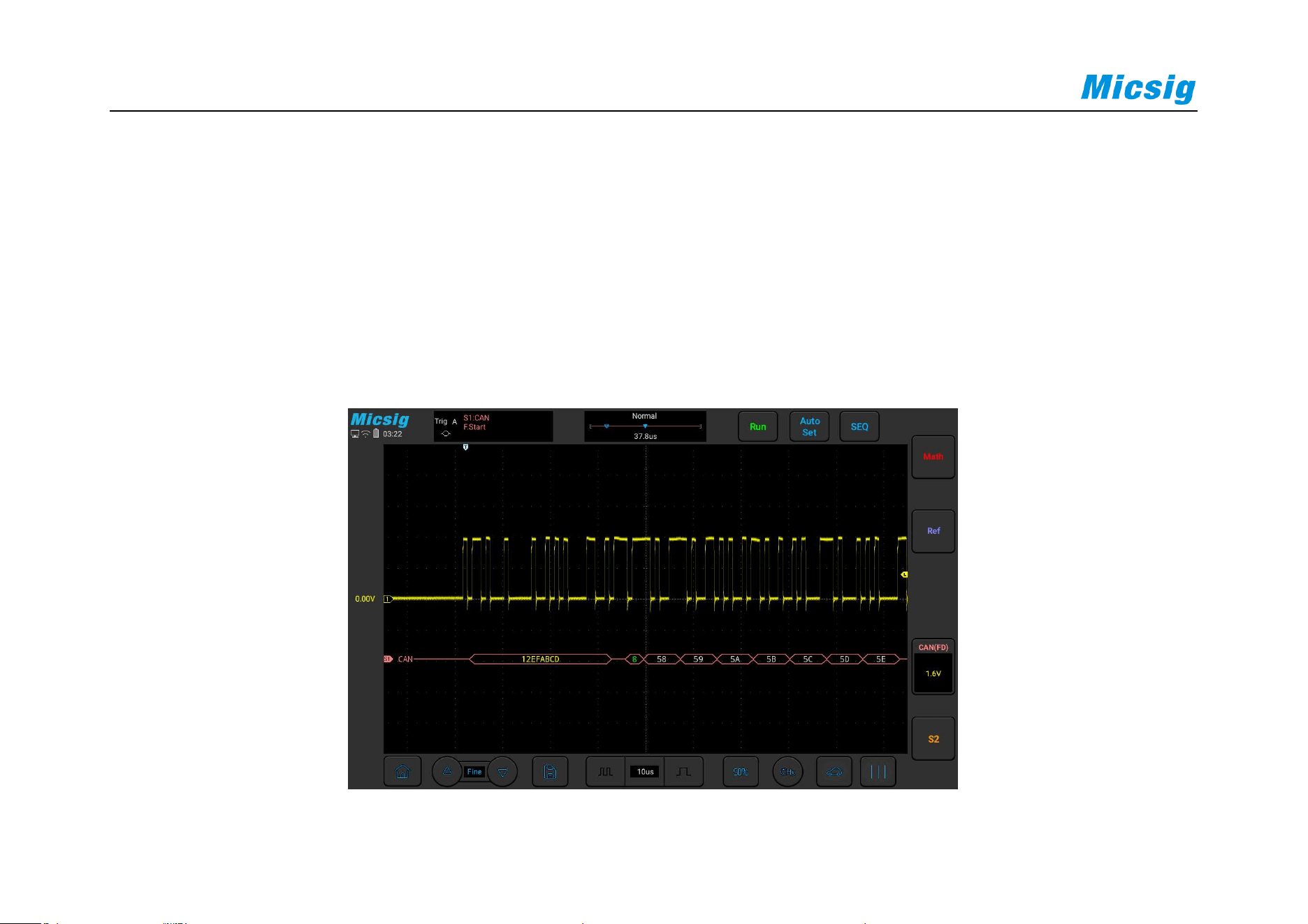
336
(2) Select the bus type as “CAN”, and then click “Ch1”, “Idle High” and “1Mb/s”. After setting, click the
blank area to close the menu;
(3) Open the trigger mode configuration menu and click “Frame Start”;
(4) Adjust the threshold level according to the signal amplitude; the CAN trigger graphic interface is shown in
Figure 12-16:
Figure 12-16 CAN Graphic Interface

Chapter 12 Serial Bus Trigger and Decode (Optional)
337
CAN decode data packet description:
(1) Decode data packet displays real-time data about the bus activities.
(2) Decode data displays as hexadecimal system.
(3) “Frame ID” displays in yellow, “Data” displays in white, and “DLC” and “CRC” codes display in green. If
there is frame error, it is displayed in red “E”.
(4) When “?” appears, the time base needs to be adjusted to view decode results, and “!” indicates that the bus
waveform corresponding to the decode data packet is incomplete and the data cannot be displayed
correctly.
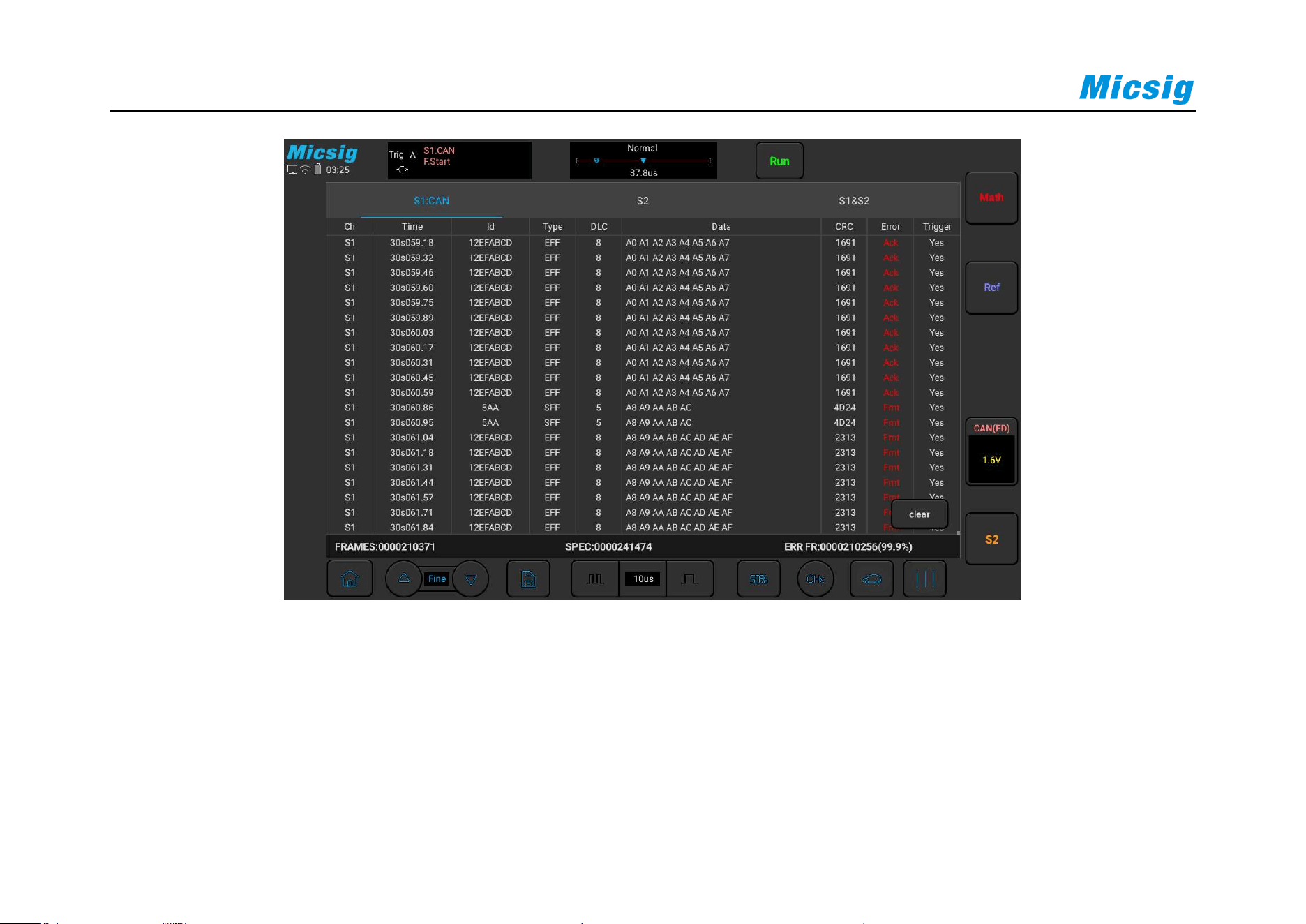
338
Figure 12-17 CAN Text Interface
CAN text interface description, as shown in Figure 12-17:
(1) “Ch”: bus channel.
(2) “Time”: Time intervals between the last frames to current frames.

Chapter 12 Serial Bus Trigger and Decode (Optional)
339
(3) “ID”: CAN frame ID value displayed in hexadecimal, maximum 29 bits.
(4) “Type”: Frame type, “SFF” standard data frame, “SRF” standard remote frame, “EFF” extended data
frame, “ERF” extended remote frame.
(5) “DLC”: Number of data bytes sent by this frame. This value can be ignored for remote frames.
(6) “Data”: Frame data.
(7) “CRC”: Frame CRC check code.
(8) “Error”: Response error, bit stuffing error, format error, CRC error.
(9) “Trigger”: “Yes” means the frame reaches trigger condition.
(10) “Statistics”: counts the number of occurrences of frame type, data length, status, etc., and the percentage.
12.4 SPI Bus Trigger and Decode
For correctly decoding SPI bus data and making trigger stable, the bus configuration, trigger mode set and trigger
level need to be adjusted.
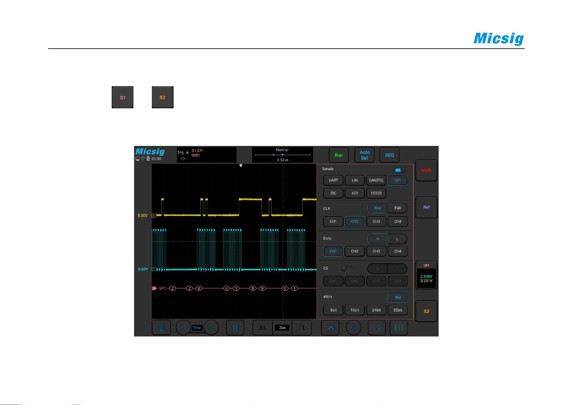
340
Bus configuration
Left swipe or to open the bus configuration menu, the following need to be set:
Clock source, data source, chip select signal, and data word length, as shown in Figure 12-18:
Figure 12-18 SPI Bus Configuration Menu
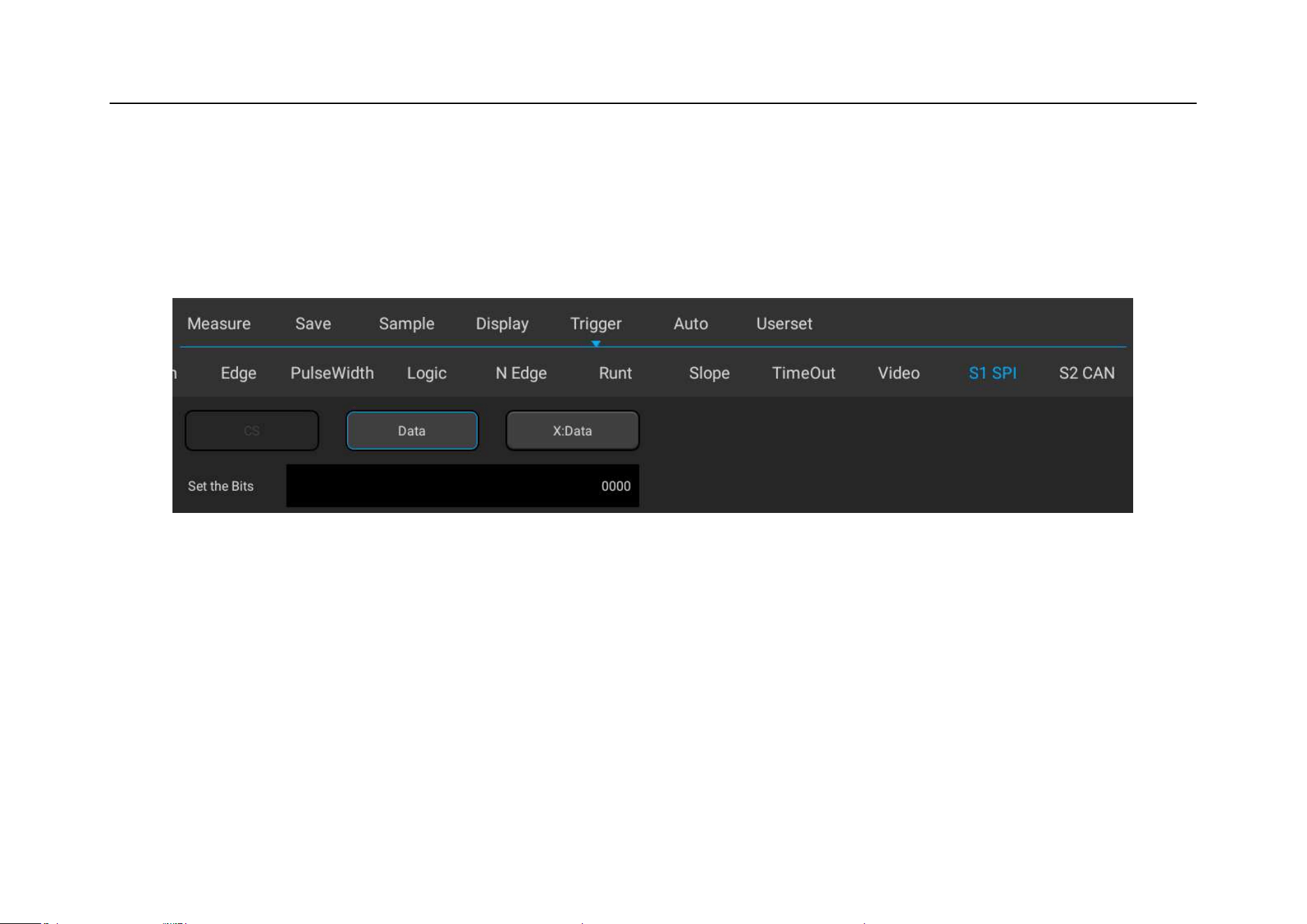
Chapter 12 Serial Bus Trigger and Decode (Optional)
341
Trigger mode
Open the trigger configuration menu and select the appropriate trigger type; when selecting the SPI bus trigger,
as shown in Figure 12-19:
Figure 12-19 SPI Trigger Mode Configuration Menu
The operation method is the same as CAN frame ID to be matched in the configuration, and will not be repeated
here.
Note: According to the data byte length set by bus decode, the value of the relevant bit within the byte length is
set. Trigger when the corresponding bit on data bus matches the set value.

342
SPI serial bus
The measured signal channel Ch1 is connected to CLK, Ch2 channel is connected to DATA, the bus idle state is
high, the clock rising edge is sampled; the data word length is 4 bits; the CS chip select is off; the trigger mode
matches the “Data” at 0001, please follow the steps below:
(1) Tap S1 to open the decode channel, and click S1 again to open the bus configuration menu;
(2) Select the bus type as “SPI”, click clock as “Ch1” rising edge, the data is “Ch2” high level, and the data
word length is “4bit”;
(3) Open the trigger setting menu, click data on the touch screen, and use the virtual soft keyboard to set the
data to be matched as “0001”;
(4) Adjust the threshold levels of two channels according to signal amplitude; the SPI trigger graphic interface
is shown in Figure 12-20:
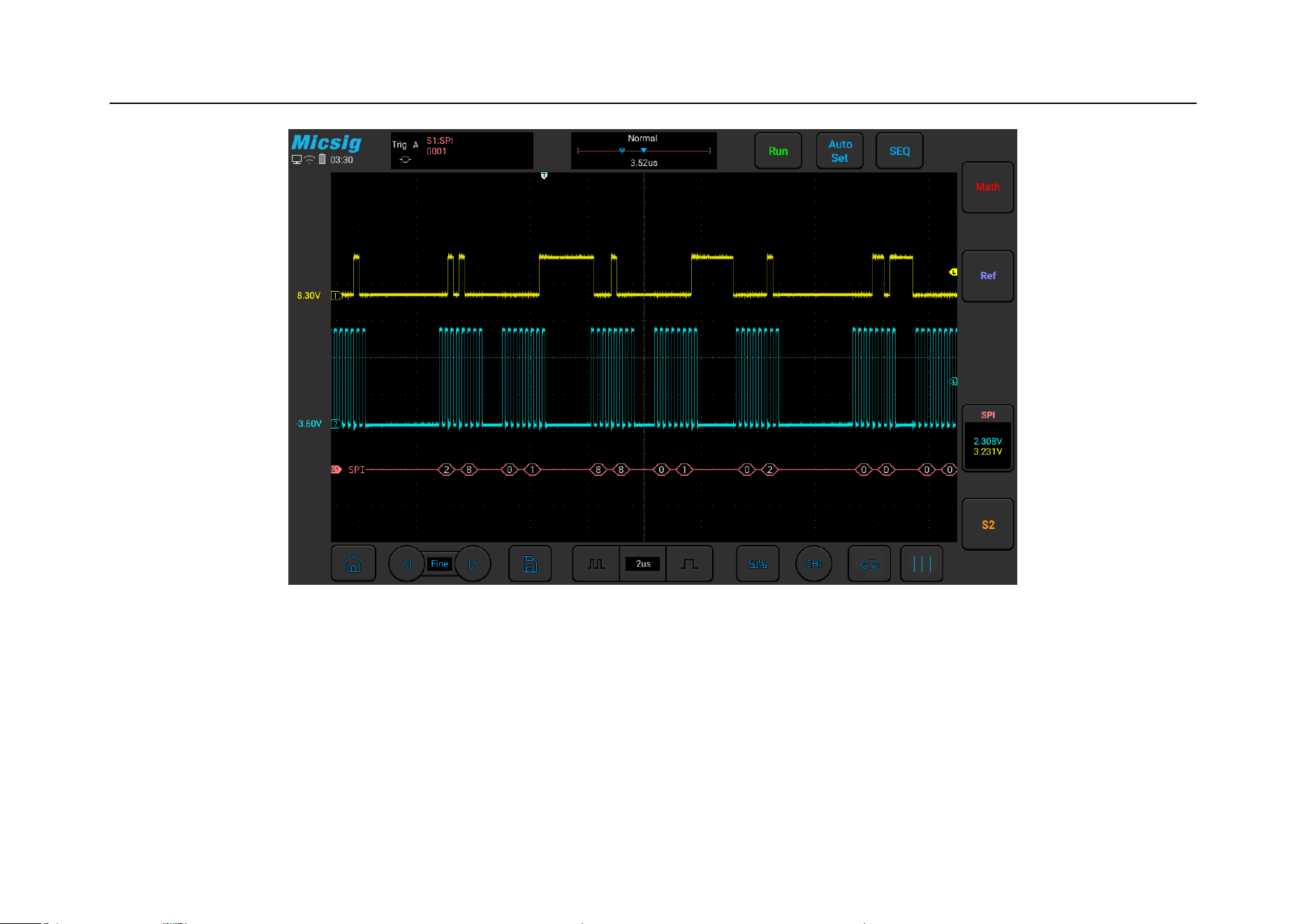
Chapter 12 Serial Bus Trigger and Decode (Optional)
343
Figure 12-20 SPI Graphic Interface
SPI decode data packet description:
(1) Decode data packet displays real-time data about the bus activities.
(2) Decode data displays as hexadecimal system.
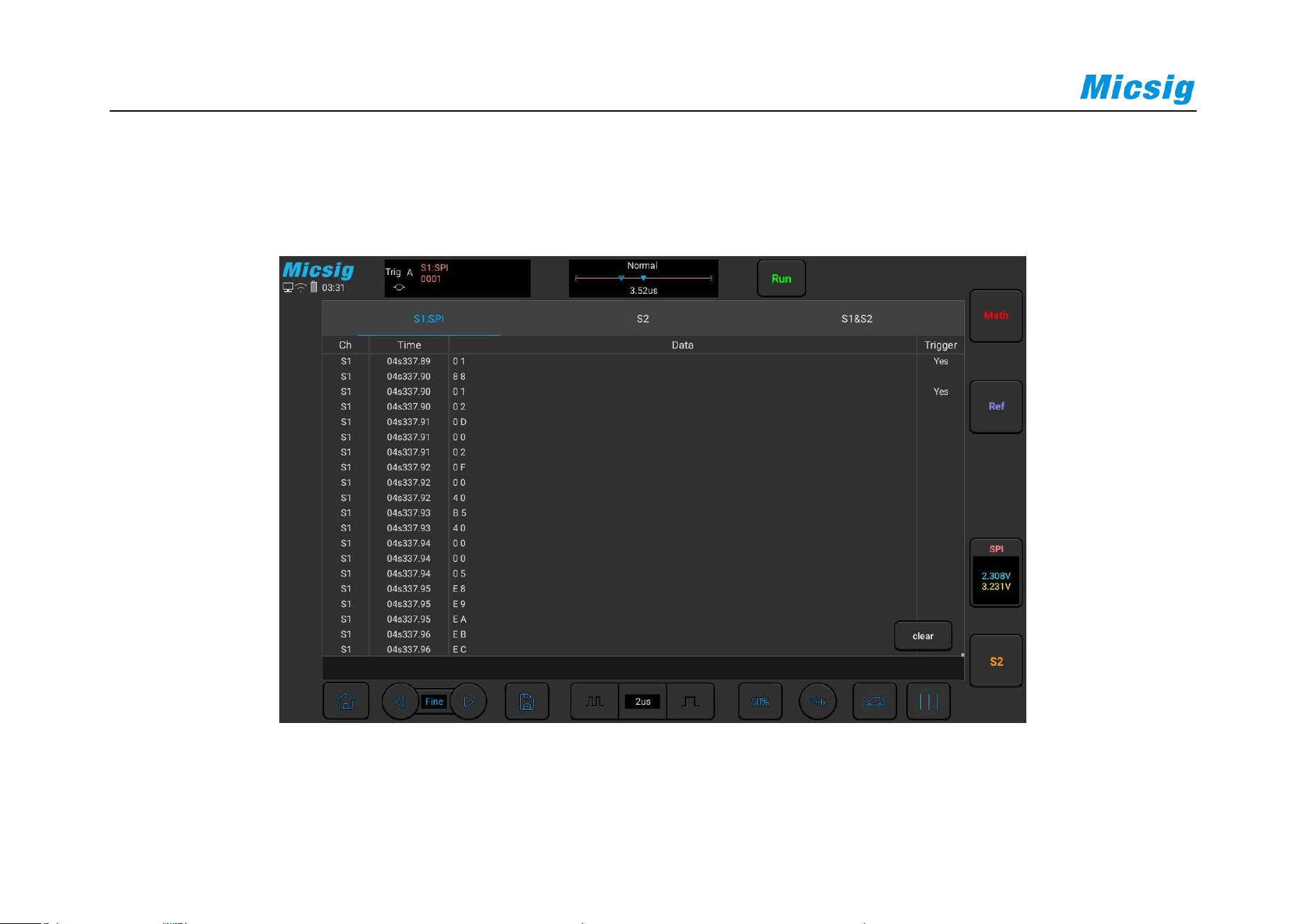
344
(3) Data displays in white.
(4) When “?” appears, the time base needs to be adjusted to view decode results.
Figure 12-21 SPI Text Interface

Chapter 12 Serial Bus Trigger and Decode (Optional)
345
SPI text interface description, as shown in Figure 12-21:
(1) “Ch”: bus channel.
(2) “Time”: Time intervals between the last frames to current frames.
(3) “Data”: According to the data word length setting, the decode data is displayed. For example, if the data
word length is 8bit, only one byte displays in the data column; if the data word length is 16bit, 2 bytes
display in the data column; if the data word length is 24bit, 3 bytes display; and if the data word length is
32bit, 4 bytes display.
(4) “Trigger”: “Yes” means the frame reaches trigger condition.
Note: “One frame” is measured by the set “data word length” and can meet 1 data bit code stream.

346
12.5 I2C Bus Trigger and Decode
For correctly decoding I2C bus data and making trigger stable, the bus configuration, trigger mode set and trigger
level need to be adjusted.
Bus configuration
Left swipe or to open the bus configuration menu, Bus configuration includes the serial clock
(SCL) and the serial data (SDA) corresponding to the channel settings. See Figure 12-22:
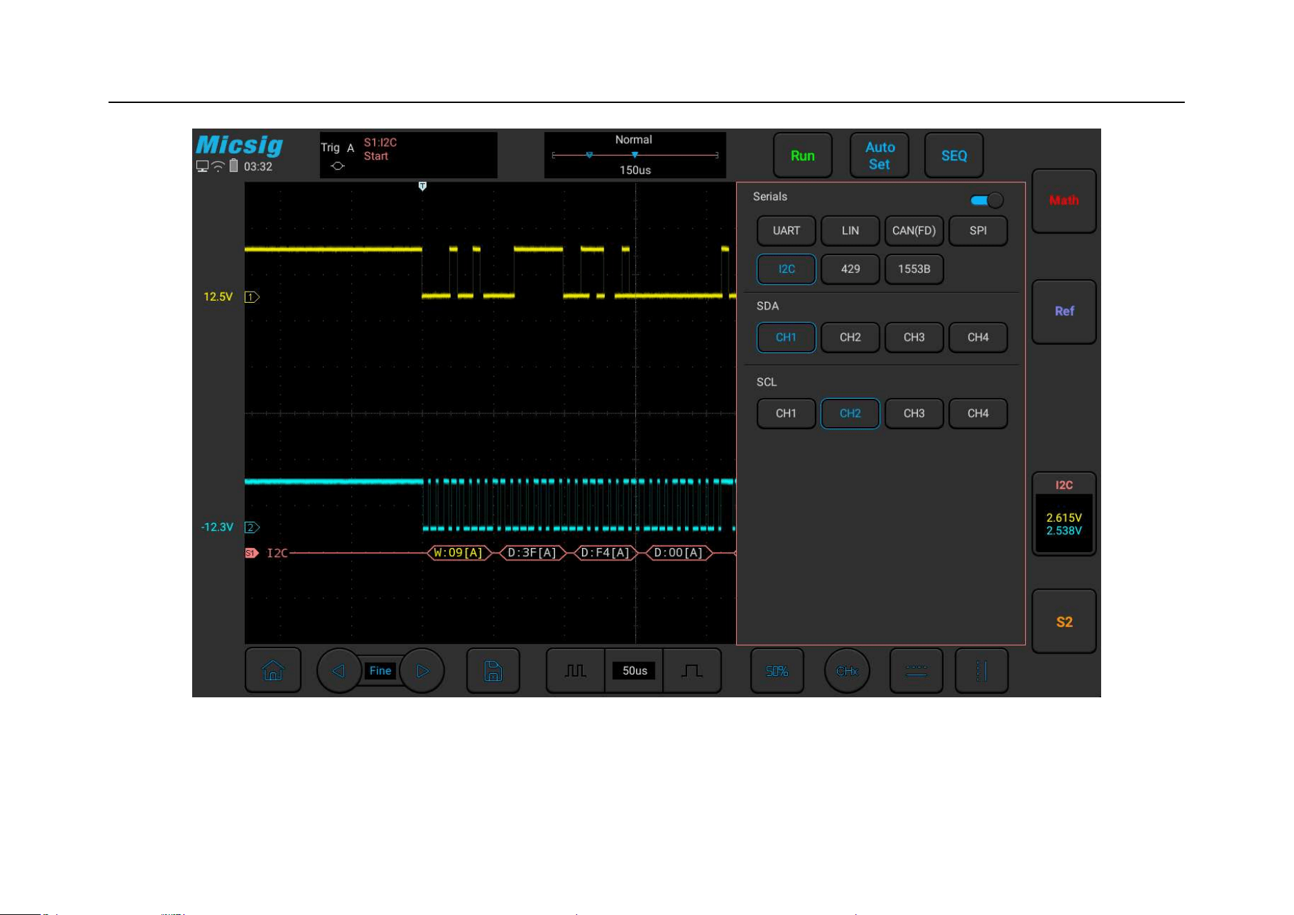
Chapter 12 Serial Bus Trigger and Decode (Optional)
347
Figure 12-22 I2C Bus Configuration Menu
Notes: When SCL or SDA channel is set, the system will automatically set other channels.
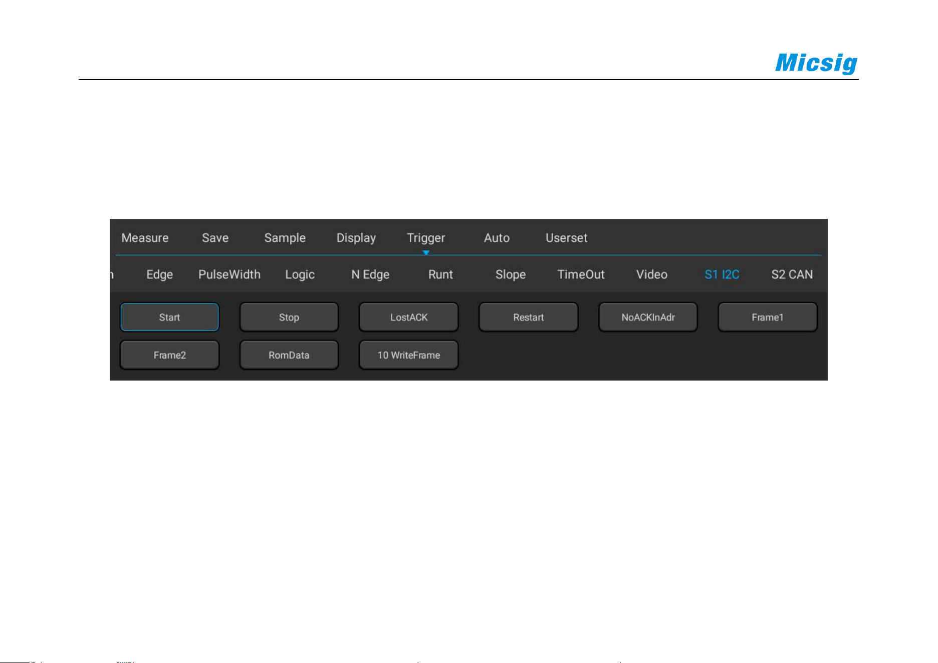
348
Trigger mode
Open the trigger configuration menu and select the appropriate trigger type. When the I2C bus trigger is
selected, click the trigger type and relationship on the screen, as shown in Figure 12-23:
Figure 12-23 I2C Trigger Mode Configuration Menu
Trigger mode menu description:
a) Start condition — trigger when SCL is high and SDA has a falling edge (includes restart).
b) Stop condition — trigger when SCL is high and SDA has a rising edge.
c) Ack Loss — Trigger when the bus Ack bit is high.

Chapter 12 Serial Bus Trigger and Decode (Optional)
349
d) Restart — triggered when a new start condition occurs before the stop condition.
e) Address no ack — trigger when the ack bit in the set address field is invalid (ignoring W/R bit), select
“Address” in the trigger data, and use the pop-up virtual soft keyboard to modify it.
f) Frame Type 1 - Start + Address 7 + Read/Write + Acknowledge + Data; if all bits in the frame type match,
trigger on read/write frames in 7-bit addressing mode on the 17th clock edge.
Frame type 1 operation method: Select values after the address/data, click values after the address/data on
the touch screen, and modify them on the pop-up virtual soft keyboard.
g) Frame type 2 — Start + Address 7 + Read/Write + Acknowledge + Data 1 + Acknowledge + Data 2; trigger
on read/write frames in 7-bit addressing mode on the 26th clock edge if all bits in the frame type match.
The operation method of configuring frame type 2 is the same as frame type 1, and will not be repeated
here.
h) EEPROM data read - When the read operation which contains 1010xxx control byte of the EEPROM
appears on the bus and the Ack bit is correct, then the read data can be captured. If the captured data and

350
the set data match the set relationship condition, trigger on the clock edge of Ack bit after the data byte.
After selecting “EEPROM Data Read”, click the relationship by “=” “ >” “<” “ ≠”, and the setting method
is the same as the address field.
i) 10-bit write frame - Trigger on 10-bit write frame on the 26th clock edge if all bits in the pattern match.
Trigger mode is start condition, SCL connect to Ch2, SDA connect to Ch1, follow these steps as below:
(1) Tap S1 to open the decode channel, and click S1 again to open the bus configuration menu;
(2) Select the bus type as “I2C”, open the bus setting menu, and select the clock SCL as Ch2 channel;
(3) Open the trigger mode configuration menu and click “Start Condition” on the touch screen.
(4) Set the threshold level of two channels according to signal amplitude; I2C trigger graphic interface is
shown in Figure 12-24:
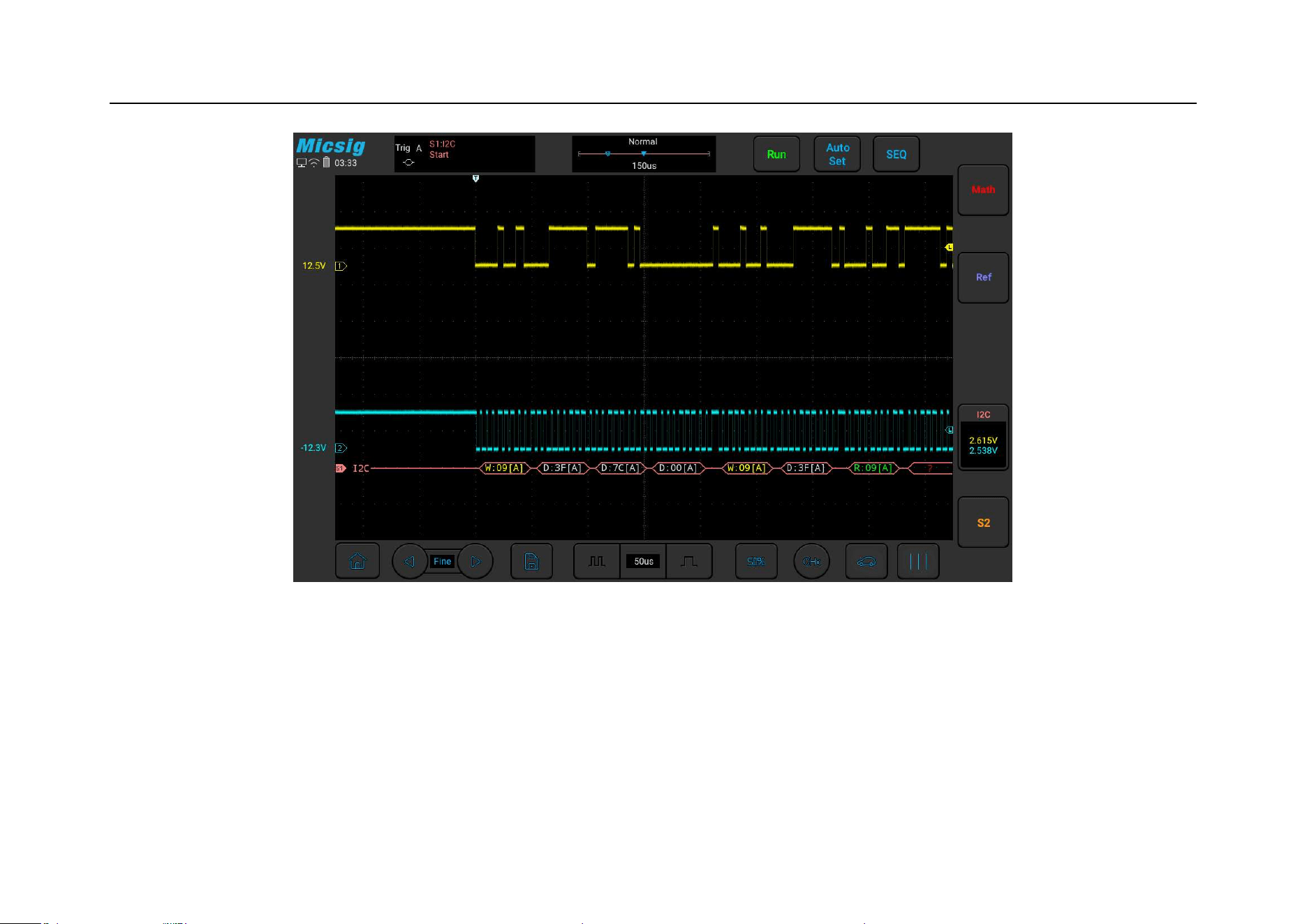
Chapter 12 Serial Bus Trigger and Decode (Optional)
351
Figure 12-24 I2C Graphic Interface
I2C decode data packet description:
(1) Decode data packet displays real-time data about the bus activities.
(2) Decode data displays as hexadecimal system.
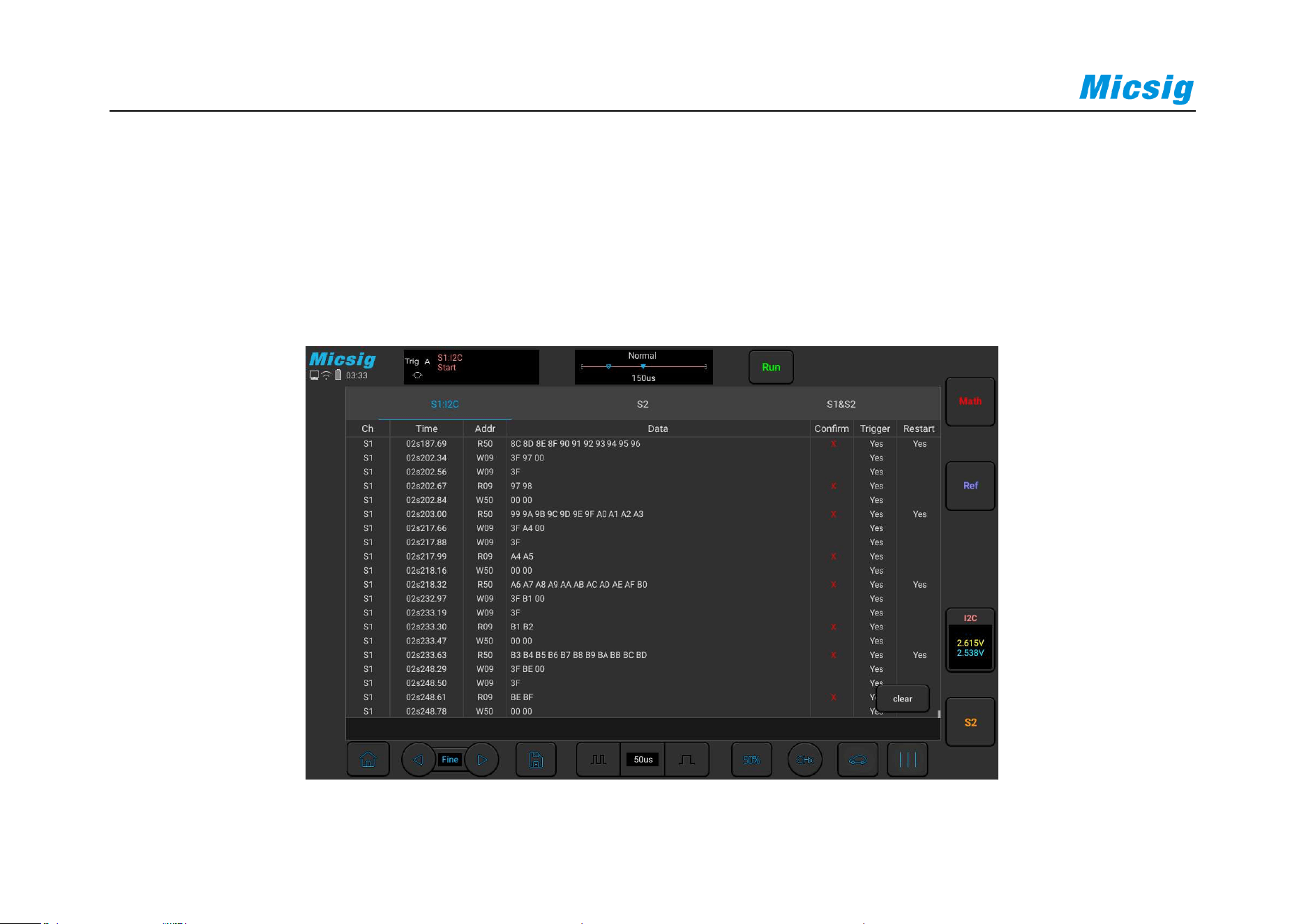
352
(3) Address content display: Read address displays in green, write address displays in yellow, and data displays
in white. “W” denotes write operation, “R” denotes read operation, “D” denotes decode data, and “~A”
denotes no Ack bit.
(4) When “?” appears, the time base needs to be adjusted to view decode results.
Figure 12-25 I2C Text Interface

Chapter 12 Serial Bus Trigger and Decode (Optional)
353
I2C text interface description, as shown in Figure 12-25:
(1) “Ch”: bus channel.
(2) “Time”: intervals between the last read/write operations to current read/write operations
(3) “Address”: in address bar, “R” means the read operation, and “W” means write operation
(4) “Data”: data sent by one read and write operation is in the data bar.
(5) “Ack”: in Ack bar, “X” means Ack bit lost.
(6) “Trigger”: “Yes” means reach trigger condition.
(7) “Restart”: “Yes” means reach restart condition.

354
12.6 ARINC429 Bus Trigger and Decode
For correctly decoding ARINC429 bus data and making trigger stable, the bus configuration, trigger mode set and
trigger level need to be adjusted.
Bus configuration
Left swipe or to open the bus configuration menu, the following needs to be set:
Data Source — Select channel for ARINC 429 signal.
Word format — Select ARINC 429 decode mode.
Bus Display — Set the format for ARINC 429 decode data.
Baud Rate — Set the speed of ARINC 429 signal.
As shown in Figure 12-26:
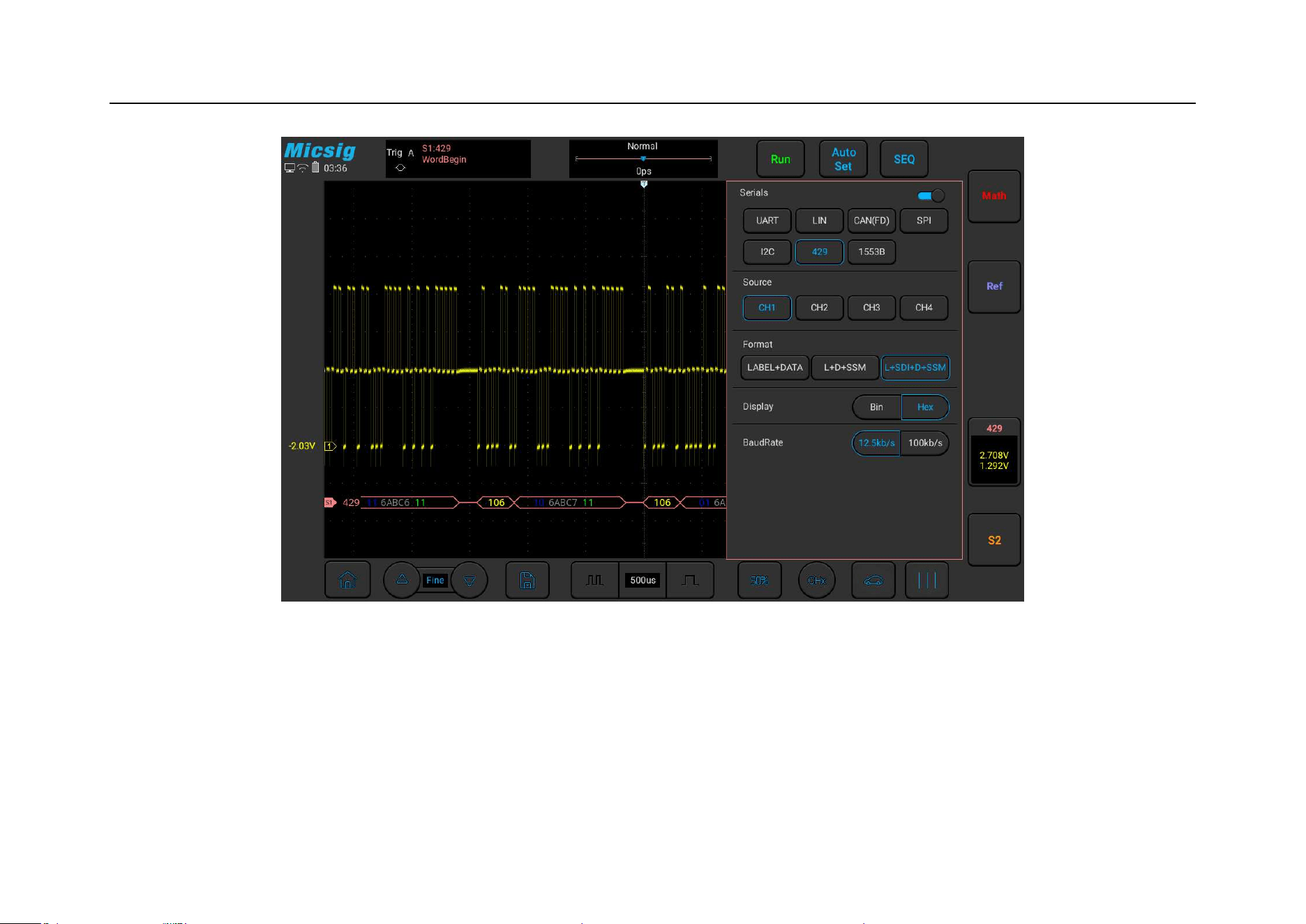
Chapter 12 Serial Bus Trigger and Decode (Optional)
355
Figure 12-26 ARINC429 Bus Configuration Menu
Trigger mode
Open the trigger configuration menu and select the appropriate trigger type; when the ARINC429 bus trigger is
selected, click the trigger type and relationship on the screen, as shown in Figure 12-27:
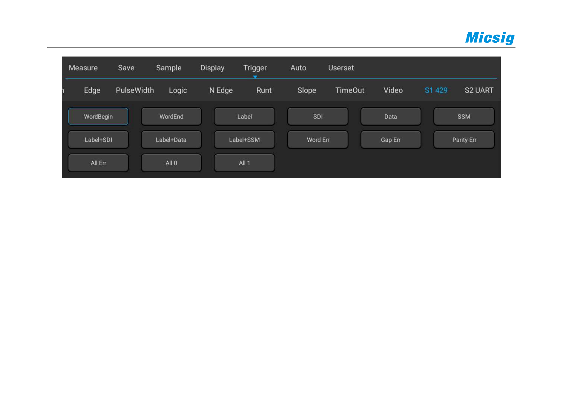
356
Figure 12-27 ARINC429 Trigger Mode Configuration Menu
If LABEL, SDI (source identifier), DATA or SSM (symbol/status mark) trigger are used, after selecting trigger
mode, use the pop-up virtual keyboard to modify it, enter the value, and click “Enter” on the virtual soft
keyboard to complete the setting.
Trigger configuration menu description:
a) Word start: Trigger at the word start.
b) Word stop: Trigger at the word stop.

Chapter 12 Serial Bus Trigger and Decode (Optional)
357
c) LABEL: Label, triggered when the specified tag value occurs.
d) SDI: Source identifier, triggered on the specified source terminal.
e) DATA: Trigger on the specified data.
f) SSM: Symbol/status mark, triggered on the specified symbol status matrix.
g) LABEL+SDI: Trigger on the specified label and the specified source terminal.
h) LABEL+DATA: Trigger on the specified label and the specified data.
i) LABEL+SSM: Trigger on the specified label and the specified symbol status matrix.
j) Word Error - Triggered when a word error occurs.
k) Word gap error: Triggered when a gap error occurs.
l) Verification error: Triggered when a verification error occurs.
m) All errors: Triggered when any of the above errors occur.
n) All 0 bits: Triggered when any bit with the value of zero occurs.

358
o) All 1 bit -: Triggered when any bit with the value of 1 appears.
ARINC 429 serial decode
The measured signal source is CH1, the decode format is LABEL+DATA, the display is in hexadecimal, the
baud rate is 12.5kb/s, and the trigger mode is LABEL, operate as follows:
(1) Tap S1 to open the decode channel, and click S1 again to open the bus configuration menu;
Select bus type “429”, source as “CH1”, decode format as “LABEL+DATA”, display in “hexadecimal”,
baud rate as 12.5kb/s.
(2) Open the trigger setting menu, select the trigger type as bus trigger, S1-ARINC429, the trigger mode is
LABEL, and enter LABEL as “106” on virtual keyboard.
Adjust High trigger threshold level and Low trigger threshold level according to signal amplitude; and
ARINC429 trigger graphic interface is shown in Figure 12-28:
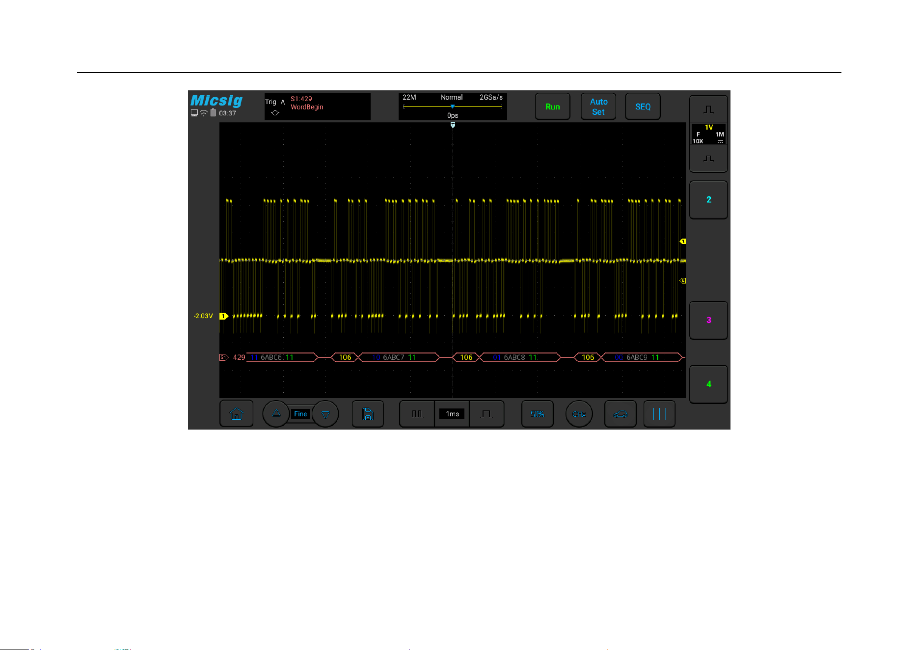
Chapter 12 Serial Bus Trigger and Decode (Optional)
359
Figure 12-28 ARINC429 Graphic Interface
ARINC429 decode data packet description:
(1) Data packet, a total of 32bits, the data format is 8~1 (label bit, high bit first) +9~10(SD) +11~29 (data bit,
low bit first) +30~31 (symbol status bit) +32 (parity bit)
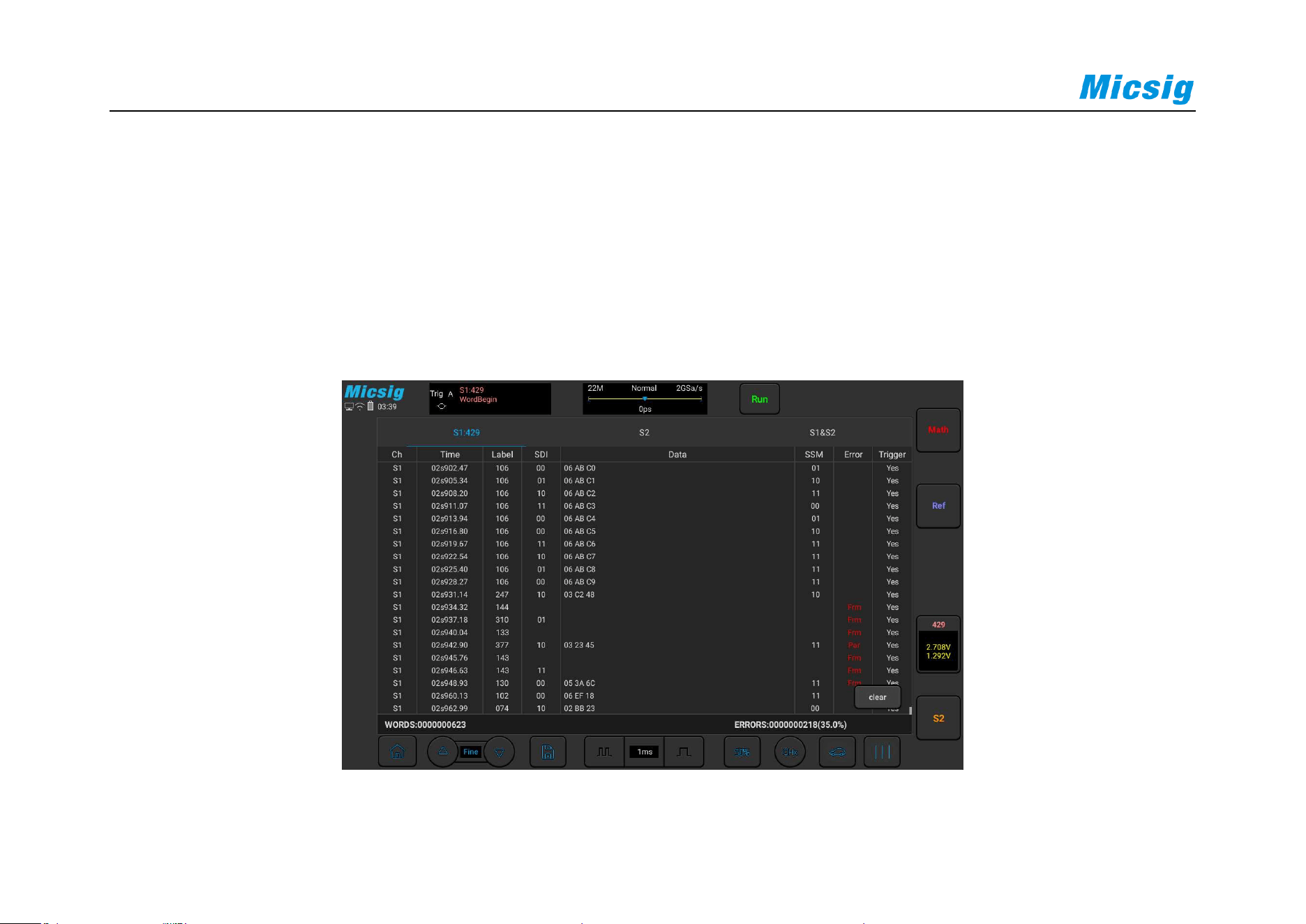
360
(2) Label (8bits) - Displayed in octal: yellow
(3) SDI (2bits) - Displayed in binary: blue
(4) Data (19bits) - Displayed in selected numeration system: white, or red if there is parity error
(5) SSM (2bits) - Displayed in binary: green
Figure 12-29 ARINC429 Text Interface

Chapter 12 Serial Bus Trigger and Decode (Optional)
361
ARINC429 text interface description, as shown in Figure 12-29:
(1) “Ch”: bus channel.
(2) “Time”: intervals between the last read/write operations to current read/write operations
(3) “LABLE”: label, information identifier, displayed in octal.
(4) “SDI”: source/target identifier, displayed in binary (displays XX if not identified separately).
(5) “Data”: content of the transmitted information, displayed in the selected numeration system.
(6) “SSM”: symbol/status matrix, displayed in binary (displays XX if not identified separately).
(7) “Error”: displays the frame error type (parity error Par, frame error Frm).
(8) “Trigger”: “Yes” means reach trigger condition.

362
12.7 1553B Bus Trigger and Decode
For correctly decoding 1553B bus data and making trigger stable, the bus configuration, trigger mode set and
trigger level need to be adjusted.
Bus configuration
Left swipe or to open the bus configuration menu, the data source and display hexadecimal need
to be set, as shown in Figure 12-30:
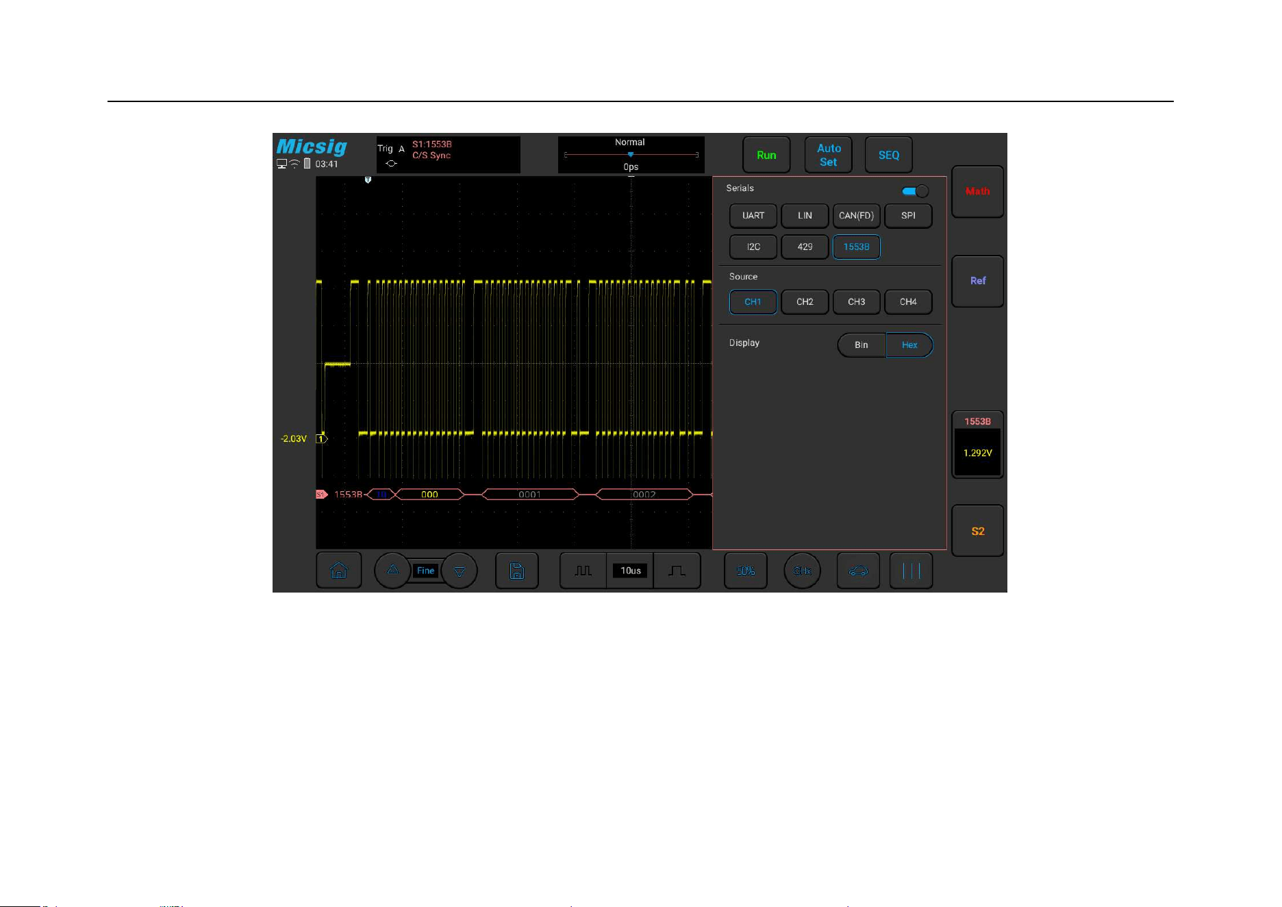
Chapter 12 Serial Bus Trigger and Decode (Optional)
363
Figure 12-30 1553B Bus Configuration Menu
Trigger mode
Open the trigger configuration menu and select the appropriate trigger type. When the trigger type is 1553B bus
trigger, click the trigger type on the screen, as shown in Figure 12-31:
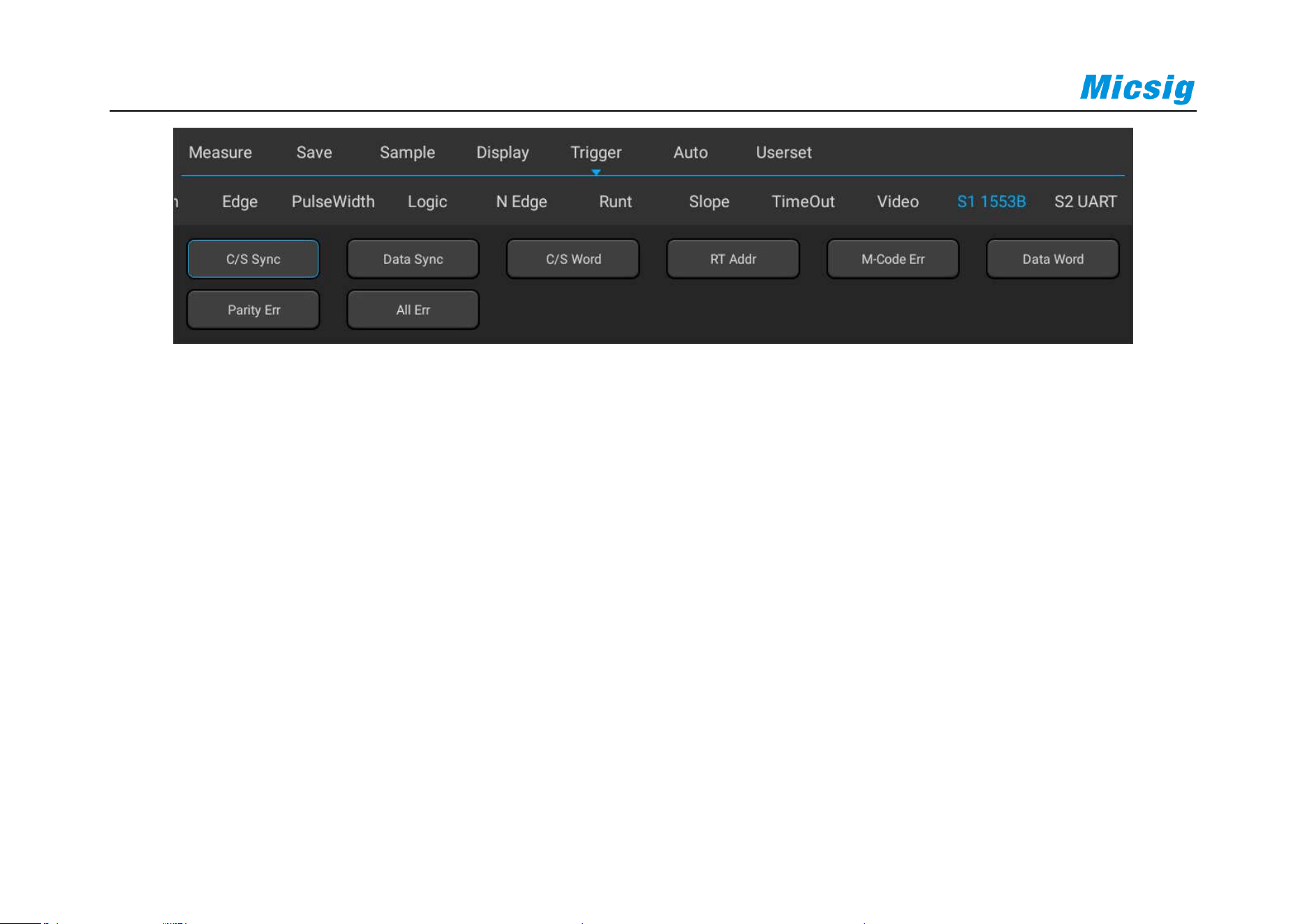
364
Figure 12-31 1553B Trigger Mode Configuration Menu
Trigger configuration menu description:
a) Command/status word sync header: Triggered at the beginning of the command/status word (at the end of
valid C/S sync pulse).
b) Data word sync header: Triggered at the beginning of data word (at the end of valid data sync pulse).
c) Command/status word: Triggered when the specified command/status word is detected.
d) Remote terminal address: Triggered when RTA of command/status word matches the specified value.

Chapter 12 Serial Bus Trigger and Decode (Optional)
365
e) If you select this option, RTA softkey will be available, allowing you to select the hexadecimal remote
terminal address value to be triggered on it. If you select 0xXX (irrelevant), oscilloscope will trigger on any
RTA.
f) Manchester coding error: Triggered when a Manchester coding error is detected.
g) Data word: Triggered when the specified data word is detected.
h) Odd parity error: Triggered when the odd parity bit is incorrect for data in the word.
i) All errors: Triggered when an error is detected.
1553B serial decode
The measured signal source is CH1, the bus display is hexadecimal, the baud rate is 12.5kb/s, and the trigger
mode is the command/status word sync header, and operate as follows:
(1) Tap S1 to open the decode channel, and click S1 again to open the bus configuration menu;
(2) Select the bus type as “1553B”, source as “CH1’, and display in “hexadecimal”.
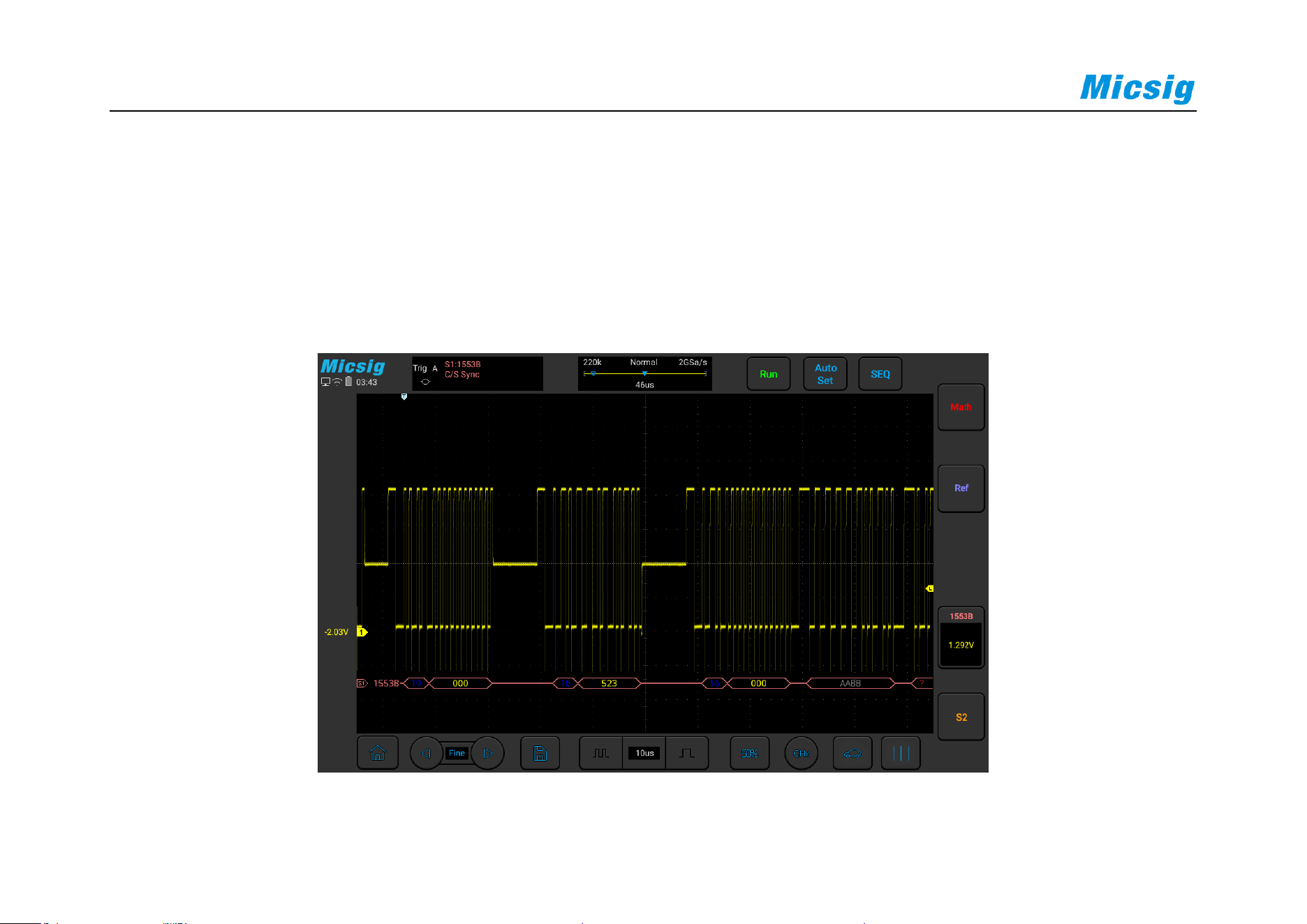
366
(3) Open the trigger setting menu, select the trigger type as bus trigger, 1553B, and trigger mode as
“command/status word sync header”.
Channel threshold level is adjusted according to signal amplitude. 1553B trigger graphic interface is shown in
Figure 12-32:
Figure 12-32 1553B Graphic Interface

Chapter 12 Serial Bus Trigger and Decode (Optional)
367
1553B decode data packet description:
(1) Remote terminal address (5-bit data): blue
(2) The value of remaining 11 bits of the command/status word: yellow
(3) Decoded data: white
(4) If the command/status or data word has a parity error, its decoded text is displayed in red instead of green
or white.
(5) The sync error is displayed together with the word “SYNC”.
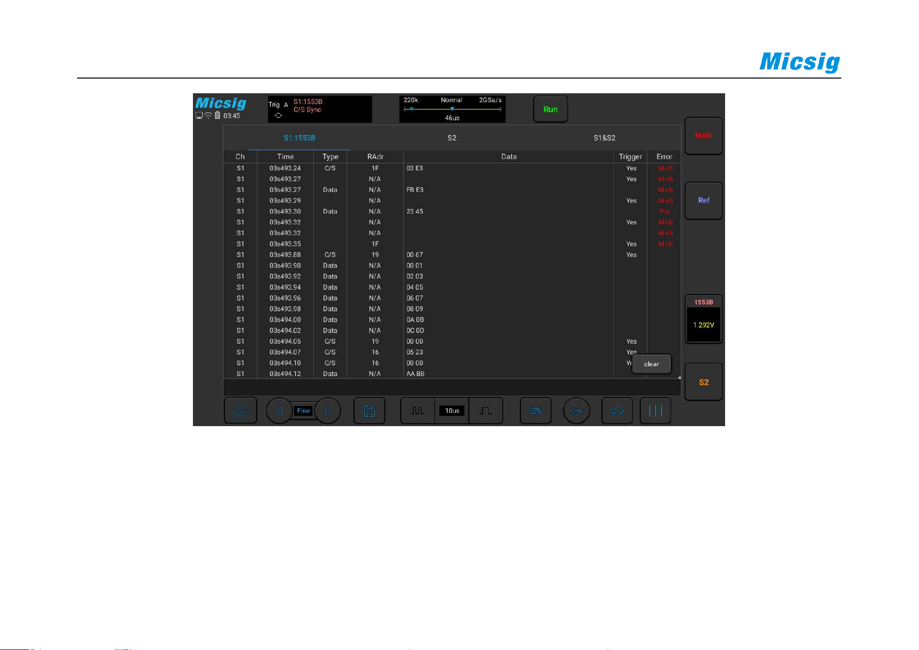
368
Figure 12-33 1553B Text Interface
1553B text interface description, as shown in Figure 12-33:
(1) “Ch”: bus channel.
(2) “Time”: intervals between the last read/write operations to current read/write operations.

Chapter 12 Serial Bus Trigger and Decode (Optional)
369
(3) “Type”: frame type (data frame DATA, command/status frame C/S, others N/A).
(4) “RAdr”: remote terminal address, displayed in the selected numeration system (N/A for no content
display).
(5) “Data”: content of the transmitted information, displayed in the selected numeration system.
(6) “Trigger”: “Yes” means reach trigger condition.
(7) “Error”: displays the frame error type (parity error Par, Manchester coding error M-ch).

370
Chapter 13 Homepage Functions
This chapter contains the functions of the oscilloscope homepage and describes the functions of all icons on the
homepage and settings. You are recommended to read this chapter carefully to understand the homepage functions
of the ATO series oscilloscope.
Oscilloscope
Gallery
App Store
Calendar
Settings
Electronic Tools
File manager
Clock
Calculator
Power Off
Browser
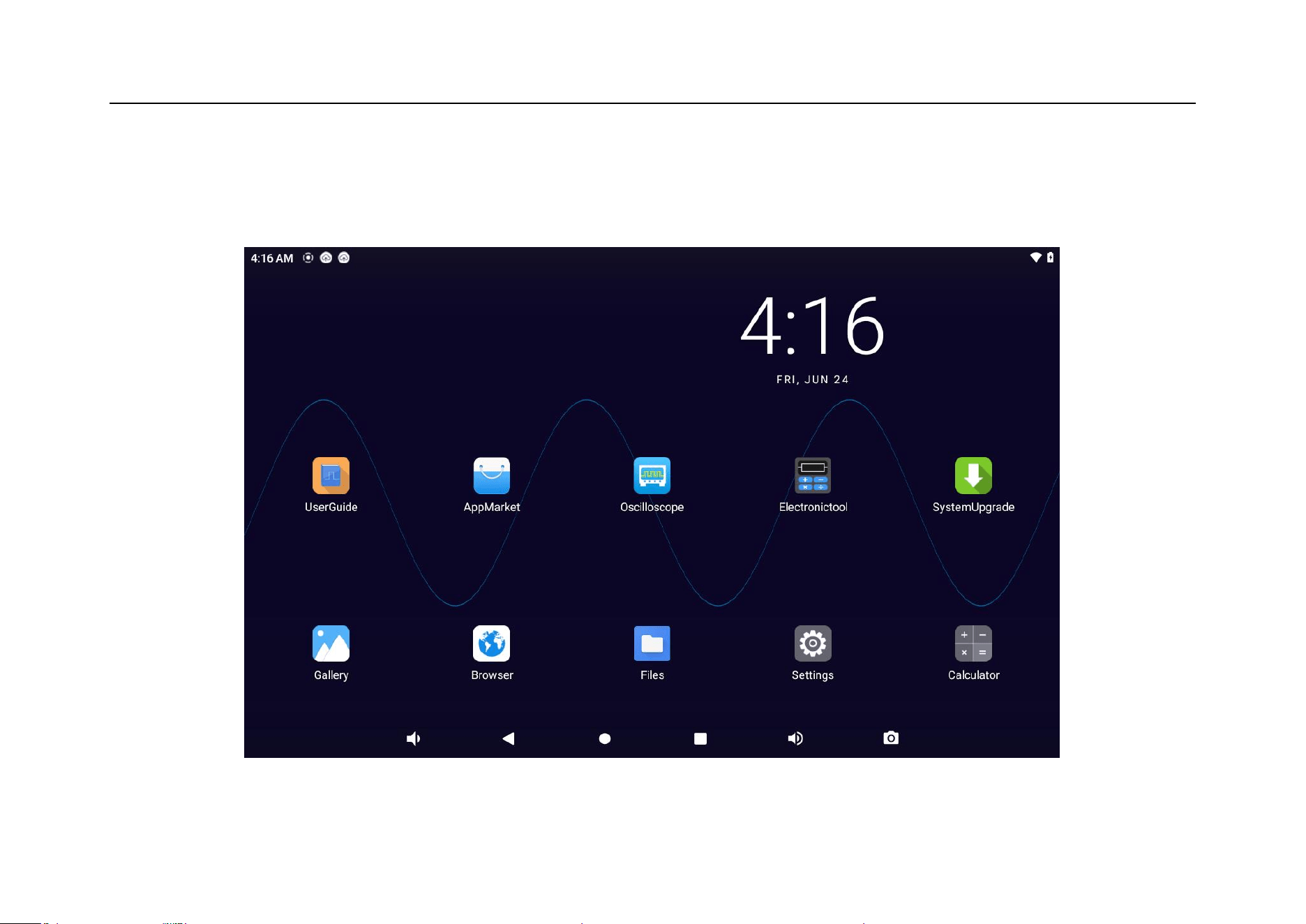
Chapter 13 Homepage Functions
371
The following figure shows the contents of the oscilloscope home page. Slide left or right to display the remaining
applications. See Figure 13-1.
Figure 13-1 Homepage Interface
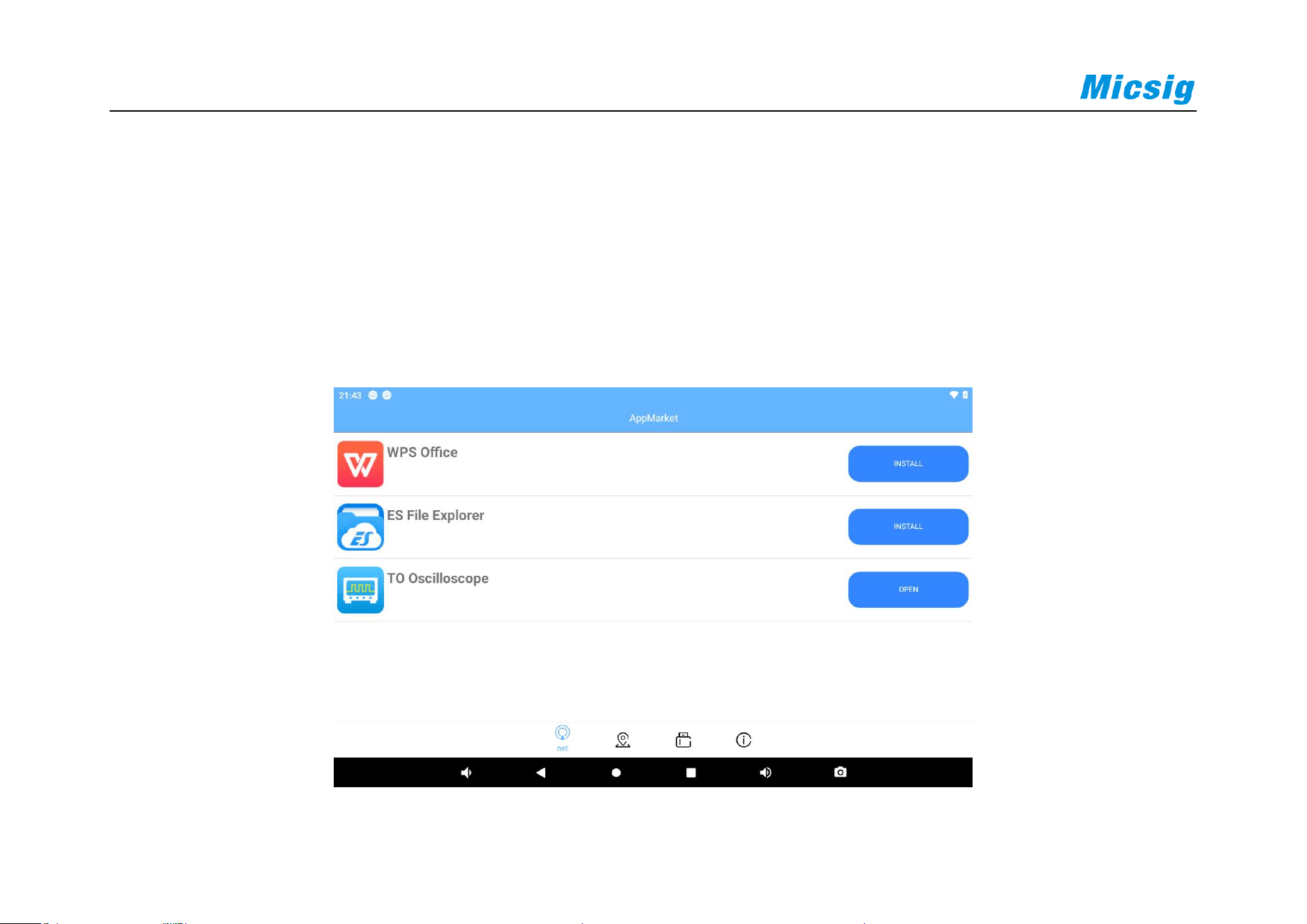
372
13.1 Oscilloscope (see Chapters 2~12)
13.2 App Store
Tap the app store icon on the homepage to go to the app store interface, as shown in Figure 13-2. App store content
includes Network, Local, U-disk, and About.
Figure 13-2 App Store

Chapter 13 Homepage Functions
373
Network
Tap “Network” to open the application list.
Tap app icon to view details such as version number of the current app and app description, and tap the green open
option below to open or install the current app.
Tap the green option on the right of the app list to open and install the app.
Local
Apps that have been downloaded and installed are displayed locally. When there is no downloaded application
installation package file locally, the interface will display “There are no available apk files in the local directory”.
U-disk
The U disk interface will display applications that can be opened in the USB disk.
If the USB disk is not plugged, the interface displays “U-disk not inserted”.

374
After USB disk has been plugged, if there are no apk files in the USB device for installation, the interface displays
“There is no available apk file in the U disk directory”.
About
In “About” interface, the equipment model, bandwidth, serial number, version information, shipment date and
information about installed options can be viewed. Open the virtual keyboard and enter the license to install the
corresponding options.
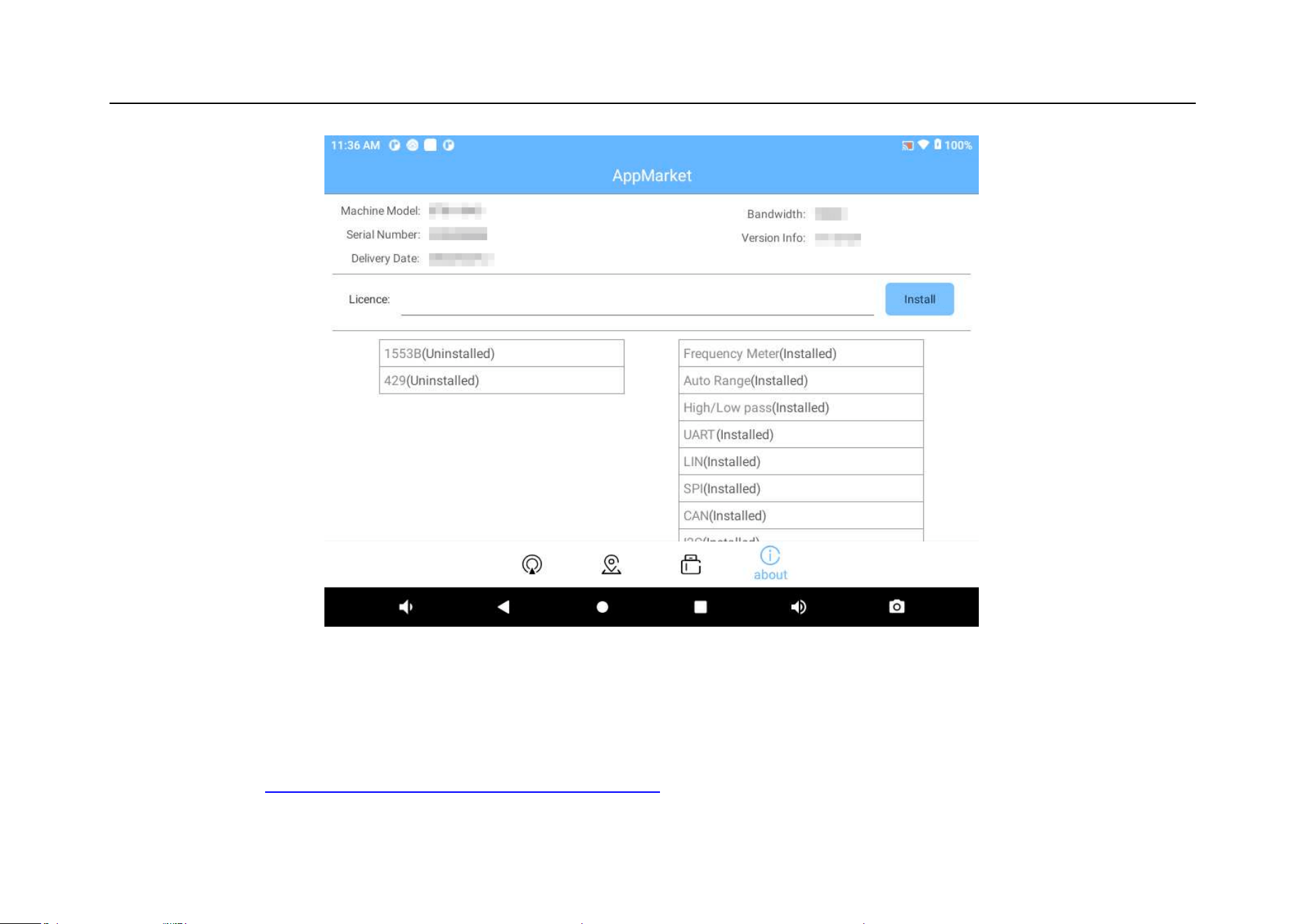
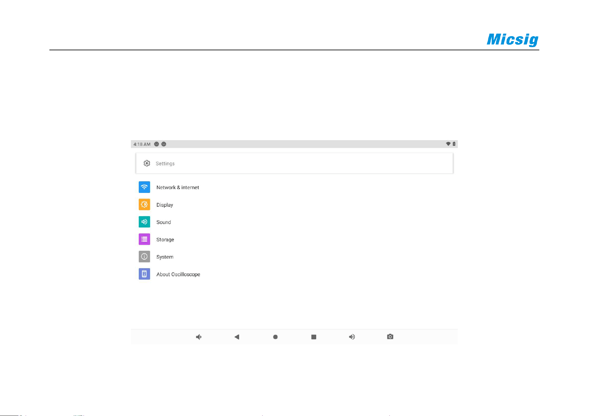
376
13.3 Settings
Tap settings on Homepage to enter the System Settings interface. Settings on the settings interface include Network
& internet, display, sound, storage, system and About Oscilloscope, as shown in Figure 13-4.
Figure 13-4 System Setting Interface
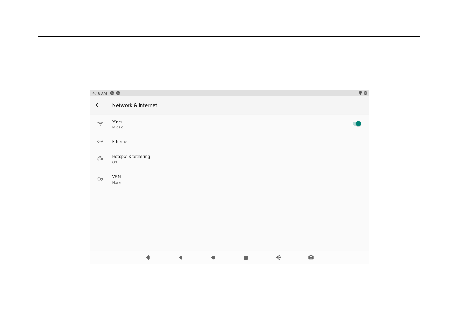
Chapter 13 Homepage Functions
377
WLAN connection
Tap WIFI icon to enter the WLAN settings interface, as shown in Figure 13-5.
Figure 13-5 WLAN Connection Setting

378
Tap on/off bar to turn the WLAN function on. Oscilloscope can automatically scan the surrounding wireless
networks and display their names by list.
Tap the wireless network to be connected and the password input box will pop up. After entering password using
the virtual keyboard, tap Enter to connect oscilloscope to the wireless network.
Click the current network can advanced settings for WIFI.
Portable WLAN hotspot
Tap Hotspot to enter the portable hotspot settings interface.
Tap the off icon to open the hotspot. Click “hotsopt name” to enter the network name and password using the
virtual keyboard, as shown in Figure 13-6. Other equipment can share oscilloscope files by linking oscilloscope
hotspots (portable hotspot default IP is: 192.168.243.155).
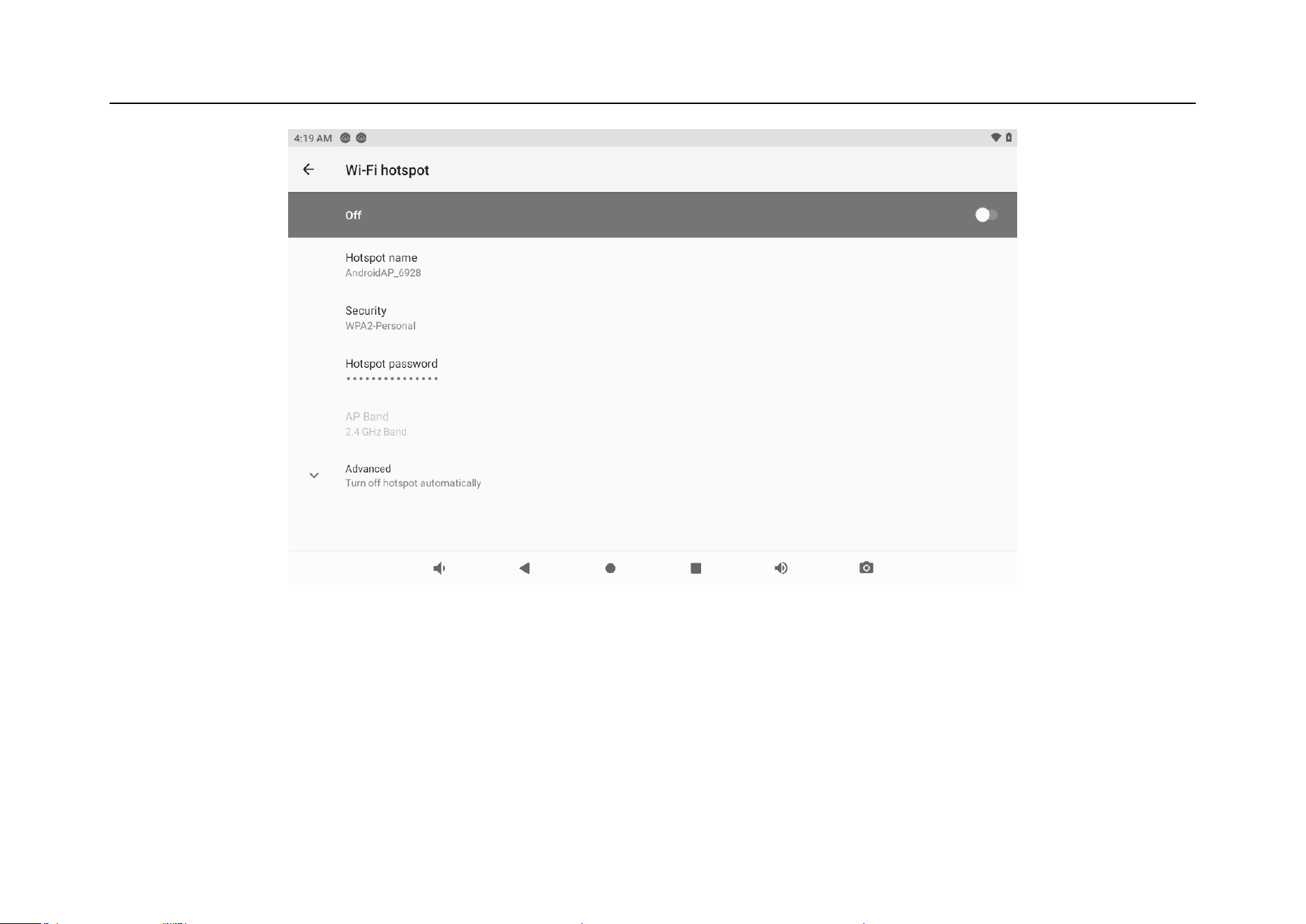
Chapter 13 Homepage Functions
379
Figure 13-6 Portable WLAN Hotspot Setting
Display
Tap display icons to set the oscilloscope Brightness level, Dark theme, Wallpaper, Font size and Display size.
Brightness level: The progress bar can be dragged to set the brightness of the screen display.

380
Dark theme: Set Dark theme uses a black background to help keep battery alive longer on some screens.
Wallpaper: Set the screen wallpaper.
Font size: Change the system display font size.
Display size: Make the items on your screen smaller or larger. Some apps on your screen may change position.
Sound
Tap the “sound” icon and drag the progress bar in the sound section to change the media volume, alarm volume and
notification volume. After clicking the default notification ring tone, drag up and down to select the ring tone, then
click OK.

Chapter 13 Homepage Functions
381
Storage
Tap storage to enter the storage space view interface, then view the total storage capacity, size of available space, as
well as memory size of applications (application data and media content), pictures, videos, audio (music, ringtones,
podcasts, etc.), download content, cache data, and others.
If USB device is plugged, it will display the total storage capacity and available memory size, and can also uninstall
and format SD card.
Language and input method
Tap System →language & input icons to set your system language and input method.
Language: add a language and drag it to the first position of language list to make it as system language.
Spell Checker: When this function is turned on, it will automatically check for correctness as you type.

382
On-screen keyboard includes Android keyboard and Gboard, tap +manage on-screen keyboards to turn off one of
them.
Advanced setting include Spell checker, Autofill service, Personal dictionary, Pointer speed.
Date and time
Tap System →Date & time icons to set your system date and time
Use network-provided time: When turned on, the time provided by the network will be used as the system time.
Date and time cannot be set manually after turning this on.
Set date: Set the system date manually.
Set time: Set the system time manually.
Select time zone: Set the time zone manually.
Use 24-hour system: If on, the system time will be 24-hours, and off for 12 hours.

Chapter 13 Homepage Functions
383
About Oscilloscope
In the “About” interface, view legal information, Android version, IP address, build number and other information.
Accept online updates: turn off/on System update, app update, boot interface update, userguide update ...
13.4 File Manager
File manager app can enable quick access to and management of various files stored on the equipment.
Tap the Files app icon on the homepage screen to enter the file manager interface.
Recent: shows files that have been opened recently
Classification: views files by types, including images, videos, Audio, Documents, Downloads, STO etc.

384
Local: views the content stored in the oscilloscope by the traditional folder list mode. When USB device is plugged,
the content in the USB device can also be accessed through external storage.
To operate files, simply press and hold a single file to select it. The selected file will show blue √. Then, click the
remaining files to select them. If all files must be selected, tap theicon at the right top of the screen and click
Select all, which also includes copy, cut, compress, rename and more operations. Tap the trash icon to delete files.
13.5 Calculator
Tap calculator icon on the homepage to open the calculator app.
Calculator can perform simple addition, subtraction, multiplication and division calculations as well as scientific
calculations.
13.6 Browser
Tap the browser icon on homepage interface to enter the browser interface, and then it can access to the internet if
the network condition is good, as shown in Figure 13-7.
Chapter 13 Homepage Functions
385
Figure 13-7 Browser Interface
13.7 Gallery
Tap gallery application on the homepage interface to enter the picture viewing interface, as shown in Figure 13-8.
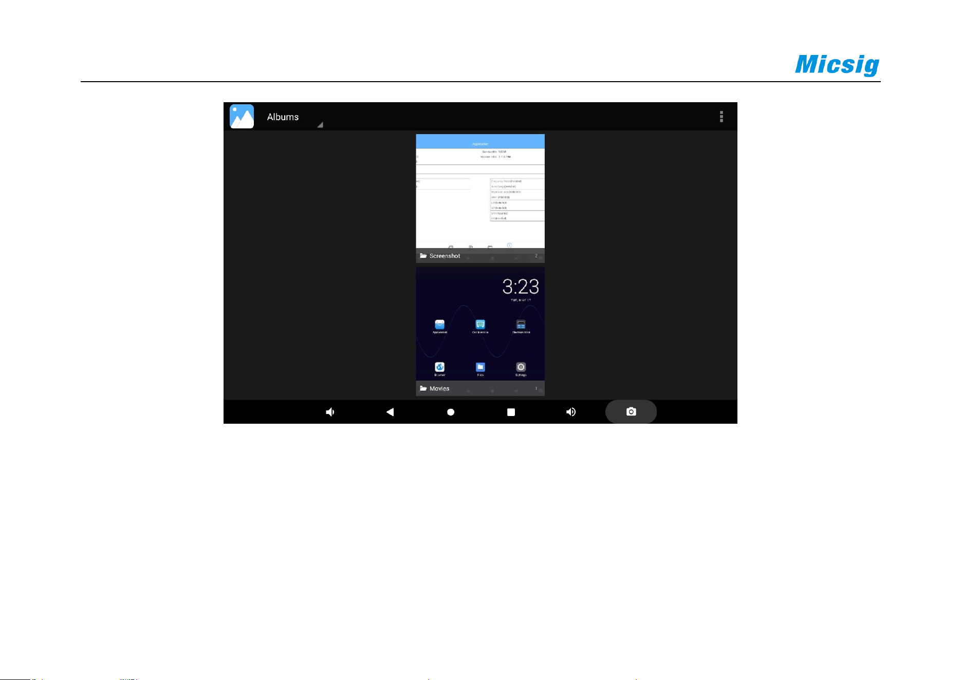
386
Figure 13-8 Picture Viewing Interface
Gallery provides locally stored photos/videos with the functions of picture/video viewing and photo editing.
In the picture view interface, pictures and videos can be classified into different categories according to the method
in the upper left corner, and tap them to view pictures or videos.
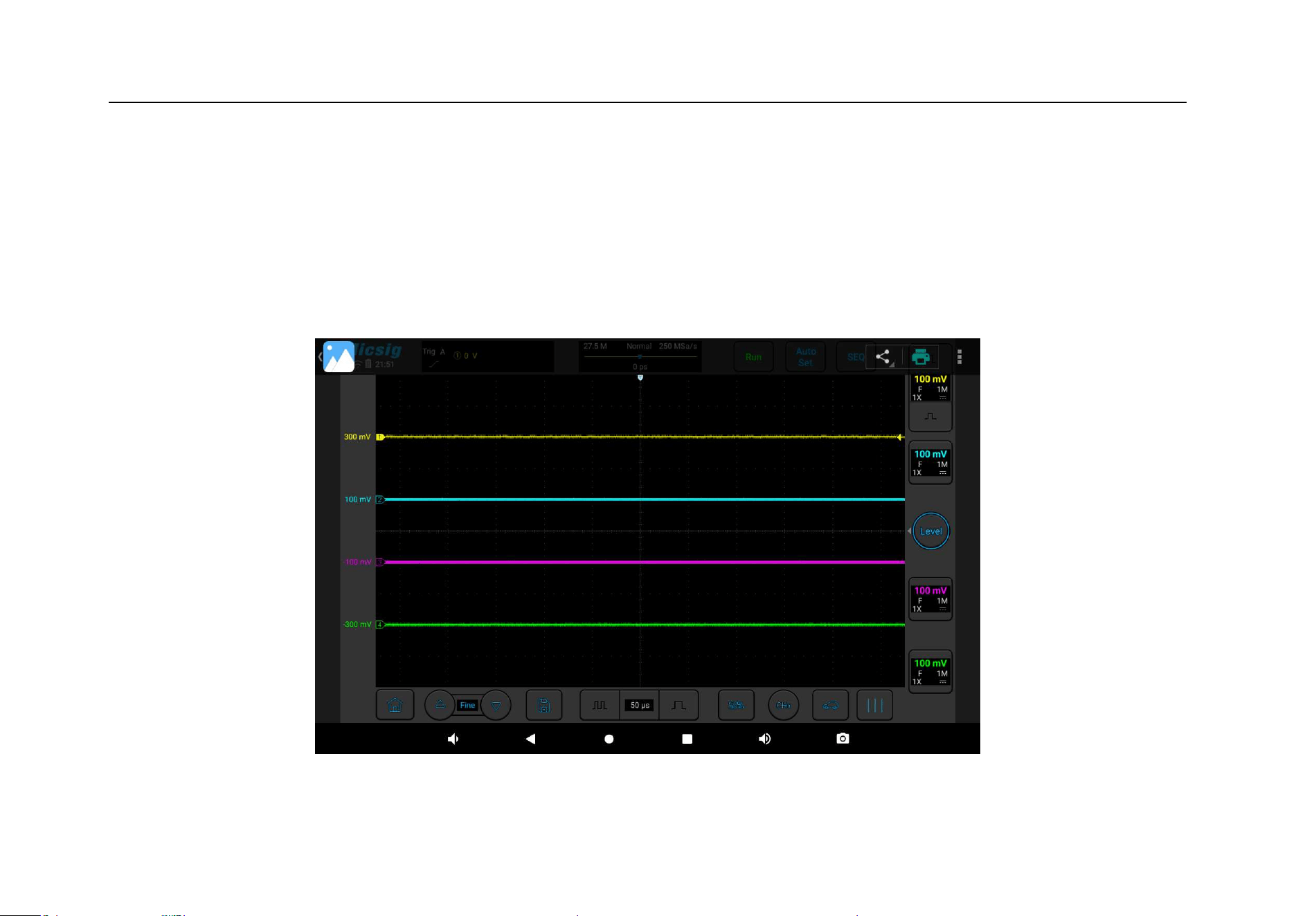
Chapter 13 Homepage Functions
387
When viewing pictures, click to display them in full screen. When viewing videos, swipe left and right to select the
video you want to play. Click the triangle play button, and the video will play automatically. Tap the screen to pause
play. Drag the pictures left and right when displaying in full screen to view previous and next pictures. Tap the back
button to exit the full screen display, as shown in Figure 13-9.
Figure 13-9 Full-Screen Picture Viewing Interface

388
When viewing pictures and videos, tap the option at the top right of the screen and click to select items. The
pictures and videos can be selected. Click the recycle bin icon in the upper right corner of the screen to delete
pictures or videos.
After the USB device is connected to oscilloscope, if there are pictures or videos in the USB device, they will be
automatically displayed on the picture viewing interface.
13.8 Calendar
Tap the calendar app icon on the homepage to enter the calendar interface.
Tap TODAY at the top right of the screen to navigate directly to today's date.
Tap the date at the top left of the screen to adjust the calendar display style by day, week and month.
13.9 Electronic Tools
Electronic tools can provide a convenient set of electronic calculation tools.
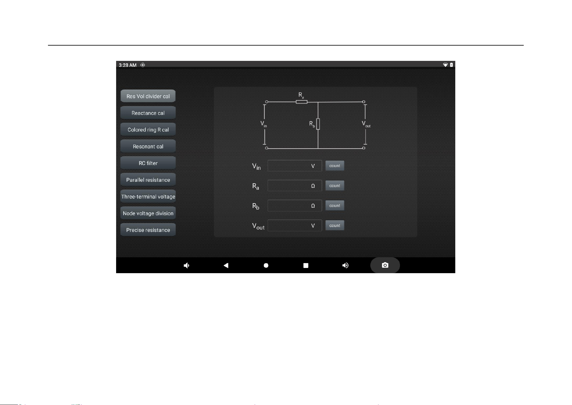
Chapter 13 Homepage Functions
389
Figure 13-10 Electronic Calculation Tool Function
13.10 Clock
Tap time icon on the homepage or tap clock app icon to enter the clock settings screen, as shown in Figure 13-11.

390
Alarm clock
Add an alarm: Click “+” button below to add an alarm clock and create settings.
Alarm time: Drag pink dot in the dial to set the hour, and drag again to set the minute.
Repeat: Monday to Sunday available and click calendar icon on the right to enter the calendar for custom selection.
Alarm ringtone: Select alarm ringtone, support local ringtone, system ringtone, none.
Label: The alarm will be displayed on the screen when it rings.
Delete alarm: Click the alarm to be deleted in the list and select “delete” at the bottom of the alarm edit page.
Switch status: Click the switch behind the alarm to turn it on and off.
World clock
Add region: Click the bottom globe button and select city in the list of cities.
Timer
Add timer: Enter the hour, minute and second, click the triangle button to start countdown.

Chapter 13 Homepage Functions
391
Delete timer: Click “DELETE” to delete the timer.
Pause: Click the double rectangle button to pause timer.
Stopwatch
Start: Click “Triangle” to start timing.
Pause: Click “Double Rectangle” below to pause the stopwatch.
Mark: Click the LAP to mark it.
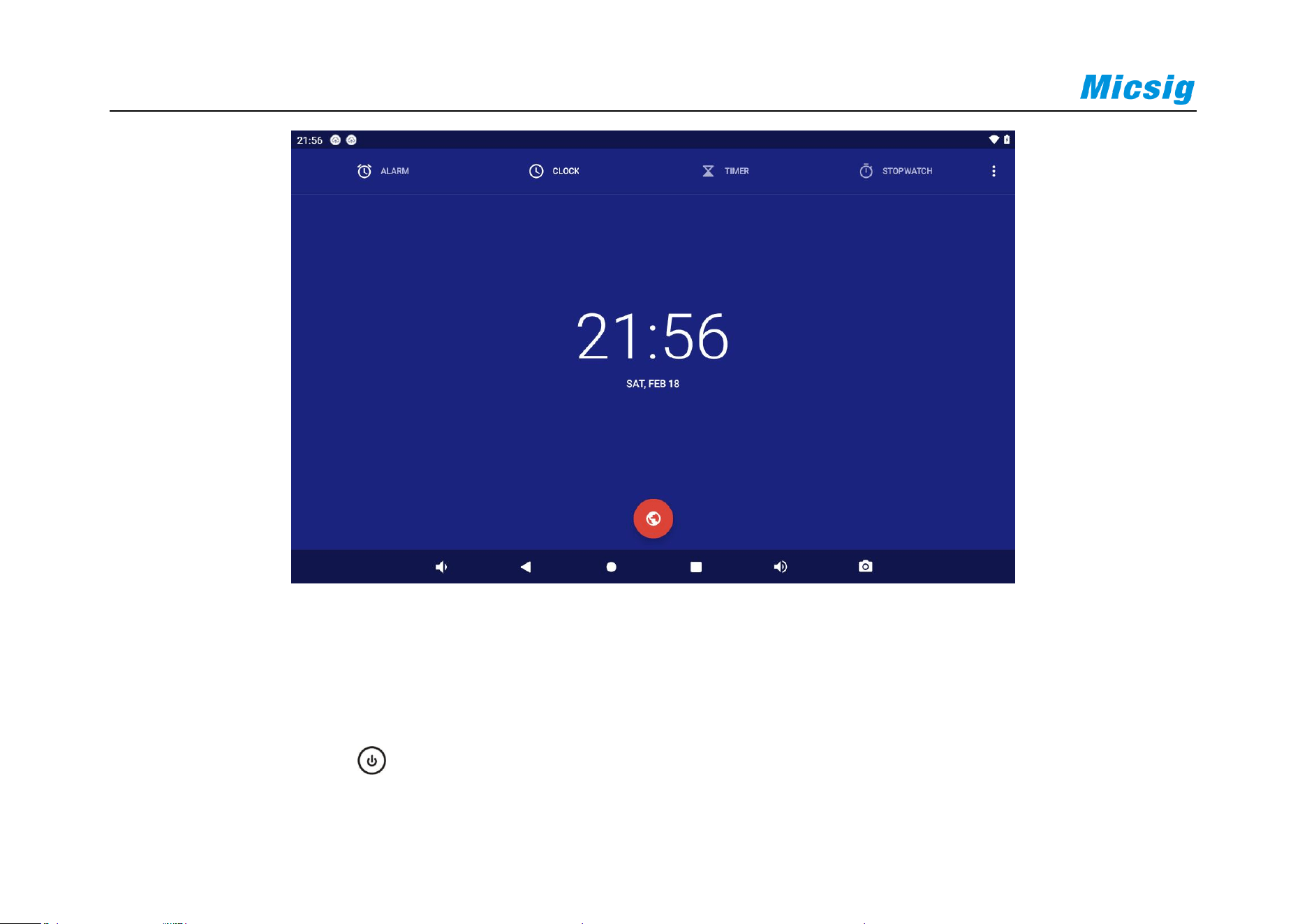
392
Figure 13-11 Time Setting
13.11 Power Off
Long press power button to enter the power off interface, as shown in Figure 13-12. Power off contains 4
options: Shutdown, Reboot, Standby, Lock Screen.
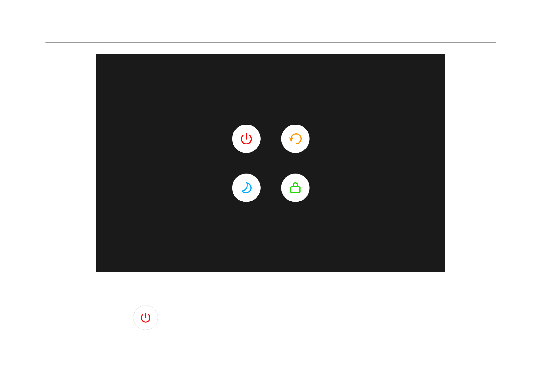
Chapter 13 Homepage Functions
393
Figure 13-12 Power Off Interface
Shutdown: Click the button to turn off the oscilloscope.

394
Reboot: Click the button to restart the oscilloscope.
Standby: Click the button to standby the oscilloscope, press power button to wake.
Lock Screen: Click the button to lock the oscilloscope screen, repeat the step to unlock.

Chapter 14 Remote Control
395
Chapter 14 Remote Control
This chapter contains the application of host computer, mobile remote control, in order to understand remote control
functions of the ATO series oscilloscope.
Host computer
Mobile remote control

396
14.1 Host Computer
To control the instrument using the host computer software, you need to install the NI driver first, then the
RemoteDisplay software is downloaded and installed. This software is only suitable for Micsig ATO series
oscilloscopes.
14.1.1 Installation of Host Computer Software
Note: The host computer software only supports Win7 or higher edition operating system. The computer needs to
install NI-VISA driver first.
The host computer and needed NI-VISA driver can be downloaded from Micsig offical website:
http://www.micsig.com
Download the host computer software on official website of Micsig, open RemoteDisplaySetup.exe file, and
complete the software installation.
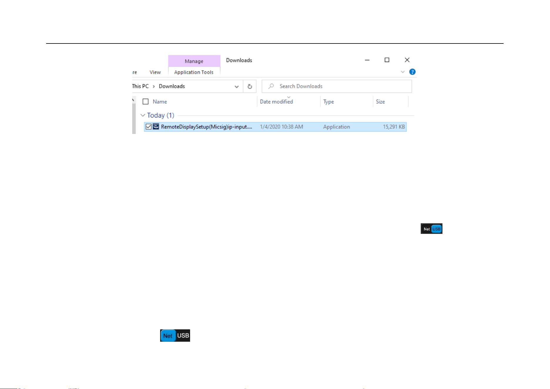
Chapter 14 Remote Control
397
Figure 14-1 RemoteDisplay Software
14.1.2 Connection of Host Computer
USB connection: Connect USB Device to the computer and oscilloscope through USB data cable. After the
computer recognizes the USB device, open the host computer, set the connection mode to USB , and display
the device information in the device information display box in the lower right corner. This indicates that the
oscilloscope has been found. Click to connect to the selected oscilloscope.
WIFI connection: Under the oscilloscope settings →WLAN menu, choose and connect the same WIFI with the
computer to ensure that the computer and the oscilloscope are in the same network. Open the host computer, set
the connection mode to Net , and display the device information in the device information display box in

398
the lower right corner. This indicates that the oscilloscope has been found. Click to connect to the selected
oscilloscope.
Enter IP connection: In case of network connection (WIFI or LAN), directly type oscilloscope IP to be connected
in the oscilloscope device information display box in the lower right corner, and then click the oscilloscope
connection status button, the host computer will be connected to the oscilloscope corresponding to the entered IP
address.
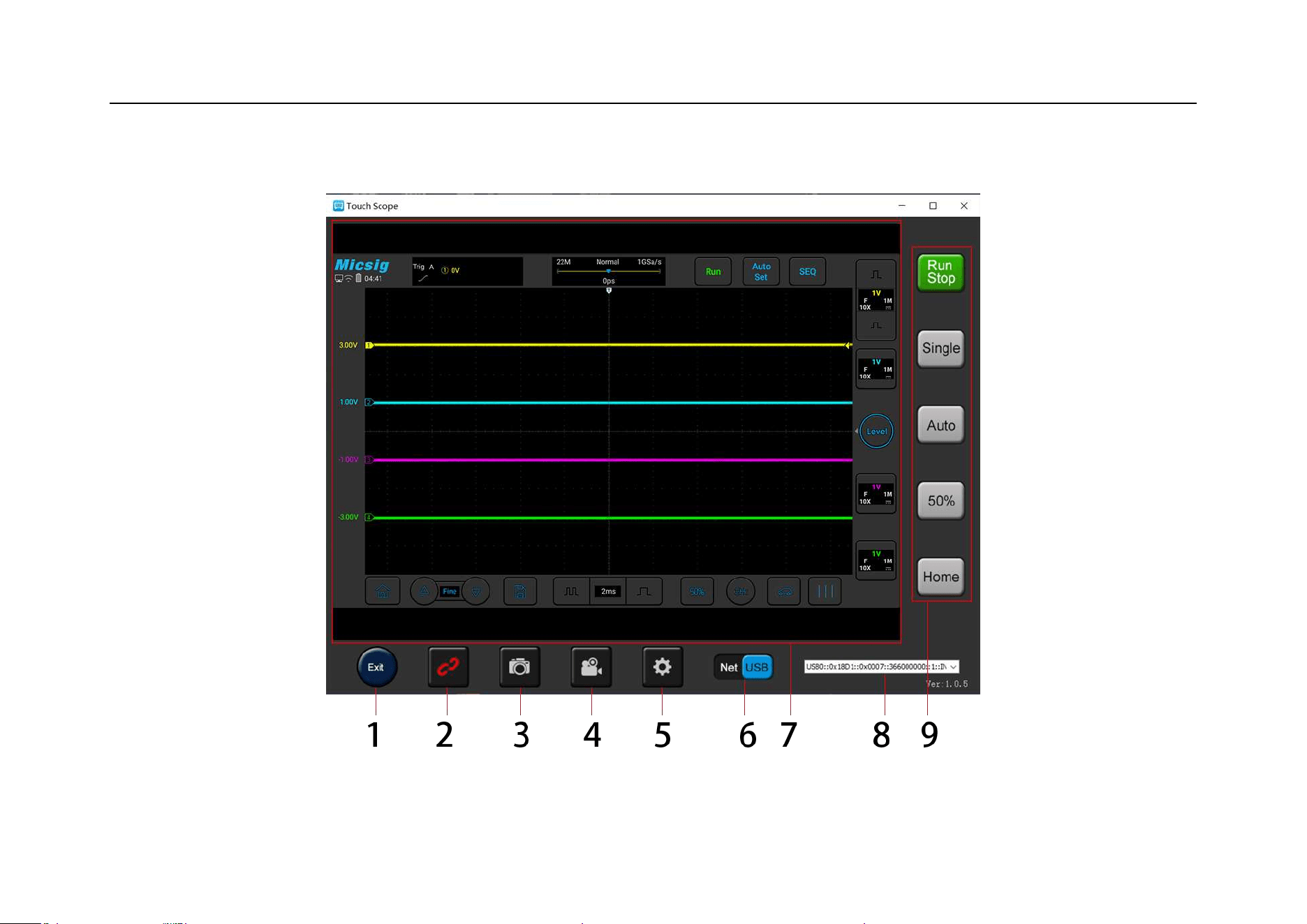
Chapter 14 Remote Control
399
14.1.3 Main Interface Introduction
Figure 14-2 Host Computer Interface

400
1. Host computer on/off button
Click to exit the host computer software
2. Oscilloscope connection status button
The button has two states:
Green: Connect to selected oscilloscope when clicked
Red: Disconnect from oscilloscope when clicked
3. Quick camera button
Click to take photo quickly. Pictures are stored in the local
directory C:\Users\Public\Pictures
4. Video record button
Click to open or close video record function. Videos are stored
in local directory C:\Users\Public\Videos
5. Host computer storage button
Set photo taking and video recording storage locations
6. Select oscilloscope connection
mode
USB and WIFI connections are available

Chapter 14 Remote Control
401
Note: WIFI connection must ensure that oscilloscope and
computer are in the same network
7. Host computer display area
Synchronous display with oscilloscope
8. Oscilloscope information display
Display oscilloscope model, connection mode, SN, IP and other
information, select the oscilloscope to be connected
9. Host computer waveform control area
Waveform control area button has the same function with that
button on the oscilloscope
14.1.4 Operation Interface Introduction
The host computer and the oscilloscope are synchronously displayed, and the waveform operation mode and the
menu opening and closing mode are the same as those on the oscilloscope; the left mouse button and the single
finger operation mode are the same, and both of them can perform the operations of slide, click, drag, etc.
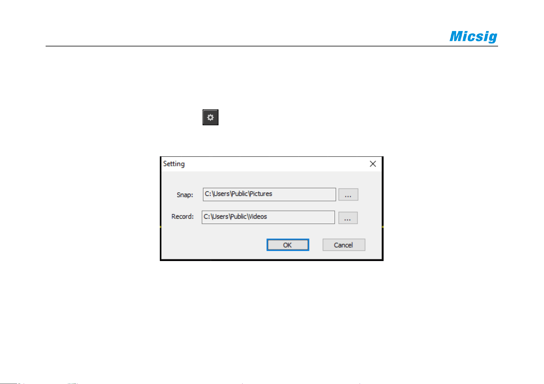
402
14.1.5 Storage and View of Pictures and Videos
Storage setting of pictures and videos:
Open the host computer storage setting , set the storage location of pictures and videos, as shown in the figure
below:
Figure 14-3 Host Computer Storage Setting
Pictures are stored in the local directory C:\Users\Public\Pictures by default. We can also store them under the
directory defined by ourselves according to our own needs. For example, we store pictures in a “mini photo”
directory under E-drive disk. We can set the video storage location in the same way, then click OK.
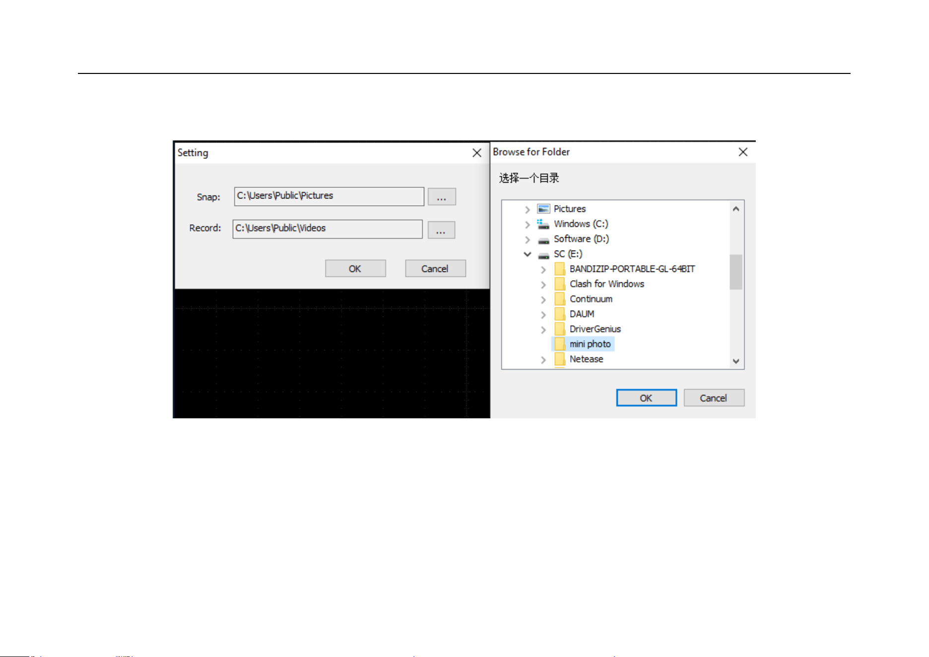
Chapter 14 Remote Control
403
Figure 14-4 Change Storage Directory
View pictures and videos:
Open picture (video) storage directory to view pictures (videos) stored on the host computer.
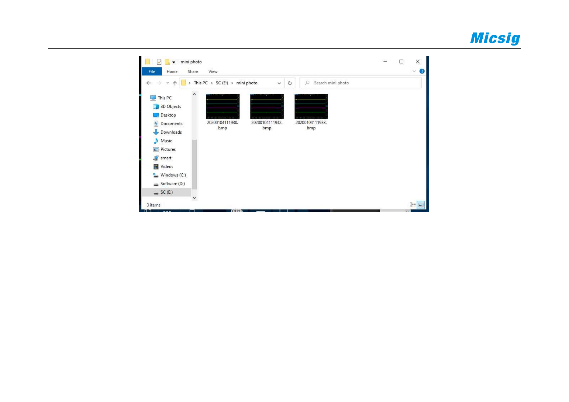
404
Figure 14-5 View Pictures
14.2 Mobile Remote Control
Micsig ATO series oscilloscopes support remote control on mobile phone (android & iOS). You need to download
Android app from the official website of Micsig (address: http://www.micsig.com) and install it. For iOS, go to
apple store search Automotive Oscilloscope or Micsig to get it.
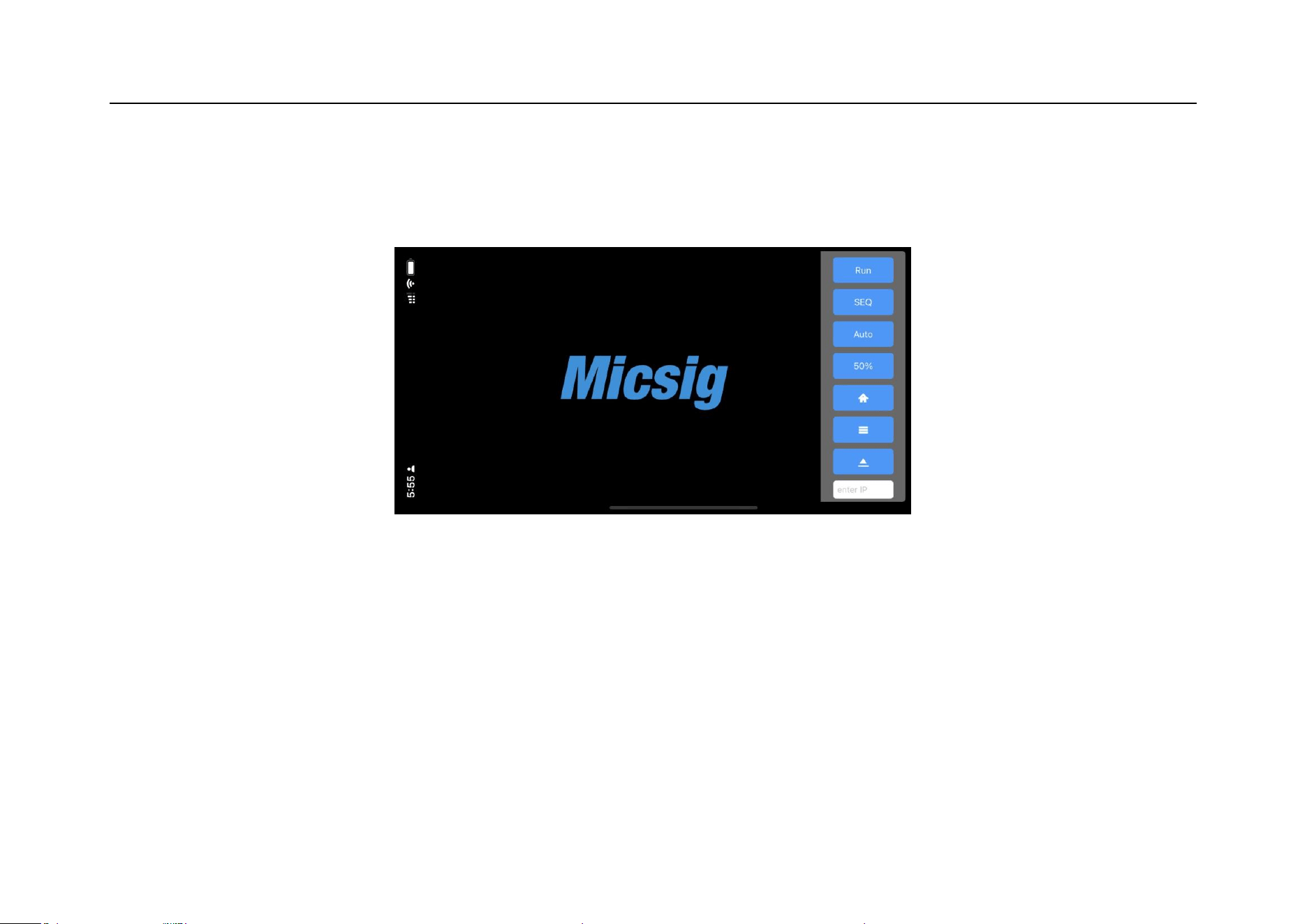
Chapter 14 Remote Control
405
After App is successfully connected, mobile device can be used to control the oscilloscope and display the
oscilloscope interface in a real time manner.
Figure 14-6 APP interface
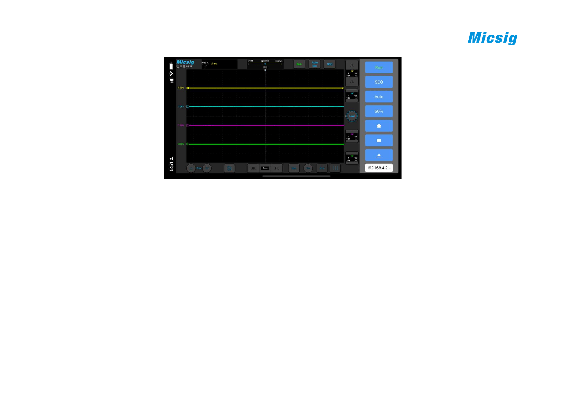
406
Figure 14-7 Successful Connection of APP
Android APP can be connected by two methods:
1. Use oscilloscope portable hotspot: Mobile phone can be connected to the hotspot of oscilloscope. Enter the
oscilloscope IP 192.168.45.1 in the IP box at the lower right corner of the screen to connect successfully for
control;
2. Connect mobile phone and oscilloscope to the network segment under the same router: view the IP address of
the oscilloscope, and enters such IP address in the lower right corner of the mobile phone to connect
successfully.

Chapter 14 Remote Control
407
The first connection method is recommended.

408
Chapter 15 Update and Upgrade Functions
This chapter describes the methods of software update and increasing the optional function. You are recommended
to read this chapter carefully understand the upgrade functions of the ATO series oscilloscope.
Software update
Add optional functions
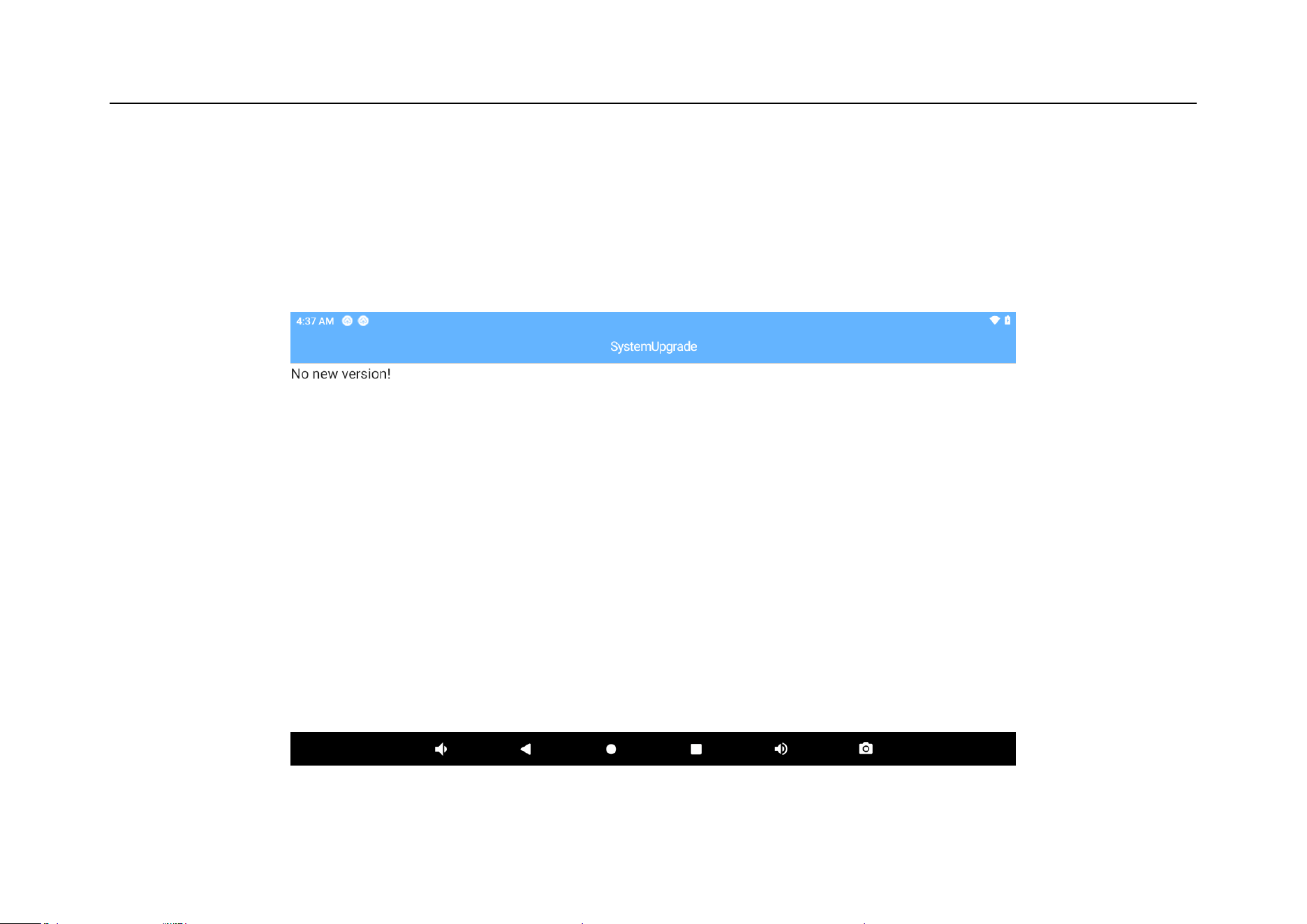
Chapter 15 Update and Upgrade Functions
409
15.1 Software Update
Micsig often releases software updates for its products. To update your oscilloscope software, you can connect the
oscilloscope to WIFI for networking, and open the SystemUpgrade application to check and install update.
Figure 15-1 SystemUpgrade application

410
Note: Please pay attention to keep the oscilloscope power more than 50% when installing updates or connect
the oscilloscope to the adapter, so as to prevent the oscilloscope from becoming abnormal due to insufficient power
for update.
To view the currently installed software and firmware, tap the “App Store” software in the “Home” page to display
the oscilloscope software and firmware information on the “About” screen. Please refer to
13.2 App Store.
15.2 Add Optional Functions
Tap the “App Store” software in the “Home” page to display the installed and uninstalled decoded options on the
“About” screen. Please refer to
13.2 App Store.
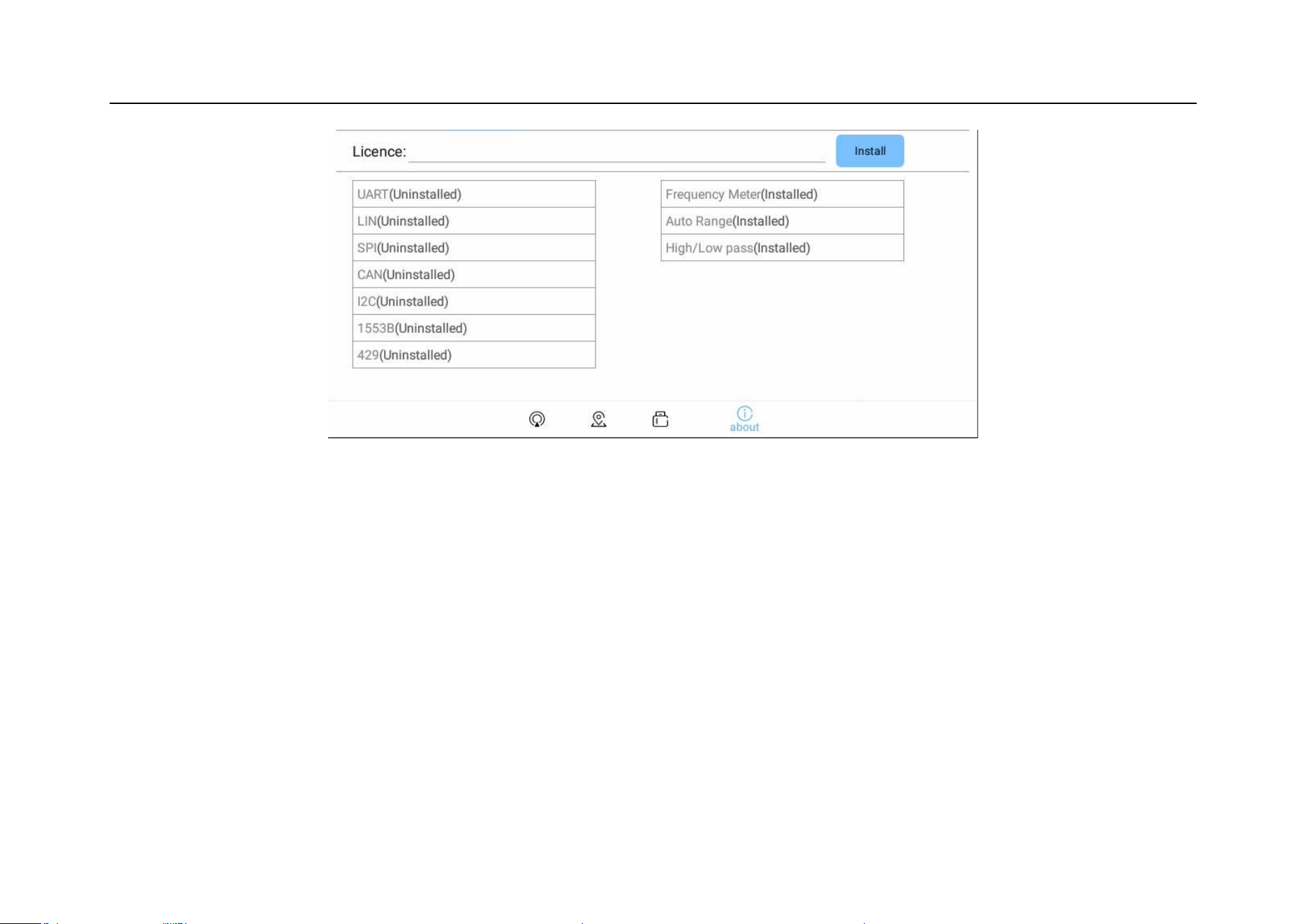
Chapter 15 Update and Upgrade Functions
411
Figure 15-2 Decode Functions Not Installed
If you need the optional function service, please contact Micsig for license and enter the install option function at
the license bar.
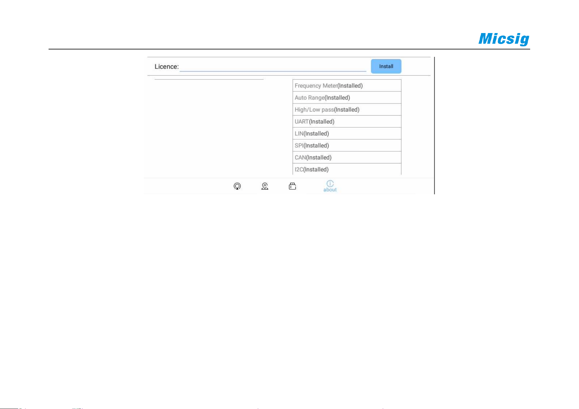
412
Figure 15-3 Decode Functions Installed

Chapter 16 Reference
413
Chapter 16 Reference
This chapter contains the measurement category suitable for the oscilloscope and the environmental level of
pollution degree supported. You are recommended to read this chapter carefully to understand the conditions of use
of the ATO series oscilloscope.
Measurement Category
Pollution Degree

414
16.1 Measurement Category
Oscilloscope measurement category
Smart oscilloscopes are primarily used for measurements in Measurement Category I.
Measurement category definitions
Measurement category I is for measurements performed on circuits not directly connected to MAINS. Examples are
measurements on circuits not derived from MAINS, and specially protected (internal) MAINS derived circuits. In
the latter case, transient stresses are variable; for that reason, the transient withstand capability of the equipment is
made known to the user.
Measurement category II is for measurements performed on circuits directly connected to the low voltage
installation. Examples are measurements on household appliances, portable tools and similar equipment.
Measurement category III is for measurements performed in the building installation. Examples are measurements
on distribution boards, circuit-breakers, wiring (including cables, bus-bars, junction boxes, switches, socket-outlets)

Chapter 16 Reference
415
in the fixed installation, and equipment for industrial use and some other equipment, for example, stationary motors
with permanent connection to the fixed installation.
Measurement category IV is for measurements performed at the power source of the low-voltage installation.
Examples are electricity meters and measurements on primary overcurrent protection devices and ripple control
units.
Transient withstand capability
Maximum input voltage of the analog input
Category I 300Vrms, 400Vpk.
16.2 Pollution Degree
Pollution Degree
ATO series oscilloscopes can operate in environments with pollution degree 2 (or
pollution degree 1).

416
Pollution Degree
Categories
Pollution degree 1: No pollution or only dry, non-conductive pollution occurs. The
pollution has no influence. For example: a clean room or air-conditioned office
environment.
Pollution degree 2: Normally only dry, non-conductive pollution occurs.
Occasionally temporary conductivity caused by condensation may occur. For
example: general indoor environment.
Pollution degree 3: Conductive pollution, or dry, non-conductive pollution occurs
which becomes conductive due to condensation. For example: sheltered outdoor
environment.
Pollution degree 4: Pollution that generates persistent conductivity through
conductive dust, rain, or snow. For example: outdoor locations.

Chapter 17 Troubleshooting
417
Chapter 17 Troubleshooting
1. If the oscilloscope does not start up at power on, please follow steps below:
Check the power cord to verify whether it has been connected properly and whether the power supply is
normal;
Check the power on/off buttons to ensure it has been pushed, and if you are using battery, check whether
the battery is in good condition;
Check the Power-off lock on the side of oscilloscope;
Contact Micsig if the problem persists, and we will provide service to you.
2. If acquired waveforms do not display on the screen when the signal source is connected, please follow
the steps below:
Check whether the probe is connected correctly in the BNC socket;
Check whether the probe is connected correctly in the signal source;

418
Check whether the trigger type is correctly selected;
Check whether trigger conditions are set correctly
Check whether signal source is working properly;
Check whether the channel is turned on;
Check whether the vertical scale factor is set correctly;
Check whether the instrument is in single-sequence waiting state for trigger
Tap to resample signal.
3. If the measured voltage amplitude is 10 times greater or smaller than the actual value:
Check whether the set attenuation factor of the channel is consistent with the attenuation factor of the
actually used probe.
4. There is a waveform display, but cannot be stable:

Chapter 17 Troubleshooting
419
Check the trigger source on the trigger type menu to ensure that it is consistent with the actually used signal
channel;
Check the trigger type: edge trigger is adopted for general signal, and video trigger mode for video signal.
Only the correct trigger mode is used, the waveform can be displayed stably;
Check signal source noise. Set the trigger coupling mode to be high-frequency rejection or low-frequency
rejection to filter out high frequency or low frequency noise interference
5. A waveform is displayed but inconsistent with the input waveform:
Check whether the coupling mode setting in the channel menu is correct.
6. If there is no display after pressing or button:
Check whether the trigger mode is “Normal”, and whether the trigger level is beyond the scope of the
waveform. Center the trigger level and set the trigger mode as “Auto”.
Check whether the picture is displayed in full screen, and if so, exit the display.

420
7. If the display becomes slower after setting average times of sampling:
If the average times are above 32, it is normal for the general speed to become slow.
You can reduce the average times.
8. Staircase waveform is displayed:
This phenomenon is normal because the horizontal time base is too low, and the horizontal time base may be
increased to raise the horizontal resolution, and then improve the display;
The display type may be “line”. The connection between sampling points may lead to the display of
staircase waveform. This problem can be solved by setting the display type as “point” display mode.
9. There is persistence of vision in waveform display:
This phenomenon is normal because the persistence time may be set too long, and the waveform persistence
shows persistence of vision;
The reason may be that sampling mode is set to envelope of sampling, and the sampling mode can be
modified to normal waveform for normal display

Chapter 17 Troubleshooting
421
10. During measurement, the measured value is displayed as -----:
This phenomenon is normal. When the channel waveform displays beyond the waveform display area, the
measured value is displayed as -----. If the channel vertical sensitivity or vertical position is adjusted, the
measured value can be displayed correctly;
This phenomenon is normal. When there is no full-cycle waveform in the waveform display area, the
measured value may be displayed as -----. If the time base is adjusted, the measured value will be displayed
correctly.
This phenomenon is normal, and the measured value of the FFT waveform is displayed as -----.
11. CSV files cannot be selected when loading reference:
CSV files are not the supported format that can be loaded into reference channels.
12. Tap the button during the use of oscilloscope, there is no beep sound:
Check whether the sound volume setting is correct.

422
13. Oscilloscope backlight has low brightness:
Check whether the backlight settings are correct.
14. A waveform being moved changes abruptly:
Check whether the picture is displayed in full screen.
15. Turn off the channel at Auto state:
This phenomenon is normal. At Auto state, the channel with an amplitude less than 10mV will be turned off.
16. Function buttons are pressed without response:
Check whether the picture is displayed in full screen.

Chapter 18 Services and Support
423
Chapter 18 Services and Support
Service Commitments : Micsig guarantees that the products are manufactured and tested according to national
standards or enterprise standards, no unqualified products will leave our factory and the first-class customer
services are provided for all sold products. The warranty period for our products is three years since date of
shipment, and six months for the sold spare parts and the product repair and maintenance. For the details of
warranty service, please read the “Scope of Limited Warranty and Services” chapter. Micsig provides lifetime repair
and maintenance services for products. In accordance with the relevant provisions of after-sale service of industrial
products and the enterprise’s own capacities, Micsig commit as follows:
Repair Commitments : Micsig commits to use the original factory parts for products returned by the user for
repair (under warranty or not) and the commissioning and testing standards are identical with new products. Micsig
the obligation to inform the customer, but without any other obligations for non-product defects or products with
decreased performance not for objective reasons.

424
Service Time Commitments : Micsig will give a reply of the time and cost for repair within 2 working days after
receiving the product returned by the user for repair. After the reply is confirmed, the repair period for a general
fault is 5 working days and shall not exceed 10 working days for any special fault.
Contact us
Shenzhen Micsig Technology Co., Ltd.
Address: 1F, Bldg A, Huafeng International Robot Industrial Park, Hangcheng Rd, Bao'an District, Shenzhen,
Guangdong, China
Tel: (0755)-8860-0880
Website:
www.micsig.com
Email: [email protected]
Postal Code: 518126

Annex
425
Annex
Annex A:Maintenance and Care of Oscilloscope
General maintenance
Do not put or leave the instrument in a place where the LCD display will be exposed to direct sunlight for
long period.
Caution: To avoid damage to the oscilloscope or probes, do not expose them to sprays, liquids, or solvents.
Clean oscilloscope
Examine the oscilloscope and probes as often as operating conditions require. To clean the exterior surface, perform
the following steps:
Use a soft cloth to remove floating dust on the outside of the oscilloscope and probes. Take care to avoid
scratching the touch screen while cleaning.

426
Use a soft cloth dampened with water to clean the oscilloscope while doing this please keep the power off. Wipe
with a mild detergent and water. Do not use any corrosive chemical cleaning agent, in order to avoid damaging
the oscilloscope or probe.
Clean the ventilation hole with a soft brush to keep it unimpeded. Do not use any corrosive chemical cleaning
agent, so as to avoid damage to the oscilloscope motherboard.
If the fan needs to be cleaned, please consult the after-sales service personnel, so as to avoid damage to the
oscilloscope.
Warning
Make sure the instrument is dry before recharging, to avoid electrical short circuit or personal injury caused by
moisture.
Store oscilloscope
The lithium battery needs to be charged before storing the oscilloscope for a long period.
Battery charge

Annex
427
Upon delivery, the lithium battery may not be charged. It takes 6 hours to be fully charged (the oscilloscope is
recommended to turn off to save the charging time). When running on battery power, the battery level indicator in
the lower right corner of the screen will indicate the battery usage.
Caution: In order to avoid charging battery from overheating, do not use beyond the permitted environmental
temperature value given in the technical specification.

428
Annex B: Accessories
Standard accessories
1) 2 pcs for 10X standard probes (incl. grounding nut, grounding crocodile clip, standard rubber plug)
2) 4 x BNC banana lines (4CH);
3) 4 x alligator clips (4CH);
4) 4 X Flexible needle (4CH);
5) Power adapter (12V DC, 4A)
6) Power cord
7) Smart calibration certificate
8) Smart packing list

Annex
429
Optional accessories
1) Oscilloscope suitcase/handbag
2) Battery
3) High voltage probe
4) Differential probe
5) Current probe

430
This manual is subject to change without notice.
The contents of this manual are considered correct. If the user finds any error or omission, please contact
Micsig.
The company will assume no responsibility for accident or hazard caused by the improper operation of the
user.
The copyright of this manual shall belong to Micsig. Any organization or individual may not duplicate, copy
or excerpt the contents without Micsig’s authorization. Micsig reserves the right to claim against such
actions.