BEFORE USING THE CALCULATOR
FOR THE FIRST TIME...
This calculator does not contain any main batteries when you purchase it. Be sure to perform
the following procedure to load batteries, reset the calculator, and adjust the contrast before
trying to use the calculator for the first time.
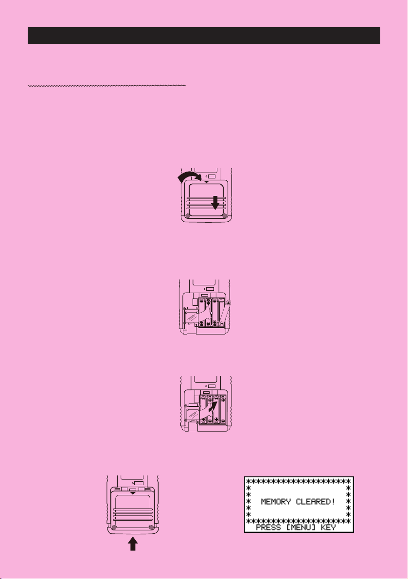
1. Remove the back cover from the calculator by pressing it in the direction indicated by
arrow 1, and then sliding it in the direction indicated by arrow 2.
2. Load the four batteries that come with calculator.
• Make sure that the positive (+) and negative (–) ends of the batteries are facing correctly.
3. Remove the insulating sheet at the location marked “BACK UP” by pulling in the direction
indicated by the arrow.
4. Replace the back cover onto the calculator and turn the calculator front side up, which
should automatically turn on power and perform the memory reset operation.
i
BACK UPBACK UP
MAIN
P
BACK UP
MAIN
P
MAIN
P
P
1
2

ii
5. Press m.
If the Main Menu shown to the right is not on the display,
press the P button on the back of the calculator to perform
memory reset.
6. Use the cursor keys (
f, c, d, e ) to select the CONT icon and press w
or simply press
s
to display the contrast adjustment screen.
7. Use d and e to adjust contrast.
•
d makes figures on the screen lighter, while e makes them darker.
• Holding down
d or e changes the contrast setting at high speed.
8. After adjusting the contrast, press
mto return to the Main Menu.
P
P button
D

KEYS
Alpha Lock
Normally, once you press a and then a key to input an alphabetic character, the keyboard
reverts to its primary functions immediately. If you press ! and then a, the keyboard
locks in alpha input until you press a again.
iii

KEY TABLE
Page Page Page Page Page Page
146
Page Page Page Page Page
151 129
57 56
25756
174 164 136
333 4
2 31333
56 56
56 56
55 55
55 55
24
23
46
46
46
46
49
46
55
46
57
46
59
59
57
46
55
55
25
iv

Switching Power On And Off
Auto Power Off Function
Using Modes
Basic Calculations
Replay Features
Fraction Calculations
Exponents
Graph Functions
Dual Graph
Box Zoom
Dynamic Graph
Table Function
Quick-Start

Quick-Start
vi
Welcome to the world of graphing calculators and the CASIO fx-9750G.
Quick-Start is not a complete tutorial, but it takes you through many of the most common
functions, from turning the power on to graphing complex equations. When you’re done, you’ll
have mastered the basic operation of the fx-9750G and will be ready to proceed with the rest
of this manual to learn the entire spectrum of functions available.
Each step of the examples in Quick-Start is shown graphically to help you follow along
quickly and easily. When you need to enter the number 57, for example, we’ve indicated it as
follows:
Press
fh
Whenever necessary, we’ve included samples of what your screen should look like.
If you find that your screen doesn’t match the sample, you can restart from the beginning by
pressing the “All Clear” button
o
.
SWITCHING POWER ON AND OFF
To switch power on, press o.
To switch power off, press
!
o
OFF
.
AUTO POWER OFF FUNCTION
Note that the unit automatically switches power off if you do not perform any operation for
about six minutes (about 60 minutes when a calculation is stopped by an output command
(^)).
USING MODES
The fx-9750G makes it easy to perform a wide range of calculations by simply selecting
the appropriate mode. Before getting into actual calculations and operation examples, let’s
take a look at how to navigate around the modes.
To select the RUN Mode
1. Press m to display the Main Menu.

Quick-Start
vii
2. Use defc to highlight RUN and then
press
w
.
This is the initial screen of the RUN mode, where you
can perform manual calculations, and run programs.
BASIC CALCULATIONS
With manual calculations, you input formulas from left to right, just as they are written on
paper. With formulas that include mixed arithmetic operators and parentheses, the calculator
automatically applies true algebraic logic to calculate the result.
Example:
15 × 3 + 61
1. Press
o to clear the calculator.
2. Press
bf*d+gbw.
Parentheses Calculations
Example:
15 × (3 + 61)
1. Press
bf*(d
+gb)w
.
Built-In Functions
The fx-9750G includes a number of built-in scientific functions, including trigonometric and
logarithmic functions.
Example:
25 × sin 45˚
Important!
Be sure that you specify Deg (degrees) as the angle unit before you try this
example.

Quick-Start
viii
1. Presso.
2. Press
!
m
SET UP
to switch the set up display.
3. Presscccc1 (Deg) to specify
degrees as the angle unit.
4. Press
J to clear the menu.
5. Press
o to clear the unit.
6. Press
cf*sefw.
REPLAY FEATURES
With the replay feature, simply press d or e to recall the last calculation that was
performed. This recalls the calculation so you can make changes or re-execute it as it is.
Example:
To change the calculation in the last example from (25 × sin 45˚) to (25 × sin 55˚)
1. Press
d to display the last calculation.
2. Press
d twice to move the cursor under the 4.
3. Press
f.
4. Press
w to execute the calculation again.

Quick-Start
ix
FRACTION CALCULATIONS
You can use the $ key to input fractions into calculations. The symbol “ { ” is used to
separate the various parts of a fraction.
Example:
1
15
/
16
+
37
/
9
1. Presso.
2. Press
b$bf$
bg+dh$
jw
.
Converting a Mixed Fraction to an Improper Fraction
While a mixed fraction is shown on the display, press
!
$
d/c
to convert it to an
improper fraction.
Press
!
$
d/c
again to convert back to a mixed fraction.
Converting a Fraction to Its Decimal Equivalent
While a fraction is shown on the display, press M to convert it to its decimal equivalent.
Press
M again to convert back to a fraction.
Indicates 6
7
/
144

Quick-Start
x
EXPONENTS
Example:
1250 × 2.06
5
1. Presso.
2. Press
bcfa*c.ag.
3. Press
M and the ^ indicator appears on the display.
4. Press
f. The ^5 on the display indicates that 5 is
an exponent.
5. Press
w.

Quick-Start
xi
GRAPH FUNCTIONS
The graphing capabilities of this calculator makes it possible to draw complex graphs
using either rectangular coordinates (horizontal axis: x ; vertical axis: y) or polar coordinates
(angle:
θ
; distance from origin: r).
Example
1: To graph Y = X(X + 1)(X – 2)
1. Press
m.
2. Use
d, e, f, and c to highlight GRAPH,
and then press
w
.
3. Input the formula.
v(v+b)
(v-c)w
4. Press 6 (DRAW) or w to draw the graph.
Example
2: To determine the roots of Y = X(X + 1)(X – 2)
1. Press
! 5 (G-Solv).
123456
123456

Quick-Start
xii
2. Press 1 (ROOT).
Press
e for other roots.
Example
3: Determine the area bounded by the origin and the
X = –1
root obtained for Y = X(X + 1)(X – 2)
1. Press
!5 (G-Solv).
2. Press 6 (g).
3. Press
3 (
∫
dx).
4. Use
e to move the pointer to the location where X = –1,
and then press
w. Next, use e again to move the
pointer to the location where X = 0, and then press
w
to input the integration range, which becomes shaded
on the display.
123456
123456

Quick-Start
xiii
DUAL GRAPH
With this function you can split the display between two areas and display two graphs on
the same screen.
Example:
To draw the following two graphs and determine the points of intersection
Y1 = X(X + 1)(X – 2)
Y2 = X + 1.2
1. Press !Zcc1(Grph) to specify
“Graph” for the Dual Screen setting.
2. Press
J, and then input the two functions.
v(v+b)
(v-c)w
v+b.cw
3. Press 6 (DRAW) or w to draw the graphs.
BOX ZOOM
Use the Box Zoom function to specify areas of a graph for enlargement.
1. Press
! 2 (Zoom) 1 (BOX).
2. Use d , e, f, and c to move the pointer
to one corner of the area you want to specify and then
press
w
.
1 23456
123456

Quick-Start
xiv
3. Use d , e, f, and c to move the pointer
again. As you do, a box appears on the display. Move
the pointer so the box encloses the area you want to
enlarge.
4. Press
w, and the enlarged area appears in the in-
active (right side) screen.
DYNAMIC GRAPH
Dynamic Graph lets you see how the shape of a graph is affected as the value assigned to
one of the coefficients of its function changes.
Example:
To draw graphs as the value of coefficient A in the following
function changes from 1 to 3
Y = AX
2
1. Press m.
2. Use
d, e, f, and c to highlight DYNA,
and then press
w
.
3. Input the formula.
aAvxw
123456

Quick-Start
xv
4. Press 4 (VAR) b w to assign an initial value
of 1 to coefficient A.
5. Press
2 (RANG) bwdwb w
to specify the range and increment of change in coeffi-
cient A.
6. Press
J.
7. Press
6(DYNA) to start Dynamic Graph drawing.
The graphs are drawn 10 times.
1 2 3456
↓↑
↓↑
↓

Quick-Start
xvi
TABLE FUNCTION
The Table Function makes it possible to generate a table of solutions as different values
are assigned to the variables of a function.
Example:
To create a number table for the following function
Y = X (X+1) (X–2)
1. Press m.
2. Use
d, e, f, and c to highlight TABLE,
and then press
w
.
3. Input the formula.
v(v+b)
(v-c)w
4. Press 6 (TABL) or w to generate the number
table.
After you’ve completed this Quick-Start section, you are well on your way to becoming an
expert user of the CASIO fx-9750G.
To learn all about the many powerful features of the fx-9750G, read on and explore!
123456

• Your calculator is made up of precision components. Never try to take it apart.
• Avoid dropping your calculator and subjecting it to strong impact.
• Do not store the calculator or leave it in areas exposed to high temperatures or humidity, or large
amounts of dust. When exposed to low temperatures, the calculator may require more time to display
results and may even fail to operate. Correct operation will resume once the calculator is brought back
to normal temperature.
• The display will go blank and keys will not operate during calculations. When you are operating the
keyboard, be sure to watch the display to make sure that all your key operations are being performed
correctly.
• Replace the main batteries once every 2 years regardless of how much the calculator is used during
that period. Never leave dead batteries in the battery compartment. They can leak and damage the
unit.
• Keep batteries out of the reach of small children. If swallowed, consult with a physician immediately.
• Avoid using volatile liquids such as thinner or benzine to clean the unit. Wipe it with a soft, dry cloth, or
with a cloth that has been dipped in a solution of water and a neutral detergent and wrung out.
• In no event will the manufacturer and its suppliers be liable to you or any other person for any damages,
expenses, lost profits, lost savings or any other damages arising out of loss of data and/or formulas
arising out of malfunction, repairs, or battery replacement. The user should prepare physical records of
data to protect against such data loss.
• Never dispose of batteries, the liquid crystal panel, or other components by burning them.
• When the “Low battery!” message appears on the display, replace the main power supply batteries as
soon as possible.
• Be sure that the power switch is set to OFF when replacing batteries.
• If the calculator is exposed to a strong electrostatic charge, its memory contents may be damaged or
the keys may stop working. In such a case, perform the All Reset operation to clear the memory and
restore normal key operation.
• If the calculator stops operating correctly for some reason, use a thin, pointed object to press the P
button on the back of the calculator. Note, however, that this clears all the data in calculator memory.
• Note that strong vibration or impact during program execution can cause execution to stop or can
damage the calculator’s memory contents.
• Using the calculator near a television or radio can cause interference with TV or radio reception.
• Before assuming malfunction of the unit, be sure to carefully reread this manual and ensure that the
problem is not due to insufficient battery power, programming or operational errors.
Handling Precautions
xvii

xviii
Be sure to keep physical records of all important data!
The large memory capacity of the unit makes it possible to store large amounts of data. You should note,
however, that low battery power or incorrect replacement of the batteries that power the unit can cause
the data stored in memory to be corrupted or even lost entirely. Stored data can also be affected by
strong electrostatic charge or strong impact.
Since this calculator employs unused memory as a work area when performing its internal calculations,
an error may occur when there is not enough memory available to perform calculations. To avoid such
problems, it is a good idea to leave 1 or 2 kbytes of memory free (unused) at all times.
In no event shall CASIO Computer Co., Ltd. be liable to anyone for special, collateral, incidental, or
consequential damages in connection with or arising out of the purchase or use of these materials.
Moreover, CASIO Computer Co., Ltd. shall not be liable for any claim of any kind whatsoever against the
use of these materials by any other party.
• The contents of this manual are subject to change without notice.
• No part of this manual may be reproduced in any form without the express written consent of the
manufacturer.
• The options described in Chapter 20 of this manual may not be available in certain geographic
areas. For full details on availability in your area, contact your nearest CASIO dealer or distributor.

•••••••••••••••••••
•••••••••••••••••••
•••••••••••••••••••
•••••••••••••••••••
•••••••••••••••••••
•••••••••••••••••••
•••••••••••••••••••
•••••••••••••••••••
•••••••••••••••••••
•••••••••••••••••••
•••••••••••••••••••
•••••••••••••••••••
fx-9750G
•••••••••••••••••••
•••••••••••••••••••
•••••••••••••••••••
•••••••••••••••••••
•••••••••••••••••••
•••••••••••••••••••

Contents
xx
Getting Acquainted — Read This First!........................................ 1
1. Key Markings.......................................................................................... 2
2. Selecting Icons and Entering Modes ...................................................3
Using the Set Up Screen ............................................................................... 4
Set Up Screen Function Key Menus ............................................................. 5
3. Display ..................................................................................................10
About the Display Screen ............................................................................ 10
About Menu Item Types............................................................................... 10
Exponential Display ..................................................................................... 11
Special Display Formats.............................................................................. 12
Calculation Execution Screen...................................................................... 12
4. Contrast Adjustment............................................................................13
5. When you keep having problems… ...................................................14
Get the Calculator Back to its Original Mode Settings ................................ 14
In Case of Hang Up ..................................................................................... 14
Low Battery Message .................................................................................. 14
Chapter 1 Basic Operation .........................................................15
1-1 Before Starting Calculations... .....................................................16
Setting the Angle Unit (Angle) ..................................................................... 16
Setting the Display Format (Display) ........................................................... 16
Inputting Calculations .................................................................................. 19
Calculation Priority Sequence ..................................................................... 19
Multiplication Operations without a Multiplication Sign................................ 20
Stacks.......................................................................................................... 21
Input, Output and Operation Limitations...................................................... 21
Overflow and Errors..................................................................................... 22
Memory Capacity ........................................................................................ 22
Graphic Display and Text Display ................................................................ 23
Editing Calculations ..................................................................................... 23
1-2 Memory ...........................................................................................25
Variables...................................................................................................... 25
Function Memory......................................................................................... 26
Memory Status (MEM) ................................................................................ 28
Clearing Memory Contents ......................................................................... 30
1-3 Option (OPTN) Menu .....................................................................31
1-4 Variable Data (VARS) Menu...........................................................33
1-5 Program (PRGM) Menu .................................................................43

xxi
Contents
Chapter 2 Manual Calculations.................................................. 45
2-1 Basic Calculations .........................................................................46
Arithmetic Calculations................................................................................ 46
Number of Decimal Places, Number of Significant Digits, Exponential
Notation Range...................................................................................... 46
Calculations Using Variables ....................................................................... 48
2-2 Special Functions ..........................................................................49
Answer Function.......................................................................................... 49
Performing Continuous Calculations ........................................................... 49
Using the Replay Function .......................................................................... 50
Making Corrections in the Original Calculation ........................................... 50
Using Multistatements ................................................................................. 51
2-3 Function Calculations ...................................................................52
Function Menus ........................................................................................... 52
Angle Units .................................................................................................. 55
Trigonometric and Inverse Trigonometric Functions .................................... 55
Logarithmic and Exponential Functions ...................................................... 56
Hyperbolic and Inverse Hyperbolic Functions ............................................. 56
Other Functions ........................................................................................... 57
Coordinate Conversion ................................................................................ 58
Permutation and Combination ..................................................................... 58
Fractions ...................................................................................................... 59
Engineering Notation Calculations .............................................................. 60
Logical Operators (AND, OR, NOT) ............................................................ 61
Chapter 3 Solve, Differential/Quadratic Differential, Integration,
Maximum/Minimum Value, and Σ Calculations ....... 63
3-1 Function Analysis Menu ............................................................... 64
3-2 Solve Calculations .........................................................................65
3-3 Differential Calculations................................................................67
Applications of Differential Calculations ...................................................... 69
3-4 Quadratic Differential Calculations ..............................................70
Quadratic Differential Applications .............................................................. 71
3-5 Integration Calculations ................................................................72
Application of Integration Calculation .......................................................... 73
3-6 Maximum/Minimum Value Calculations .......................................75
3-7 Σ Calculations ................................................................................77
Example Σ Calculation................................................................................. 77
Σ Calculation Applications ........................................................................... 78

xxii
Contents
Σ Calculation Precautions............................................................................ 78
Chapter 4 Complex Numbers..................................................... 79
4-1 Before Beginning a Complex Number Calculation.....................80
4-2 Performing Complex Number Calculations.................................81
Arithmetic Operations .................................................................................. 81
Reciprocals, Square Roots, and Squares ................................................... 81
Absolute Value and Argument ..................................................................... 82
Conjugate Complex Numbers ..................................................................... 82
Extraction of Real and Imaginary Number Parts ......................................... 83
4-3 Complex Number Calculation Precautions .................................84
Chapter 5 Binary, Octal, Decimal, and Hexadecimal
Calculations ...............................................................85
5-1 Before Beginning a Binary, Octal, Decimal, or Hexadecimal
Calculation .....................................................................................86
5-2 Selecting a Number System .........................................................88
5-3 Arithmetic Operations ...................................................................89
5-4 Negative Values and Logical Operations.....................................90
Negative Values........................................................................................... 90
Logical Operations ...................................................................................... 90
Chapter 6 Matrix Calculations....................................................91
6-1 Before Performing Matrix Calculations .......................................92
About Matrix Answer Memory (MatAns) ...................................................... 92
Creating a Matrix ......................................................................................... 92
Deleting Matrices......................................................................................... 93
6-2 Matrix Cell Operations...................................................................95
Row Calculations......................................................................................... 95
Row Operations........................................................................................... 97
Column Operations ..................................................................................... 99
6-3 Modifying Matrices Using Matrix Commands........................... 101
Matrix Data Input Format........................................................................... 101
Modifying Matrices Using Matrix Commands ............................................ 103
6-4 Matrix Calculations...................................................................... 106
Matrix Arithmetic Operations ..................................................................... 106
Matrix Scalar Product ................................................................................ 108
Determinant............................................................................................... 109

xxiii
Contents
Matrix Transposition................................................................................... 110
Matrix Inversion ......................................................................................... 110
Squaring a Matrix ...................................................................................... 111
Raising a Matrix to a Power....................................................................... 112
Determining the Absolute Value, Integer Part, Fraction Part, and
Maximum Integer of a Matrix ............................................................... 113
Chapter 7 Equation Calculations............................................. 115
7-1 Before Beginning an Equation Calculations............................. 116
Entering an Equation Calculation Mode .................................................... 116
Clearing Equation Memories ..................................................................... 116
7-2 Linear Equations with Two to Six Unknowns ............................117
Entering the Linear Equation Mode for Two to Six Unknowns................... 117
Solving Linear Equations with Three Unknowns ....................................... 118
Changing Coefficients ............................................................................... 119
Clearing All the Coefficients ...................................................................... 119
7-3 Quadratic and Cubic Equations .................................................120
Entering the Quadratic/Cubic Equation Mode ........................................... 120
Solving a Quadratic or Cubic Equation ..................................................... 120
Quadratic equations that produce multiple root (1 or 2) solutions or
imaginary number solutions................................................................. 121
Changing Coefficients ............................................................................... 122
Clearing All the Coefficients ...................................................................... 122
7-4 What to Do When an Error Occurs .............................................123
Chapter 8 Graphing .................................................................. 125
8-1 Before Trying to Draw a Graph ...................................................126
Entering the Graph Mode .......................................................................... 126
8-2 View Window (V-Window) Settings ............................................127
Initializing and Standardizing the View Window ........................................ 129
View Window Memory ............................................................................... 130
8-3 Graph Function Operations ........................................................132
Specifying the Graph Type ........................................................................ 132
Storing Graph Functions ........................................................................... 132
Editing Functions in Memory ..................................................................... 134
Drawing a Graph ....................................................................................... 135
8-4 Graph Memory ............................................................................. 138
8-5 Drawing Graphs Manually...........................................................140

xxiv
Contents
8-6 Other Graphing Functions ..........................................................146
Connect Type and Plot Type Graphs (Draw Type) ..................................... 146
Trace.......................................................................................................... 146
Scroll ......................................................................................................... 149
Graphing in a Specific Range.................................................................... 149
Overwrite ................................................................................................... 149
Zoom ......................................................................................................... 151
Using the Auto View Window..................................................................... 154
Adjusting the Ranges of a Graph (SQR) ................................................... 155
Rounding Coordinates (RND) ................................................................... 156
Converting
x- and y-axis Values to Integers (INTG) .................................. 157
Returning the View Window to Its Previous Settings ................................. 158
8-7 Picture Memory............................................................................159
8-8 Graph Background ...................................................................... 161
Chapter 9 Graph Solve ............................................................. 163
9-1 Before Using Graph Solve ..........................................................164
9-2 Analyzing a Function Graph .......................................................165
Determining Roots..................................................................................... 165
Determining Maximums and Minimums .................................................... 166
Determining
y-intercepts ........................................................................... 167
Determining Points of Intersection for Two Graphs.................................... 168
Determining a Coordinate (
x for a given y/y for a given x)......................... 169
Determining the Integral for Any Range .................................................... 171
9-3 Graph Solve Precautions ............................................................172
Chapter 10 Sketch Function..................................................... 173
10-1 Before Using the Sketch Function .............................................174
10-2 Graphing with the Sketch Function ...........................................176
Tangent...................................................................................................... 176
Line Normal to a Curve ............................................................................. 177
Graphing an Inverse Function ................................................................... 178
Plotting Points............................................................................................ 179
Turning Plot Points On and Off .................................................................. 181
Drawing a Line........................................................................................... 182
Drawing a Circle ........................................................................................ 184
Drawing Vertical and Horizontal Lines....................................................... 185
Freehand Drawing ..................................................................................... 185
Comment Text............................................................................................ 186
Turning Pixels On and Off ......................................................................... 187

xxv
Contents
Clearing Drawn Lines and Points .............................................................. 188
Chapter 11 Dual Graph ............................................................. 189
11-1 Before Using Dual Graph ............................................................190
About Dual Graph Screen Types ............................................................... 190
11-2 Specifying the Left and Right View Window Parameters ......... 192
11-3 Drawing a Graph in the Active Screen.......................................194
11-4 Displaying a Graph in the Inactive Screen ................................ 195
Before Displaying a Graph in the Inactive Screen ..................................... 195
Copying the Active Graph to the Inactive Screen ...................................... 195
Switching the Contents of the Active and Inactive Screens ...................... 196
Drawing Different Graphs on the Active Screen and Inactive Screen ....... 196
Other Graph Functions with Dual Graph ................................................... 199
Chapter 12 Graph-to-Table ....................................................... 201
12-1 Before Using Graph-to-Table ...................................................... 202
12-2 Using Graph-to-Table .................................................................. 203
12-3 Graph-to-Table Precautions........................................................206
Chapter 13 Dynamic Graph ...................................................... 207
13-1 Before Using Dynamic Graph.....................................................208
13-2 Storing, Editing, and Selecting Dynamic Graph Functions..... 209
13-3 Drawing a Dynamic Graph ..........................................................210
10-time Continuous Drawing ..................................................................... 213
Continuous Drawing .................................................................................. 215
Stop & Go Drawing.................................................................................... 216
13-4 Using Dynamic Graph Memory .................................................. 218
13-5 Dynamic Graph Application Examples ......................................220
Chapter 14 Implicit Function Graphs ...................................... 223
14-1 Before Graphing an Implicit Function .......................................224
Entering the CONICS Mode ...................................................................... 224
14-2 Graphing an Implicit Function....................................................225
14-3 Implicit Function Graph Analysis...............................................228
14-4 Implicit Function Graphing Precautions ...................................233

xxvi
Contents
Chapter 15 Table & Graph......................................................... 235
15-1 Before Using Table & Graph .......................................................236
15-2 Storing a Function and Generating a Numeric Table ...............237
Variable Specifications .............................................................................. 237
Generating a Table .................................................................................... 238
Specifying the function type ...................................................................... 240
15-3 Editing and Deleting Functions..................................................241
15-4 Editing Tables and Drawing Graphs........................................... 242
Row Operations......................................................................................... 243
Deleting a Table ......................................................................................... 244
Graphing a Function .................................................................................. 245
15-5 Copying a Table Column to a List ..............................................248
Chapter 16 Recursion Table and Graph................................... 249
16-1 Before Using the Recursion Table and Graph Function...........250
16-2 Inputting a Recursion Formula and Generating a Table...........251
16-3 Editing Tables and Drawing Graphs........................................... 256
Before Drawing a Graph for a Recursion Formula .................................... 257
Drawing a Convergence/Divergence Graph (WEB graph) ........................ 258
Chapter 17 List Function .......................................................... 263
List Data Linking.................................................................................... 264
17-1 List Operations ............................................................................265
17-2 Editing and Rearranging Lists....................................................268
Editing List Values ..................................................................................... 268
Sorting List Values..................................................................................... 270
17-3 Manipulating List Data ................................................................272
Accessing the List Data Manipulation Function Menu............................... 272
17-4 Arithmetic Calculations Using Lists ..........................................278
Error Messages ......................................................................................... 278
Inputting a List into a Calculation .............................................................. 278
Recalling List Contents.............................................................................. 280
Graphing a Function Using a List .............................................................. 280
Inputting Scientific Calculations into a List ................................................ 280
Performing Scientific Function Calculations Using a List .......................... 281
17-5 Switching Between List Files .....................................................282

xxvii
Contents
Chapter 18 Statistical Graphs and Calculations .................... 283
18-1 Before Performing Statistical Calculations ...............................284
18-2 Paired-Variable Statistical Calculation Examples .....................285
Inputting Data into Lists ............................................................................. 285
Plotting Data .............................................................................................. 285
Plotting a Scatter Diagram......................................................................... 286
Changing Graph Parameters..................................................................... 286
1. Graph draw/non-draw status (SELECT) ................................................ 287
2. General graph settings (SET)................................................................ 288
Drawing an
xy Line Graph ......................................................................... 292
Selecting the Regression Type .................................................................. 292
Displaying Statistical Calculation Results.................................................. 293
Graphing Statistical Calculation Results ................................................... 293
18-3 Calculating and Graphing Single-Variable Statistical Data ..... 294
Drawing a Histogram (Bar Graph) ............................................................. 294
Med-Box Graph (Med-Box) ....................................................................... 294
Mean-box Graph........................................................................................ 294
Normal Distribution Curve ......................................................................... 295
Line Graph................................................................................................. 295
Displaying Single-Variable Statistical Results ........................................... 296
18-4 Calculating and Graphing Paired-Variable Statistical Data ..... 297
Linear Regression Graph .......................................................................... 297
Med-Med Graph ........................................................................................ 297
Quadratic/Cubic/Quartic Regression Graph .............................................. 298
Logarithmic Regression Graph.................................................................. 299
Exponential Regression Graph.................................................................. 299
Power Regression Graph .......................................................................... 300
Displaying Paired-Variable Statistical Results ........................................... 301
Copying a Regression Graph Formula to the Graph Mode ....................... 302
Multiple Graphs ......................................................................................... 302
18-5 Other Graphing Functions .......................................................... 304
Manual Graphing ....................................................................................... 304
Setting the Width of a Histogram/Line Graph ............................................ 304
18-6 Performing Statistical Calculations ........................................... 305
Single-Variable Statistical Calculations ..................................................... 305
Paired-Variable Statistical Calculations ..................................................... 306
Regression Calculation ............................................................................. 306
Estimated Value Calculation (
, )............................................................ 307
Probability Distribution Calculation and Graphing ..................................... 308
Probability Graphing .................................................................................. 311

xxviii
Contents
Chapter 19 Programming ......................................................... 313
19-1 Before Programming ...................................................................314
19-2 Programming Examples..............................................................315
19-3 Debugging a Program ................................................................. 321
19-4 Calculating the Number of Bytes Used by a Program ............. 322
19-5 Secret Function............................................................................323
19-6 Searching for a File...................................................................... 325
19-7 Searching for Data Inside a Program......................................... 327
19-8 Editing File Names and Program Contents...............................328
19-9 Deleting a Program...................................................................... 332
19-10 Useful Program Commands .......................................................333
19-11 Command Reference...................................................................337
Command Index ........................................................................................ 337
Basic Operation Commands ..................................................................... 338
Program Commands (COM)...................................................................... 339
Program Control Commands (CTL)........................................................... 343
Jump Commands (JUMP) ......................................................................... 345
Clear Commands (CLR) ............................................................................ 347
Display Commands (DISP)........................................................................ 347
Input/Output Commands (I/O) ................................................................... 350
Conditional Jump Relational Operators (REL) .......................................... 352
19-12 Text Display ..................................................................................353
19-13 Using Calculator Functions in Programs ..................................354
Using Matrix Row Operations in a Program .............................................. 354
Using Graph Functions in a Program ........................................................ 355
Using Dynamic Graph Functions in a Program ......................................... 356
Using Table & Graph Functions in a Program ........................................... 357
Using Recursion Table & Graph Functions in a Program .......................... 358
Using List Sort Functions in a Program..................................................... 359
Using Statistical Calculations and Graphs in a Program ........................... 359
Performing Statistical Calculations ............................................................ 361
Chapter 20 Data Communications ........................................... 363
20-1 Connecting Two Units .................................................................364
20-2 Connecting the Unit with a Personal Computer ....................... 365
20-3 Connecting the Unit with a CASIO Label Printer ...................... 366
20-4 Before Performing a Data Communication Operation ............. 367

xxix
Contents
20-5 Performing a Data Transfer Operation .......................................368
20-6 Screen Send Function.................................................................372
20-7 Data Communications Precautions ........................................... 373
Chapter 21 Program Library..................................................... 375
1. Prime Factor Analysis .......................................................................376
2. Greatest Common Measure ..............................................................378
3. t-Test Value .........................................................................................380
4. Circle and Tangents ........................................................................... 382
5. Rotating a Figure ............................................................................... 389
Appendix .................................................................................. 393
Appendix A Resetting the Calculator.................................................. 394
Appendix B Power Supply ................................................................... 396
Replacing Batteries ................................................................................... 396
About the Auto Power Off Function ........................................................... 398
Appendix C Error Message Table ........................................................ 399
Appendix D Input Ranges .................................................................... 401
Appendix E 2-byte Command Table .................................................... 404
Appendix F Specifications ...................................................................405
Index .......................................................................................................410
Command Index .....................................................................................416
Key Index ................................................................................................417

Getting Acquainted
— Read This First!
: Important notes
: Notes
: Reference pages
The symbols in this manual indicate the
following messages.
Getting Acquainted — Read This First!
P.000

2
1. Key Markings
Many of the calculator’s keys are used to perform more than one function. The func-
tions marked on the keyboard are color coded to help you find the one you need
quickly and easily.
Function Key Operation
1 log l
2 10
x
!l
3 B al
The following describes the color coding used for key markings.
Color Key Operation
Orange Press ! and then the key to perform the marked
function.
Red Press a and then the key to perform the marked
function.

3
2. Selecting Icons and Entering Modes
This section describes how to select an icon in the Main Menu to enter the mode you want.
uTo select an icon
1. Press m to display the Main Menu.
m
2. Use the cursor keys (d, e, f, c) to move the highlighting to the icon you
want.
3. Press w to display the initial screen of the mode whose icon you selected.
• You can also enter a mode without highlighting an icon in the Main Menu by
inputting the number or letter marked in the lower right corner of the icon.
• Use only the procedures described above to enter a mode. If you use any other
procedure, you may end up in a mode that is different than the one you thought
you selected.
The following explains the meaning of each icon.
Icon Meaning
Use this mode for arithmetic calculations and func-
tion calculations, and for calculations involving
binary, octal, decimal and hexadecimal values.
Use this mode to perform single-variable (stand-
ard deviation) and paired-variable (regression) sta-
tistical calculations, and to draw statistical graphs.
Use this mode for storing and editing matrices.
Use this mode for storing and editing numeric
data.
Use this mode to store graph functions and to
draw graphs using the functions.
Use this mode to store graph functions and to
draw multiple versions of a graph by changing the
values assigned to the variables in a function.
Currently selected icon

4
Icon Meaning
Use this mode to store functions, to generate a
numeric table of different solutions as the values
assigned to variables in a function change, and
to draw graphs.
Use this mode to store recursion formulas, to gen-
erate a numeric table of different solutions as the
values assigned to variables in a function change,
and to draw graphs.
Use this mode to draw graphs of implicit func-
tions.
Use this mode to solve linear equations with two
through six unknowns, quadratic equations, and
cubic equations.
Use this mode to store programs in the program
area and to run programs.
Use this mode to transfer memory contents or
back-up data to another unit.
Use this mode to adjust the contrast of the dis-
play.
Use this mode to check how much memory is
used and remaining, to delete data from memory,
and to initialize (reset) the calculator.
k Using the Set Up Screen
The first thing that appears when you enter a mode is the mode’s set up screen,
which shows the current status of settings for the mode. The following procedure
shows how to change a set up.
uTo change a mode set up
1. Select the icon you want and press w enter a mode and display its initial screen.
Here we will enter the RUN Mode.
2. Press !Z to display the mode’s set up
screen.
• This set up screen is just one possible exam-
ple. Actual set up screen contents will differ
according to the mode you are in and that
mode’s current settings.
123456
2 Selecting Icons and Entering Modes

5
3. Use the f and c cursor keys to move the highlighting to the item whose
setting you want to change.
4. Press the function key (1 to 6) that is marked with the setting you want to
make.
5. After you are finished making any changes you want, press J to return to the
initial screen of the mode.
k Set Up Screen Function Key Menus
This section details the settings you can make using the function keys in the set up
display.
uCalculation/Binary, Octal, Decimal, Hexadecimal Setting Mode (Mode)
1 (Comp)..... General Arithmetic Calcula-
tion Mode
2 (Dec) ........ Specifies decimal values as
default
3 (Hex) ........ Specifies hexadecimal val-
ues as default
4 (Bin) ......... Specifies binary values as default
5 (Oct)......... Specifies octal values as default
uGraph Function Type (Func Type)
1 (Y=) .......... Rectangular coordinate
graphs
2 (r=) ........... Polar coordinate graphs
3 (Parm)...... Parametric coordinate
graphs
4 (X=c) ........ Graphs in which value of X
is constant
6 (g) ........... Next menu
1 (Y>) .......... y > f(x) inequality graph
2 (Y<) .......... y < f(x) inequality graph
3 (Y≥) .......... y > f(x) inequality graph
4 (Y≤) .......... y < f(x) inequality graph
6 (g) ........... Previous menu
• The setting you make for Func Type determines the variable name that is input
when you press v.
123456
123456
123456
Selecting Icons and Entering Modes 2

6
uGraph Draw Type (Draw Type)
1 (Con)........ Connection of points plot-
ted on graph.
2 (Plot) ........ Plotting of points on graph
without connection.
uDerivative Display Mode (Derivative)
1 (On).......... Turns on display of deriva-
tive value when using
Graph-to-Table, Table &
Graph, and Trace.
2 (Off).......... Turns off display of deriva-
tive value.
uAngle Unit (Angle)
1 (Deg)........ Specifies degrees as
default.
2 (Rad)........ Specifies radians as
default.
3 (Gra) ........ Specifies grads as default.
uGraph Pointer Coordinates (Coord)
1 (On).......... Turns on display of coordi-
nates of current graph
screen pointer location.
2 (Off).......... Turns off display of coordi-
nates of current graph
screen pointer location.
uGraph Gridlines (Grid)
1 (On).......... Turns on display of graph
screen gridlines.
2 (Off).......... Turns off display of graph
screen gridlines.
uGraph Axes (Axes)
1 (On).......... Turns on display of graph
screen axes.
2 (Off).......... Turns off display of graph
screen axes.
123456
123456
123456
123456
123456
123456
2 Selecting Icons and Entering Modes
P.136
P.136

7
uGraph Axis Labels (Label)
1 (On).......... Turns on display of graph
screen axis labels.
2 (Off).......... Turns off display of graph
screen axis labels.
uDisplay Format (Display)
1 (Fix).......... Displays screen for speci-
fication of number of deci-
mal places.
2 (Sci) ......... Displays screen for speci-
fication of number of signifi-
cant digits.
3 (Norm)...... Switches exponential format display range.
4 (Eng) ........ Engineering mode.
uStatistical Graph View Window Setting (Stat Wind)
1 (Auto) ....... Automatic setting of view
window values for statistical
graph drawing.
2 (Man) ....... Manual setting of view win-
dow values for statistical
graph drawing.
uGraph Function Display (Graph Func)
1 (On).......... Turns on display of function
during graph drawing and
trace.
2 (Off).......... Turns off display of function
during graph drawing and
trace.
uGraph Background (Background)
1 (None)...... No graph background.
2 (PICT) ...... Displays screen for speci-
fication of picture for graph
background.
123456
123456
123456
123456
P.18
Selecting Icons and Entering Modes 2
P.161
123456
P.136

8
uList File Specification (List File)
1(File 1)~
6(File 6) .... List file number (1 to 6) specifi-
cation.
uDual Screen Mode (Dual Screen)
The Dual Screen Mode setting you can select differs depending upon whether you
are using the GRAPH Mode set up screen or the TABLE/RECUR Mode set up screen.
GRAPH Mode
1 (Grph) ...... Divides screen into two
parts, each of which can be
used for graphing.
2 (GtoT) ...... Divides screen into two
parts for generation of nu-
meric table from graph.
3 (Off).......... Dual Screen off.
TABLE/RECUR Mode
1 (T+G) ....... Divides screen into two
parts, one for graphing and
one for a numeric table.
2 (Off).......... Dual Screen off.
uSimultaneous Graph Mode (Simul Graph)
1 (On).......... Turns on simultaneous
graphing of all functions in
memory.
2 (Off).......... Simultaneous graphing off
(graphs drawn one-by-
one).
uDynamic Graph Type (Dynamic Type)
1 (Cnt)......... Continuous drawing of Dy-
namic Graphs.
2 (Stop) ....... Automatic stopping of Dy-
namic Graph drawing after
10 draws.
P.282
123456
123456
123456
123456
123456
P.215
2 Selecting Icons and Entering Modes
P.190
P.202
P.247

9
uTable & Graph Generation Settings (Variable)
1 (Rang)...... Table generation and graph
drawing using numeric ta-
ble range.
2 (LIST)....... Table generation and graph
drawing using list data.
uΣ Data Display Mode (Σ Display)
1 (On).......... Turns on display of Σ value
on recursion numeric table.
2 (Off).......... Turns off display of Σ value.
uImplicit Function Graph Derivative Display Mode (Slope)
1 (On).......... Turns on display of deriva-
tive at current pointer loca-
tion on implicit function
graph screen.
2 (Off).......... Turns off display of deriva-
tive.
Abbreviations
STAT............... Statistics
MAT ................ Matrix
DYNA ............. Dynamic Graph
RECUR .......... Recursion
EQUA ............. Equation
PRGM ............ Program
CONT ............. Contrast
MEM............... Memory
Selecting Icons and Entering Modes 2
P.238
P.238
123456
123456
123456

10
3. Display
k About the Display Screen
This calculator uses two types of display: a text display and a graphic display. The
text display can show 21 columns and eight lines of characters, with the bottom line
used for the function key menu, while the graph display uses an area that measures
127 (W) × 63 (H) dots.
Text Display Graph Display
k About Menu Item Types
This calculator uses certain conventions to indicate the type of result you can expect
when you press a function key.
• Next Menu
Example:
Selecting displays a menu of hyperbolic functions.
• Command Input
Example:
Selecting inputs the sinh command.
• Direct Command Execution
Example:
Selecting executes the DRAW command.

11
k Exponential Display
The calculator normally displays values up to 10 digits long. Values that exceed this
limit are automatically converted to and displayed in exponential format. You can
specify one of two different ranges for automatic changeover to exponential display.
Norm 1 ........... 10
–2
(0.01) > |x|, |x| > 10
10
Norm 2 ........... 10
–9
(0.000000001) > |x|, |x| > 10
10
uTo change the exponential display range
1. Press !Z to display the Set Up Screen.
2. Use f and c to move the highlighting to “Display”.
3. Press 3 (Norm).
The exponential display range switches between Norm 1 and Norm 2 each time you
perform the above operation. There is no display indicator to show you which expo-
nential display range is currently in effect, but you can always check it by seeing
what results the following calculation produces.
Ab/caaw
(Norm 1)
(Norm 2)
All of the examples in this manual show calculation results using Norm 1.
uHow to interpret exponential format
1.2E+12 indicates that the result is equivalent to 1.2 × 10
12
. This means that you
should move the decimal point in 1.2 twelve places to the right, because the expo-
nent is positive. This results in the value 1,200,000,000,000.
1.2E–03 indicates that the result is equivalent to 1.2 × 10
–3
. This means that you
should move the decimal point in 1.2 three places to the left, because the exponent
is negative. This results in the value 0.0012.
Display 3

12
k Special Display Formats
This calculator uses special display formats to indicate fractions, hexadecimal val-
ues, and sexagesimal values.
uFractions
..... Indicates: 456
uHexadecimal Values
..... Indicates: ABCDEF12(16), which
equals –1412567278(10)
uSexagesimal Values
..... Indicates: 12° 34’ 56.78"
• In addition to the above, this calculator also uses other indicators or symbols,
which are described in each applicable section of this manual as they come up.
k Calculation Execution Screen
Whenever the calculator is busy drawing a graph or executing a long, complex cal-
culation or program, a black box (k) flashes in the upper right corner of the display.
This black box tells you that the calculator is performing an internal operation.
3 Display
12
––––
23

13
4. Contrast Adjustment
Adjust the contrast whenever objects on the display appear dim or difficult to see.
uTo display the contrast adjustment screen
Highlight the CONT icon in the Main Menu and then press w.
Use d and e to adjust contrast.
• d makes figures on the screen lighter, while e makes them darker.
• Holding down d or e changes the contrast setting at high speed.
After adjusting the contrast, press m to return to the Main Menu.

14
5. When you keep having problems…
If you keep having problems when you are trying to perform operations, try the fol-
lowing before assuming that there is something wrong with the calculator.
k Get the Calculator Back to its Original Mode Settings
1. In the Main Menu, select the RUN icon and press w.
2. Press ! Z to display the Set Up Screen.
3. Highlight “Angle” and press 2 (Rad).
4. Highlight “Display” and press 3 (Norm) to select the exponential display range
(Norm 1 or Norm 2) that you want to use.
5. Now enter the correct mode and perform your calculation again, monitoring the
results on the display.
k In Case of Hang Up
• Should the unit hang up and stop responding to input from the keyboard, press
the P button on the back of the calculator to reset the memory. Note, however,
that this clears all the data in calculator memory.
k Low Battery Message
The low battery message appears while the main battery power is below a certain
level whenever you press o to turn power on or m to display the Main Menu.
o or m
↓
About 3 seconds later
If you continue using the calculator without replacing batteries, power will automati-
cally turn off to protect memory contents. Once this happens, you will not be able to
turn power back on, and there is the danger that memory contents will be corrupted
or lost entirely.
• You will not be able to perform data communications operations once the low
battery message appears.
P.3
P.395
P.396

Basic Operation
1-1 Before Starting Calculations...
1-2 Memory
1-3 Option (OPTN) Menu
1-4 Variable Data (VARS) Menu
1-5 Program (PRGM) Menu
1
Chapter

16
1-1 Before Starting Calculations...
Before performing a calculation for the first time, you should use the Set Up Screen
to specify the angle unit and display format.
kk
kk
k Setting the Angle Unit (Angle)
1. Display the Set Up Screen and use the f and c keys to highlight “Angle”.
1 (Deg)........ Specifies degrees as
default.
2 (Rad)........ Specifies radians as
default.
3 (Gra) ........ Specifies grads as default.
2. Press the function key that corresponds to the angle unit you want to use.
• The relationship between degrees, grads, and radians is shown below.
360° = 2π radians = 400 grads
90° = π/2 radians = 100 grads
kk
kk
k Setting the Display Format (Display)
1. Display the Set Up Screen and use the f and c keys to highlight “Display”.
1 (Fix).......... Displays screen for specifi-
cation of number of decimal
places.
2 (Sci) ......... Displays screen for specifi-
cation of number of signifi-
cant digits.
3 (Norm) ..... Switches exponential format display range.
4 (Eng) ........ Displays calculation results using engineering notation.
2. Press the function key that corresponds to the display format you want to use.
123456
123456

17
uu
uu
u To specify the number of decimal places (Fix)
Example To specify two decimal places.
1 (Fix)
3 (2)
Press the function key that corresponds to the number
of decimal places you want to specify (
n
= 0 ~ 9).
• Displayed values are rounded off to the number of decimal places you specify.
uu
uu
u To specify the number of significant digits (Sci)
Example To specify three significant digits.
2 (Sci)
4 (3)
Press the function key that corresponds to the number
of significant digits you want to specify (
n
= 0 ~ 9).
• Displayed values are rounded off to the number of significant digits you specify.
• Specifying 0 makes the number of significant digits 10.
1 23456
123456
123456
123456
Before Starting Calculations... 1 - 1

18
uu
uu
u To specify the exponential display range (Norm 1/Norm 2)
Press 3 (Norm) to switch between Norm 1 and Norm 2.
Norm 1: 10
–2
(0.01)>|x|, |x| >10
10
Norm 2: 10
–9
(0.000000001)>|x|, |x| >10
10
uu
uu
u To specify the engineering notation display (Eng)
Press 4 (Eng) to switch between engineering notation and standard notation.
The indicator “/E” is on the display while engineering notation is in effect.
The following are the 11 engineering notation symbols used by this calculator.
Symbol Meaning Unit
E Exa 10
18
P Peta 10
15
T Tera 10
12
G Giga 10
9
M Mega 10
6
k kilo 10
3
m milli 10
–3
µ micro 10
–6
n nano 10
–9
p pico 10
–12
f femto 10
–15
• The engineering symbol that makes the mantissa a value from 1 to 1000 is auto-
matically selected by the calculator when engineering notation is in effect.
1 - 1 Before Starting Calculations...

19
kk
kk
k Inputting Calculations
When you are ready to input a calculation, first press Ato clear the display. Next,
input your calculation formulas exactly as they are written, from left to right, and
press w to obtain the result.
Example 1 2 + 3 – 4 + 10 =
Ac+d-e+baw
Example 2 2(5 + 4) ÷ (23 × 5) =
Ac(f+e)/
(cd*f)w
kk
kk
k Calculation Priority Sequence
This calculator employs true algebraic logic to calculate the parts of a formula in the
following order:
1 Coordinate transformation
Pol (x, y), Rec (r,
θ
)
Differentials, quadratic differentials, integrations, Σ calculations
d/dx, d
2
/dx
2
, ∫dx, Σ, Mat, Solve, FMin, FMax, List→Mat, Fill, Seq, SortA, SortD,
Min, Max, Median, Mean, Augment, Mat→List, List
2 Type A functions
With these functions, the value is entered and then the function key is pressed.
x
2
, x
–1
, x !, ° ’ ”, ENG symbols
3 Power/root
^(x
y
),
x
4 Fractions
a
b
/c
5 Abbreviated multiplication format in front of π, memory name, or variable name.
2π, 5A, X min, F Start, etc.
6 Type B functions
With these functions, the function key is pressed and then the value is entered.
,
3
, log, In, e
x
, 10
x
, sin, cos, tan, sin
–1
, cos
–1
, tan
–1
, sinh, cosh, tanh, sinh
–1
,
cosh
–1
, tanh
–1
, (–), parenthesis, d, h, b, o, Neg, Not, Det, Trn, Dim, Identity, Sum,
Prod, Cuml, Percent
7 Abbreviated multiplication format in front of Type B functions
2
, A log2, etc.3
8 Permutation, combination
nPr, nCr
Before Starting Calculations... 1 - 1

20
9 × , ÷
0 +, –
! Relational operator
=,
G
, >, <, ≥, ≤
@ And, and
# Or, or, xor, xnor
• When functions with the same priority are used in series, execution is performed
from right to left.
e
x
In → e
x
{In( )}120 120
Otherwise, execution is from left to right.
• Anything contained within parentheses receives highest priority.
Example 2 + 3 × (log sin2π
2
+ 6.8) = 22.07101691 (angle unit = Rad)
kk
kk
k Multiplication Operations without a Multiplication Sign
You can omit the multiplication sign (×) in any of the following operations.
• Before the Type B functions
Example 2sin30, 10log1.2, 2 , 2Pol(5, 12), etc.
3
• Before constants, variable names, memory
Example 2π, 2AB, 3Ans, 3Y1, etc.
• Before an open parenthesis
Example 3(5 + 6), (A + 1)(B – 1), etc.
1
2
3
4
5
6
1 - 1 Before Starting Calculations...

21
kk
kk
k Stacks
The unit employs memory blocks, called
stacks
, for storage of low priority values and
commands. There is a 10-level
numeric value stack
, a 26-level
command stack
, and
a 10-level
program subroutine stack
. If you execute a formula so complex it exceeds
the amount of stack space available, an error message appears on the display (Stk
ERROR during calculations or Ne ERROR during execution of a program subrou-
tine).
Example
1
2
3
4
5
b
c
d
e
f
g
h
2
3
4
5
4
×
(
(
+
×
(
+
...
...
Numeric Value Stack Command Stack
• Calculations are performed according to the priority sequence. Once a calcula-
tion is executed, it is cleared from the stack.
• Storing a complex number takes up two numeric value stack levels.
• Storing a two-byte function takes up two command stack levels.
kk
kk
k Input, Output and Operation Limitations
The allowable range for both input and output values is 10 digits for the mantissa and
2 digits for the exponent. Internally, however, the unit performs calculations using 15
digits for the mantissa and 2 digits for the exponent.
Example 3 × 10
5
÷ 7 – 42857 =
AdEf/hw
dEf/h-
ecifhw
Before Starting Calculations... 1 - 1
P.22

22
kk
kk
k Overflow and Errors
Exceeding a specified input or calculation range, or attempting an illegal input causes
an error message to appear on the display. Further operation of the calculator is
impossible while an error message is displayed. The following events cause an error
message to appear on the display.
• When any result, whether intermediate or final, or any value in memory exceeds
±9.999999999 × 10
99
(Ma ERROR).
• When an attempt is made to perform a function calculation that exceeds the input
range (Ma ERROR).
• When an illegal operation is attempted during statistical calculations (Ma ER-
ROR). For example, attempting to obtain 1VAR without data input.
• When the capacity of the numeric value stack or command stack is exceeded (Stk
ERROR). For example, entering 25 successive ( followed by 2 +3 *4 w.
• When an attempt is made to perform a calculation using an illegal formula (Syn
ERROR). For example, 5 ** 3 w.
• When you try to perform a calculation that causes memory capacity to be exceeded
(Mem ERROR).
• When you use a command that requires an argument, without providing a valid
argument (Arg ERROR).
• When an attempt is made to use an illegal dimension during matrix calculations
(Dim ERROR).
• Other errors can occur during program execution. Most of the calculator’s keys
are inoperative while an error message is displayed. You can resume operation
using one of the two following procedures.
• Press the A key to clear the error and return to normal operation.
• Press d or e to display the error.
kk
kk
k Memory Capacity
Each time you press a key, either one byte or two bytes is used. Some of the functions
that require one byte are: b, c, d, sin, cos, tan, log, In, , and π. Some of the
functions that take up two bytes are d/dx(, Mat, Xmin, If, For, Return, DrawGraph,
SortA(, PxIOn, Sum, and an+1.
When the number of bytes remaining drops to five or below, the cursor automatically
changes from “ _ ” to “
v
”. If you still need to input more, you should divide your
calculation into two or more parts.
• As you input numeric values or commands, they appear flush left on the dis-
play. Calculation results, on the other hand, are displayed flush right.
1 - 1 Before Starting Calculations...
P.399
P.50
P.401

23
kk
kk
k Graphic Display and Text Display
The unit uses both a graphic display and a text display. The graphic display is used
for graphics, while the text display is used for calculations and instructions. The con-
tents of each type of display are stored in independent memory areas.
uu
uu
uTo switch between the graphic display and text display
Press !6(G
↔
T). You should also note that the key operations used to clear
each type of display are different.
uu
uu
uTo clear the graphic display
Press !4(Sketch) 1(Cls) w.
uu
uu
uTo clear the text display
Press A.
kk
kk
k Editing Calculations
Use the d and e keys to move the cursor to the position you want to change, and
then perform one of the operations described below. After you edit the calculation,
you can execute it by pressing w, or use e to move to the end of the calculation
and input more.
uu
uu
uTo change a step
Example To change cos60 to sin60
cga
ddd
s
uu
uu
uTo delete a step
Example To change 369 × × 2 to 369 × 2
dgj**c
ddD
Before Starting Calculations... 1 - 1

24
uu
uu
uTo insert a step
Example To change 2.36
2
to sin2.36
2
c.dgx
ddddd

25
1-2 Memory
kk
kk
k Variables
This calculator comes with 28 variables as standard. You can use variables to store
values to be used inside of calculations. Variables are identified by single-letter names,
which are made up of the 26 letters of the alphabet, plus r and
θ
. The maximum size
of values that you can assign to variables is 15 digits for the mantissa and 2 digits for
the exponent. Variable contents are retained even when you switch power off.
uu
uu
uTo assign a value to a variable
Example To assign 123 to variable A
AbcdaaAw
Example To add 456 to variable A and store the result in variable B
AaA+efgaaBw
uu
uu
uTo display the contents of a variable
Example To display the contents of variable A
AaAw
uu
uu
uTo clear a variable
Example To clear variable A
AaaaAw
• To clear all variables, select “Memory Usage” from the MEM Mode.
uu
uu
uTo assign the same value to more than one variable
[value]a [first variable name]a3(~)
[last variable name]w
• You cannot use “
r” or “
θ
” as a variable name in the above operation.

26
Example To assign a value of 10 to variables A through F
Abaa!aA
3(~)Fw
kk
kk
k Function Memory
Function memory is convenient for temporary storage of often-used expressions.
For longer term storage, we recommend that you use the GRAPH Mode for expres-
sions and the PRGM Mode for programs.
uu
uu
uTo display the Function Memory Menu
K6(g)6(g)3(FMEM)
1(STO) ........ Stores functions
2(RCL) ........ Recalls functions
3(f
n) ............ Specifies input as a function.
4(SEE) ........ Displays a list of stored functions
uu
uu
uTo store a function
Example To store the function (A+B) (A–B) as function memory number 1.
K6(g)6(g)3(FMEM)A
(aA+aB)
(aA-aB)
1(STO)
1(f
1)
• If the function memory number you assign a function to already contains a func-
tion, the previous function is replaced with the new one.
1 - 2 Memory
P.31
123456
123456
123456

27
uu
uu
uTo recall a function
Example To recall the contents of function memory number 1
K6(g)6(g)3(FMEM)A
2(RCL)
1(f
1)
• The recalled function appears at the current location of the cursor on the display.
uu
uu
uTo display a list of available functions
K6(g)6(g)3(FMEM)
4(SEE)
uu
uu
uTo delete a function
Example To delete the contents of function memory number 1
K6(g)6(g)3(FMEM)A
1(STO)
1(f
1)
• Executing the store operation while the display is blank deletes the function in the
function memory you specify.
1 2 3456
123456
123456
123456
123456
Memory 1 - 2

28
uu
uu
uTo use stored functions
Once you store a function in memory, you can recall it and use it for a calculation.
This feature is very useful for quick and easy input of functions when programming
or graphing.
Example To store x
3
+ 1, x
2
+ x into function memory, and then graph:
y = x
3
+ x
2
+ x + 1
Use the following View Window parameters.
Xmin =–4 Ymin =–10
Xmax = 4 Ymax = 10
Xscale = 1 Yscale = 1
!Zc1(Y=)J
K6(g)6(g)3(FMEM)
AvMd+b
1(STO)1(f
1)(stores (x
3
+ 1))
Avx+v
1(STO)2(f2)(stores (x
2
+ x))
A!4(Sketch)1(Cls)w
!4(Sketch)5(GRPH)1(Y=)
K6(g)6(g)3(FMEM)
3(f
n)1(f1)+2(f2)w
• For full details about graphing, see “8. Graphing”.
kk
kk
k Memory Status (MEM)
You can check how much memory is used for storage for each type of data. You can
also see how many bytes of memory are still available for storage.
uu
uu
uTo check the memory status
1. In the Main Menu, select the MEM icon and
press w.
2. Press w again to display the memory status
screen.
1 - 2 Memory
P.125
Number of bytes still free

29
3. Use f and c to move the highlighting and view the amount of memory (in
bytes) used for storage of each type of data.
The following table shows all of the data types that appear on the memory status
screen.
Data Type Meaning
Program Program data
Statistics Statistical calculations and graphs
Matrix Matrix memory data
List File List data
Y= Graph functions
Draw Memory Graph drawing conditions (View Window,
enlargement/reduction factor, graph
screen)
Graph Memory Graph memory data
View Window View Window memory data
Picture Graph screen data
Dynamic Graph Dynamic Graph data
Table Function Table & Graph data
Recursion Recursion Table & Graph data
Equation Equation calculation data
Alpha Memory Alpha memory data
Function Mem Function memory data
Memory 1 - 2

30
kk
kk
k Clearing Memory Contents
You have a choice of two differenct procedures that you can use to clear memory
contents.
• Clearing specific data within a selected data type
• Clearing all data within a specific data type
uu
uu
uTo clear specific data within a selected data type
1. In the memory status screen, use f and c to move the highlighting to the
data type you want to clear.
2. Press 1 (DEL). If you selected a data type that contains multiple memory ar-
eas, a function menu like the one shown below appears to let you specify which
memory you want to clear.
3. Press the function key that corresponds to the data you want to clear.
4. Press 1 (YES) to clear the data or 6 (NO) to abort the operation without
clearing anything.
uu
uu
uTo clear all data within a specific data type
1. In the memory status screen, use f and c to move the highlighting to the
data type whose data you want to clear.
2. Press 1 (DEL). The following confirmation menu appears if you selected a data
type in which all data can be cleared by a single operation.
3. Press 1 (YES) to clear the data or 6 (NO) to abort the operation without
clearing anything.
123456
*This menu appears when you
select List File.
1 23456
123456
1 - 2 Memory

31
1-3 Option (OPTN) Menu
The option menu gives you access to scientific functions and features that are not marked on
the calculator’s keyboard. The contents of the option menu differ according to the mode you are
in when you press the K key.
uu
uu
uOption Menu in the RUN and PRGM Modes
K
1 (LIST)....... List function menu
2 (MAT) ....... Matrix operation menu
3 (CPLX) ..... Complex number calculation menu
4 (CALC)..... Functional analysis menu
5 (STAT) ...... Paired-variable statistical estimated value menu
6 (g) ........... Next menu
6(g)
2 (HYP) ....... Hyperbolic calculation menu
3 (PROB) .... Probability/distribution calculation menu
4 (NUM) ...... Numeric calculation menu
5 (ANGL)..... Menu for angle/coordinate conversion, sexagesimal input/con-
version
6 (g) ........... Next menu
6(g)
1 (ESYM) .... Engineering symbol menu
2 (PICT) ...... Graph save/recall menu
3 (FMEM).... Function memory menu
4 (LOGIC) ... Logic operator menu
6 (g) ........... Previous menu
Note that the K key is disabled while binary, octal, decimal, or hexadecimal is set
as the default number system.
123456
P.263
P.101
P.80
P.307
1 23456
123456
P.54
P.159
P.26
P.61
P.56
P.52
P.53
P.53

32
uu
uu
uOption Menu during numeric data input in the STAT, MAT, LIST,
TABLE, RECUR and EQUA Modes
K
6(g)
The meanings of the option menu items are described in the sections that cover
each mode.
uu
uu
uOption Menu during formula input in the GRAPH, DYNA, TABLE
and RECUR Modes
K
6(g)
The meanings of the option menu items are described in the sections that cover
each mode.
123456
123456
123456
123456
1 - 3 Option (OPTN) Menu

33
1-4 Variable Data (VARS) Menu
You can use the variable data menu to recall the data listed below.
• View Window values
• Enlargement/reduction factor
• Single-variable/paired-variable statistical data
• Graph functions
• Dynamic Graph set up data
• Table & Graph table range and table contents
• Recursion formula, table range, and table contents
• Equation coefficients and solutions
The variable data menu does not appear if you press J while binary, octal, deci-
mal, or hexadecimal is set as the default number system.
To recall variable data, press J to display the variable data menu.
J
1 (V-WIN) .... View Window values
2 (FACT) .....
x and y-axis enlargement/reduction factor
3 (STAT)...... Single/paired-variable statistical data
4 (GRPH) .... Graph functions stored in the GRAPH Mode
5 (DYNA) .... Dynamic Graph set up data
6 (g) ........... Next menu
6 (g)
1 (TABL)...... Table & Graph function table range and table contents
2 (RECR) .... Recursion formula table range and table contents
3 (EQUA) .... Solutions and coefficients of linear equations with two through
six unknowns, quadratic equations, and cubic equations
6 (g) ........... Previous menu
• Note that the EQUA item appears for function key 3 only when you access the
variable data menu from the RUN or PRGM Mode.
123456
123456
P.36
P.37
P.38
P.38
P.40

34
uu
uu
uTo recall View Window values
Pressing 1 (V-WIN) while the variable data menu is on the screen displays a View
Window value menu.
1 (V-WIN)
1 (X) ............
x-axis menu
2 (Y) ............ y-axis menu
3 (T,
θ
) .......... T,
θ
menu
4 (R-X) ........ x-axis menu for Dual Graph right hand screen
5 (R-Y) ........ y-axis menu for Dual Graph right hand screen
6 (R-T,
θ
) ...... T,
θ
menu for Dual Graph right hand screen
The following menu appears whenever you press 1 (X), 2 (Y), 4 (R-X), or 5
(R-Y) while the View Window value menu is on the display.
1 (min)......... Minimum
2 (max)........ Maximum
3 (scal) ........ Scale
The following menu appears whenever you press 3 (T,
θ
) or 6 (R-T,
θ
) while the
view window value menu is on the display.
1 (min)......... Minimum
2 (max)........ Maximum
3 (ptch)........ Pitch
uu
uu
uTo recall enlargement and reduction factors
Pressing 2 (FACT) while the variable data menu is on the screen displays an
enlargement/reduction factor menu.
2(FACT)
1 (Xfct) ........
x-axis enlargement/reduction factor
2 (Yfct) ........ y-axis enlargement/reduction factor
P.127
123456
123456
123456
123456
P.153
1 - 4 Variable Data (VARS) Menu

35
uu
uu
uTo recall single/paired-variable statistical data
Pressing 3 (STAT) while the variable data menu is on the screen displays a statis-
tical data menu.
3(STAT)
1 (X) ............ Single/paired-variable
x-data menu
2 (Y) ............ Paired-variable y-data menu
3 (GRPH) .... Statistical graph data menu
4 (PTS) ....... Summary point data menu
The following menu appears whenever you press 1 (X), while the statistical data
menu is on the display.
1 (X)
1 (
n) ............ Number of data
2 (o)............. Mean of x data
3 (Σx) .......... Sum of x data
4 (Σ
x
2
) ......... x data sum of squares
5 (xσn) ......... x data population standard deviation
6 (g) ........... Next menu
6 (g)
1 (
xσn-1) ....... x data sample standard
deviation
2 (minX) ...... x data minimum value
3 (maxX) ..... x data maximum value
6 (g) ........... Previous menu
The following menu appears whenever you press 2 (Y) while the statistical data
menu is on the display.
2 (Y)
1 (
p)............. Mean of y data
2 (Σy) .......... Sum of y data
3 (Σy
2
) ......... y data sum of squares
4 (Σxy)......... x data and y data sum of products
5 (
yσn) ......... y data population standard deviation
6 (g) ........... Next menu
123456
123456
Variable Data (VARS) Menu 1 - 4
P.296
P.301
123456
123456

36
6 (g)
1 (
yσn-1) ....... y data sample standard
deviation
2 (minY) ...... y data minimum value
3 (maxY) .....
y data maximum value
6 (g) ........... Previous menu
The following menu appears whenever you press 3 (GRPH) while the statistical
data menu is on the display.
3 (GRPH)
1(
a)-5(e) .. Statistical graph regression
coefficient and multinomial
coefficients
6 (g) ........... Next menu
6 (g)
1 (
r)............. Statistical graph correlation
coefficient
2 (Q1).......... First quartile
3 (Med) ....... Median of input data
4 (Q3).......... Third quartile
5 (Mod) ....... Mode of input data
6 (g) ........... Previous menu
The following menu appears whenever you press 4 (PTS) while the statistical data
menu is on the display.
4 (PTS)
1(x1) ~ 6(y3)....Coordinates of sum-
mary points
uu
uu
uTo recall graph functions
Pressing 4 (GRPH) while the variable data menu is on the screen displays a graph
function menu.
4 (GRPH)
123456
123456
123456
123456
123456
P.301
1 - 4 Variable Data (VARS) Menu
P.132

37
Input a storage area number and then press one of the following function keys to
recall the corresponding graph function stored in that storage area.
1 (Y) ............ Rectangular coordinate or inequality function
2 (
r)............. Polar coordinate function
3 (Xt) ........... Parametric graph function Xt
4 (Yt) ........... Parametric graph function Yt
5 (X) ............ X=constant graph function
Example To recall and draw the graph for the rectangular coordinate
function y = 2 x
2
– 3, which is stored in storage area Y2
Use the following View Window parameters to draw the graph.
Xmin =–5 Ymin =–5
Xmax = 5 Ymax = 5
Xscale = 1 Yscale = 1
!4(Sketch)5(GRPH)1(Y=)
J4(GRPH)1(Y)cw
uu
uu
uTo recall Dynamic Graph set up data
Pressing 5 (DYNA) while the variable data menu is on the screen displays a Dy-
namic Graph set up menu.
5 (DYNA)
1 (Strt)......... Coefficient range start value
2 (End) ........ Coefficient range end value
3 (Pitch) ...... Coefficient value increment
P.211
123456
Variable Data (VARS) Menu 1 - 4

38
uu
uu
uTo recall Table & Graph table range and table content data
Pressing 6 (g) and then 1 (TABL) while the variable data menu is on the screen
displays a Table & Graph data menu.
6 (g)1 (TABL)
1 (Strt)......... Table range start value (F Start command)
2 (End) ........ Table range end value (F End command)
3 (Pitch) ...... Table value increment (F pitch command)
4 (Reslt) ...... Matrix of table contents (F Result command)
• The Reslt item appears for function key 4 only when the above menu is dis-
played in the RUN or PRGM Mode.
Example To recall the contents of the numeric table for the function
y = 3x
2
– 2, while the table range is Start=0 and End=6, and pitch=1
4(Reslt)
w
uu
uu
uTo recall recursion formula, table range and table content data
Pressing 6 (g) and then 2 (RECR) while the variable data menu is on the screen
displays a recursion data menu.
6 (g)2 (RECR)
1 (FORM).... Recursion formula data menu
2 (RANG) .... Table range data menu
3 (Reslt) ...... Matrix of table contents (R Result command)
123456
123456
1 - 4 Variable Data (VARS) Menu
P.237

39
To recall recursion formula data
The following menu appears whenever you press 1 (FORM) while the recursion
data menu is on the display.
1 (FORM)
1 (
an) ........... an expression
2 (an+1)......... an+1 expression
3 (
an+2)......... an+2 expression
4 (bn) ........... bn expression
5 (bn+1)......... bn+1 expression
6 (bn+2)......... bn+2 expression
To recall table range data
The following menu appears whenever you press 2 (RANG) while the recursion
data menu is on the display.
2 (RANG)
1 (Strt)......... Table range start value
(F Start command)
2 (End) ........ Table range end value
(F End command)
3 (
a0) ........... Zero term a0 value
4 (
a1) ........... First term a1 value
5 (a2) ........... Second term a2 value
6 (g) ........... Next menu
6 (g)
1 (
b0) ........... Zero term b0 value
2 (b1) ........... First term b1 value
3 (b2) ........... Second term b2 value
4 (
anSt)........ Origin of an recursion formula convergence/divergence graph
(WEB graph)
5 (bnSt)........ Origin of bn recursion formula convergence/divergence graph
(WEB graph)
6 (g) ........... Previous menu
123456
123456
123456
Variable Data (VARS) Menu 1 - 4
P.251
P.250

40
To recall matrix of table contents
Whenever you press 3 (Reslt) while the recursion data menu is on the display, the
recursion formula numeric table appears on the screen in matrix format.
• This operation is available only from the RUN or PRGM Mode.
Example To recall the contents of the numeric table for recursion formula
an = 2n + 1, while the table range is Start=1 and End=6
3(Reslt)
w
• The table contents recalled by the above operation are stored automatically in
Matrix Answer Memory (MatAns).
• An error (Dim ERROR) occurs if you perform the above operation when there is
no function or recursion formula numeric table in memory.
uu
uu
uTo recall equation coefficients and solutions
Pressing 6 (g) and then 3 (EQUA) while the variable data menu is on the screen
displays an equation data menu.
6(g)3(EQUA)
1 (S-Rlt) ...... Matrix of solutions for linear equations with two through six
unknowns
2 (S-Cof) ..... Matrix of coefficients for linear equations with two through six
unknowns
3 (P-Rlt) ...... Matrix of solutions for a quadratic or cubic equation
4 (P-Cof) ..... Matrix of coefficients for a quadratic or cubic equation
123456
1 - 4 Variable Data (VARS) Menu
P.117
P.120

41
Example 1 To recall the solutions for the following linear equations with two
unknowns
2
x + 3y =8
3x + 5y =14
1(S-Rlt)
w
Example 2 To recall the coefficients for the following linear equations with
three unknowns
4
x + y –2z=–1
x+6y+3z=1
–5x +4y+ z =–7
2(S-Cof)
w
Example 3 To recall the solutions for the following quadratic equation
2
x
2
+ x – 10 = 0
3(P-Rlt)
w
Example 4 To recall the coefficients for the following quadratic equation
2
x
2
+ x – 10 = 0
4(P-Cof)
w
Variable Data (VARS) Menu 1 - 4

42
• The coefficients and solutions recalled by the above operation are stored auto-
matically in Matrix Answer Memory (MatAns).
• When the solutions for a linear equation with 2 through 6 unknowns contain com-
plex numbers, only the real number parts are stored in Matrix Answer Memory
(MatAns).
• Coefficient and solution memory data for a linear equation with 2 though 6 un-
knowns cannot be recalled at the same time.
• The following conditions cause an error (Mem ERROR) to be generated.
When there are no coefficients input for the equation
When there are no solutions obtained for the equation
1 - 4 Variable Data (VARS) Menu

43
1-5 Program (PRGM) Menu
To display the program menu, first enter the RUN or PRGM Mode from the Main
Menu, and then press ! W.
!W
1 (COM)...... Program command menu
2 (CTL)........ Program control command
menu
3 (JUMP)..... Jump command menu
4 (?) ............ Input command
5 (^)........... Output command
6 (g) ........... Next menu
6 (g)
1 (CLR) ....... Clear command menu
2 (DISP)...... Display command menu
3 (REL) ....... Conditional jump relational operator menu
4 (I/O).......... Input/output control command menu
5 (:) ............. Multistatement connector
6 (g) ........... Previous menu
The following function key menu appears if you press ! W in the RUN Mode or
the PRGM Mode while binary, octal, decimal, or hexadecimal is set as the default
number system.
!W
The functions assigned to the function keys are the same as those in the Comp
Mode.
For details on the commands that are available in the various menus you can access
from the program menu, see “19. Programming”.
123456
123456
P.313
123456

Manual Calculations
2-1 Basic Calculations
2-2 Special Functions
2-3 Function Calculations
Chapter
2

46
2-1 Basic Calculations
kk
kk
k Arithmetic Calculations
• Enter arithmetic calculations as they are written, from left to right.
• Use the - key to input the minus sign before a negative value.
• Calculations are performed internally with a 15-digit mantissa. The result is rounded
to a 10-digit mantissa before it is displayed.
• For mixed arithmetic calculations, multiplication and division are given priority
over addition and subtraction.
Example Operation Display
23 + 4.5 – 53 = –25.5 23+4.5-53w –25.5
56 × (–12) ÷ (–2.5) = 268.8 56*-12/-2.5w 268.8
(2 + 3) × 10
2
= 500 (2+3)*1E2w*
1
500
1 + 2 – 3 × 4 ÷ 5 + 6 = 6.6 1+2-3*4/5+6w 6.6
100 – (2 + 3) × 4 = 80 100-(2+3)*4w 80
2 + 3 × (4 + 5) = 29 2+3*(4+5w*
2
29
(7 – 2) × (8 + 5) = 65 (7-2)(8+5)w*
3
65
6
= 0.3 6 /(4*5)w*
4
0.3
4 × 5
*
1
“(2+3)E2” does not produce the correct result. Be sure to enter this calculation as
shown.
*
2
The final closed parentheses (immediately before operation of the w key) may be omitted,
no matter how many are required.
*
3
A multiplication sign immediately before an open parenthesis may be omitted.
*
4
This is identical to 6 / 4 / 5 w.
kk
kk
k Number of Decimal Places, Number of Significant Digits,
Exponential Notation Range
• These settings can be made while setting up the display format (Display) with the
set up screen.
P. 7
123456

47
• Even after you specify the number of decimal places or the number of significant
digits, internal calculations are still performed using a 15-digit mantissa, and dis-
played values are stored with a 10-digit mantissa. Use Rnd (4) of the Numeric
Calculation Menu (NUM) to round the displayed value off to the number of deci-
mal place and number of significant digit settings.
• Number of decimal place and number of significant digit settings remain in effect
until you change them or until you change the exponential display range (Norm)
setting.
•To change the exponential display range (Norm) setting, press 3 (Norm) while
the display format (Display) menu is on the screen. Each time you perform this
operation, the range toggles between the following two settings.
Norm 1 ............ exponential display for values outside the range of 10
–2
to 10
10
Norm 2 ............ exponential display for values outside the range of 10
–9
to 10
10
Example 100 ÷ 6 = 16.66666666...
Condition Operation Display
100/6w 16.66666667
4 decimal places !Z
ccccccccc
1(Fix)5(4)Jw 16.6667
5 significant digits !Z
ccccccccc
2(Sci)6(g)1(5)Jw 1.6667E+01
Cancels specification !Z
ccccccccc
3(Norm)Jw 16.66666667
*
1
Displayed values are rounded off to the place you specify.
Example 200 ÷ 7 × 14 = 400
Condition Operation Display
200/7*14w 400
3 decimal places !Z
ccccccccc
1(Fix)4(3)Jw 400.000
Calculation continues
using display capacity 200/7w 28.571
of 10 digits * Ans × _
14w 400.000
*
1
*
1
Basic Calculations 2 - 1
P.53

48
• If the same calculation is performed using the specified number of digits:
200/7w 28.571
The value stored internally
is cut off to the number of
decimal places you specify. K6(g)
4(NUM)4(Rnd)w 28.571
* Ans × _
14w 399.994
kk
kk
k Calculations Using Variables
Example Operation Display
193.2aaAw 193.2
193.2 ÷ 23 = 8.4 aA/23w 8.4
193.2 ÷ 28 = 6.9 aA/28w 6.9
2 - 1 Basic Calculations
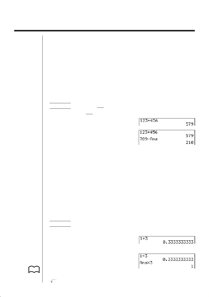
49
2-2 Special Functions
kk
kk
k Answer Function
The unit’s Answer Function automatically stores the last result you calculated by
pressing w(unless the wkey operation results in an error). The result is stored in
the answer memory.
uu
uu
uTo recall the contents of the answer memory
!Kw
uu
uu
uTo use the contents of the answer memory in a calculation
Example 123 + 456 = 579
789 – 579 = 210
Abcd+efgw
hij-!Kw
• The largest value that the answer memory can hold is one with 15 digits for the
mantissa and 2 digits for the exponent.
• Answer memory contents are not cleared when you press the A key or when
you switch power off.
• Note that answer memory contents are not changed by an operation that assigns
values to value memory (such as: faaAw).
kk
kk
k Performing Continuous Calculations
The unit lets you use the result of one calculation as one of the arguments in the next
calculation. To do so, use the result of the previous calculation, which is currently
stored in Answer Memory.
Example 1 ÷ 3 =
1 ÷ 3 × 3 =
Ab/dw
(Continuing)
*dw
Continuous calculations can also be used with Type A functions (x
2
, x
-1
, x!), +, –, ^(x
y
),
x
,
° ’ ”
.
P.19

50
kk
kk
k Using the Replay Function
The Replay Function automatically stores the last calculation performed into replay
memory. You can recall the contents of the replay memory by pressing d or e.
If you press e, the calculation appears with the cursor at the beginning. Pressing
d causes the calculation to appear with the cursor at the end. You can make changes
in the calculation as you wish and then execute it again.
Example To perform the following two calculations
4.12 × 6.4 = 26.368
4.12 × 7.1 = 29.252
Ae.bc*g.ew
dddd
h.b
w
•A calculation remains stored in replay memory until you perform another calcula-
tion or change modes.
• The contents of the replay memory are not cleared when you press the A key,
so you can recall a calculation and execute it even after performing the all clear
operation. Note, however, that replay memory contents are cleared whenever
you change to another mode or menu.
• After you press A, you can press f or c to recall previous calculations, in
sequence from the newest to the oldest (Multi-Replay Function). Once you recall
a calculation, you can use e and d to move the cursor around the calculation
and make changes in it to create a new calculation. Note, however, that multi-
replay memory contents are cleared whenever you change to another menu.
kk
kk
k Making Corrections in the Original Calculation
Example 14 ÷ 0 × 2.3 entered by mistake for 14 ÷ 10 × 2.3
Abe/a*c.dw
Press d or e.
2 - 2 Special Functions
Cursor is positioned automatically at the
location of the cause of the error.

51
Make necessary changes.
d
52
2-3 Function Calculations
kk
kk
k Function Menus
This calculator includes five function menus that give you access to scientific func-
tions that are not printed on the key panel.
• The contents of the function menu differ according to the mode you entered from
the Main Menu before you pressed the K key. The following examples show
function menus that appear in the RUN or PRGM Mode.
uu
uu
uHyperbolic Calculations (HYP)
K6(g)2(HYP)
1 (sinh) ........ Hyperbolic sine
2 (cosh) ....... Hyperbolic cosine
3 (tanh) ........ Hyperbolic tangent
4 (sinh
-1
) ...... Inverse hyperbolic sine
5 (cosh
-1
) ..... Inverse hyperbolic cosine
6 (tanh
-1
) ...... Inverse hyperbolic tangent
uu
uu
uProbability/Distribution Calculations (PROB)
K6(g)3(PROB)
1 (x!) ............ Input a value and select this item to obtain the factorial of the
value.
2 (nPr) ......... Permutation
3 (nCr) ......... Combination
4 (Ran#) ...... Pseudo random number in the range of 0 to 1 (10 decimal
places).
6 (g) ............ Next menu
6(g)
1 (P () .......... Probability P (t)
2 (Q () .......... Probability Q (t)
3 (R () .......... Probability R (t)
4 (t () ............ Normalized variate t (x) value
6 (g) ............ Previous menu
123456
12345 6
12345 6
P.309

53
uu
uu
uNumeric Calculations (NUM)
K6(g)4(NUM)
1 (Abs) ......... Select this item and input a value to obtain the absolute value
of the value.
2 (Int) ........... Select this item and input a value to extract the integer part of
the value.
3 (Frac) ........ Select this item and input a value to extract the fraction part of
the value.
4 (Rnd) ........ Rounds off the value used for internal calculations to 10 sig-
nificant digits (to match the value in the Answer Memory), or to
the number of decimal places (Fix) and number of significant
digits (Sci) specified by you.
5 (Intg) ......... Select this item and input a value to obtain the largest integer
that is not greater than the value.
uu
uu
uAngle Units, Coordinate Conversion, Sexagesimal Operations (ANGL)
K6(g)5(ANGL)
1 (°) ............. Specifies degrees for a specific input value.
2 (r) .............. Specifies radians for a specific input value.
3 (g) ............. Specifies grads for a specific input value.
4 (° ’ ”) ......... Specifies degrees (hours), minutes, seconds when inputting a
sexagesimal value.
←
5 (° ’ ”) ......... Converts decimal value to sexagesimal value.
6 (g) ............ Next menu
6(g)
1 (Pol() ........ Rectangular-to-polar coordinate conversion
2 (Rec() ....... Polar-to-rectangular coordinate conversion
6 (g) ............ Previous menu
←
• The ° ’ ” menu option appears only when there is a calculation result shown on
the display.
123456
123456
123456
Function Calculations 2 - 3

54
uu
uu
uEngineering Notation Calculations (ESYM)
K6(g)6(g)1(ESYM)
1 (m) ............ milli (10
–3
)
2 (µ) ............. micro (10
–6
)
3 (n) ............. nano (10
–9
)
4 (p) ............. pico (10
–12
)
5 (f) .............. femto (10
–15
)
6 (g) ............ Next menu
6(g)
1 (k) ............. kilo (10
3
)
2 (M) ............ mega (10
6
)
3 (G) ............ giga (10
9
)
4 (T) ............. tera (10
12
)
5 (P) ............ peta (10
15
)
6 (g) ............ Next menu
6(g)
1 (E) ............ exa (10
18
)
2 (ENG) ....... Shifts the decimal place of the displayed value three digits to
the left and decreases its exponent by three. When you are
using engineering notation, the engineering symbol is also
changed accordingly (i.e. m → µ).
←
3 (ENG) ....... Shifts the decimal place of the displayed value three digits to
the right and increases its exponent by three. When you are
using engineering notation, the engineering symbol is also
changed accordingly (i.e. µ → m).
6 (g) ............ Previous menu
←
• The ENG and ENG menu options appear only when there is a calculation result
shown on the display.
123456
123456
123456
2 - 3 Function Calculations

55
kk
kk
k Angle Units
• Once you specify an angle unit, it remains in effect until you specify a different
one. The specification is retained even if you switch power off.
• Be sure to specify “Comp” for Calculation/Binary, Octal, Decimal, Hexadecimal
Setting Mode.
Example Operation Display
To convert 4.25 rad to degrees:
!Zcccc
1(Deg)J4.25K6(g)
5(ANGL)2(r)w 243.5070629
47.3° + 82.5rad = 4774.20181°
47.3+82.52(r)w 4774.20181
kk
kk
k Trigonometric and Inverse Trigonometric Functions
• Be sure to set the angle unit before performing trigonometric function and inverse
trigonometric function calculations.
• Be sure to specify “Comp” for Calculation/Binary, Octal, Decimal, Hexadecimal
Setting Mode.
Example Operation Display
sin 63° = 0.8910065242 !Zcccc
1(Deg)J
s63w 0.8910065242
cos (
π
rad) = 0.5 !Zcccc
3
2(Rad)J
c(!7/d)w 0.5
tan (– 35gra) =
– 0.6128007881 !Zcccc
3(Gra)J
t-35w –0.6128007881
2 • sin 45° × cos 65°
= 0.5976724775 !Zcccc
1(Deg)J
2*s45*c65w*
1
0.5976724775
cosec 30° =
1
= 2 1/s30w 2
sin30°
sin
-1
0.5 = 30°
(x when sinx = 0.5) !S0.5*
2
w
30
*
1
* can be omitted.
*
2
Input of leading zero is not necessary.
P.53
P. 5
Function Calculations 2 - 3
P. 5
π
(90° = ––– radians = 100 grads)
2
P. 6
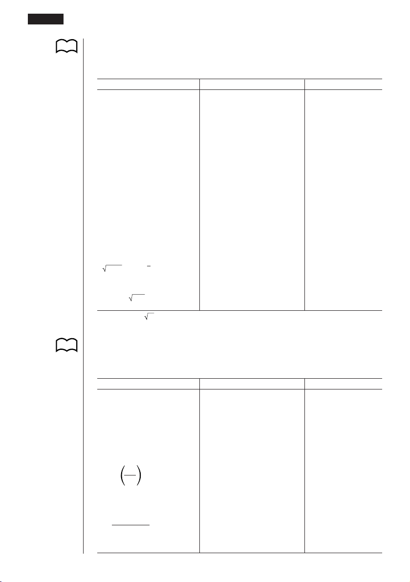
56
kk
kk
k Logarithmic and Exponential Functions
• Be sure to specify “Comp” for Calculation/Binary, Octal, Decimal, Hexadecimal
Setting Mode.
Example Operation Display
log 1.23 (log101.23)
= 8.990511144 × 10
–2
l1.23w 0.08990511144
In 90 (loge90) = 4.49980967 I90w 4.49980967
10
1.23
= 16.98243652
(To obtain the antilogarithm
of common logarithm 1.23) !01.23w 16.98243652
e
4.5
= 90.0171313
(To obtain the antilogarithm
of natural logarithm 4.5) !e4.5w 90.0171313
(–3)
4
= (–3) × (–3) × (–3)
× (–3) = 81 (-3)M4w 81
–3
4
= –(3 × 3 × 3 × 3) = –81 -3M4w – 81
1
7
(= 123
7
)
123
= 1.988647795 7!q123w 1.988647795
2 + 3 ×
3
– 4 = 10 2+3*3!q64-4w*
1
10
64
*
1
^ (x
y
) and
x
take precedence over multiplication and division.
kk
kk
k Hyperbolic and Inverse Hyperbolic Functions
• Be sure to specify “Comp” for Calculation/Binary, Octal, Decimal, Hexadecimal
Setting Mode.
Example Operation Display
sinh 3.6 = 18.28545536 K6(g)2(HYP)
1(sinh)3.6w 18.28545536
cosh 1.5 – sinh 1.5 K6(g)2(HYP)
= 0.2231301601 2(cosh)1.5-1(sinh)1.5w 0.2231301601
= e
–1.5
I!Kw – 1.5
(Proof of cosh x ± sinh x = e
±x
)
cosh
–1
20
= 0.7953654612
K6(g)2(HYP)
15
5(cosh
–1
)(20/15)w 0.7953654612
Determine the value of x
when tanh 4 x = 0.88
x
=
tanh
-1
0.88
K6(g)2(HYP)
4
= 0.3439419141 6(tanh
–1
)0.88/4w 0.3439419141
P. 5
P. 5
2 - 3 Function Calculations

57
kk
kk
k Other Functions
• Be sure to specify “Comp” for Calculation/Binary, Octal, Decimal, Hexadecimal
Setting Mode.
Example Operation Display
+
=
3.65028154 !92+!95w 3.65028154
25
(–3)
2
= (–3) × (–3) = 9 (-3)xw 9
–3
2
= –(3 × 3) = –9 -3xw – 9
(3!X-4!X)
!Xw 12
8! (= 1 × 2 × 3 × .... × 8) 8K6(g)3(PROB)
= 40320 1(x!)w 40320
3
= 42
!#(36*42*49)w
42
36 × 42 × 49
Random number generation K6(g)3(PROB)
(pseudo random number 4(Ran#)w (Ex.) 0.4810497011
between 0 and 1.)
What is the absolute value of
the common logarithm of
3
?
4
|
log
3
|
= 0.1249387366
K6(g)4(NUM)
4
1(Abs)l(3/4)w 0.1249387366
What is the integer part of K6(g)4(NUM)
– 3.5? 2(Int)-3.5w – 3
What is the decimal part of K6(g)4(NUM)
– 3.5? 3(Frac)-3.5w – 0.5
What is the nearest integer K6(g)4(NUM)
not exceeding – 3.5? 5(Intg)-3.5w – 4
P. 5
Function Calculations 2 - 3
1
––––––––––– = 12
11
––– – –––
34

58
kk
kk
k Coordinate Conversion
uu
uu
u Rectangular Coordinates
uu
uu
u Polar Coordinates
• With polar coordinates,
θ
can be calculated and displayed within a range of
–180°<
θ
< 180° (radians and grads have same range).
• Be sure to specify “Comp” for Calculation/Binary, Octal, Decimal, Hexadecimal
Setting Mode.
Example To calculate r and
θ°
when x = 14 and y = 20.7
Operation Display
!Zcccc1(Deg)J
K6(g)5(ANGL)6(g)
1(Pol()14,20.7)w Ans
1
–
24.989
–
→ 24.98979792 (r)
2
–
55.928
–
→ 55.92839019 (
θ
)
Example To calculate x and y when r = 25 and
θ
= 56°
Operation Display
!Zcccc1(Deg)J
K6(g)5(ANGL)6(g)
2(Rec()25,56)w Ans
1
–
13.979
–
→ 13.97982259 (x)
2
–
20.725
–
→ 20.72593931 (y)
kk
kk
k Permutation and Combination
uu
uu
u Permutation
uu
uu
u Combination
• Be sure to specify “Comp” for Calculation/Binary, Octal, Decimal, Hexadecimal
Setting Mode.
P. 5
n! n!
nPr = ––––– nCr = –––––––
(n – r)! r! (n – r)!
P. 5
2 - 3 Function Calculations

59
Example To calculate the possible number of different arrangements
using 4 items selected from among 10 items
Formula Operation Display
10P4 = 5040 10K6(g)3(PROB)
2(nPr)4w 5040
Example To calculate the possible number of different combinations of
4 items that can be selected from among 10 items
Formula Operation Display
10C4 = 210 10K6(g)3(PROB)
3(nCr)4w 210
kk
kk
k Fractions
• Fractional values are displayed with the integer first, followed by the numerator
and then the denominator.
• Be sure to specify “Comp” for Calculation/Binary, Octal, Decimal, Hexadecimal
Setting Mode.
Example Operation Display
2$5+3$1$4w 3{13{20
(Conversion to decimal*
1
)M 3.65
1$2578+1$4572w 6.066202547E–04*
2
(Norm 1 display format)
1$2*
..
..
.5w 0.25*
3
1$(1$3+1$4)w*
4
1{5{7
*
1
Fractions can be converted to decimal values and vice versa.
*
2
When the total number of characters, including integer, numerator, denominator and
deliminater marks exceeds 10, the input fraction is automatically displayed in decimal for-
mat.
*
3
Calculations containing both fractions and decimals are calculated in decimal format.
*
4
You can include fractions within the numerator or denominator of a fraction by putting the
numerator or denominator in parentheses.
P. 5
2113
–– + 3 –– = 3 –––
5420
= 3.65
11
––––– + –––––
2578 4572
= 6.066202547 × 10
–4
1
–– × 0.5 = 0.25
2
15
–––––– = 1––
11 7
–– + ––
34
Function Calculations 2 - 3

60
kk
kk
k Engineering Notation Calculations
Input engineering symbols using the engineering notation menu.
• Be sure to specify “Comp” for Calculation/Binary, Octal, Decimal, Hexadecimal
Setting Mode.
Example Operation Display
!Zccccc
cccc4(Eng)J
999k (kilo) + 25k (kilo) 999K
= 1.024M (mega) 6(g)6(g)1(ESYM)
6(g)1(k)+251(k)w 1.024M
9 ÷ 10 = 0.9 = 900m (milli) 9/10w 900.m
K6(g)6(g)1(ESYM)
6(g)6(g)
←
3(ENG)*
1
0.9
←
3(ENG)*
1
0.0009k
2(ENG)*
2
0.9
2(ENG)*
2
900.m
*
1
Converts the displayed value to the next higher engineering unit, by shifting the decimal
point three places to the right.
*
2
Converts the displayed value to the next lower engineering unit, by shifting the decimal
point three places to the left.
P.16
P. 5
2 - 3 Function Calculations

61
kk
kk
k Logical Operators (AND, OR, NOT)
The logical operator menu lets you select the operator you need.
K6(g)6(g)4(LOGIC)
1 (And) ........ AND (logical multiplication)
2 (Or) ........... OR (logical addition)
3 (Not) ......... NOT (negation)
• Be sure to specify “Comp” for Calculation/Binary, Octal, Decimal, Hexadecimal
Setting Mode.
Example What is the logical product of A and B when A = 3 and B = 2?
A AND B = 1
Operation Display
3aa A w
2aaBw
aAK6(g)6(g)
4(LOGIC)1(And)aBw 1
Example What is the logical sum of A and B when A = 5 and B = 1?
A OR B = 1
Operation Display
5aa A w
1aaBw
aAK6(g)6(g)
4(LOGIC)2(Or)aBw 1
Example Negate A when A = 10.
NOT A = 0
Operation Display
10aaAw
K6(g)6(g)
4(LOGIC)3(Not)aAw 0
P. 5
Function Calculations 2 - 3
123456
62
About Logical Operations
•A logical operation always produces either 0 or 1 as its result.
• The following table shows all of possible results that can be produced by AND
and OR operations.
Value or Expression A Value or Expression B
A AND B A OR B
A G 0B G 011
A G 0 B = 0 0 1
A = 0 B G 001
A = 0 B = 0 0 0
• The following table shows the results produced by the NOT operation.
Value or Expression A NOT A
A G 00
A = 0 1
2 - 3 Function Calculations

Solve, Differential/Quadratic
Differential, Integration,
Maximum/Minimum Value,
and Σ Calculations
3-1 Function Analysis Menu
3-2 Solve Calculations
3-3 Differential Calculations
3-4 Quadratic Differential Calculations
3-5 Integration Calculations
3-6 Maximum/Minimum Value Calculations
3-7 Σ Calculations
Chapter
3

64
3-1 Function Analysis Menu
The following describes the items that are available in the menus you use when
performing Solve, differential/ quadratic differential, integration, maximum/minimum
value, and Σ calculations.
When the option menu is on the display, press 4 (CALC) to display the function
analysis menu.
AK4 (CALC)
1 (Solve) ..... Used in Solve calculations
2 (
d/dx)........ Used in differential calculations
3 (d
2
/dx
2
) ..... Used in quadratic differential calculations
4 (∫
dx).......... Used in integration calculations
6 (g) ........... Previous menu
6 (g)
1 (FMin) ...... Used in minimum calculations
2 (FMax) ..... Used in maximum calculations
3 (Σ() ........... Used in Σ calculations
6 (g) ........... Previous menu
123456
123456

65
3-2 Solve Calculations
To solve calculations, first display the function analysis menu, and then input the
values shown in the formula below to determine root x values in the function f(x).
1(Solve) f(x),n,a,b)
With Solve calculations, the root of a function is determined using Newton’s method.
uu
uu
u Newton’s Method
This method is based on the assumption that f(x) can be approximated by a linear
expression within a very narrow range.
First, a starting value (predicted value)
xo is given. Using this starting value as a
base, approximate value x1 is obtained, and then the left side and right side calcula-
tion results are compared. Next, approximate value x1 is used as the initial value to
calculate the next approximate value x2. This procedure is repeated until the differ-
ence between the left side and right side calculated values is less than some minute
value.
uu
uu
uTo perform solve calculations
Example To calculate the value of root x in the following formula when
the initial estimated value is n = 1, the lower limit is a = 0, and the
upper limit is b = 1:
2
x
2
+ 7x – 9 = 0
Input the function f(x).
AK4(CALC)1(Solve)
cvx+hv-j,
P.64
Initial estimate value Upper limit
Lower limit
1 23456

66
Input initial estimated value
n.
b,
Input lower limit a and upper limit b.
a,b)
w
• In the function
f(x), only X can be used as a variable in expressions. Other vari-
ables (A through Z, r,
θ
) are treated as constants, and the value currently as-
signed to that variable is applied during the calculation.
• Input of the closing parenthesis, lower limit a and upper limit b can be omitted.
• Roots obtained using Solve may include errors.
• Since Solve uses Newton’s method, the following can sometimes occur.
—Certain initial estimated values can make it impossible to obtain roots. In this
case, try inputting another value that you assume to be near the root and per-
form the calculation again.
—The calculator may be unable to obtain a root, even though a root exists.
• Due to certain idiosyncrasies of Newton’s method, roots for the following types
of functions tend to be difficult to calculate.
—Periodic functions (i.e. sin
x = 0)
—Functions whose graph produce sharp slopes (i.e. e
x
= 0,
1
/x = 0)
—Discontinuous functions (i.e.
x = 0)
• Note that you cannot use a Solve, differential, quadratic differential, integration,
maximum/minimum value or Σ calculation expression inside of a Solve calcula-
tion term.
3 - 2 Solve Calculations

67
3-3 Differential Calculations
• To perform differential calculations, first display the function analysis menu, and
then input the values shown in the formula below.
2(d/dx) f(x),a,∆x)
The differentiation for this type of calculation is defined as:
In this definition,
infinitesimal
is replaced by a
sufficiently small
∆x, with the value in
the neighborhood of f ' ( a) calculated as:
In order to provide the best precision possible, this unit employs central difference to
perform differential calculations. The following illustrates central difference.
The slopes of point a and point a + ∆x, and of point a and point a – ∆x in function
y = f(x) are as follows:
In the above, ∆
y/∆x is called the forward difference, while ∇y/∇x is the backward
difference.To calculate derivatives, the unit takes the average between the value of
∆y/∆x and ∇y/∇x, thereby providing higher precision for derivatives.
P.64
Increase/decrease of
x
Point for which you want to determine the derivative
d
d/dx ( f (x), a, ∆x) ⇒ ––– f (a)
dx
f (a + ∆x) – f (a)
f '(a) = lim –––––––––––––
∆x∆x→0
f (a + ∆x) – f (a) ∆y f (a) – f (a – ∆x) ∇y
––––––––––––– = ––– , ––––––––––––– = –––
∆x ∆x ∆x ∇x
f (a + ∆x) – f (a)
f '(a)
–––––––––––––
∆x

68
This average, which is called the
central difference
, is expressed as:
uu
uu
uTo perform a differential calculation
Example To determine the derivative at point x = 3 for the function
y = x
3
+ 4x
2
+ x – 6, when the increase/decrease of x is defined as
∆x = 1E – 5
Input the function
f(x).
AK4(CALC)2(d/dx)
vMd+evx
+v-g,
Input point
x = a for which you want to determine the derivative.
d,
Input ∆
x, which is the increase/decrease of x.
bE-f)
w
• In the function f(x), only X can be used as a variable in expressions. Other vari-
ables (A through Z, r,
θ
) are treated as constants, and the value currently as-
signed to that variable is applied during the calculation.
• Input of ∆
x and the closing parenthesis can be omitted. If you omit ∆x, the calcu-
lator automatically uses a value for ∆x that is appropriate for the derivative value
you are trying to determine.
• Discontinuous points or sections with drastic fluctuation can adversely affect pre-
cision or even cause an error.
1 f (a + ∆x) – f (a) f (a) – f (a – ∆x)
f '(a) = ––
––––––––––––– + –––––––––––––
2∆x ∆x
f (a + ∆x) – f (a – ∆x)
= –––––––––––––––––
2∆x
3 - 3 Differential Calculations

69
kk
kk
k Applications of Differential Calculations
• Differentials can be added, subtracted, multiplied and divided with each other.
Example
• Differential results can be used in addition, subtraction, multiplication, and divi-
sion, and in functions.
Example 2 × f '(a), log ( f '(a))
• Functions can be used in any of the terms (f (x), a, ∆x) of a differential.
Example
• Note that you cannot use a Solve, differential, quadratic differential, integration,
maximum/minimum value or Σ calculation expression inside of a differential cal-
culation term.
• Pressing A during calculation of a differential (while the cursor is not shown
on the display) interrupts the calculation.
• Always perform trigonometric differentials using radians (Rad Mode) as the
angle unit.
dd
––– f (a) = f '(a), ––– g (a) = g'(a)
dx dx
Therefore:
f '(a) + g'(a), f '(a) × g'(a)
d
––– (sin
x + cosx, sin0.5)
dx
Differential Calculations 3 - 3

70
3-4 Quadratic Differential Calculations
After displaying the function analysis menu, you can input quadratic differentials
using either of the two following formats.
3(d
2
/dx
2
) f(x),a,n)
Quadratic differential calculations produce an approximate differential value using
the following second order differential formula, which is based on Newton's polyno-
mial interpretation.
–
f(x – 2h) + 16 f(x – h) – 30 f(x) + 16 f(x + h) – f(x + 2h)
f''(x)
=–––––––––––––––––––––––––––––––––––––––––––––––
12h
2
In this expression, values for “sufficiently small increments of x” are sequentially
calculated using the following formula, with the value of m being substituted as m =
1, 2, 3 and so on.
1
h = ––––
5
m
The calculation is finished when the value of f"(x) based on the value of h calcu-
lated using the last value of m, and the value of f"(x) based on the value of h
calculated using the current value of m are identical before the upper n digit is reached.
• Normally, you should not input a value for n. It is recommended that you only
input a value for n when required for calculation precision.
• Inputting a larger value for
n does not necessarily produce greater precision.
uu
uu
uTo perform a quadratic differential calculation
Example To determine the quadratic differential coefficient at the point
where x = 3 for the function y = x
3
+ 4x
2
+ x – 6
Here we will use a final boundary value of n = 6.
Input the function f(
x).
AK4(CALC)3(d
2
/dx
2
)
vMd+evx+
v-g,
P.64
d
2
d
2
––– ( f (x), a, n) ⇒ ––– f (a)
dx
2
dx
2
Final boundary (
n
= 1 to 15)
Differential coefficient point
123456

71
Input 3 as point
a, which is differential coefficient point.
d,
Input 6 as n, which is final boundary.
g)
w
• In the function
f(x), only X can be used as a variable in expressions. Other vari-
ables (A through Z, r,
θ
) are treated as constants, and the value currently as-
signed to that variable is applied during the calculation.
• Input of the final boundary value n and the closing parenthesis can be omitted.
• Discontinuous points or sections with drastic fluctuation can adversely affect pre-
cision or even cause an error.
kk
kk
k Quadratic Differential Applications
• Arithmetic operations can be performed using two quadratic differentials.
Therefore:
f ''(a) + g''(a), f ''(a) × g''(a)
• The result of a quadratic differential calculation can be used in a subsequent
arithmetic or function calculation.
2 × f ''(a), log ( f ''(a) )
• Functions can be used within the terms (
f(x), a, n) of a quadratic differential
expression.
• Note that you cannot use a Solve, differential, quadratic differential, integration,
maximum/minimum value or Σ calculation expression inside of a quadratic differ-
ential calculation term.
• Use only integers within the range of 1 to 15 for the value of final boundary n.
Use of a value outside this range produces an Ma ERROR.
• You can interrupt an ongoing quadratic differential calculation by pressing the
A key.
• You should always specify radians (Rad) as the unit of angle unit before per-
forming a quadratic differential calculation using trigonometric functions.
d
2
d
2
––– f (a) = f ''(a), ––– g (a) = g''(a)
dx
2
dx
2
d
2
––– (sin x + cos x, sin 0.5)
dx
2
Quadratic Differential Calculations 3 - 4

72
3-5 Integration Calculations
To perform integration calculations, first display the function analysis menu, and then
input the values shown in the formula below.
4(∫dx) f(x) , a , b , n )
∫
( f(x), a, b, n) ⇒
∫
a
b
f(x)dx, N = 2
n
N number of divisions
Integration calculations are performed by applying Simpson’s Rule for the f (x) func-
tion you input. This method requires that the number divisions be defined as N = 2
n
,
where the value of n is an integer in the range of 1 through 9. If you do not specify a
value for n, the calculator automatically assigns a value in accordance with the inte-
gration being performed.
As shown in the illustration above, integration calculations are performed by calcu-
lating integral values from
a through b for the function y = f (x) where a < x < b, and
f (x) > 0*. This in effect calculates the surface area of the shaded area in the illustra-
tion.
* If f (x) < 0 where a < x < b, the surface area calculation produces negative values
(surface area × – 1).
Number of Divisions (value for
n
in N = 2
n
,
n
is an integer from 1 through 9)
End Point
Start Point
Area of
∫
a
b
f(x)dx is calculated
P.64

73
uu
uu
uTo perform an integration calculation
Example To perform the integration calculation for the function
∫
1
5
(2x
2
+ 3x + 4) dx
Input the function
f (x).
AK4(CALC)4(∫dx)cvx
+dv+e,
Input the start point and end point.
b,f,
Input the number of divisions.
g)
w
• In the function f(x), only X can be used as a variable in expressions. Other vari-
ables (A through Z, r,
θ
) are treated as constants, and the value currently as-
signed to that variable is applied during the calculation.
• Input of
n and the closing parenthesis can be omitted. If you omit n, the calculator
automatically selects the most appropriate value.
• Calculation precision is theoretically ±1 at the least significant digit of the dis-
played result.
kk
kk
k Application of Integration Calculation
• Integrals can be used in addition, subtraction, multiplication and division.
Example
∫
a
b
f(x) dx +
∫
c
d
g(x) dx
• Integration results can be used in addition, subtraction, multiplication and divi-
sion, in functions.
Example 2 ×
∫
a
b
f(x) dx, log (
∫
a
b
f(x) dx)
• Functions can be used in any of the terms ( f(x), a, b, n) of an integral.
Example
∫
cos 0.5
(sin x + cos x) dx =
∫
(sin x + cos x, sin 0.5, cos 0.5, 5)
sin 0.5
Integration Calculations 3 - 5

74
• Note that you cannot use a Solve, differential, quadratic differential, integration,
maximum/minimum value or Σ calculation expression inside of an integration cal-
culation term.
• Pressing A during calculation of an integral (while the cursor is not shown on
the display) interrupts the calculation.
• Always perform trigonometric integrations using radians (Rad Mode) as the
angle unit.
• This unit utilizes Simpson’s rule for integration calculation. As the number of
significant digits is increased, more calculation time is required. In some cases,
calculation results may be erroneous even after considerable time is spent per-
forming a calculation. In particular, when significant digits are less than 1, an
ERROR (Ma ERROR) sometimes occurs.
• Integration involving certain types of functions or ranges can result in relatively
large errors being generated in the values produced.
Note the following points to ensure correct integration values.
(1)When cyclical functions for integration values become positive or negative for
different divisions, perform the calculation for single cycles, or divide between
negative and positive, and then add the results together.
∫
a
b
f(x)dx =
∫
a
c
f(x)dx + (–
∫
c
b
f(x)dx)
Positive part (
S
) Negative part (
S
)
(2)When minute fluctuations in integration divisions produce large fluctuations in
integration values, calculate the integration divisions separately (divide the large
fluctuation areas into smaller divisions), and then add the results together.
∫
a
b
f(x)dx =
∫
a
x1
f(x)dx +
∫
x1
x2
f(x)dx +.....+
∫
x4
b
f(x)dx
3 - 5 Integration Calculations
Positive
part (S)
Negative part (S)

75
3-6 Maximum/Minimum Value Calculations
After displaying the function analysis menu, you can input maximum/minimum cal-
culations using the formats below, and solve for the maximum and minimum of a
function within interval a < x < b.
uu
uu
uMinimum Value
6(g)1(FMin) f(x) ,
a , b , n )
uu
uu
uMaximum Value
6(g)2(FMax) f(x), a , b , n )
uu
uu
u To perform maximum/minimum value calculations
Example 1 To determine the minimum value for the interval defined by start
point a = 0 and end point b = 3, with a precision of n = 6 for the
function y = x
2
– 4x + 9
Input f(x).
AK4(CALC)
6(g)1(FMin)
vx-ev+j,
Input the interval
a = 0, b = 3.
a,d,
Input the precision
n = 6.
g)
w
P.64
Precision (
n
= 1 ~ 9)
End point of interval
Start point of interval
Precision (
n
= 1 ~ 9)
End point of interval
Start point of interval
1 23456

76
Example 2 To determine the maximum value for the interval defined by start
point a = 0 and end point b = 3, with a precision of n = 6 for the
function y = –x
2
+ 2x + 2
Input f(x).
AK4(CALC)
6(g)2(FMax)
-vx+cv+c,
Input the interval
a = 0, b = 3.
a,d,
Input the precision n = 6.
g)
w
• In the function f(x), only X can be used as a variable in expressions. Other vari-
ables (A through Z, r,
θ
) are treated as constants, and the value currently as-
signed to that variable is applied during the calculation.
• Input of
n and the closing parenthesis following the precision value can be omit-
ted.
• Discontinuous points or sections with drastic fluctuation can adversely affect pre-
cision or even cause an error.
• Note that you cannot use a Solve, differential, quadratic differential, integration,
maximum/minimum value or Σ calculation expression inside of a maximum/mini-
mum calculation term.
• Inputting a larger value for n increases the precision of the calculation, but it also
increases the amount of time required to perform the calculation.
• The value you input for the end point of the interval (b) must be greater than the
value you input for the start point (a). Otherwise an Ma ERROR is generated.
• You can interrupt an ongoing maximum/minimum calculation by pressing the
A key.
• You can input an integer in the range of 1 to 9 for the value of n. Using any
value outside this range causes an error (Arg ERROR).
1 2 3456
3 - 6 Maximum/Minimum Value Calculations

77
3-7 Σ Calculations
To perform Σ calculations, first display the function analysis menu, and then input the
values shown in the formula below.
6(g)3(Σ() ak , k ,
α
,
β
, n )
Σ calculation is the calculation of the partial sum of sequence {
ak}, using the follow-
ing formula.
kk
kk
k Example Σ Calculation
Example To calculate the following:
Use n = 1 as the distance between partitions.
Input sequence {
ak}
AK4(CALC)6(g)3(Σ()
aKx-daK+f,
Input variable used by sequence {
ak}
aK,
Input the initial term of sequence {
ak} and last term of sequence {ak}.
c,g,
Input n.
b)
Distance between partitions
Last term of sequence {
ak
}
Initial term of sequence {
ak
}
Variable used by sequence {
ak
}
β
Σ
(ak, k,
α
,
β
, n) =
Σ
ak
k = α
β
S = a
α
+ a
α
+1
+........+ a
β
=
Σ
ak
k = α
6
Σ
(k
2
– 3k + 5)
k = 2

78
w
• You can use only one variable in the function for input sequence {
ak}.
• Input integers only for the initial term of sequence {
ak} and last term of sequence
{ak}.
• Input of n and the closing parentheses can be omitted. If you omit n, the calcula-
tor automatically uses n = 1.
kk
kk
k Σ Calculation Applications
uu
uu
uArithmetic operations using Σ calculation expressions
Expressions:
Possible operations: Sn + Tn, Sn – Tn, etc.
uu
uu
uArithmetic and function operations using Σ calculation results
2 × S
n, log (Sn), etc.
uu
uu
uFunction operations using Σ calculation terms (
ak, k)
Σ (sink, k, 1, 5), etc.
• Note that you cannot use a Solve, differential, quadratic differential, integration,
maximum/minimum value or Σ calculation expression inside of a Σ calculation
term.
kk
kk
k Σ Calculation Precautions
• Make sure that the value used as the final term
β
is greater than the value used
as the initial term
α
. Otherwise, an Ma ERROR will occur.
• To interrupt an ongoing Σ calculation (indicated when the cursor is not on the dis-
play), press the A key.
nn
Sn =
Σ
ak, Tn =
Σ
bk
k = 1 k = 1
3 - 7 Σ Calculations

Complex Numbers
This calculator is capable of performing the following operations
using complex numbers.
• Arithmetic operations (addition, subtraction, multiplication, divi-
sion)
• Calculation of the reciprocal, square root, and square of a com-
plex number
• Calculation of the absolute value and argument of a complex
number
• Calculation of conjugate complex numbers
• Extraction of the real number part
• Extraction of the imaginary number part
4-1 Before Beginning a Complex Number Calculation
4-2 Performing Complex Number Calculations
4-3 Complex Number Calculation Precautions
Chapter
4

80
4-1 Before Beginning a Complex Number
Calculation
Before beginning a complex number calculation, press K3 (CPLX) to display
the complex number calculation menu.
K3(CPLX)
1 (i) ............. Input of imaginary unit i
2 (Abs) ........ Calculation of absolute value
3 (Arg)......... Calculation of argument
4 (Conj) ....... Calculation of conjugate
5 (ReP) ....... Extraction of real number part
6 (ImP) ........ Extraction of imaginary number part
123456

81
4-2 Performing Complex Number Calculations
The following examples show how to perform each of the complex number calcula-
tions available with this calculator.
kk
kk
k Arithmetic Operations
Arithmetic operations are the same as those you use for manual calculations. You
can even use parentheses and memory.
Example 1 (1 + 2i) + (2 + 3i)
AK3(CPLX)
(b+c1(
i))+
(c+d1(i))w
Example 2 (2 + i) × (2 – i)
AK3(CPLX)
(c+1(
i))*
(c-1(i))w
kk
kk
k Reciprocals, Square Roots, and Squares
Example
(3 + i)
AK3(CPLX)
!9(d+1(
i))w
1 23456
123456
123456

82
kk
kk
k Absolute Value and Argument
The unit regards a complex number in the format Z = a + bi as a coordinate on a
Gaussian plane, and calculates absolute value Z and argument (arg).
Example To calculate absolute value (r) and argument (
θ
) for the complex
number 3 + 4i, with the angle unit set for degrees
AK3(CPLX)2(Abs)
(d+e1(i))w
(Calculation of absolute value)
AK3(CPLX)3(Arg)
(d+e1(
i))w
(Calculation of argument)
• The result of the argument calculation differs in accordance with the current an-
gle unit setting (degrees, radians, grads).
kk
kk
k Conjugate Complex Numbers
A complex number of the format a + bi becomes a conjugate complex number of the
format a – bi.
Example To calculate the conjugate complex number for the complex
number 2 + 4i
AK3(CPLX)4(Conj)
(c+e1(i))w
Imaginary Number Axis
Real Number Axis
4 - 2 Performing Complex Number Calculations
123456
123456
123456

83
kk
kk
k Extraction of Real and Imaginary Number Parts
Use the following procedure to extract real part a and imaginary part b from a com-
plex number with the format a + bi.
Example To extract the real and imaginary parts of the complex number
2 + 5i
AK3(CPLX)5(ReP)
(c+f1(i))w
(Real part extraction)
AK3(CPLX)6(ImP)
(c+f1(
i))w
(Imaginary part extraction)
Performing Complex Number Calculations 4 - 2
1 23456
123456

84
4-3 Complex Number Calculation Precautions
• The input/output range of complex numbers is normally 10 digits for the mantissa
and two digits for the exponent.
• When a complex number has more than 21 digits, the real number part and im-
aginary number part are displayed on separate lines.
• When either the real number part or imaginary number part equals zero, that part
is not displayed.
• 20 bytes of memory are used whenever you assign a complex number to a vari-
able.
• The following functions can be used with complex numbers.
, x
2
, x
–1
← ←
Int, Frac, Rnd, Intg, Fix, Sci, ENG,ENG,° ’ ”,° ’ ”, a
b
/c, d/c, F
⇔
D
P.25

Binary, Octal, Decimal, and
Hexadecimal Calculations
This calculator is capable of performing the following operations
involving different number systems.
•Number system conversion
•Arithmetic operations
•Negative values
•Logical operations
5-1 Before Beginning a Binary, Octal, Decimal, or
Hexadecimal Calculation
5-2 Selecting a Number System
5-3 Arithmetic Operations
5-4 Negative Values and Logical Operations
Chapter
5

86
5-1 Before Beginning a Binary, Octal, Decimal, or
Hexadecimal Calculation
You can use the RUN Mode and binary, octal, decimal, and hexadecimal settings to
perform calculations that involve binary, octal, decimal and hexadecimal values. You
can also convert between number systems and perform logical operations.
• You cannot use scientific functions in binary, octal, decimal, and hexadecimal
calculations.
• You can use only integers in binary, octal, decimal, and hexadecimal calcula-
tions, so fractional values are not allowed. If you input a value that includes a
decimal part, the unit automatically cuts off the decimal part.
• If you attempt to enter a value that is invalid in the number system (binary, octal,
decimal, hexadecimal) you are using, the calculator displays an error message.
The following shows the numerals that can be used in each number system.
Binary: 0, 1
Octal: 0, 1, 2, 3, 4, 5, 6, 7
Decimal: 0, 1, 2, 3, 4, 5, 6, 7, 8, 9
Hexadecimal: 0, 1, 2, 3, 4, 5, 6, 7, 8, 9, A, B, C, D, E, F
• The alphabetic characters used in the hexadecimal number appear differently on
the display to distinguish them from text characters.
Normal Text: A, B, C, D, E, F
Hexadecimal Values: u, v, w , x, y , z
• Negative binary, octal, and hexadecimal values are produced using the two’s
complement of the original value.
• The following are the display capacities for each of the number systems.
Number System Display Capacity
Binary 16 digits
Octal 11 digits
Decimal 10 digits
Hexadecimal 8 digits
• The following are the calculation ranges for each of the number systems.
Binary Values
Positive: 0 <
x < 111111111111111
Negative: 1000000000000000 < x < 1111111111111111
P.5

87
Octal Values
Positive: 0 <
x < 17777777777
Negative: 20000000000 < x < 37777777777
Decimal Values
Positive: 0 <
x < 2147483647
Negative: –2147483648 < x < –1
Hexadecimal Values
Positive: 0 <
x < 7FFFFFFF
Negative: 80000000 < x < FFFFFFFF
uu
uu
uTo perform a binary, octal, decimal, or hexadecimal calculation
1. In the main menu, select RUN icon.
2. Press !Z and then specify the defalut number system by pressing 2 (Dec),
3 (Hex), 4 (Bin), or 5 (Oct).
2(Dec)
3. Press J to change to the screen for calculation input.
J
1 (d~o) ........ Number system specification menu
2 (LOG)....... Logical operation menu
Before Beginning a Binary, Octal, Decimal, or Hexadecimal Calculation 5 - 1
1 23456
123456

88
5-2 Selecting a Number System
You can specify decimal, hexadecimal, binary, or octal as the default number system
using the set up screen. After you press the function key that corresponds to the
system you want to use, press w.
uu
uu
uTo convert a displayed value from one number system to another
Example To convert 2210 (default number system) to its binary or octal
value
A!Z2(Dec)J1(d~o)1(d)
ccw
!Z4(Bin)Jw
!Z5(Oct)Jw
uu
uu
uTo specify a number system for an input value
You can specify a number system for each individual value you input. While binary,
octal, decimal, or hexadecimal is set as the default number system, press 1 (d~o)
to display a menu of number system symbols. Press the function key that corre-
sponds to the symbol you want to select and then input the value you want.
1(d ~ o)
1 (d) ............ Specifies decimal for input
value
2 (h) ............ Specifies hexadecimal for
input value
3 (b) ............ Specifies binary for input value
4 (o) ............ Specifies octal for input value
uu
uu
uTo input values of mixed number systems
Example To input 12310 or 10102, when the default number system is
hexadecimal
!Z3(Hex)J
A1(d~o)1(d)bcdw
3(b)babaw
123456

89
5-3 Arithmetic Operations
Example 1 To calculate 101112 + 110102
!Z4(Bin)J
Ababbb+
bbabaw
Example 2 To input and execute 1238 × ABC16, when the default number
system is decimal or hexadecimal
!Z2(Dec)J
A1(d~o)4(o)bcd*
2(h)ABCw
!Z3(Hex)Jw

90
5-4 Negative Values and Logical Operations
While binary, octal, decimal, or hexadecimal is set as the default number system,
press 2 (LOG) to display a menu of negation and logical operators.
2(LOG)
1 (Neg)........ negation
2 (Not)......... NOT
3 (and) ........ AND
4 (or) ........... OR
5 (xor) ......... XOR
6 (xnor) ....... XNOR
kk
kk
k Negative Values
Example To calculate the negative of 1100102
!Z4(Bin)J
A2(LOG)1(Neg)
bbaabaw
kk
kk
k Logical Operations
Example 1 To input and execute “12016 and AD16”
!Z3(Hex)J
Abca2(LOG)
3(and)ADw
Example 2 To calculate “368 or 11102” to its octal value
!Z5(Oct)J
Adg2(LOG)
4(or)J1(d~o)3(b)
bbbaw
Example 3 To negate 2FFFED16
!Z3(Hex)J
A2(LOG)2(Not)
cFFFEDw
123456

Matrix Calculations
26 matrix memories (Mat A through Mat Z) plus a Matrix Answer
Memory (MatAns), make it possible to perform the following matrix
operations.
• Addition, subtraction, multiplication
• Scalar product calculations
• Determinant calculations
• Matrix transposition
• Matrix inversion
• Matrix squaring
• Raising a matrix to a specific power
• Absolute value, integer part extraction, fractional part extraction,
maximum integer calculations
• Matrix modification using matrix commands
6-1 Before Performing Matrix Calculations
6-2 Matrix Cell Operations
6-3 Modifying Matrices Using Matrix Commands
6-4 Matrix Calculations
6
Chapter

92
2 (row)
×
2 (column) matrix
123456
Not dimension preset
6-1 Before Performing Matrix Calculations
In the Main Menu, select the MAT icon and press w to enter the Matrix Mode and
display its initial screen.
1 (DEL) ....... Delete specific matrix
2 (DEL•A).... Delete all matrices
• The maximum matrix dimension (size) is 255 (rows) × 255 (columns).
kk
kk
k About Matrix Answer Memory (MatAns)
The calculator automatically store matrix calculation results in Matrix Answer Memory.
Note the following points about Matrix Answer Memory.
• Whenever you perform a matrix calculation, the current Matrix Answer Memory
contents are replaced by the new result. The previous contents are deleted and
cannot be recovered.
• Inputting values into a matrix does not affect Matrix Answer Memory contents.
kk
kk
k Creating a Matrix
To create a matrix, you must first define its dimensions (size) in the MATRIX list.
Then you can input values into the matrix.
uu
uu
uTo specify the dimensions of a matrix
Example To create a 2-row × 3-column matrix in the area named Mat B
Highlight Mat B.
c
Specify the number of rows.
cw
Specify the number of columns.
d
w
P.106

93
• All of the cells of a new matrix contain the value 0.
• If “Mem ERROR” remains next to the matrix area name after you input the dimen-
sions, it means there is not enough free memory to create the matrix you want.
uu
uu
uTo input cell values
Example To input the following data into Matrix B :
123
456
Select Mat B.
c
w
bwcwdw
ewfwgw
(Data is input into the highlighted cell.
Each time you press w, the highlight-
ing move to the next cell to the right.)
• Displayed cell values show positive integers up to six digits, and negative inte-
gers up to five digits (one digit used for negative sign). Exponential values are
shown with up to two digits for the exponent. Fractional values are not displayed.
• You can see the entire value assigned to a cell by using the cursor keys to move
the highlighting to the cell whose value you want to view.
• The amount of memory required for a matrix is ten bytes per cell. This means that
a 3 × 3 matrix requires 90 bytes of memory (3 × 3 × 10 = 90).
kk
kk
k Deleting Matrices
You can delete either a specific matrix or all matrices in memory.
uu
uu
uTo delete a specific matrix
1. While the MATRIX list is on the display, use f and c to highlight the matrix
you want to delete.
2. Press 1 (DEL).
1 (DEL)
Highlighted cell (up to six digits
can be displayed)
Value in currently highlighted cell
1 23456
Before Performing Matrix Calculations 6 - 1

94
3. Press 1 (YES) to delete the matrix or 6 (NO) to abort the operation without
deleting anything.
• The indicator “None” replaces the dimensions of the matrix you delete.
uu
uu
uTo delete all matrices
1. While the MATRIX list is on the display, press 2 (DEL•A).
2 (DEL•A)
2. Press 1 (YES) to delete all matrices in memory or 6 (NO) to abort the opera-
tion without deleting anything.
• The indicator “None” is shown for all the matrices.
1 23456
6 - 1 Before Performing Matrix Calculations

95
6-2 Matrix Cell Operations
You can perform any of the following operations involving the cells of a matrix on the
display.
• Row swapping, scalar product, addition
• Row deletion, insertion, addition
• Column deletion, insertion, addition
Use the following procedure to prepare a matrix for cell operations.
1. While the MATRIX list is on the display, use f and c to highlight the name of
the matrix you want to use.
2. Press w.
12
Matrix A =
34
56
1 (R•OP) ..... Row calculation menu
2 (ROW)...... Row operation menu
3 (COL) ....... Column operation menu
All of the following examples use Matrix A recalled by the above operation.
kk
kk
k Row Calculations
The following menu appears whenever you press 1 (R•OP) while a recalled matrix
is on the display.
1(R•OP)
1 (Swap) ..... Row swap
2 (xRw) ....... Scalar product for a specific row
3 (xRw+) ..... Addition of scalar product of specific row to another row
4 (Rw+) ....... Addition of contents of specific row to another row
uu
uu
uTo swap two rows
Example To swap rows two and three of the following matrix :
12
Matrix A =
34
56
123456
123456

96
1(R•OP)1(Swap)
Input the number of the rows you want to swap.
cw
dw
uu
uu
uTo calculate the scalar product of a row
Example To calculate the scalar product of row 2 of the following matrix by 4 :
12
Matrix A =
34
56
1(R•OP)
2(×Rw)
Input multiplier value.
ew
Specify row number.
cw
uu
uu
uTo calculate the scalar product of a row and add the result to
another row
Example To calculate the scalar product of row 2 of the following matrix
by 4 and add the result to row 3 :
12
Matrix A =
34
56
1(R•OP)
3(×Rw+)
Input multiplier value.
ew
Specify number of row whose scalar product
should be calculated.
cw
Specify number of row where result should be
added.
dw
6 - 2 Matrix Cell Operations

97
uu
uu
uTo add two rows together
Example To add row 2 to row 3 of the following matrix :
12
Matrix A =
34
56
1(R•OP)
4(Rw+)
Specify number of row to be added.
cw
Specify number of row to be added to.
dw
kk
kk
k Row Operations
The following menu appears whenever you press 2 (ROW) while a recalled matrix
is on the display.
2 (ROW)
1 (DEL) ....... Delete row
2 (INS) ........ Insert row
3 (ADD)....... Add row
uu
uu
uTo delete a row
Example To delete row 2 of the following matrix :
12
Matrix A =
34
56
2(ROW)c
1(DEL)
123456
123456
Matrix Cell Operations 6 - 2

98
uu
uu
uTo insert a row
Example To insert a new row between rows one and two of the following
matrix :
12
Matrix A =
34
56
2(ROW)c
2(INS)
uu
uu
uTo add a row
Example To add a new row below row 3 of the following matrix :
12
Matrix A =
34
56
2(ROW)cc
3(ADD)
1 2 3456
123456
6 - 2 Matrix Cell Operations

99
kk
kk
k Column Operations
The following menu appears whenever you press 3 (COL) while a recalled matrix
is on the display.
3 (COL)
1 (DEL) ....... Delete column
2 (INS) ........ Insert column
3 (ADD)....... Add column
uu
uu
uTo delete a column
Example To delete column 2 of the following matrix :
12
Matrix A =
34
56
3(COL)e
1(DEL)
uu
uu
uTo insert a column
Example To insert a new column between columns 1 and 2 of the
following matrix :
12
Matrix A =
34
56
3(COL)e
123456
123456
123456
Matrix Cell Operations 6 - 2

100
2(INS)
uu
uu
uTo add a column
Example To add a new column to the right of column 2 of the following
matrix :
12
Matrix A =
34
56
3(COL)e
3(ADD)
123456
6 - 2 Matrix Cell Operations

101
6-3 Modifying Matrices Using Matrix Commands
In addition to using the MATRIX list to create and modify a matrix, you can also use
matrix commands to input data and create a matrix without actually displaying it.
uu
uu
uTo display the matrix commands
1. From the Main Menu, select the RUN icon and press w.
2. Press K to display the option menu.
3. Press 2 (MAT) to display the matrix operation menu.
K2(MAT)
The following describes only the matrix command menu items that are used for
creating matrices and inputting matrix data.
1 (Mat) ........ Mat command (matrix specification)
2 (M→L)...... Mat→List command (assign contents of selected column to
list file)
5 (Aug) ........ Augment command (link two matrices)
6 (g) ........... Next menu
6(g)
1 (Iden) ....... Identity command (identity matrix input)
2 (Dim) ........ Dim command (dimension check)
3 (Fill) .......... Fill command (identical cell values)
6 (g) ........... Previous menu
kk
kk
k Matrix Data Input Format
The following shows the format you should use when inputting data to create a
matrix using the matrix operation menu’s Mat command.
a11 a 12 a1n
a21 a22 a2n
am1 am2 amn
= [ [a11, a12, ..., a1n] [a21, a22, ..., a2n] .... [am1, am2, ..., amn] ]
→ Mat [letter A through Z]
• The maximum value of both m and n is 255.
123456
123456
P.105
P.31

102
Example 1 To input the following data as Matrix A :
135
246
K2(MAT)
![![b,d,f
!]![c,e,g
!]!]a1(Mat)aA
w
• An error (Mem ERROR) occurs if memory becomes full as you are inputting data.
• You can also use the above format inside a program that inputs matrix data.
uu
uu
uTo input an identity matrix
Use the matrix operation menu’s Identity command (1) to create an identity matrix.
Example 2 To create a 3 × 3 identity matrix as Matrix A
K2(MAT)
6(g)1(Iden)da
Number of rows/columns
6(g)1(Mat)aA
w
uu
uu
uTo check the dimensions of a matrix
Use the matrix operation menu’s Dim command (2) to check the dimensions of an
existing matrix.
Example 3 To check the dimensions of Matrix A, which was input in
Example 1
K2(MAT)
6(g)2(Dim)6(g)1(Mat)
a A
1 23456
P.101
1 23456
123456
6 - 3 Modifying Matrices Using Matrix Commands
P.101
Matrix name

103
w
The display shows that Matrix A consists of two rows and three columns.
kk
kk
k Modifying Matrices Using Matrix Commands
You can also use matrix commands to assign values to and recall values from an
existing matrix, to fill in all cells of an existing matrix with the same value, to combine
two matrices into a single matrix, and to assign the contents of a matrix column to a
list file.
uu
uu
uTo assign values to and recall values from an existing matrix
Use the following format with the matrix operation menu’s Mat command (1) to
specify a cell for value assignment and recall.
Mat X [m, n]
X..................... matrix name (A through Z, or Ans)
m.....................row number
n......................column number
Example 1 Assign 10 to the cell at row 1, column 2 of the following matrix :
12
Matrix A =
34
56
baaK2(MAT)1(Mat)
aA![b,c!]
w
Example 2 Multiply the value in the cell at row 2, column 2 of the above
matrix by 5
K2(MAT)1(Mat)
aA![c,c!]
*fw
Modifying Matrices Using Matrix Commands 6 - 3
1 23456
123456
Number of rows
Number of columns
P.101

104
uu
uu
uTo fill a matrix with identical values and to combine two matrices
into a single matrix
Use the matrix operation menu’s Fill command (3) to fill all the cells of an existing
matrix with an identical value and the Augment command (5) to combine two ex-
isting matrices into a single matrix.
Example 1 To fill all of the cells of Matrix A with the value 3
K2(MAT)
6(g)3(Fill)d,
Filler value
6(g)1(Mat)aA
w
Example 2 To combine the following two matrices :
A =
1
B =
3
24
K2(MAT)
5(Aug)1(Mat)aA,
1(Mat)aB
w
• The two matrices you combine must have the same number of rows. An error
(Ma ERROR) occurs if you try to combine two matrices that have different num-
bers of rows.
uu
uu
uTo assign the contents of a matrix column to a list file
Use the following format with the matrix operation menu’s Mat→List command (2)
to specify a column and a list file.
Mat → List (Mat X, m) → List n
X = matrix name (A through Z, or Ans)
m = column number
n = list number
1 23456
123456
6 - 3 Modifying Matrices Using Matrix Commands
P.101
P.101

105
Example To assign the contents of column 2 of the following matrix to list
file 1 :
12
Matrix A = 34
56
K2(MAT)
2(M→L)1(Mat)
aA,c)a
Column number
K1(LIST)1(List)bw
You can use Matrix Answer Memory to assign the results of the above matrix
input and edit operations to a matrix variable. To do so, use the following syntax.
• Fill (n, Mat
α
) → Mat
β
• Augment (Mat
α
, Mat
β
) → Mat
γ
In the above,
α
,
β
, and
γ
are variable names A through Z, and n is any value. The
above does not affect the contents of Matrix Answer Memory.
Modifying Matrices Using Matrix Commands 6 - 3
1 23456

106
6-4 Matrix Calculations
Use the matrix command menu to perform matrix calculation operations.
uu
uu
uTo display the matrix commands
1. From the Main Menu, select the RUN icon and press w.
2. Press K to display the option menu.
3. Press 2 (MAT) to display the matrix command menu.
K2(MAT)
The following describes only the matrix commands that are used for matrix arithme-
tic operations.
1 (Mat) ........ Mat command (matrix specification)
3 (Det)......... Det command (determinant command)
4 (Trn) ......... Trn command (transpose matrix command)
6 (g) ........... Next menu
6 (g)
1 (Iden) ....... Identity command (identity matrix input)
6 (g) ........... Previous menu
All of the following examples assume that matrix data is already stored in memory.
kk
kk
k Matrix Arithmetic Operations
The following is the format for matrix arithmetic operations.
Matrix 1 Arithmetic operator key Matrix 2
Mat A
+
Mat A
- w
Mat Z
*
Mat Z
MatAns MatAns
1 2 3456
123456
P.31

107
Example 1 To add the following two matrices (Matrix A + Matrix B) :
A =
11
B =
23
21 21
1(Mat)aA+
1(Mat)aB
w
This display indicates the following result.
A + B =
34
42
Example 2 To multiply the two matrices in Example 1 (Matrix A × Matrix B)
1(Mat)aA*
1(Mat)aB
w
This display indicates the following result.
A × B =
44
67
• The two matrices must have the same dimensions in order to be added or sub-
tracted. An error (Dim ERROR) occurs if you try to add or subtract matrices of
different dimensions.
• For multiplication, the number of columns in Matrix 1 must match the number of
rows in Matrix 2. Otherwise, an error (Dim ERROR) occurs.
• You can use an identity matrix in place of Matrix 1 or Matrix 2 in the matrix
arithmetic format. Use the matrix command menu’s Identity (1) command to
input the identity matrix.
1 23456
123456
Matrix Calculations 6 - 4

108
Example 3 To multiply Matrix A (from Example 1) by a 2 × 2 identity matrix
1(Mat)aA*
6(g)1(Iden)c
Number of rows and columns.
w
This display indicates the following result.
A × E =
11
21
kk
kk
kMatrix Scalar Product
The following is the format for calculating a matrix scalar product, which multiplies
the value in each cell of the matrix by the same value.
Scalar value Matrix
Mat A
k w
Mat Z
MatAns
Example Calculate the scalar product of the following matrix using a
multiplier value of 4 :
Matrix A =
12
34
e1(Mat)aA
w
This display indicates the following result.
4A =
48
12 16
1 23456
123456
6 - 4 Matrix Calculations

109
kk
kk
k Determinant
The following is the format for obtaining a determinant.
Matrix
Mat A
3 (Det) w
Mat Z
MatAns
Example Obtain the determinant for the following matrix :
123
Matrix A =
456
–1 –2 0
3(Det)1(Mat)aAw
This display indicates determinant |A| = –9.
• Determinants can be obtained only for square matrices (same number of rows
and columns). Trying to obtain a determinant for a matrix that is not square pro-
duces an error (Dim ERROR).
• The determinant of a 2 × 2 matrix is calculated as shown below.
| A | =
a11 a12
= a11 a 22 – a12a21
a21 a22
• The determinant of a 3 × 3 matrix is calculated as shown below.
a11 a12 a13
|A|= a21 a22 a23
a31 a32 a33
= a11 a 22a33 + a12a23a31 + a13a21a32
– a11a23a32 – a12a21a33 – a13a22a31
1 23456
Matrix Calculations 6 - 4

110
kk
kk
k Matrix Transposition
A matrix is transposed when its rows become columns and its columns become
rows. The following is the format for matrix transposition.
Matrix
Mat A
4 (Trn) w
Mat Z
MatAns
Example To transpose the following matrix:
12
Matrix A =
34
56
4(Trn)1(Mat)aA
w
This operation produces the following result.
A
t
=
135
246
kk
kk
kMatrix Inversion
The following is the format for matrix inversion.
Matrix
Mat A
!X w
Mat Z
MatAns
1 23456
6 - 4 Matrix Calculations

111
Example To invert the following matrix :
Matrix A =
12
34
1(Mat)aA!X
w
This operation produces the following result.
A
–1
=
–2 1
1.5 –0.5
• Only square matrices (same number of rows and columns) can be inverted. Try-
ing to invert a matrix that is not square produces an error (Dim ERROR).
• A matrix with a value of zero cannot be inverted. Trying to invert a matrix with
value of zero produces an error (Ma ERROR).
• Calculation precision is affected for matrices whose value is near zero.
• A matrix being inverted must satisfy the conditions shown below.
A A
–1
= A
–1
A = E =
10
01
• The following shows the formula used to invert Matrix A into inverse matrix A
–1
.
A =
ab
cd
A
–1
=
1
d–b
ad – bc
–c a Note that ad – bc
G
0.
kk
kk
k Squaring a Matrix
The following is the format for squaring a matrix.
Matrix
Mat A
xw
Mat Z
MatAns
1 23456
Matrix Calculations 6 - 4

112
Example To square the following matrix :
Matrix A =
12
34
1(Mat)aAx
w
This operation produces the following result.
A
2
=
710
15 22
kk
kk
k Raising a Matrix to a Power
The following is the format for raising a matrix to a power.
Matrix Natural number
Mat A
M k w
Mat Z
MatAns
Example To raise the following matrix to the third power :
Matrix A =
12
34
1(Mat)aAMd
w
This operation produces the following result.
A
3
=
37 54
81 118
1 23456
123456
6 - 4 Matrix Calculations

113
kk
kk
k Determining the Absolute Value, Integer Part, Fraction
Part, and Maximum Integer of a Matrix
The following is the format for using a matrix in built in functions to obtain an abso-
lute value, integer part, fraction part, and maximum integer.
Function command Matrix
Abs Mat A
Frac
w
Int Mat Z
Intg MatAns
Example To determine the absolute value of the following matrix :
Matrix A =
1–2
–3 4
K6(g)4(NUM)1(Abs)
K2(MAT)1(Mat)aA
w
This operation produces the following result.
Abs A =
12
34
• Determinants and inverse matrices are calculated using the elimination method,
so errors (such as dropped digits) may be generated.
• Matrix operations are performed individually on each cell, so calculations may
required considerable time to complete.
• The calculation precision of displayed results for matrix calculations is ± 1 at
the least significant digit.
• If a matrix calculation result is too large to fit into Matrix Answer Memory, an
error (Mem ERROR) occurs.
• You can use the following operations to transfer Matrix Answer Memory con-
tents to another matrix (or when Matrix Answer Memory contains a determinant
to a variable).
MatAns → Mat
α
In the above,
α
is a variable name A through Z. The above does not affect the
contents of Matrix Answer Memory.
1 23456
Matrix Calculations 6 - 4

Equation Calculations
Your graphic calculator can solve the following three types of equa-
tions:
•Linear equations with two to six unknowns
•Quadratic equations
•Cubic equations
7-1 Before Beginning an Equation Calculation
7-2 Linear Equations with Two to Six Unknowns
7-3 Quadratic and Cubic Equations
7-4 What to Do When an Error Occurs
Chapter
7

116
7-1 Before Beginning an Equation Calculations
Before beginning an equation calculation you have to first enter the correct mode,
and you must also clear the equation memories of any data that might be left over
from a previous calculation.
kk
kk
k Entering an Equation Calculation Mode
Highlight the EQUA icon on the Main Menu and then press w.
1(SIML) ....... Linear equation with two to six unknowns
2(POLY) ...... Quadratic or cubic equation
kk
kk
k Clearing Equation Memories
After entering an equation calculation mode (SIML or POLY), clear the calculation
memory for that mode. In the case of SIML, use the function keys to specify the
number of unknowns, from two (1) to six (5). In the case of POLY, use the func-
tion keys to specify either two (1) or three (2) polynomials.
2(DEL)
Press 1 (YES) to clear the equation memories of that mode (SIML or POLY), or
6 (NO) to abort the clear operation without clearing anything.
123456
123456
123456

117
7-2 Linear Equations with Two to Six Unknowns
You can use the procedures described here to solve linear equations with unknowns
that match the following formats:
Two unknowns a1x + b1y = c1
a2x + b2y = c2
Six unknowns a1x + b1y + c1z + d1t + e1u + f1v = g1
a2x + b2y + c2z + d2t + e2u + f2v = g2
a3x + b3y + c3z + d3t + e3u + f3v = g3
a4x + b4y + c4z + d4t + e4u + f4v = g4
a5x + b5y + c5z + d5t + e5u + f5v = g5
a6x + b6y + c6z + d6t + e6u + f6v = g6
• You can also solve linear equations with three, four, and five unknowns. In each
case, the format is similar to those shown above.
kk
kk
k Entering the Linear Equation Mode for Two to Six
Unknowns
While the Equation Mode is displayed, press 1 (SIML).
1(SIML)
1(2) ............. Linear equation with two unknowns
2(3) ............. Linear equation with three unknowns
3(4) ............. Linear equation with four unknowns
4(5) ............. Linear equation with five unknowns
5(6) ............. Linear equation with six unknowns
123456

118
kk
kk
k Solving Linear Equations with Three Unknowns
Example To solve the following linear equations for x, y, and z:
4x + y –2z=–1
x+6y+3z=1
–5x +4y+ z =–7
While in the Linear Equation Mode (SIML), press 2 (3), because the linear equa-
tions being solved have three unknowns.
2(3)
Input each coefficient.
ewbw-cw
-bw
bwgwdwbw
-fwewbw
-hw
Each time you press w, the input value is registered in the highlighted cell. Each
press of w inputs values in the following sequence:
coefficient
a1 → coefficient b1 → coefficient c1 → coefficient d1 →
coefficient
a2 → coefficient b2 → coefficient c2 → coefficient d2 →
coefficient a3 → coefficient b3 → coefficient c3 → coefficient d3
• You can input fractions and value memory contents as coefficients.
After inputting the coefficients, solve the equations.
1(SOLV)
1 23456
123456
7 - 2 Linear Equations with Two to Six Unknowns
Highlighted solution cell value
Value being input into highlighted cell
Coefficient input cells

119
• Internal calculations are performed using a 15-digit mantissa, but results are dis-
played using a 10-digit mantissa and 2-digit exponent.
• This unit performs simultaneous linear equations by placing the coefficients in-
side of a matrix. Because of this, as the coefficient matrix approaches zero, pre-
cision in the inverse matrix is reduced and so precision in the results produced
also deteriorates. For example, the solution for a linear equation with three un-
knowns would be calculated as shown below.
xa1b1c1
–1
d1
y = a2 b2 c2 d2
za3b3c3 d3
• An “Ma ERROR” occurs whenever the unit is unable to solve the equations.
• Pressing 1 (REPT) returns to the initial display of the Linear Equation Mode.
Depending on the coefficients that you use, it may take considerable time for
the calculation result of simultaneous linear equations to appear on the dis-
play. Failure of a result to appear immediately does not mean that the unit is
not functioning properly.
kk
kk
k Changing Coefficients
You can change a coefficient either before or after you register it by pressing w.
uu
uu
uTo change a coefficient before registering it with
ww
ww
w
Press the A key to clear the current value and then input another one.
uu
uu
uTo change a coefficient after registering it with
ww
ww
w
Use the cursor keys to highlight the cell that contains the coefficient that you want to
change. Next, input the value that you want to change to.
kk
kk
k Clearing All the Coefficients
While in the Linear Equation Mode, press the 3 (CLR) function key. This operation
clears all the coefficients to zero.
3(CLR)
123456
Linear Equations with Two to Six Unknowns 7 - 2

120
7-3 Quadratic and Cubic Equations
This calculator can also solve quadratic and cubic equations that match the following
formats (when a
GG
GG
G 0):
• Quadratic: ax
2
+ bx + c = 0
• Cubic:
ax
3
+ bx
2
+ cx + d = 0
kk
kk
k Entering the Quadratic/Cubic Equation Mode
While in the Equation Mode, press 2 (POLY).
2(POLY)
1(2) ............. Quadratic equation
2(3) ............. Cubic equation
kk
kk
k Solving a Quadratic or Cubic Equation
Example To solve the following cubic equation:
x
3
– 2x
2
– x + 2 = 0
Press 2 (3) to enter the Cubic Equation Mode.
2(3)
Input each coefficient.
bw-cw
-bwcw
123456
123456
Value being input into highlighted cell
Cell for input of coefficients

121
• Each time you press w, the input value is registered in the highlighted cell. Each
press of w inputs values in the following sequence:
coefficient
a → coefficient b → coefficient c → coefficient d
Input for coefficient d is required only for cubic equations.
• You can input fractions and value memory contents as coefficients.
After inputting the coefficients, press 1 (SOLV) to solve the equations.
1(SOLV)
• Internal calculations are performed using a 15-digit mantissa, but results are dis-
played using a 10-digit mantissa and 2-digit exponent.
• An “Ma ERROR” occurs whenever the unit is unable to solve the equations.
• Pressing 1 (REPT) returns to the initial display of the Cubic Equation Mode.
kk
kk
k Quadratic equations that produce multiple root (1 or 2)
solutions or imaginary number solutions
The following examples illustrate how multiple-root solutions and imaginary number
solutions are handled.
uu
uu
uTo solve a cubic equation that produces a multiple-value solution
Example To solve the following cubic equation:
x
3
– 4x
2
+ 5x – 2 = 0
bw-ewfw-cw
1(SOLV)
Quadratic and Cubic Equations 7 - 3
Highlighted solution cell value

122
uu
uu
uTo solve a cubic equation that produces an imaginary number
solution
Example To solve the following cubic equation:
x
3
+ x
2
+ x – 3 = 0
bwbwbw-dw
1(SOLV)
It may take considerable time for the calculation result of cubic equations to
appear on the display. Failure of a result to appear immediately does not mean
that the unit is not functioning properly.
kk
kk
k Changing Coefficients
You can change a coefficient either before or after you register it by pressing w.
uu
uu
uTo change a coefficient before registering it with
ww
ww
w
Press the A key to clear the current value and then input another one.
uu
uu
uTo change a coefficient after registering it with
ww
ww
w
Use the cursor keys to highlight the cell that contains the coefficient that you want to
change. Next, input the value that you want to change to.
kk
kk
k Clearing All the Coefficients
While in the Quadratic or Cubic Equation Mode, press the 3 (CLR) function key.
This operation clears all the coefficients to zero.
3(CLR)
7 - 3 Quadratic and Cubic Equations
123456

123
7-4 What to Do When an Error Occurs
uu
uu
uError during coefficient value input
Press the A key to clear the error and return to the value that was registered for the
coefficient before you input the value that generated the error. Try inputting a new
value again.
uu
uu
uError during calculation
Press the A key to clear the error and display coefficient a. Try inputting values for
the coefficients again.
• Note that even when you press the A key, the values assigned for coefficients
are retained.

Graphing
A collection of versatile graphing tools plus a large 127 × 63-dot
display makes it easy to draw a variety of function graphs quickly
and easily. This calculator is capable of drawing the following types
of graphs.
• Rectangular coordinate (Y =) graphs
• Polar coordinate (r =) graphs
• Parametric graphs
• X = constant graphs
• Inequality graphs
• Integration graphs (in the RUN mode only)
A selection of graph commands also makes it possible to incorpo-
rate graphing into programs.
8-1 Before Trying to Draw a Graph
8-2 View Window (V-Window) Settings
8-3 Graph Function Operations
8-4 Graph Memory
8-5 Drawing Graphs Manually
8-6 Other Graphing Functions
8-7 Picture Memory
8-8 Graph Background
Chapter
8

126
8-1 Before Trying to Draw a Graph
kk
kk
k Entering the Graph Mode
On the Main Menu, select the GRAPH icon and enter the GRAPH Mode. When you
do, the Graph Function menu appears on the display. You can use this menu to store,
edit, and recall functions and to draw their graphs.
1 (SEL)........ Draw/non-draw status
2 (DEL) ....... Graph delete
3 (TYPE) ..... Graph Type Menu
5 (GMEM) ... Graph memory save/recall
6 (DRAW).... Draws graph
Memory area
Use
f
and
c
to change selection.
123456

127
8-2 View Window (V-Window) Settings
Use the View Window to specify the range of the x-and y-axes, and to set the spac-
ing between the increments on each axis. You should always set the View Window
parameters you want to use before drawing a graph. Press ! 3 to display the
View Window.
1. Press !3 to display the View Window.
!3(V-Window)
1 (INIT)........ View Window initial settings
2 (TRIG)...... View Window initial settings using specified angle unit
3 (STD) ....... Standardized View Window settings
4 (STO) ....... Store View Window settings to View Window memory.
5 (RCL) ....... Recall View Window settings from View Window memory.
X min .............. Minimum
x-axis value
X max ............. Maximum
x-axis value
X scale ........... Spacing of x-axis increments
Y min .............. Minimum y-axis value
Y max ............. Maximum y-axis value
Y scale ........... Spacing of
y-axis increments
The following illustration shows the meaning of each of these parameters.
123456
P.129
P.129
P.130
P.130
P.130
X min
X scale
Y min
Y max
X max
Y scale
(x, y)

128
2. Input a value for a parameter and press w. The calculator automatically selects
the next parameter for input.
• You can also select a parameter using the c and f keys.
• There are actually nine View Window parameters. The remaining three param-
eters appear on the display when you move the highlighting down past the Y
scale parameter by inputting values and pressing c.
T,
θ
min .......... T,
θ
minimum values
T,
θ
max......... T,
θ
maximum values
T,
θ
pitch ........ T,
θ
pitch
The following illustration shows the meaning of each of these parameters.
3. To exit the View Window, press J or ! Q.
• Pressing w without inputting any value also exits the View Window.
• The following is the input range for View Window parameters.
–9.9999E+97 to 9.99999E+97
• You can input parameter values up to 14 digits long. Values greater than 10
7
or
less than 10
-2
, are automatically converted to a 7-digit mantissa (including nega-
tive sign) plus a 2-digit exponent.
• The only keys that enabled while the View Window is on the display are: a to
j, ., E, -, f, c, d, e, +, -, *, /, (, ), ! 7,
J, ! Q. You can use - or - to input negative values.
• The existing value remains unchanged if you input a value outside the allow-
able range or in the case of illegal input (negative sign only without a value).
• Inputting a View Window range so the min value is greater than the max value,
the axis is inverted.
• You can input expressions (such as 2π) as View Window parameters.
• When the View Window setting does not allow display of the axes, the scale for
the
y-axis is indicated on either the left or right edge of the display, while that for
the x-axis is indicated on either the top or bottom edge.
8 - 2 View Window (V-Window) Settings
(r
,
θ
)
or
(
X, Y
)
min
max
pitch

129
• When View Window values are changed, the graph display is cleared and the
newly set axes only are displayed.
• View Window setting may cause irregular scale spacing.
• Setting maximum and minimum values that create too wide of a View Window
range can result in a graph made up of disconnected lines (because portions of
the graph run off the screen), or in graphs that are inaccurate.
• The point of deflection sometimes exceeds the capabilities of the display with
graphs that change drastically as they approach the point of deflection.
• Setting maximum and minimum values that create to narrow of a View Window
range can result in an error (Ma ERROR).
kk
kk
k Initializing and Standardizing the View Window
uu
uu
u To initialize the View Window
a. Press !3 (V-Window) 1 (INIT) to initialize the View Window to the following
settings.
Xmin = –6.3 Ymin = –3.1
Xmax = 6.3 Ymax = 3.1
Xscale = 1 Yscale = 1
b. Press ! 3 (V-Window) 2 (TRIG) to initialize the View Window to the follow-
ing settings.
Deg Mode
Xmin = –540 Ymin = –1.6
Xmax = 540 Ymax = 1.6
Xscale = 90 Yscale = 0.5
Rad Mode
Xmin = –9.4247779
Xmax = 9.42477796
Xscale = 1.57079632
Gra Mode
Xmin = –600
Xmax = 600
Xscale = 100
• The settings for Y min, Y max, Y pitch, T/
θ
min, T/
θ
max, and T/
θ
pitch remain
unchanged when you press 2 (TRIG).
View Window (V-Window) Settings 8 - 2

130
123456
8 - 2 View Window (V-Window) Settings
uu
uu
u To standardize the View Window
Press !3 (V-Window) 3 (STD) to standardize the View Window to the follow-
ing settings.
Xmin = –10 Ymin = –10
Xmax = 10 Ymax = 10
Xscale = 1 Yscale = 1
kk
kk
k View Window Memory
You can store up to six sets of View Window settings in View Window memory for
recall when you need them.
uu
uu
uTo save View Window settings
Example To save the following View Window settings :
Xmin =–5 Ymin =–5
Xmax = 5 Ymax = 5
Xscale = 1 Yscale = 1
4(STO)
1(V·W1)
• Storing View Window settings in a memory area (V·W1 through V·W6) that al-
ready contains settings replaces the existing settings with the new ones.
uu
uu
uTo recall View Window settings
Example To recall the View Window settings in V·W1
5(RCL)
123456

131
1(V·W1)
• Recalling View Window settings causes the settings currently on the display to be
deleted.
• You can change View Window settings in a program using the following syntax.
View Window [X min value], [X max value], [X scale value],
[Y min value], [Y max value], [Y scale value],
[T,
θ
min value], [T,
θ
max value], [T,
θ
pitch value]
View Window (V-Window) Settings 8 - 2

132
8-3 Graph Function Operations
You can store up to 20 functions in memory. Functions in memory can be edited,
recalled, and graphed. The types of functions that can be stored in memory are:
rectangular coordinate functions, polar coordinate functions, parametric functions,
inequalities, and X = constant expressions.
kk
kk
k Specifying the Graph Type
Before you can store a graph function in memory, you must first specify its graph
type.
1. While the Graph Function Menu is on the display, press 3 (TYPE) to display a
Graph Type Menu.
3(TYPE)
1 (Y =)......... Rectangular coordinate
graph
2 (
r =).......... Polar coordinate graph
3 (Parm)...... Parametric graph
4 (X = c) ...... X = constant graph
6 (g) ........... Next menu
6(g)
1 (Y >)......... Y > f
(x) inequality
2 (Y <)......... Y < f
(x) inequality
3 (Y ≥) ......... Y > f
(x) inequality
4 (Y ≤) ......... Y <
f
(x) inequality
6 (g) ........... Previous menu
2. Press the function key that corresponds to the graph type you want to specify.
kk
kk
k Storing Graph Functions
uu
uu
uTo store a rectangular coordinate function (Y =)
Example To store the following expression in memory area Y1 :
y = 2 x
2
– 5
3(TYPE)1(Y =)
(Specifies rectangular coordinate
expression.)
cvx-f
(Inputs expression.)
123456
123456
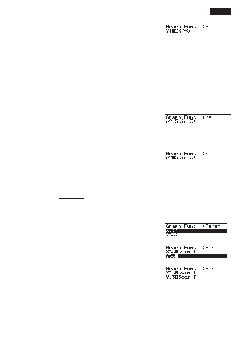
133
w
(Stores expression.)
• You will not be able to store the expression in an area that already contains a
parametric function. Select another area to store your expression or delete the
existing parametric function first. This also applies when storing r = expressions,
X = constant expressions, and ineqalities.
uu
uu
uTo store a polar coordinate function (r =)
Example To store the following expression in memory area r2 :
r = 5 sin 3
θ
3(TYPE)2(r =)
(Specifies polar coordinate expression.)
fsdv
(Inputs expression.)
w
(Stores expression.)
uu
uu
uTo store a parametric function
Example To store the following functions in memory areas Xt3 and Yt3 :
x = 3 sin T
y = 3 cos T
3(TYPE)3(Parm)
(Specifies parametric expression.)
dsvw
(Inputs and stores x expression.)
dcvw
(Inputs and stores y expression.)
• You will not be able to store the expression in an area that already contains a
rectangular coordinate expression, polar coordinate expression, X = constant
expression or inequality. Select another area to store your expression or delete
the existing expression first.
Graph Function Operations 8 - 3

134
8 - 3 Graph Function Operations
uu
uu
uTo store an X = constant expression
Example To store the following expression in memory area X4 :
X = 3
3(TYPE)4(X = c)
(Specifies X = constant expression.)
d
(Inputs expression.)
w
(Stores expression.)
• Inputting X, Y, T, r, or
θ
for the constant in the above procedures causes an error
(Syn ERROR).
uu
uu
uTo store an inequality
Example To store the following inequality in memory area Y5 :
y > x
2
– 2x – 6
3(TYPE)6(g)1(Y>)
(Specifies an inequality.)
vx-cv-g
(Inputs expression.)
w
(Stores expression.)
kk
kk
k Editing Functions in Memory
uu
uu
uTo edit a function in memory
Example To change the expression in memory area Y1 from y = 2x
2
– 5
to y = 2x
2
– 3
e
(Displays cursor.)
eeeed
(Changes contents.)
w
(Stores new graph function.)

135
uu
uu
uTo delete a function
1. While the Graph Function Menu is on the display, press f or c to display the
cursor and move the highlighting to the area that contains the function you want
to delete.
2. Press 2 (DEL).
3. Press 1 (YES) to delete the function for 6 (NO) to abort the procedure with-
out deleting anything.
Parametric functions come in pairs (Xt and Yt).
When editing a parametric function, clear the graph functions and re-input from the
beginning.
kk
kk
k Drawing a Graph
Before actually drawing a graph, you should first make the following specification.
uu
uu
uTo specify the draw/non-draw status of a graph
You can specify which functions out of those stored in memory should be used for a
draw operation.
• Graphs for which there is no draw/non-draw status specification are not drawn.
Example To select the following functions for drawing :
Y1 = 2x
2
– 5
r2 = 5 sin3
θ
Use the following View Window parameters.
Xmin =–5 Ymin =–5
Xmax = 5 Ymax = 5
Xscale = 1 Yscale = 1
cc
(Select a memory area that contains a
function for which you want to specify
non-draw.)
1(SEL)
(Specify non-draw.)
1 23456
Graph Function Operations 8 - 3
1 23456
Unhighlights

136
cc1(SEL)
c1(SEL)
6(DRAW) or w
(Draws graphs.)
• Pressing ! 6 (G↔T) or A returns to the Graph Function Menu.
• You can use the set up screen settings to alter the appearance of the graph
screen as shown below.
• Grid: On
This setting causes dots to appear at the grid intersects on the display.
• Axes: Off
This setting clears the axis lines from the display.
• Label: On
This setting displays labels for the x- and y-axes.
8 - 3 Graph Function Operations
123456
P.6

137
• A polar coordinate (r =) or parametric graph will appear coarse if the settings
you make in the View Window cause the T,
θ
pitch value to be too large, relative
to the differential between the T,
θ
min and T,
θ
max settings. If the settings you
make cause the T,
θ
pitch value to be too small relative to the differential be-
tween the T,
θ
min and T,
θ
max settings, on the other hand, the graph will take
a very long time to draw.
• Attempting to draw a graph for an expression in which X is input for an X =
constant expression results in an error (Syn ERROR).
Graph Function Operations 8 - 3

138
8-4 Graph Memory
Graph memory lets you store up to six sets of graph function data and recall it later
when you need it.
A single save operation saves the following data stored in graph memory.
• All graph functions in the currently displayed Graph Function Menu (up to 20)
• Graph types
• Draw/non-draw status
• View Window settings (1 set)
uu
uu
uTo save graph functions in graph memory
Example To store the graph functions shown on the screen below in graph
memory GM1
5(GMEM)
1(STO)
1(GM1)
• Storing data in a memory area (GM1 through GM6) that already contains data
replaces the existing data with the new data.
• If the data exceeds the calculator’s remaining memory capacity, an error (Mem
ERROR) occurs.
123456
123456
123456

139
uu
uu
uTo recall graph functions from graph memory
Example To recall the data in graph memory GM1
5(GMEM)
2(RCL)
1(GM1)
• Recalling data from graph memory causes any data currently on the Graph Func-
tion Menu to be deleted.
123456
123456
123456
Graph Memory 8 - 4

140
8-5 Drawing Graphs Manually
After you select the RUN icon in the Main Menu and enter the RUN Mode, you can
draw graphs manually. First press ! 4 (Sketch) 5 (GRPH) to recall the Graph
Command Menu, and then input the graph function.
!4(Sketch)
5(GRPH)
1 (Y =)......... Rectangular coordinate graph
2 (r =).......... Polar coordinate graph
3 (Parm)...... Parametric graph
4 (X = c) ...... X = constant graph
5 (G∫
dx) ....... For drawing integration graphs
6 (g) ........... Next menu
6(g)
1 (Y >)......... Y > f
(x) inequality
2 (Y <)......... Y < f
(x) inequality
3 (Y ≥) ......... Y >
f
(x) inequality
4 (Y ≤) ......... Y < f
(x) inequality
6 (g) ........... Previous menu
uu
uu
uTo graph using rectangular coordinates (Y =)
You can graph functions that can be expressed in the format y = f(x).
Example To graph y = 2x
2
+ 3x – 4
Use the following View Window parameters.
Xmin =–5 Ymin =–10
Xmax = 5 Ymax = 10
Xscale = 2 Yscale = 5
1. In the set-up screen, specify the appropriate graph type for Func Type.
!Zc1(Y =)J
2. Input the rectangular coordinate (Y =) expression.
!4(Sketch)1(Cls)w
5(GRPH)1(Y =)
cvx+dv-e
123456
123456

141
3. Press w to draw the graph.
w
• You can draw graphs of the following built-in scientific functions.
• sin x • cos x • tan x
• sin
–1
x • cos
–1
x • tan
–1
x
• sinh x • cosh x • tanh x
• sinh
–1
x • cosh
–1
x • tanh
–1
x
• • x
2
• log x
• lnx • 10
x
• e
x
• x
–1
•
3
View Window settings are made automatically for built-in graphs.
uu
uu
uTo graph using polar coordinates (r =)
You can graph functions that can be expressed in the format r = f
(
θ
).
Example To graph r = 2 sin3
θ
Use the following View Window parameters.
Xmin = –3 Ymin = –2
Xmax = 3 Ymax = 2
Xscale = 1 Yscale = 1
T,
θ
min = 0 T,
θ
max = π
T,
θ
pitch = π÷36
1. In the set-up screen, specify the appropriate graph type for Func Type.
!Zc2(
r =)
2. Set the default unit of angular measurement to radians (Rad).
ccc2(Rad)J
Drawing Graphs Manually 8 - 5

142
3. Input the polar coordinate expression (
r =).
!4(Sketch)1(Cls)w
5(GRPH)2(r =)
csdv
4. Press w to draw the graph.
w
• You can draw graphs of the following built-in scientific functions.
• sin
θ
• cos
θ
• tan
θ
• sin
–1
θ
• cos
–1
θ
• tan
–1
θ
• sinh
θ
• cosh
θ
• tanh
θ
• sinh
–1
θ
• cosh
–1
θ
• tanh
–1
θ
•
θ
•
θ
2
• log
θ
• ln
θ
• 10
θ
• e
θ
•
θ
–1
•
3
θ
• View Window settings are made automatically for built-in graphs.
uu
uu
uTo graph parametric functions
You can graph parametric functions that can be expressed in the following format.
(X, Y) = (f (T), g(T))
Example To graph the following parametric functions:
x = 7 cos T – 2 cos 3.5T
y = 7 sin T – 2 sin 3.5T
Use the following View Window parameters.
Xmin = –20 Ymin = –12
Xmax = 20 Ymax = 12
Xscale = 5 Yscale = 5
T,
θ
min = 0 T,
θ
max = 4π
T,
θ
pitch = π÷36
8 - 5 Drawing Graphs Manually

143
1. In the set-up screen, specify the appropriate graph type for Func Type.
!Zc3(Parm)
2. Set the default angle unit to radians (Rad).
ccc2(Rad)J
3. Input the parametric functions.
!4(Sketch)1(Cls)w
5(GRPH)3(Parm)
hcv-ccd.fv,
hsv-csd.fv)
4. Press w to draw the graph.
w
uu
uu
uTo graph X = constant
You can graph functions that can be expressed in the format X = constant.
Example To graph X = 3
Use the following View Window parameters.
Xmin =–5 Ymin =–5
Xmax = 5 Ymax = 5
Xscale = 1 Yscale = 1
1. In the set-up screen, specify the appropriate graph type for Func Type.
!Zc4(X = c)J
2. Input the expression.
!4(Sketch)1(Cls)w
5(GRPH)4(X = c)d
Drawing Graphs Manually 8 - 5
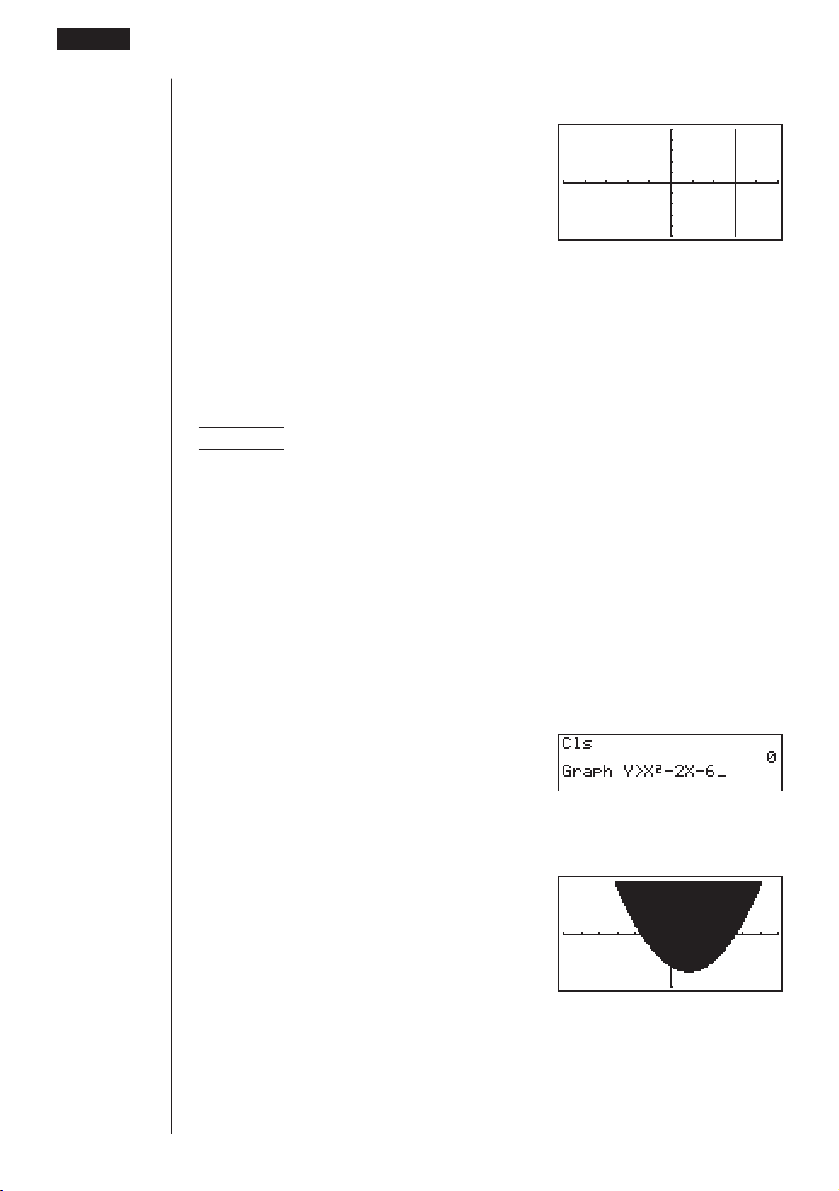
144
3. Press w to draw the graph.
w
uu
uu
uTo graph inequalities
You can graph inequalities that can be expressed in the following four formats.
• y > f
(x)
• y < f
(x)
•
y > f
(x)
• y < f
(x)
Example To graph the inequality y > x
2
– 2x – 6
Use the following View Window parameters.
Xmin =–6 Ymin =–10
Xmax = 6 Ymax = 10
Xscale = 1 Yscale = 5
1. In the set-up screen, specify the appropriate graph type for Func Type.
!Zc6(g)1(Y>)J
2. Input the inequality.
!4(Sketch)1(Cls)w
5(GRPH)6(g)
1(Y>)vx-cv-g
3. Press w to draw the graph.
w
8 - 5 Drawing Graphs Manually

145
uu
uu
uTo draw an integration graph
You can graph an integration calculation performed using the function y = f(x).
Example To graph the following:
∫
–2
1
(x + 2) (x – 1) (x – 3) dx
Use the following View Window parameters.
Xmin =–4 Ymin =–8
Xmax = 4 Ymax = 12
Xscale = 1 Yscale = 5
1. In the set-up screen, specify the appropriate graph type for Func Type.
!Zc1(Y =)J
2. Input the integration graph expression.
!4(Sketch)1(Cls)w
5(GRPH)5(G∫dx)(v+c)
(v-b)(v-d)
,-c,b,f
3. Press w to draw the graph.
w
• Before drawing an integration graph, be sure to always press ! 4 (Sketch)
1 (Cls) to clear the screen.
• You can also incorporate an integration graph command into programs.
Drawing Graphs Manually 8 - 5

146
8-6 Other Graphing Functions
The functions described in this section tell you how to read the x- and y-coordinates
at a given point, and how to zoom in and zoom out on a graph.
• These functions can be used with rectangular coordinate, polar coordinate, para-
metric, X = constant, and inequality graphs only.
kk
kk
k Connect Type and Plot Type Graphs (Draw Type)
You can use the Draw Type setting of the set-up screen to specify one of two graph
types.
• Connect
Points are plotted and connected by lines to create a curve.
• Plot
Points are plotted without being connected.
kk
kk
k Trace
With trace, you can move a flashing pointer along a graph with the f, c, d, and
e cursor keys and obtain readouts of coordinates at each point. The following
shows the different types of coordinate readouts produced by trace.
• Rectangular Coordinate Graph • Polar Coordinate Graph
• Parametric Function Graph • X = Constant Graph
• Inequality Graph
uu
uu
uTo use trace to read coordinates
Example To determine the points of intersection for graphs produced by
the following functions:
Y1 = x
2
– 3
Y2 = –x + 2
Use the following View Window parameters.
Xmin =–5 Ymin =–10
Xmax = 5 Ymax = 10
Xscale = 1 Yscale = 2
P.6

147
1. After drawing the graphs, press 1 (Trace) to make the pointer appear at the far
left of the graph.
1(Trace)
• The pointer may not be visible on the graph when you press 1 (Trace).
2. Use e to move the pointer to the first intersection.
e
~ e
• Pressing d and e moves the pointer along the graph. Holding down either
key moves the pointer at high speed.
3. Use f and c to move the pointer between the two graphs.
4. Use e to move the pointer to the other intersection.
e
~ e
• To abort a trace operation, press 1 (Trace).
• Do not press the A key while performing a trace operation.
uu
uu
uTo display the derivative
If the Derivative item in the set-up screen is set to “On”, the derivative appears on
the display along with the coordinate values.
Other Graphing Functions 8 - 6
x/y
coordinate values
P.6

148
• The following shows how the display of coordinates and the derivative changes
according to the Graph Type setting.
• Rectangular Coordinate Graph • Polar Coordinate Graph
• Parametric Function Graph • X = Constant Graph
• Inequality Graph
• The derivative is not displayed when you use trace with a built-in scientific func-
tion.
• Setting the Coord item in the set-up screen to “Off” turns display of the coordi-
nates for the current pointer location off.
uu
uu
uScrolling
When the graph you are tracing runs off the display along either the x- or y-axis,
pressing the e or d cursor key causes the screen to scroll in the corresponding
direction eight dots.
• You can scroll only rectangular coordinate and inequality graphs while tracing.
You cannot scroll polar coordinate graphs, parametric function graphs, or X =
constant graphs.
• The graph on the screen does not scroll when you are tracing while the Dual
Screen Mode is set to “Graph” or “G to T”.
• Trace can be used only immediately after a graph is drawn. It cannot be used
after changing the settings of a graph.
• The x- and y-coordinate values at the bottom of the screen are displayed using
a 12-digit mantissa or a 7-digit mantissa with a 2-digit exponent. The derivative
is displayed using a 6-digit mantissa.
• You cannot incorporate trace into a program.
• You can use trace on a graph that was drawn as the result of an output com-
mand (^), which is indicated by the “-Disp-” indicator on the screen.
P.8
P.141
8 - 6 Other Graphing Functions
P.6

149
kk
kk
k Scroll
You can scroll a graph along its x- or y-axis. Each time you press f, c , d, or
e, the graph scrolls 12 dots in the corresponding direction.
kk
kk
k Graphing in a Specific Range
You can use the following syntax when inputting a graph to specify a start point and
end point.
<function> , ! [ <start point> , <end point> ! ] w
Example To graph y = x
2
+ 3x – 5 within the range of –2
<<
<<
< x
<<
<<
< 4
Use the following View Window parameters.
Xmin =–3 Ymin =–10
Xmax = 5 Ymax = 30
Xscale = 1 Yscale = 5
3(TYPE)1(Y =)
(Specifies graph type.)
vx+dv-f,
![-c,e!]w
(Stores expression.)
6(DRAW) or w
(Draws graph.)
• You can specify a range for rectangular coordinate, polar coordinate, parametric,
and inequality graphs.
kk
kk
k Overwrite
Using the following syntax to input a graph causes multiple versions of the graph to
be drawn using the specified values. All versions of the graph appear on the display
at the same time.
<function with one variable> , ! [ <variable name> ! =
<value> , <value> , .... <value> ! ] w
123456
Other Graphing Functions 8 - 6

150
Example To graph y = Ax
2
– 3, substituting 3, 1, and –1 for the value of A
Use the following View Window parameters.
Xmin =–5 Ymin =–10
Xmax = 5 Ymax = 10
Xscale = 1 Yscale = 2
3(TYPE)1(Y =)
(Specifies graph type.)
aAvx-d,
![aA!=d,
b,-b!]w
(Stores expression.)
6(DRAW)
(Draws graph.)
↓
↓
• The function input using the above syntax can have only one variable.
• You cannot use X, Y, r,
θ
, or T as the variable name.
• You cannot assign a variable to the variable in the function.
• When the set-up screen’s Simul Graph item is set to “On,” the graphs for all the
variables are drawn simultaneously.
• You can use overwrite with rectangular coordinate, polar coordinate, parametric,
and inequality graphs.
P.8
123456
8 - 6 Other Graphing Functions

151
kk
kk
k Zoom
The zoom feature lets you enlarge and reduce a graph on the display.
uu
uu
uBefore using zoom
Immediately after drawing a graph, press 2 (Zoom) to display the Zoom Menu.
2(Zoom)
1 (BOX)....... Graph enlargement using box zoom
2 (FACT) ..... Displays screen for specification of zoom factors
3 (IN)........... Enlarges graph using zoom factors
4 (OUT)....... Reduces graph using zoom factors
5 (AUTO) .... Automatically sizes the graph so it fills the screen along the
y-
axis.
6 (g) ........... Next menu
6(g)
1 (ORIG) ..... Original size
2 (SQR)....... Adjusts ranges so x-range equals y-range.
3 (RND)....... Rounds coordinates at current pointer location.
4 (INTG)...... Converts
x- and y-axis values to integers.
5 (PRE) ....... After a zoom operation, returns View Window parameters to
previous settings.
6 (g) ........... Previous menu
uu
uu
uTo use box zoom
With box zoom, you draw a box on the display to specify a portion of the graph, and
then enlarge the contents of the box.
Example To use box zoom to enlarge a portion of the graph y = (x + 5)
(x + 4) (x + 3)
Use the following View Window parameters.
Xmin =–8 Ymin =–4
Xmax = 8 Ymax = 2
Xscale = 2 Yscale = 1
123456
123456
P.155
P.156
P.157
P.158
Other Graphing Functions 8 - 6
P.155

152
1. After graphing the function, press 2 (Zoom).
2(Zoom)
2. Press 1 (BOX), and then use the cursor keys (d, e , f, c) to move the
pointer to the location of one of the corners of the box you want to draw on the
screen. Press w to specify the location of the corner.
1(BOX)
d ~ dw
3. Use the cursor keys to move the pointer to the location of the corner that is
diagonally across from the first corner.
f ~ f d ~ d
4. Press w to specify the location of the second corner. When you do, the part of
the graph inside the box is immediately enlarged so it fills the entire screen.
w
• To return to the original graph, press 2 (Zoom) 6 (g) 1 (ORIG).
• Nothing happens if you try to locate the second corner at the same location or
directly above the first corner.
• You can use box zoom for any type of graph.
1 23456
8 - 6 Other Graphing Functions

153
uu
uu
uTo use factor zoom
With factor zoom, you can zoom in or zoom out on the display, with the current
pointer location being at the center of the new display.
• Use the cursor keys (d, e, f, c) to move the pointer around the display.
Example Graph the two functions below, and enlarge them five times in
order to determine whether or not they are tangential.
Y1 = (x + 4) (x + 1) (x – 3)
Y2 = 3x + 22
Use the following View Window parameters.
Xmin =–8 Ymin =–30
Xmax = 8 Ymax = 30
Xscale = 5 Yscale = 10
1. After graphing the functions, press 2 (Zoom), and the pointer appears on the
screen.
2(Zoom)
2. Use the cursor keys (d, e , f, c) to move the pointer to the location that
you want to be the center of the new display.
d ~ d f ~ f
3. Press 2 (FACT) to display the factor specification screen, and input the factor
for the x- and y-axes.
2(FACT)
fwfw
1 2 3456
Other Graphing Functions 8 - 6

154
4. Press J to return to the graphs, and then press 3 (IN) to enlarge them.
J
3(IN)
This enlarged screen makes it clear that the graphs of the two expressions are not
tangential.
Note that the above procedure can also be used to reduce the size of a graph (zoom
out). In step 4, press 4 (OUT).
• The above procedure automatically converts the
x-range and y-range View Win-
dow values to 1/5 of their original settings. Pressing 6 (g) 5 (PRE) changes
the values back to their original settings.
• You can repeat the factor zoom procedure more than once to further enlarge or
reduce the graph.
uu
uu
uTo initialize the zoom factor
Press 2 (Zoom) 2 (FACT) 1 (INIT) to initialize the zoom factor to the following
settings.
Xfact = 2 Yfact = 2
• You can use the following syntax to incorporate a factor zoom operation into a
program.
Factor <X factor>, <Y factor>
• You can specify only positive value up to 14 digits long for the zoom factors.
• You can use factor zoom for any type of graph.
kk
kk
k Using the Auto View Window
The auto View Window feature automatically adjusts y-range View Window values
so that the graph fills the screen along the y-axis.
Example To graph y = x
2
– 5 with Xmin = –3 and Xmax = 5, and then use
auto View Window to adjust the y-range values
1. After graphing the function, press 2 (Zoom).
2(Zoom)
123456
8 - 6 Other Graphing Functions

155
2. Press 5 (AUTO).
5(AUTO)
• You can use auto View Window with any type of graph.
• You cannot use auto View Window inside a program.
• You can use auto View Window with a graph produced by a multi-statement
connected by “:”, even if the multi-statement includes non-graph operations.
• When auto View Window is used in a statement that uses a display result com-
mand (^) to draw a graph, auto View Window parameters are applied up to
the display result command, but any graphs drawn after the display result com-
mand are drawn according to normal graph overdraw rules.
kk
kk
k Adjusting the Ranges of a Graph (SQR)
This function makes the View Window x-range value the same as the y-range value.
It is helpful when drawing circular graphs.
Example To graph r = 5sin
θ
and then adjust the graph.
Use the following View Window parameters.
Xmin =–8 Ymin =–1
Xmax = 8 Ymax = 5
Xscale = 1 Yscale = 1
1. After drawing the graph, press 2 (Zoom) 6 (g).
2(Zoom)6(g)
2. Press 2 (SQR) to make the graph a circle.
2(SQR)
1 2 3456
Other Graphing Functions 8 - 6

156
• You can use SQR with any type of graph.
• You cannot use SQR inside a program.
• You can use SQR with a graph produced by a multi-statement connected by “:”,
even if the multi-statement includes non-graph operations.
• When SQR is used in a statement that uses a display result command (^) to
draw a graph, Graph Adjust parameters are applied up to the display result
command, but any graphs drawn after the display result command are drawn
according to normal graph overwrite rules.
kk
kk
k Rounding Coordinates (RND)
This feature rounds the coordinate values at the pointer location to the optimum
number of significant digits. Rounding coordinates is useful when using trace and
plot.
Example To round the coordinates at the points of intersection of the two
graphs drawn on page 146
Use the same View Window parameters as in the example on page
146.
1. After graphing the functions, press 1 (Trace) and move the pointer to the first
intersection.
1(Trace)
e ~ e
2. Press 2 (Zoom) 6 (g).
2(Zoom)6(g)
3. Press 3 (RND) and then 1 (Trace). Use e to move the pointer to the other
intersection. The rounded coordinate values for the pointer position appear on
the screen.
3(RND)
1(Trace)
e ~ e
8 - 6 Other Graphing Functions
123456

157
• You can use RND with any type of graph.
• You cannot use RND inside a program.
• You can use RND with a graph produced by a multi-statement connected by “:”,
even if the multi-statement includes non-graph operations.
• When RND is used in a statement that uses a display result command (^) to
draw a graph, Rounding Coordinate parameters are applied up to the display
result command, but any graphs drawn after the display result command are
drawn according to normal graph overwrite rules.
kk
kk
k Converting x- and y-axis Values to Integers (INTG)
This feature converts View Window values to the following, and redraws the graph
with the current pointer position as the center point.
Xmin = center point –63.5 Ymin = center point –31.5
Xmax = center point +63.5 Ymax = center point +31.5
Xscale = 10 Yscale = 10
Example To graph y = x
2
– 3 and then redraw it using INTG
Use the following View Window parameters.
Xmin =–5 Ymin =–10
Xmax = 5 Ymax = 10
Xscale = 1 Yscale = 2
1. Press 2 (Zoom) 6 (g) after drawing the graph.
2(Zoom)6(g)
2. Press 4 (INTG).
4(INTG)
Other Graphing Functions 8 - 6
123456

158
• You can use INTG with any type of graph.
• You cannot use INTG inside a program.
• You can use INTG with a graph produced by a multi-statement connected by
“:”, even if the multi-statement includes non-graph operations.
• When INTG is used in a statement that uses a display result command (^) to
draw a graph, Integer parameters are applied up to the display result com-
mand, but any graphs drawn after the display result command are drawn ac-
cording to normal graph overwrite rules.
kk
kk
k Returning the View Window to Its Previous Settings
The following operation returns View Window parameters to their original settings
following a zoom operation.
6 (g) 5 (PRE)
• You can use PRE with a graph altered by any type of zoom operation.
8 - 6 Other Graphing Functions

159
8-7 Picture Memory
You can save up to six graphic image in picture memory for later recall. You can
overdraw the graph on the screen with another graph stored in picture memory.
uu
uu
uTo store a graph in picture memory
The following operation stores all points and lines currently on the screen.
Example To store the graph drawn in the example on page 146 into picture
memory Pic1
K
1(PICT)
1(STO)
1(Pic1)
• Storing a graph in a memory area (Pic1 through Pic6) that already contains a
graph replaces the existing graph with a new one.
uu
uu
uTo recall a graph from memory
Example To recall the graph stored in picture memory Pic1
• In the GRAPH Mode:
K1(PICT)2(RCL)
1(Pic1)
1 23456
123456
123456
123456

160
• Dual Graph screens or any other type of graph that uses a split screen cannot be
saved in picture memory.
8 - 7 Picture Memory

161
8-8 Graph Background
You can use the set-up screen to specify the memory contents of any picture memory
area (Pict 1 through Pict 6) as the Background item. When you do, the contents of
the corresponding memory area is used as the background of the graph screen.
• You can use a background in the RUN, STAT, GRAPH, DYNA, TABLE, RECUR,
CONICS Modes.
Example 1 With the circle graph X
2
+ Y
2
= 1 as the background, use
Dynamic Graph to graph Y = X
2
+ A as variable A changes value
from –1 to 1 in increments of 1.
Recall the background graph.
(X
2
+ Y
2
= 1)
Draw the dynamic graph.
(Y = X
2
+ 1)
↓↑
(Y = X
2
)
↓↑
(Y = X
2
– 1)
• See “14. Implicit Function Graphs” for details on drawing a circle graph, and “13.
Dynamic Graph” for details on using the Dynamic Graph feature.
P.7
P.223
P.207

162
Example 2 With a statistical histogram as the background, graph a normal
distribution
Recall the backgound graph.
(Histogram)
Graph the normal distribution.
• See “18. Statistical Graphs and Calculations” for details on drawing a statistical
graphs.
P.283
8 - 8 Graph Background

Graph Solve
You can use any of the following methods to analyze function graphs
and approximate results.
•Root extraction
•Determination of the maximum and minimum
•Determination of the y-intercept
•Determination of the intersection of two graphs
•Determination of the coordinates at any point (y for a given x/x for
a given y)
•Determination of the integral for any range
9-1 Before Using Graph Solve
9-2 Analyzing a Function Graph
9-3 Graph Solve Precautions
Chapter
9

164
9-1 Before Using Graph Solve
After using the GRAPH Mode to draw the graph, press ! 5 (G-Solv) to display
the graph solve menu.
!5(G-Solv)
1 (ROOT) .... Root
2 (MAX)....... Maximum
3 (MIN)........ Minimum
4 (Y-ICPT) ... y-intercept
5 (ISCT) ...... Intersections of two graphs
6 (g) ........... Next menu
6(g)
1 (Y-CAL) .... y-coordinate for a given x-coordinate
2 (X-CAL).... x-coordinate for a given y-coordinate
3 (∫dx).......... Integral for a given range
6 (g) ........... Previous menu
123456
123456

165
9-2 Analyzing a Function Graph
The following two graphs are used for all of the examples in this section, except for
the example for determining the points of intersection for two graphs.
Memory location Y1 = x + 1
Memory location Y2 =
x(x + 2)(x – 2)
Use the View Window to specify the following parameters.
(A)
Xmin = –5 Ymin = –5
(B)
Xmin = –6.3 Ymin = –3.1
Xmax = 5 Ymax = 5 Xmax = 6.3 Ymax = 3.1
Xscale = 1 Yscale = 1 Xscale = 1 Yscale = 1
kk
kk
k Determining Roots
Example To determine the roots for y = x(x + 2)(x – 2)
View Window: (B)
!5(G-Solv)
1(ROOT)
(This puts the unit into standby waiting
for selection of a graph.)
•A “ k ” cursor appears on the graph that has the lowest memory area number.
Specify the graph you want to use.
c
• Use f and c to move the cursor to the
graph whose roots you want to find.
Determine the root.
w
• Roots are found starting from the left.
1 23456

166
Search for the next root to the right.
e
• If there is no root to the right, nothing happens
when you press e.
e
• You can use d to move back to the left.
• If there is only one graph, pressing 1(ROOT) directly displays the root (selec-
tion of the graph is not required).
• Note that the above operation can be performed on rectangular coordinate (Y=)
and inequality graphs only.
kk
kk
k Determining Maximums and Minimums
Example To determine the maximum and minimum for y = x (x + 2) (x – 2)
View Window: (A)
!5(G-Solv)
2(MAX)
(This puts the unit into standby waiting
for selection of a graph.)
Specify the graph and determine the maximum.
cw
9 - 2 Analyzing a Function Graph
1 2 3456

167
!5(G-Solv)
Specify the graph and determine the minimum.
3(MIN) cw
• If there is more than one maximum/minimum, you can use d and e to move
between them.
• If there is only one graph, pressing 2 (MAX) / 3 (MIN) directly displays the
maximum/minimum (selection of the graph is not required).
• Note that the above operation can be performed on rectangular coordinate (Y=)
and inequality graphs only.
kk
kk
k Determining y-intercepts
Example To determine the y-intercept for y = x + 1
View Window: (B)
!5(G-Solv)
4(Y-ICPT)
(This puts the unit into standby waiting
for selection of a graph.)
Determine the
y-intercept.
w
• y-intercepts are the points that the graph intersects the y-axis.
• If there is only one graph, pressing 4 (Y-ICPT) directly displays the
y-intercepts
(selection of the graph is not required).
• Note that the above operation can be performed on rectangular coordinate (Y=)
and inequality graphs only.
123456
Analyzing a Function Graph 9 - 2
123456

168
kk
kk
k Determining Points of Intersection for Two Graphs
Example To draw the following three graphs and then determine the points
of intersection for the Graph A and Graph C.
View Window: (A)
Graph A: y = x + 1
Graph B: y = x (x + 2) (x – 2)
Graph C: y = x
2
!5(G-Solv)
5(ISCT)
(This puts the unit into standby waiting
for selection of a graph.)
Specify Graph A.
w
• Pressing w changes “ k ” into “ ◆ ” for speci-
fication of the first graph.
Specify the second graph (Graph C, here) to determine the points of intersection.
cw
• Use f and c to move “ k ” on the second
graph.
• Intersections are found starting from the left.
e
• The next intersection to the right is found. If
there is no intersection to the right, nothing
happens when you perform this operation.
• You can use d to move back to the left.
• If there are only two graphs, pressing 5 (ISCT) directly displays the intersec-
tions (selection of the graph is not required).
9 - 2 Analyzing a Function Graph
123456

169
• Note that the above operation can be performed on rectangular coordinate (Y=)
and inequality graphs only.
kk
kk
k Determining a Coordinate (x for a given y/y for a given x)
Example To determine the y-coordinate for x = 0.5 and the x-coordinate for
y = 3.2 in the graph y = x (x + 2) (x – 2)
View Window: (B)
!5(G-Solv)6(g)
1(Y-CAL)
Specify a graph.
cw
• At this time, the unit waits for input of an x-
coordinate value.
Input the x-coordinate value.
a.f
Determine the corresponding y-coordinate value.
w
!5(G-Solv)6(g)
1 23456
123456
Analyzing a Function Graph 9 - 2

170
Specify a graph.
2(X-CAL) cw
• At this time, the unit waits for input of a y-coor-
dinate value.
Input the
y-coordinate value.
d.c
Determine the corresponding x-coordinate value.
w
• If there is more than one x-coordinate value for a given y-coordinate value or
more than one y-coordinate value for a given x-coordinate value, use e and d
to move between them.
• The display used for the coordinate values depends on the graph type as shown
below.
• Polar Coordinate Graph
• Parametric Graph
• Inequality Graph
• Note that you can not determine a y-coordinate for a given x-coordinate with a
parametric graph.
• If there is only one graph, pressing 1 (Y-CAL) / 2 (X-CAL) directly displays
the x-coordinate/y-coordinate (selection of the graph is not required).
9 - 2 Analyzing a Function Graph

171
kk
kk
k Determining the Integral for Any Range
Example
∫
–1.5
0
x (x + 2) (x – 2) dx
View Window: (A)
!5(G-Solv)6(g)
3(∫dx)
(Graph selection standby)
Select graph.
cw
• The display is prompting input of the lower limit
of the integration range.
Move the pointer and input the lower limit.
e~ew
Input the upper limit and determine the integral.
e~ew
• The lower limit must be less than the upper limit when specifying the integration
range.
• Note that the above operation can be performed on rectangular coordinate (Y=)
graphs only.
123456
Analyzing a Function Graph 9 - 2

172
9-3 Graph Solve Precautions
• Depending on the View Window parameter settings, there may be some error in
solutions produced by Graph Solve.
• If no solution can be found for any of the above operations, the message “Not
Found” appears on the display.
• The following conditions can interfere with calculation precision and may make it
impossible to obtain a solution.
* When the solution is a point of tangency to the
x-axis.
* When the solution is a point of tangency between two graphs.

Sketch Function
The sketch function lets you draw lines and graphs on an existing
graph.
• Note that Sketch function operation in the STAT, GRAPH, TA-
BLE, RECUR and CONICS Modes is different from Sketch func-
tion operation in the RUN and PRGM Modes.
10-1 Before Using the Sketch Function
10-2 Graphing with the Sketch Function
Chapter
10

174
10-1 Before Using the Sketch Function
Press ! 4 (Sketch) to display the sketch menu.
STAT, GRAPH, TABLE, RECUR, CONICS Mode
!4(Sketch)
1 (Cls) ......... Clears drawn line and point
2 (Tang)....... Tangent
3 (Norm)...... Line normal to a curve
4 (Inv).......... Inverse graph
6 (g) ........... Next menu
• 2 (Tang), 3 (Norm), and 4 (Inv) appear only when you display the sketch
menu while in the GRAPH and TABLE Modes.
6 (g)
1 (PLOT) ..... Plot menu
2 (LINE) ...... Line menu
3 (Crcl) ........ Circle
4 (Vert) ........ Vertical line
5 (Hztl) ........ Horizontal line
6 (g) ........... Next menu
6 (g)
1 (PEN) ....... Freehand drawing
2 (Text) ........ Comment text
6 (g) ........... Previous menu
123456
123456
123456
P.179
P.182
P.184
P.185
P.185
P.185
P.186
P.188
P.176
P.177
P.178

175
RUN, PRGM Mode
!4(Sketch)
5 (GRPH) .... Graph command menu
6 (g)
6 (g)
3 (PIXL)....... Pixel menu
4 (Test)........ Tests pixel on/off status
• Other menu items are identical to those in the STAT, GRAPH, TABLE, RECUR,
CONICS Mode menu.
123456
123456
123456
Before Using the Sketch Function 10 - 1
P.187
P.188

176
10-2 Graphing with the Sketch Function
The sketch function lets you draw lines and plot points on a graph that is already on
the screen.
All the examples in this section that show operations in the STAT, GRAPH, TABLE,
RECUR, and CONICS Modes are based on the assumption that the following func-
tion has already been graphed in the GRAPH Mode.
Memory Area Y1 =
x(x + 2)(x – 2)
The following are the View Window parameters used when drawing the graph.
Xmin = –5 Ymin = –5
Xmax = 5 Ymax = 5
Xscale = 1 Yscale = 1
kk
kk
k Tangent
This function lets you draw a line that is tangent to a graph at any point.
uu
uu
uTo draw a tangent in the GRAPH or TABLE Mode
Example To draw a line that is tangent to point (x = 2, y = 0) of y = x(x + 2)
(x – 2)
1. After graphing the function, display the sketch menu and press 2 (Tang).
!4(Sketch)2(Tang)
2. Use the cursor keys (f , c, d, e ) to move the pointer the position of the
point where you want to draw the line.
e ~ e
3. Press w to draw the line.
w
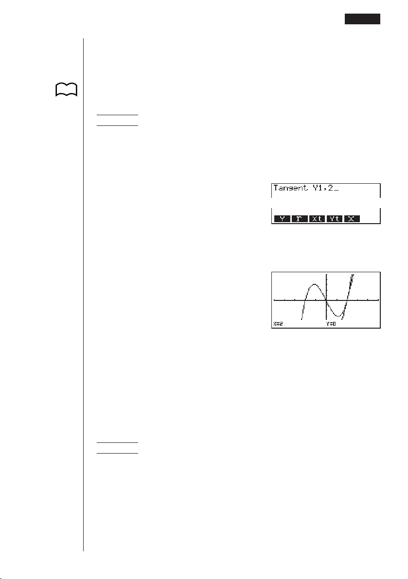
177
uu
uu
uTo draw a tangent in the RUN or PRGM Mode
The following is the command syntax for drawing a tangent in these modes.
Tangent <graph function>, <
x-coordinate>
• Use the variable data (VARS) menu to specify the function to be graphed.
Example To draw a line that is tangent to point (x = 2, y = 0) of y = x(x + 2)
(x – 2)
1. Enter the RUN Mode, display the sketch menu, and then perform the following
input.
!4(Sketch)2(Tang)
J4(GRPH)
1(Y)b,c
2. Press w to draw the tangent line.
w
kk
kk
k Line Normal to a Curve
With this function you can draw a line that is normal to the curve at a specific point.
• A line that is normal to the curve at a given point is one that is perpendicular to
the tangent line at that point.
uu
uu
uTo draw a line normal to a curve in the GRAPH or TABLE Mode
Example To draw a line that is normal to the curve at point (x = 2, y = 0) of
y = x(x + 2)(x – 2)
1. After graphing the function, display the sketch menu and press 3 (Norm).
!4(Sketch)3(Norm)
Graphing with the Sketch Function 10 - 2
P.33
1 23456

178
2. Use the cursor keys (f , c, d, e ) to move the pointer the position of the
point where you want to draw the line.
e ~ e
3. Press w to draw the line.
w
uu
uu
uTo draw a line normal to a curve in the RUN or PRGM Mode
The following is the syntax for drawing a line normal to a curve in these modes.
Normal <graph function>, <x-coordinate>
• Use the variable data (VARS) menu to specify the function to be graphed.
kk
kk
k Graphing an Inverse Function
This function lets you graph the inverse of the function used to produce your original
graph.
uu
uu
uTo graph an inverse function in the GRAPH or TABLE Mode
Example To graph the inverse of y = x(x + 2)(x – 2)
After graphing the function, display the sketch menu and press 4 (Inv).
!4(Sketch)4(Inv)
• When graphing an inverse function when there is more than one graph function
stored in memory, select one of the functions and then press w.
10 - 2 Graphing with the Sketch Function
P.33

179
uu
uu
uTo graph an inverse function in the RUN or PRGM Mode
The following is the syntax for graphing an inverse function in these modes.
Inverse <graph function>
• Use the variable data (VARS) menu to specify the function to be graphed.
• You can only graph the inverse of functions whose graph type is specified as
rectangular coordinate type.
kk
kk
k Plotting Points
When plotting points on a graph, first display the sketch menu and then press 6
(g) 1 (PLOT) to display the plot menu.
6(g)1(PLOT)
1 (Plot) ........ Plot a point
2 (Pl•On) ..... Plot point at specific coordinates
3 (Pl•Off) ..... Delete point at specific coordinates
4 (Pl•Chg) ... Switch status of point at specific coordinates
uu
uu
uTo plot points in the STAT, GRAPH, TABLE, RECUR and CONICS
Modes
Example To plot a point on the graph of y = x(x + 2)(x – 2)
1. After graphing the function, display the sketch menu and perform the following
operation to cause the pointer to appear on the graph screen.
!4(Sketch)6(g)1(PLOT)1(Plot)
2. Use the cursor keys (f, c, d, e) to move the pointer the locations of the
points you want to plot and press w to plot.
• You can plot as many points as you want.
e ~ ef ~ f
w
• The current x- and y-coordinate values are assigned respectively to variables X
and Y.
Graphing with the Sketch Function 10 - 2
123456
P.33

180
uu
uu
uTo plot points in the RUN or PRGM Mode
The following is the syntax for plotting points in these modes.
Plot <
x-coordinate>, <y-coordinate>
Example To plot a point at (2, 2)
Use the following View Window parameters.
Xmin =–5 Ymin =–10
Xmax = 5 Ymax = 10
Xscale = 1 Yscale = 2
1. After entering the RUN Mode, display the sketch menu and perform the following
operation.
!4(Sketch)6(g)
1(PLOT)1(Plot)c,c
2. Press w and the pointer appears on the display. Press w again to plot a point.
ww
• You can use the cursor keys (f, c, d, e) to move the pointer around the
screen.
• If you do not specify coordinates, the pointer is located in the center of the
graph screen when it appears on the display.
• If the coordinates you specify are outside the range of the View Window param-
eters, the pointer will not be on the graph screen when it appears on the dis-
play.
• The current
x- and y-coordinate values are assigned respectively to variables X
and Y.
10 - 2 Graphing with the Sketch Function
1 23456

181
kk
kk
k Turning Plot Points On and Off
Use the following procedures to turn specific plot points on and off.
uu
uu
uTo turn plot points on and off in the STAT, GRAPH, TABLE, RECUR
and CONICS Modes
• To turn a plot point on
1. After drawing a graph, display the sketch menu and then perform the following
operation to make the pointer appear at the center of the screen.
!4(Sketch)6(g)1(PLOT)2(Pl•On)
2. Use the cursor keys (f, c, d, e) to move the pointer to the location where
you want to plot a point and then press w.
• To turn a plot point off
Perform the same procedure as described under “To turn a plot point on” above,
except press 3 (Pl•Off) in place of 2 (Pl•On).
• To change the on/off status of a plot point
Perform the same procedure as described under “To turn a plot point on” above,
except press 4 (Pl•Chg) in place of 2 (Pl•On).
uu
uu
uTo turn plot points on and off in the RUN or PRGM Mode
The following are the syntax for turning plot points on and off in these modes.
• To turn a plot point on
PlotOn <
x-coordinate>, <y-coordinate>
• To turn a plot point off
PlotOff <
x-coordinate>, <y-coordinate>
• To change the on/off status of a plot point
PlotChg <x-coordinate>, <y-coordinate>
Graphing with the Sketch Function 10 - 2

182
kk
kk
k Drawing a Line
To draw a line on a graph, first display the sketch menu and then press 6 (g) 2
(LINE) to display the line menu.
6(g)2(LINE)
1 (Line)........ Draw a line between two plotted points
2 (F•Line) .... Draw a line
uu
uu
uTo draw a line between two plotted points in the STAT, GRAPH,
TABLE, RECUR and CONICS Modes
Example To draw a line between the two points of inflection on the graph
of y = x(x + 2)(x – 2)
Use the same View Window parameters as in the example on page
176.
1. After graphing the function, display the sketch menu and perform the following
operation to cause the pointer to appear on the graph screen.
!4(Sketch)6(g)1(PLOT)1(Plot)
2. Use the cursor keys (f, c, d , e) to move the pointer to one of the points of
inflection and press w to plot it.
d ~ df ~ f
w
3. Use the cursor keys to move the pointer to the other point of inflection.
e ~ ec ~ c
10 - 2 Graphing with the Sketch Function
123456

183
4. Display the sketch menu and perform the following operation to draw a line be-
tween the two points.
!4(Sketch)6(g)
2(LINE)1(Line)
uu
uu
uTo draw a line in the STAT, GRAPH, TABLE, RECUR and CONICS
Modes
Example To draw a line between two points of inflection on the graph of
y = x(x + 2)(x – 2)
1. After graphing the function, display the sketch menu and perform the following
operation to cause the pointer to appear on the graph screen.
!4(Sketch)6(g)2(LINE)2(F•Line)
2. Use the cursor keys (f, c, d , e) to move the pointer to one of the points of
inflection and press w.
d ~ df ~ f
w
3. Use the cursor keys to move the pointer to the other point of inflection and press
w to draw the line.
e ~ ec ~ c
w
uu
uu
uTo draw a line in the RUN or PRGM Mode
The following is the syntax for drawing lines in these modes.
F-Line <x-coordinate 1>, <y-coordinate 1>, <x-coordinate 2>, <y-coordinate 2>
Graphing with the Sketch Function 10 - 2

184
kk
kk
k Drawing a Circle
You can use the following procedures to draw a circle on a graph.
uu
uu
uTo draw a circle in the STAT, GRAPH, TABLE, RECUR and CONICS
Modes
Example To draw a circle with a radius of R = 1 centered at point (1, 0)
on the graph of y = x(x + 2)(x – 2)
1. After graphing the function, display the sketch menu and perform the following
operation to cause the pointer to appear on the graph screen.
!4(Sketch)6(g)3(Crcl)
2. Use the cursor keys (f, c, d, e) to move the pointer to the location where
you want the center point of the circle to be and press w to plot it.
e ~ e
w
3. Use the cursor keys to move the pointer to a point on the circumference of the
circle (here to point x = 0) and then press w to draw the circle.
d ~ d
w
uu
uu
uTo draw a circle in the RUN or PRGM Mode
The following is the syntax for drawing circles in these modes.
Circle <center point
x-coordinate>, <center point y-coordinate>, <radius R value>
• Certain View Window parameters can make a circle appear as an ellipse.
10 - 2 Graphing with the Sketch Function

185
kk
kk
k Drawing Vertical and Horizontal Lines
The procedures presented here draw vertical and horizontal lines that pass through
a specific coordinate.
uu
uu
uTo draw vertical and horizontal lines in the STAT, GRAPH, TABLE,
RECUR and CONICS Modes
Example To draw a vertical line on the graph of y = x(x + 2)(x – 2)
1. After graphing the function, display the sketch menu and perform the following
operation to display the pointer and draw a vertical line through its current loca-
tion.
!4(Sketch)6(g)4(Vert)
2. Use the d and e cursor keys to move the line left and right, and press w to
draw the line at the current location.
e ~ e
w
To draw a horizontal line, simply press 5 (Hztl) in place of 4 (Vert), and use the
f and c cursor keys to move the horizontal line on the display.
uu
uu
uTo draw vertical and horizontal lines in the RUN or PRGM Mode
The following is the syntax for drawing vertical and horizontal lines in these modes.
• To draw a vertical line
Vertical <
x-coordinate>
• To draw a horizontal line
Horizontal <y-coordinate>
kk
kk
k Freehand Drawing
This function lets you make freehand drawings on a graph, just as if you were using
a pen.
• Freehand drawing is available only in the STAT, GRAPH, TABLE, RECUR and
CONICS Modes.
Graphing with the Sketch Function 10 - 2

186
Example To draw on the graph of y = x(x + 2)(x – 2)
1. After graphing the function, display the sketch menu and perform the following
operation to cause the pointer to appear on the graph screen.
!4(Sketch)6(g)6(g)1(PEN)
2. Use the cursor keys (f, c, d, e) to move the pointer to the location where
you want to start drawing and press w to plot it.
3. Use the cursor keys to move the pointer, drawing a line as it moves. Press w to
stop the draw operation of the pointer.
• Press A to quit the freehand draw operation.
kk
kk
k Comment Text
Use the following procedure to insert text for comments and labels into a graph.
uu
uu
uTo insert text in the STAT, GRAPH, TABLE, RECUR and CONICS
Modes
Example To insert the graph function as comment text into the graph of
y = x(x + 2)(x – 2)
1. After graphing the function, display the sketch menu and perform the following
operation to cause the pointer to appear on the graph screen.
!4(Sketch)6(g)6(g)2(Text)
2. Use the cursor keys (f, c, d, e) to move the pointer to the location where
you want to insert the comment text, and then input the text.
10 - 2 Graphing with the Sketch Function

187
e ~ ef ~ f
aY!=v
(v+c)(v-c)
uu
uu
uTo insert text in the RUN or PRGM Mode
The following is the syntax for inserting text in these modes.
Text <line number>, <column number>, “<text>”
• The line number can be specified within the range of 1 to 63, while the column
number can be specified in the range of 1 to 127.
• The following are the characters that can be used inside of comment text in the
STAT, GRAPH, TABLE, RECUR, or CONICS Mode.
A~Z, r,
θ
, space, 0~9, ., +, –, ×, ÷, (–), EXP, π, Ans, {, (, ), [, ], {, }, comma, →, x
2
,
^, log, In, ,
x
, 10
x
, e
x
,
3
, x
–1
, sin, cos, tan, sin
–1
, cos
–1
, tan
–1
• A newline operation cannot be performed when inserting comment text. To
input multiple lines, you have to perform the above comment text insert opera-
tions more than once.
kk
kk
k Turning Pixels On and Off
The following procedure lets you turn each individual screen pixel on and off. You
can specify any pixel from the upper left-hand corner (1, 1) to the lower right-hand
corner (63, 127) of the screen.
Line range: 1 to 63
Column range: 1 to 127
• Note that you can turn pixels on and off only in the RUN and PRGM Modes.
When turning pixels on and off, first display the sketch menu and then press 6 (g)
6 (g) 3 (PIXL) to display the pixel menu.
6(g)6(g)3(PIXL)
1 (On).......... Turn specified pixel on
2 (Off) .......... Turn specified pixel off
3 (Chg)........ Switch status of specified pixel
Graphing with the Sketch Function 10 - 2
123456

188
uu
uu
uTo turn pixels on and off
• To turn a pixel on
PxlOn <line number>, <column number>
• To turn a pixel off
PxlOff <line number>, <column number>
• To change the on/off status of a pixel
PxlChg <line number>, <column number>
uu
uu
uTo check the on/off status of a pixel
While the sketch menu is on the screen, press 6 (g) 6 (g) 4 (Test) and then
input the command shown below to check the status of the specified pixel. 1 is
returned when the pixel is on, and 0 is returned when the pixel is off.
PxlTest <line number>, <column number>
• Specify a line in the range of 1 to 63 and a column in the range of 1 to 127.
• Trying to perform one of the above operations without specifying a line and
column number results in an error (Syn ERROR).
• Pixel operations are valid only within the allowable line and column ranges.
kk
kk
k Clearing Drawn Lines and Points
The following operation clears all drawn lines and points from the screen.
uu
uu
uTo clear lines and points in the STAT, GRAPH, TABLE, RECUR and
CONICS Modes
Lines and points drawn using sketch menu functions are temporary. Display the
sketch menu and press 1 (Cls) to clear drawn lines and points, leaving only the
original graph.
uu
uu
uTo clear drawn lines and points in the RUN or PRGM Mode
The following is the syntax for clearing drawn lines and points, as well as the graph
itself.
Cls EXE
10 - 2 Graphing with the Sketch Function

Dual Graph
Dual Graph lets you split the display between two different screens,
which you can then use to draw different graphs at the same time.
Dual Graph gives you valuable graph analysis capabilities.
• You should be familiar with the contents of “8-3 Graph Function
Operations” before reading this chapter.
11-1 Before Using Dual Graph
11-2 Specifying the Left and Right View Window
Parameters
11-3 Drawing a Graph in the Active Screen
11-4 Displaying a Graph in the Inactive Screen
Chapter
11

190
11-1 Before Using Dual Graph
From the Main Menu, enter the GRAPH Mode and set the Dual Screen setting to
“Graph”.
!Zcc1(Grph)
J
• For further details about the function key menu at the bottom of the display, see
“8-1 Before Trying to Draw a Graph”.
• 8,192 bytes of memory are used whenever you set the Dual Screen setting to
“Graph”.
kk
kk
k About Dual Graph Screen Types
The screen on the left side of the display is called the
active screen
, and the graph
on the left side of the display is called the
active graph
. Conversely, the right side is
the
inactive screen
containing the
inactive graph
. Any function that you execute while
using Dual Graph is always applied to the active graph. To execute a function on the
right-side inactive graph, you must first make it active by moving it into the active
screen.
Active Screen
Actual graph drawing is done here.
Inactive Screen
Use this screen to make copies of active screen
graphs, and for the result of Zoom operations.
You can also set different View Window param-
eters for the active and inactive screens.
P.8
1 23456
123456
P.126

191
• Indicators appear to the right of the formulas in the function memory list to tell
where graphs are drawn with Dual Graph.
Indicates inactive graph (on right side of display)
Indicates graph drawn on both sides of display
If you redraw graphs in the situation shown above, the function marked “
R
” is
drawn as the inactive graph, while “
B
” is drawn using both sides of the display.
If you press 1 (SEL), the “
R
” and “
B
” indicators are cleared, and the graphs
are drawn as active graphs.
Before Using Dual Graph 11 - 1

192
11-2 Specifying the Left and Right View Window
Parameters
You can specify different View Window parameteres for the left and right sides of the
graph display.
uu
uu
uTo specify View Window parameters
Press !3 (V-Window) to display the View Window parameter setting screen for
the active (left side) graph.
!3 (V-Window)
1 (INIT)........ Initialization of View Window values
2 (TRIG)...... Initialization of View Window values to match trigonometric units
3 (STD) ....... View Window standard settings
4 (STO) ....... Store settings in memory
5 (RCL) ....... Recall settings from memory
6
(RIGHT) ...
Swap active (left) screen and inactive (right) screen View
Window settings
6
(LEFT)
• Use the procedures described under “View Window (V-Window) Settings” to in-
put parameter values.
• Use the following key operations to change to different screens while inputting
View Window parameters for the left and right side screens.
While the View Window parameter setting screen for the active graph is shown:
6 (RIGHT).............. Displays the inactive graph View Window param-
eter setting screen
123456
P.127
P.129
P.129
P.130
P.130
P.130

193
While the View Window parameter setting screen for the inactive graph is shown:
6 (LEFT) ................ Displays the active graph View Window parameter
setting screen
Specifying the Left and Right View Window Parameters 11 - 2

194
11-3 Drawing a Graph in the Active Screen
You can draw graphs only in the active screen. You can then copy or move the graph
to the inactive screen.
uu
uu
uDrawing a graph in the active screen
Example To draw the graph of y = x (x + 1) (x – 1)
Use the following View Window parameters:
Input the function.
v(v+b)
(v-b)
Store the function.
w
Draw the graph.
6 (DRAW) or w
123456

195
11-4 Displaying a Graph in the Inactive Screen
There are two methods you can use to display a graph in the inactive screen. You
can copy a graph from the active screen to the inactive screen, or you can move the
graph from the active screen to the inactive screen. In both cases, you must first
draw the graph in the left-side active screen.
kk
kk
k Before Displaying a Graph in the Inactive Screen
After drawing a graph in the active screen, press K, and the Dual Graph function
menu appears at the bottom of the display.
K
1 (COPY) .... Copies active graph to inactive screen
2 (SWAP).... Switches active screen and inactive screen
3 (PICT) ...... Picture function
kk
kk
k Copying the Active Graph to the Inactive Screen
Example To draw the graph for y = x (x + 1) (x – 1) on the active screen and
the inactive screen
Use the following View Window parameters:
Active (Left) Screen Inactive (Right) Screen
View Window parameters View Window parameters
Assume that the function being graphed is stored in memory area Y1.
Draw the graph in the active
screen.
6(DRAW)
123456
P.159
123456

196
Copy the graph to the inactive (right) screen.
K1(COPY)
• The graph is reproduced using the inactive screen View Window parameters.
kk
kk
k Switching the Contents of the Active and Inactive Screens
Example To switch the screens produced by the preceding example
Switch the screens.
K2(SWAP)
• Note that using 2 (SWAP) to switch the screens also switches their View
Window parameters.
kk
kk
k Drawing Different Graphs on the Active Screen and
Inactive Screen
Example To draw the graphs of the following functions on the screens
noted:
Active Screen: y = x (x + 1) (x – 1)
Inactive Screen:
y = 2x
2
– 3
Use the View Window parameters shown below.
Active (Left) Screen Inactive (Right) Screen
View Window parameters View Window parameters
Assume that the functions being graphed are stored in memory areas Y1 and Y2.
11 - 4 Displaying a Graph in the Inactive Screen

197
123456
Displaying a Graph in the Inactive Screen 11 - 4
1 23456
Select the function for the graph that you want to end up in the inactive (right) screen.
1(SEL)
Draw the graph in the active screen.
6(DRAW)
Swap the screens so the graph is on the inactive (right) screen.
K2(SWAP)
Select the function for the graph that you want in the now-empty active (left) screen.
A1(SEL)
Draw the graph.
6(DRAW)
• At this point, you could perform a copy operation and superimpose the active
graph over the inactive graph.
123456

198
K1(COPY)
• Pressing !6 (G ↔ T) lets you switch between display of the active and
inactive graphs, using the entire display for each.
!6(G ↔ T)
!6(G ↔ T)
!6(G ↔ T)
11 - 4 Displaying a Graph in the Inactive Screen

199
kk
kk
k Other Graph Functions with Dual Graph
After drawing a graph using Dual Graph, you can use the trace, zoom, sketch and
scroll functions. Note, however, that these functions are available only for the active
(left) graph. For details on using these functions, see “8-6 Other Graphing Func-
tions”.
• To perform any of the above operations on the inactive graph, first move the
inactive graph to the active screen.
• The graph screen will not scroll while a trace operation is being performed on the
active graph.
The following shows some example operations using the zoom function.
Example 1 To use box zoom to enlarge the graph of y = x (x + 1) (x – 1)
Use the following View Window parameters for the active graph.
Assume that the function is already stored in memory area Y1.
Draw the graph.
6(DRAW) or w
Specify one corner of the area to be enlarged.
!2(Zoom)1(BOX)
c ~ ce ~ ew
• Use the cursor keys to move the pointer to the
location you want.
Displaying a Graph in the Inactive Screen 11 - 4
123456
P.146

200
Move the pointer to the other corner of the area to be enlarged.
f
~ fd ~ d
Enlarge the graph.
w
• The View Window parameters of the inactive screen are always changed by a
Zoom operation, so if there is a graph already on the inactive screen, it is cleared
before the result of the Zoom operation is drawn there.
11 - 4 Displaying a Graph in the Inactive Screen

Graph-to-Table
With this function, the screen shows both a graph and a table. You
can move a pointer around the graph and store its current coordi-
nates inside the table whenever you want. This function is very
useful for summarizing graph analysis results.
• Be sure to read “Chapter 8 Graphing” and “Chapter 9 Graph Solve”
before trying to perform any of the operations described in this
chapter.
12-1 Before Using Graph-to-Table
12-2 Using Graph-to-Table
12-3 Graph-to-Table Precautions
Chapter
12

202
12-1 Before Using Graph-to-Table
1. In the Main Menu, select the GRAPH icon and enter the GRAPH Mode. Next,
use the set up screen to set the Dual Screen item to “G to T”.
!Z
cc2(G to T)
2. Press J and the Graph-to-Table menu appears.
J
• For the meaning of the items in the function menu at the bottom of the screen,
see “8-1 Before Trying to Draw a Graph”.
• Whenever the set up screen’s Dual Screen item is set to “G to T”, you can only
store rectangular coordinate (Y=), polar coordinate (r=), and parametric func-
tion graphs in memory.
• You cannot use Graph-to-Table to display split graph/table screens using
X=constant or inequality graphs of functions stored in the GRAPH or TABLE
Mode.
1 2 3456
P.8
P.126

203
12-2 Using Graph-to-Table
uu
uu
uTo store graph pointer coordinates in a table
• If the Derivative item in the set up screen is turned on, the following operation
also stores derivatives in the table.
Example To store the points of intersection and the coordinates for the
following graphs where X = 0:
Y1 = x
2
– 3
Y2 = –x + 2
Use the following View Window parameters.
Xmin = –5 Ymin = –10
Xmax = 5 Ymax = 10
Xscale = 1 Yscale = 2
1. Input the two functions.
2. Press 6 (DRAW) to draw the graph in the left half of the screen.
6(DRAW) or w
3. Press 1 (Trace) and then use e to move the pointer to the first intersection.
1(Trace)
e~e
4. Press w to store the coordinates of the pointer location in the table on the right
side of the screen.
w
P.6
123456
x
/
y
-coordinate value

204
5. Use e to move the pointer the point where X = 0 and then press w to store the
coordinates in the table.
e~e
w
e~e
w
6. Pressing A causes the cursor (k) to appear in the table. You can then use the
cursor keys to move the cursor around the table and check its values. Press A
again to return the pointer to the graph screen.
A
uu
uu
uTo save numeric table values in a list file
You can save columns of values into list files. Up to six values can be stored in a list
file.
• The cursor can be located in any row of the column whose data you want to save
in the list.
Example To save the x-coordinate data of the previous example in List 1.
1. Starting from the screen that appears in step 6 of the previous example, press K.
K
1 (CHNG).... Changes the active screen (between left and right)
2 (LMEM) .... Save table column to list file.
3 (PICT) ...... Save graph data to graph memory.
12 - 2 Using Graph-to-Table
P.159
123456

205
2. Press 2 (LMEM).
2(LMEM)
3. Press 1 (List1) to store the data in the x-coordinate column into List 1.
• Table data uses the same memory as TABLE menu table data.
• Always be sure to store table data into a list.
• Any of the following operations causes table data to be deleted.
• Editing expression data
• Changing set up screen or View Window settings
• Changing to a different mode
• If you save data into a list that already contains data, the previous data is re-
placed with the new data.
• For details on recalling numeric data saved in a list file, see “17. List Function”.
Using Graph-to-Table 12 - 2
1 23456
P.263

206
12-3 Graph-to-Table Precautions
• The only coordinates that can be saved in the table are those where the pointer
can move to using trace and graph solve.
• The only graph functions that can be used with a graph produced using the Graph-
to-Table are: trace, scroll, zoom, and graph solve (excluding integration calcula-
tions).
• Graph functions cannot be used while the cursor is blinking in the table. To clear
the cursor and make the graph side the active screen, press K 1 (CHNG).
• K key operation is disabled whenever a graph and table are both on the screen
and there is no numeric data in the table, and when the screen is not split (i.e.
when either the graph or table only is on the display).
• An error occurs if a graph for which a range is specified or an overwrite graph is
included among the graph expressions.

Dynamic Graph
The Dynamic Graph Mode of this calculator shows you real-time
representations of changes in a graph as coefficients and terms
are changed. It lets you see what happens to a graph when such
changes are made. For example, you can see the graph change as
illustrated here as the value of coefficient A changes in the formula
y = Ax
2
.
13-1 Before Using Dynamic Graph
13-2 Storing, Editing, and Selecting Dynamic Graph
Functions
13-3 Drawing a Dynamic Graph
13-4 Using Dynamic Graph Memory
13-5 Dynamic Graph Application Examples
Chapter
13

208
13-1 Before Using Dynamic Graph
In the Main Menu, select the DYNA icon and enter the DYNA Mode. When you do
the dynamic function list appears on the screen.
Selected memory area
Press
c
and
f
to move.
1 (SEL) ........ Dynamic Graph draw/non-draw status
2 (DEL) ........ Function delete
3 (TYPE) ..... Function type specification
4 (VAR) ........ Coefficient menu
5 (B•IN) ........ Menu of built-in functions*
6 (RCL) ........ Recall and execution of Dynamic Graph conditions and screen
data
* The built-in function menu contains the following seven functions.
•Y=AX+B
•Y=A(X+B)
2
+C
•Y=AX
2
+BX+C
•Y=AX^3+BX
2
+CX+D
•Y=Asin(BX+C)
•Y=Acos(BX+C)
•Y=Atan(BX+C)
P.210
P.218
123456

209
13-2 Storing, Editing, and Selecting Dynamic
Graph Functions
In addition to the seven built-in functions, you can input 20 of your own Dynamic
Functions. Once a function is stored in memory, it can be edited and selected when
needed for graphing.
All of the procedures you need to use for storing, editing, and selecting Dynamic
Graph functions are identical to those you use in the GRAPH Mode. For details, see
“8-3 Graph Function Operations”.
• Dynamic Graphs can be one of the following three types only: rectangular coor-
dinate (Y=), polar coordinate (r=), and parametric.
•You cannot use Dynamic Graph with X=constant or inequality graphs of func-
tions stored in the GRAPH or TABLE Mode.
• If you try to use Dynamic Graph with a function that does not contain a variable,
an error occurs “No Variable”. If this happens, press A to clear the error.
P.132

210
13-3 Drawing a Dynamic Graph
The following is the general procedure you should use to draw a Dynamic Graph.
1. Select or input a function.
2. Define the dynamic coefficient.
• This is a coefficient whose value changes in order to produce the different graphs.
• If the dynamic coefficient is already defined from a previous operation, you can
skip this step.
3. Assign values to each of the coefficients of the function.
4. Specify the range of the dynamic coefficient.
• If the range of the dynamic coefficient is already defined from a previous opera-
tion, you can skip this step.
5. Specify the speed of the draw operation.
• If the speed is already defined from a previous operation, you can skip this step.
6. Draw the Dynamic Graph.
uu
uu
uTo set Dynamic Graph conditions
Example To use Dynamic Graph to graph y = A (x–1)
2
–1 as the value of A
changes from 2 to 5 in increments of 1
Use the following View Window parameters.
Xmin = – 6.3 Ymin = – 3.1
Xmax = 6.3 Ymax = 3.1
Xscale = 1 Yscale = 1
1. Input the function you want to graph. Here we will edit a built-in function to input
our function.
5(B•IN)
c1(SEL)
1234 56
1 23456

211
2. Display the coefficient menu.
4(VAR) or w
Function being graphed
Coefficient whose value will change
Coefficients in function
1 (SEL) ........ Selects dynamic coefficient
2 (RANG) .... Dynamic coefficient range settings
3 (SPEED) ... Dynamic Graph drawing speed
5 (AUTO) ..... Automatic setting of end and pitch values to match coefficient
values
6 (DYNA) ..... Dynamic Graph draw operation
• The calculator automatically makes the first variable it finds the dynamic coeffi-
cient. To select a different coefficient, use c and f to move the highlighting to
the coefficient you want to use, and the press 1 (SEL).
• The letters representing each coefficient are variables, and so the values that
appears on the screen are those currently assigned to each variable. If a com-
plex number is assigned to a variable, only the integer part appears.
• All variables contained in the currently selected function appear on the display in
alphabetical order.
• If there is more than one function that can be drawn using Dynamic Graph, the
message “Too Many Functions” appears on the display.
• If the value of the dynamic variable is zero and you press 5 (AUTO), the dy-
namic variable automatically changes to 1 and Dynamic Graphing is performed.
3. Specify the value of each coefficient.
cw
-bw
-bw
• If there is more than one coefficient, use f and c to move the highlighting to
each coefficient and input its value.
•Values you input for coefficients are also assigned to the corresponding variable.
1234 56
1 2 3456
Drawing a Dynamic Graph 13 - 3

212
4. Recall the dynamic coefficient range setting menu.
2(RANG)
• The range you set remains in effect until you change it.
5. Change the range settings.
cw
J
• If you want to change the Dynamic Graph speed, press 3 (SPEED).
3(SPEED)
You can set the Dynamic Graph speed to any one of the following settings.
Stop & Go: Each step of the Dynamic Graph draw operation is performed each
time you press w.
Slow: 1/2 Normal
Normal: Default speed
Fast: Double Normal
1. Use f and c to move the highlighting to the speed you want to use.
2. Press 1 (SEL) to set the highlighted speed.
1 23456
13 - 3 Drawing a Dynamic Graph
Dynamic coefficient
Start value
End value
Increment
P.216

213
uu
uu
uTo start the Dynamic Graph draw operation
There are three different variations for Dynamic Graphing.
• 10-time continuous drawing
• Continuous drawing
• Stop and go drawing
kk
kk
k 10-time Continuous Drawing
Select Stop as the draw type (Dynamic Type) to perform 10-time continuous draw-
ing. With this drawing style, 10 versions of the graph are drawn and then the draw
operation stops automatically.
Example To use 10-time continuous drawing to draw the same graph that
you drew in the previous example (page 210)
Display the coefficient value specification display and specify Stop as the draw type.
!Z2(Stop)
J
Start drawing of the Dynamic Graph.
6(DYNA)
↓
Graph is drawn 10 times. ↓↑
Drawing a Dynamic Graph 13 - 3
1 2 3456
123456

214
↓↑
↓↑
• While the message “One Moment Please!” is shown on the display, you can
press A to interrupt drawing of the graph and return to the coefficient range
setting display.
• Pressing A while the Dynamic Graph is being drawn changes to the drawing
speed setting display. The draw operation is suspended at this time, and you can
view the graph by pressing !6 (G ↔ T).
• If you do not want the function and coefficient values shown on the display with
the graph, use the graph function set up display to switch Graph Func off.
• Pressing 5 (AUTO) draws up to 11 versions of the Dynamic Graph, starting
from the start (Start) value of the dynamic coefficient.
P. 7
13 - 3 Drawing a Dynamic Graph

215
kk
kk
k Continuous Drawing
When the Dynamic Graph draw type (Dynamic Type) is set to continuous (Cont),
drawing of the Dynamic Graph continues until you press A.
Example To continuously draw the same graph that you input in the
previous example (page 210)
Display the coefficient value specification display, and specify Cont as the draw type.
!Z1(Cnt)
J
Start drawing of the Dynamic Graph.
6(DYNA)
↑
↓
• Pressing A while the Dynamic Graph is being drawn changes to the drawing
speed setting display. The draw operation is suspended at this time, and you can
view the graph by pressing !6 (G ↔ T).
• Selecting Cont and then executing a Dynamic Graph operation causes the
graphing operation to repeat until you press A. Be sure that you do not forget to
stop the Dynamic Graph operation after you are finished. Allowing it to continue
will run down the batteries.
Drawing a Dynamic Graph 13 - 3
1 23456
123456

216
kk
kk
k Stop & Go Drawing
By selecting STOP & GO tg as the graph drawing speed, you can draw graphs one
by one. A graph is drawn each time you press w.
Example To use Stop & Go to draw the same graph that you drew in the
previous example (page 210)
Display the coefficient value specification display and press 3 (SPEED).
Use f and c to select STOP & GO (tg) and press 1 (SEL).
3(SPEED)ff
1(SEL)J
Start drawing of the Dynamic Graph.
6(DYNA)
w
↑
w
↓
• Pressing A while the Dynamic Graph is being drawn changes to the drawing
speed setting display. The draw operation is suspended at this time, and you can
view the graph by pressing !6 (G ↔ T).
13 - 3 Drawing a Dynamic Graph
123456

217
uu
uu
uTo adjust the Dynamic Graph speed
You can use the following procedure to adjust the Dynamic Graph speed while the
draw operation is taking place.
1. While a Dynamic Graph draw operation is being performed, press A to change
to the speed adjustment menu.
A
1 (tg) ........... Stop & Go
2 (>) ............. Slow (1/2 Normal)
3 (g) ............ Normal (default speed)
4 (h) ............ Fast (double Normal)
5 (STO) ....... Store graph conditions and screen data in Dynamic Graph
memory
6 (DEL) ........ Delete Dynamic Graph screen data
2. Press the function key (1 to 4) that corresponds to the speed you want to
change to.
•To clear the speed adjustment menu without changing anything, press w.
• Press ! 6 (G↔T) to return to the graph screen.
Drawing a Dynamic Graph 13 - 3
P.218
P.219
123456

218
13 - 3 Drawing a Dynamic Graph
13-4 Using Dynamic Graph Memory
You can store Dynamic Graph conditions and screen data in Dynamic Graph memory
for later recall when you need it. This lets you save time, because you can recall the
data and immediately begin a Dynamic Graph draw operation. Note that you can
store one set of data in memory at any one time.
The following is all of the data that makes up a set.
• Graph functions (up to 20)
• Dynamic Graph conditions
• Set up screen settings
•View Window contents
• Dynamic Graph screen
uu
uu
uTo save data in Dynamic Graph memory
1. While a Dynamic Graph draw operation is being performed, press A to change
to the speed adjustment menu.
A
2. Press 5 (STO) to store the data.
• If there is already data stored in Dynamic Graph memory, the above operation
replaces it with the new data.
uu
uu
uTo recall data from Dynamic Graph memory
1. Display the Dynamic Graph function list.
2. Press 6 (RCL) to recall all the data stored in Dynamic Graph memory.
• Data recalled from Dynamic Graph replaces the calculator’s current graph func-
tions, draw conditions, and screen data. The previous data is lost when it is re-
placed.
12345 6
123456

219
uu
uu
uTo delete Dynamic Graph screen data
A6(DEL)
Press 1 (YES) to delete the Dynamic Graph Screen data, or 6 (NO) to abort the
operation without deleting anything.
1 23456
Using Dynamic Graph Memory 13 - 4

220
13 - 4 Using Dynamic Graph Memory
1234 56
1 2 3456
13-5 Dynamic Graph Application Examples
Example To use Dynamic Graph to graph the parabolas produced by balls
thrown in the air at an initial velocity of 20m/second, at angles of
30, 45, and 60 degrees. (Angle: Deg)
Use the following View Window parameters.
Xmin = –1 Ymin = –1
Xmax = 42 Ymax = 16
Xscale = 5 Yscale = 2
With the initial velocity defined as V and the angle defined as
θ
, the parabolas can be
obtained using the following expressions.
X = Vcos
θ
T
Y = Vsin
θ
T – (1/2)gT
2
g = 9.8 meters per second
1. Input the functions, making sure to specify them a parametric (Param) type.
2. Display the coefficient menu and specify the dynamic coefficient.
4(VAR)daw
3. Display the coefficient range menu and specify the range values.
2(RANG)
dawgawbfw

221
4. Start the Dynamic Graph draw operation.
J6(DYNA)
↑
↓
Dynamic Graph Application Examples 13 - 5

222
13 - 5 Dynamic Graph Application Examples

Implicit Function Graphs
You can graph any one of the following types of implicit functions
using the calculator’s built-in functions.
• Parabolic graph
• Circle graph
• Elliptical graph
• Hyperbolic graph
14-1 Before Graphing an Implicit Function
14-2 Graphing an Implicit Function
14-3 Implicit Function Graph Analysis
14-4 Implicit Function Graphing Precautions
Chapter
14

224
14-1 Before Graphing an Implicit Function
kk
kk
k Entering the CONICS Mode
1. In the Main Menu, select the CONICS icon and enter the CONICS Mode. When
you do, the following built in function menu appears on the screen.
2. Use f and c to highlight the built-in function you want, and then press w.
The following nine functions are built in.
Graph Type Function
Parabola X = A (Y – K)
2
+ H
X = AY
2
+ BY + C
Y = A (X – H)
2
+ K
Y = AX
2
+ BX + C
Circle (X – H)
2
+ (Y – K)
2
= R
2
AX
2
+ AY
2
+ BX + CY + D = 0
Ellipse (X – H)
2
(Y – K)
2
–––––––– + –––––––– = 1
A
2
B
2
Hyperbola (X – H)
2
(Y – K)
2
–––––––– – –––––––– = 1
A
2
B
2
(Y – K)
2
(X – H)
2
–––––––– – –––––––– = 1
A
2
B
2

225
14-2 Graphing an Implicit Function
Example 1 To graph the circle (X – 1)
2
+ (Y – 1)
2
= 2
2
Use the following View Window parameters.
Xmin = –6.3 Ymin = –3.1
Xmax = 6.3 Ymax = 3.1
Xscale = 1 Yscale = 1
1. Select the function whose graph you want to draw.
cccc
2. Press w and the variable input screen appears.
w
Graph function
Function variables
• The values that appear are the values currently assigned to each variable, which
are general variables used by the calculator. If the values include an imaginary
part, only the real part appears on the display.
3. Assign values to each variable.
bw
bw
cw
• You can also use f and c to highlight a
variable and then input a value.
4. Press 6 (DRAW) to draw the graph.
6 (DRAW)
123456

226
• Certain View Window parameters can make a circle graph come out looking like
an ellipse. When this happens, you can use the graph correction function (SQR)
to make corrections and produce a perfect circle.
(X – 3)
2
(Y – 1)
2
Example 2 To graph the hyperbola –––––––––– – –––––––––– = 1
2
2
2
2
Use the following View Window parameters.
Xmin = –8 Ymin = –10
Xmax = 12 Ymax = 10
Xscale = 1 Yscale = 1
1. Select the function whose graph you want to draw.
ccccccc
2. Press w and the variable input screen appears.
w
3. Assign values to each variable.
cw
cw
dw
bw
4. Press 6 (DRAW) to draw the graph.
6 (DRAW)
123456
P.155
14 - 2 Graphing an Implicit Function

227
• A parabola is the locus of points equidistant from fixed line l and fixed point F
not on the line. Fixed point F is the “focus,” fixed line l is the “directrix,” the
horizontal line that passes through the focus directrix is the “axis of symmetry,”
the length of a straight line that intersects the parabola, passes through the
locus, and is parallel to fixed line l is the “latus rectum,” and point A where the
parabola intersects the axis of symmetry is the “vertex.”
• An ellipse is the locus of points the sum of the distances of each of which from
two fixed points F and F’ is constant. Points F and F’ are the “foci,” points A, A’,
B, and B’ where the ellipse intersects the x- and y-axes are the “vertexes,” the
x-coordinate values of vertexes A and A’ are called x-intercepts, and the y-
coordinate values of vertexes B and B’ are called y-intercepts.
• A hyperbola is the locus of points related to two given points F and F’ such that
the difference in distances of each point from the two given points is constant.
Points F and F’ are the “foci,” points A and A’ where the hyperbola intersects
the x-axis are the “vertexes,” the x-coordinate values of vertexes A and A’ are
called x-intercepts, the y-coordinate values of vertexes A and A’ are called y-
intercepts, and straight lines i and i' , which get closer to the hyperbola as they
move away from the foci are “asymptotes.”
Axis of symmetry
Latus rectum
Directrix
l
Vertex A
Focus F (p, 0)
Graphing an Implicit Function 14 - 2
x
-intercept A’
Focus F’ Focus F
x
-intercept A
y
-intercept B’
y
-intercept B
Focus F' Focus F
Vertex
A’
Vertex
A
Asymptote
l
Asymptote
l'

228
14-3 Implicit Function Graph Analysis
You can determine approximations of the following analytical results using implicit
function graphs.
• Focus/vertex calculation
• Latus rectum calculation
• Center/radius calculation
•
x-/y-intercept calculation
• Directrix/axis of symmetry drawing and analysis
• Asymptote drawing and analysis
After graphing an implicit function, press 5 (G-Solv) to display the Graph Analysis
Menu.
• Parabolic Graph Analysis
1 (FOCS) .... Determines the focus.
2 (SYM)....... Draws the axis of symmetry.
3 (DIR) ........ Draws the directrix.
4 (VTX) ....... Determines the vertex.
5 (LEN) ....... Determines the latus rectum.
• Circle Graph Analysis
1 (CNTR) .... Determines the center.
2 (RADS) .... Determines the radius.
• Ellipse Graph Analysis
1 (FOCS) .... Determines the focus.
2 (X-IN) ....... Determines the
x-intercept.
3 (Y-IN)........ Determines the y-intercept.
• Hyperbolic Graph Analysis
1 (FOCS) .... Determines the focus.
2 (X-IN) ....... Determines the
x-intercept.
3 (Y-IN)........ Determines the y-intercept.
4 (VTX) ....... Determines the vertex.
5 (ASYM) .... Determines the asymptote.
The following examples show how to use the above menus with various types of
implicit function graphs.
123456
123456
123456
123456

229
uu
uu
uTo calculate the focus and vertex
Example To determine the focus and vertex for the parabola
X = (Y – 2)
2
+ 3.
Use the following View Window parameters.
Xmin = –1 Ymin = –5
Xmax = 10 Ymax = 5
Xscale = 1 Yscale = 1
5 (G-Solv)
1 (FOCS)
(Calculates the focus.)
5 (G-Solv)
4 (VTX)
(Calculates the vertex.)
• When calculating two foci for an ellipse or hyperbolic graph, press e to calcu-
late the second focus. Pressing d returns to the first focus.
• When calculating two vertexes for a hyperbolic graph, press e to calculate the
second vertex. Pressing d returns to the first vertex.
uu
uu
uTo calculate the latus rectum
Example To determine the latus rectum for the parabola X = (Y – 2)
2
+ 3
Use the following View Window parameters.
Xmin = –1 Ymin = –5
Xmax = 10 Ymax = 5
Xscale = 1 Yscale = 1
5 (G-Solv)
1 23456
123456
123456
Implicit Function Graph Analysis 14 - 3

230
5 (LEN)
(Calculates the latus rectum.)
uu
uu
uTo calculate the center and radius
Example To determine the center and radius for the circle X
2
+ Y
2
– 2X –
2Y – 3 = 0
Use the following View Window parameters.
Xmin = –6.3 Ymin = –3.1
Xmax = 6.3 Ymax = 3.1
Xscale = 1 Yscale = 1
5 (G-Solv)
1 (CNTR)
(Calculates the center.)
5 (G-Solv)
2 (RADS)
(Calculates the radius.)
1 23456
123456
14 - 3 Implicit Function Graph Analysis

231
uu
uu
uTo calculate the x- and y-intercepts
Example To determine the x- and y-intercepts for the hyperbola
(X – 1)
2
(Y – 1)
2
–––––––––– – –––––––––– = 1
2
2
2
2
Use the following View Window parameters.
Xmin = –6.3 Ymin = –3.1
Xmax = 6.3 Ymax = 3.1
Xscale = 1 Yscale = 1
5 (G-Solv)
2 (X-IN)
(Calculates the
x-intercept.)
5 (G-Solv)
3 (Y-IN)
(Calculates the y-intercept.)
• Press e to calculate the second set of
x-/y-intercepts. Pressing d returns to
the first set of intercepts.
uu
uu
uTo draw and analyze the axis of symmetry and directrix
Example To draw the axis of symmetry and directrix for the parabola
X = 2(Y – 1)
2
+ 1
Use the following View Window parameters.
Xmin = –6.3 Ymin = –3.1
Xmax = 6.3 Ymax = 3.1
Xscale = 1 Yscale = 1
5 (G-Solv)
1 2 3456
123456
Implicit Function Graph Analysis 14 - 3
1 2 3456

232
2 (SYM)
(Draws the axis of symmetry.)
5 (G-Solv)
3 (DIR)
(Draws the axis of directrix.)
uu
uu
uTo draw and analyze the asymptotes
Example To draw the asymptotes for the hyperbola
(X – 1)
2
(Y – 1)
2
–––––––––– – –––––––––– = 1
2
2
2
2
Use the following View Window parameters.
Xmin = –6.3 Ymin = –5
Xmax = 6.3 Ymax = 5
Xscale = 1 Yscale = 1
5 (G-Solv)
5 (ASYM)
(Draws the asymptotes.)
• Certain View Window parameters can produce errors in graph analysis result
values.
• The message ”Not Found” appears on the display when graph analysis is
unable to produce a result.
• The following can result in inaccurate analysis results or may even make it
impossible to obtain a solution at all.
• When the solution is tangent to the
x-axis.
• When the solution is a point of tangency between two graphs.
123456
123456
14 - 3 Implicit Function Graph Analysis

233
14-4 Implicit Function Graphing Precautions
• Assigning the following types of values to variables contained in built-in function
produces an error.
(1) Parabola graph
A = 0
(2) Circle graph
R = 0 for (X – H)
2
+ (Y – K)
2
= R
2
A = 0 for AX
2
+ AY
2
+ BX + CY + D = 0
(3) Ellipse/hyperbola graph
A = 0 or B = 0
• You cannot overwrite implicit function graphs.
• The calculator automatically clears the screen before drawing a new implicit func-
tion graph.
• You can use trace, scroll, zoom, or sketch after graphing an implicit function.
However, an implicit function graph cannot be scrolled while using trace.
• You cannot incorporate graphing of an implicit function into a program.

Table & Graph
With Table & Graph, you can generate tables of discreet data from
functions and recursion formulas, and then use the values for
graphing. Because of this, Table & Graph makes it easy to grasp
the nature of numeric tables and recursion formulas.
15-1 Before Using Table & Graph
15-2 Storing a Function and Generating a Numeric Table
15-3 Editing and Deleting Functions
15-4 Editing Tables and Drawing Graphs
15-5 Copying a Table Column to a List
Chapter
15

236
15-1 Before Using Table & Graph
First select the TABLE icon on the Main Menu and then enter the TABLE Mode.
When you do, the table function list appears on the display.
1 (SEL)........ Numeric table generation/non-generation status
2 (DEL) ....... Function delete
3 (TYPE) ..... Function type specification
5 (RANG) .... Table range specification screen
6 (TABL)...... Start numeric table generation
• Note that the item for function key 5 (RANG) does not appear when a list name
is specified for the Variable item in the set up screen.
123456
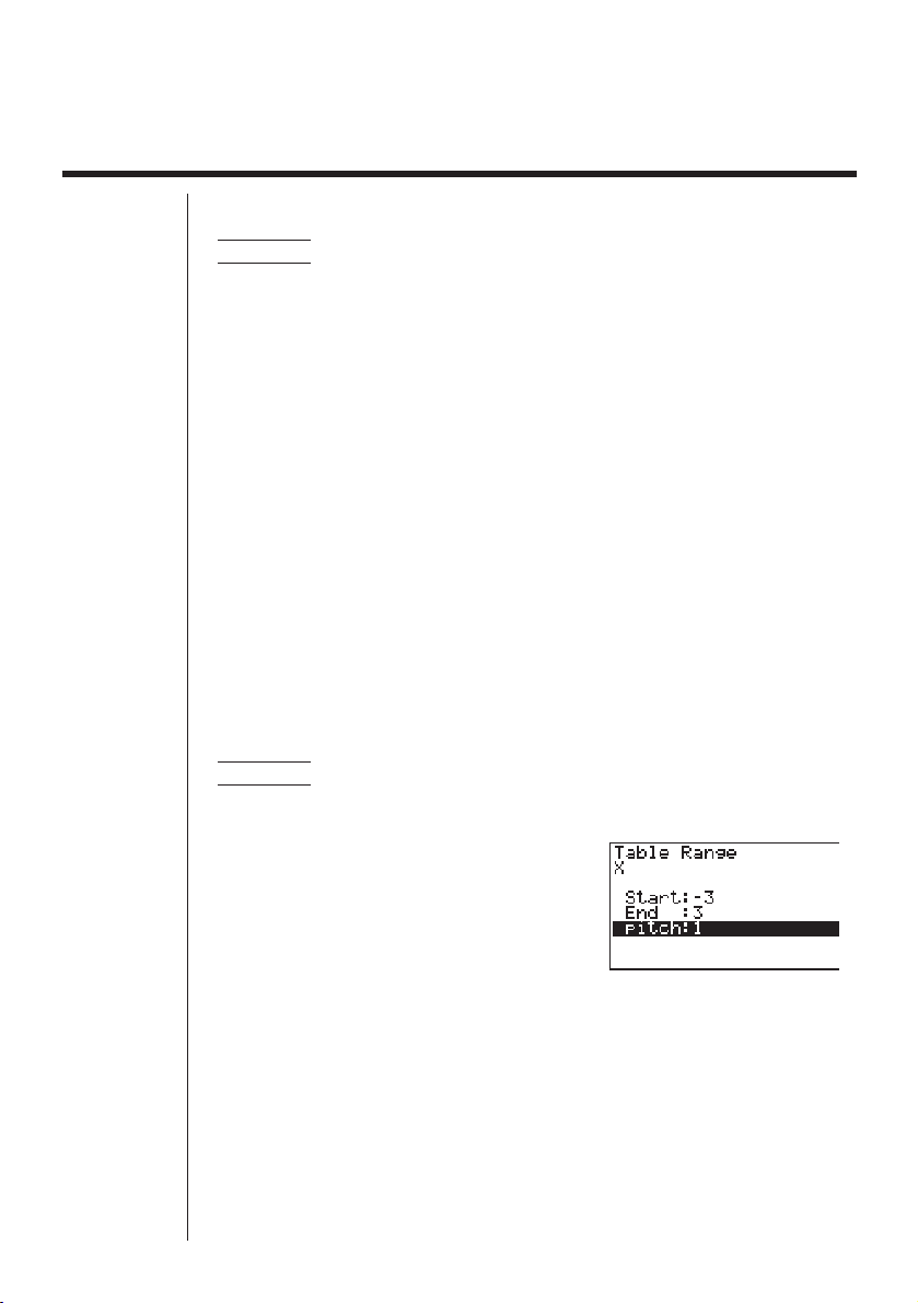
237
15-2 Storing a Function and Generating a Numeric
Table
uu
uu
uTo store a function
Example To store the function y = 3x
2
– 2 in memory area Y1
Use f and c to move the highlighting in the TABLE Mode function list to the
memory area where you want to store the function. Next, input the function and
press w to store it.
kk
kk
k Variable Specifications
There are two methods you can use to specify value for the variable x when gener-
ating a numeric table.
• Table range method
With this method, you specify the conditions for the change in value of the vari-
able.
• List
With this method, you substitute the values contained in a previously created list
for the value of the variable.
uu
uu
u To generate a table using a table range
Example To generate a table as the value of variable x change from –3 to 3,
in increments of 1
5(RANG)
-dwdwbw
The numeric table range defines the conditions under which the value of variable
x
changes during function calculation. The following is the meaning of each of the
numeric table range parameters.
Start................ Variable x start value
End ................. Variable x end value
pitch................ Variable x value change
After specifying the table range, press J to return to the function list.

238
uu
uu
uTo generate a table using a list
Example To generate a table using the values in List 6
!Z
• If the highlighting is not located at the Variable item, use f and c to move it
there.
2(LIST)6(List6)
After specifying the list you want to use, press J to return to the previous screen.
• Note that the RANG item for function key 5 of the TABLE Menu function list
does not appear when a list name is specified for the Variable item of the set up
screen.
kk
kk
k Generating a Table
Example To generate a table of values for the functions stored in
memory areas Y1 and Y3 of the TABLE Mode function list
Use f and c to move the highlighting to the function you want to select for table
generation and press 1 (SEL) to select it.
The “=” sign of selected functions are highlighted on the screen. To deselect a func-
tion, move the cursor to it and press 1 (SEL) again.
Press 6 (TABL) or w to generate a numeric table using the functions you se-
lected. The value of variable x changes according to the range or the contents of the
list you specified.
15 - 2 Storing a Function and Generating a Numeric Table
123456
123456

239
6(TABL)
Each cell can contain up to six digits, including negative sign.
You can use d, e, f, and c to move the highlighting around the table for the
following purposes.
• To display the selected cell’s value at the bottom of the screen, using the calcula-
tor’s current number of decimal place, number of significant digit, and exponential
display range settings.
• To scroll the display and view parts of the table that do not fit in the display.
• To display at the top of the screen the scientific function that produced the value
the selected cell (in columns Y1, Y2, etc.)
• To change
x variable values by replacing values in column X.
Press 1 (FORM) to return to the TABLE Mode function list.
uu
uu
uTo generate a differential numeric table
In the set up screen, change the setting of the Derivative item to On. Once you do
this, the derivative is shown on the display whenever you generate a numeric table.
• An error occurs if a graph for which a range is specified or an overwrite graph is
included among the graph expressions.
Storing a Function and Generating a Numeric Table 15 - 2
Locating the cursor at a differential
coefficient displays the derived function.
P.6

240
kk
kk
k Specifying the function type
You can specify a function as being one of three types.
• Rectangular coordinate
• Polar coordinate
• Parametric
To display the menu of function types, press 3 (TYPE) while the function list is on
the screen.
3(TYPE)
Press the function key (1, 2, 3) that corresponds to the function type you want
to specify.
• When you generate a numeric table, a table is generated only for the function
type you specify here.
123456
15 - 2 Storing a Function and Generating a Numeric Table

241
15-3 Editing and Deleting Functions
uu
uu
uTo edit a function
Example To change the function in memory area Y1 from y = 3x
2
– 2 to
y = 3x
2
– 5
Use f and c to move the highlighting to the function you want to edit.
Use d and e to move the cursor to the location of the change.
eeeeef
w
6(TABL)
• The Function Link Feature automatically reflects any changes you make to
functions in the TABLE Mode list in the GRAPH Mode and DYNA Mode lists.
uu
uu
uTo delete a function
Use f and c to move the highlighting to the function you want to delete and then
press 2 (DEL).
2(DEL)
Press 1 (YES) to delete the function or 6 (NO) to abort the operation without
deleting anything.
1 23456

242
15-4 Editing Tables and Drawing Graphs
You can use the table menu to perform any of the following operations once you
generate a table.
• Change the values of variable x
• Edit (delete, insert, and append) rows
• Delete a table
• Draw a connect type graph
• Draw a plot type graph
While the Table & Graph menu is on the display, press 6 (TABL) to display the
table menu.
6(TABL)
1 (FORM).... Display function list
2 (DEL) ....... Delete table
3 (ROW)...... Display menu of row operations
5 (G•CON) .. Draw connected type graph
6 (G•PLT) .... Draw plot type graph
uu
uu
uTo change variable values in a table
Example To change the value in Column x, Row 3 of the table generated
on page 239 from – 1 to – 2.5
cc
-c.f
w
123456
P.146

243
• When you change a variable value in Column
x, all values in the columns to the
right are recalculated and displayed.
• If you try to replace a value with an illegal operation (such as division by zero), an
Ma ERROR occurs and the original value remains unchanged.
• You cannot directly change any values in the other (non-x) columns of the table.
kk
kk
k Row Operations
The following menu appears whenever you press 3 (ROW) while the table menu
is on the display.
3(ROW)
1 (DEL) ....... Delete row
2 (INS) ........ Insert row
3 (ADD)....... Add row
uu
uu
uTo delete a row
Example To delete Row 2 of the table generated on page 239
3(ROW)c
1(DEL)
1 23456
123456
Editing Tables and Drawing Graphs 15 - 4

244
uu
uu
uTo insert a row
Example To insert a new row between Rows 1 and 2 in the table generated
on page 239
3(ROW)c
2(INS)
uu
uu
uTo add a row
Example To add a new row below Row 7 in the table generated on page 239
3(ROW)
cccccc
3(ADD)
kk
kk
k Deleting a Table
1. Display the table you want to delete and then press 2 (DEL).
2(DEL)
2. Press 1 (YES) to delete the table or 6 (NO) to abort the operation without
deleting anything.
1 2 3456
123456
123456
15 - 4 Editing Tables and Drawing Graphs

245
kk
kk
k Graphing a Function
uu
uu
uTo specify the draw/non-draw status of a formula
There are two options for the draw/non-draw status of a function graph.
• For the selected function only
• Overlay the graphs for all functions
To specify the draw/non-draw status, use same procedure as that for specifying
table generation/non-generation status.
uu
uu
uTo graph only a selected function
Example To graph y = 3x
2
– 2, which is stored in memory area Y1, as a
connect type graph.
Use the following View Window parameters.
Xmin = 0 Ymin = –2
Xmax = 6 Ymax = 106
Xscale = 1 Yscale = 2
c1(SEL)
(Specifies graph non-draw.)
6(TABL)
5(G•CON)
(Specifies connect type graph.)
Editing Tables and Drawing Graphs 15 - 4
123456
123456
No highlighting
P.238

246
uu
uu
uTo graph all of the functions
Example To use the values in the numeric table generated using the Table
Range and the View Window parameters from the previous ex-
ample to graph all functions stored in memory as plot type graphs.
6(TABL)
6(G•PLT)
(Specifies plot type graph.)
• After you graph a function, you can press !6 (G↔T) or A to return to the
function’s numeric table.
• After graphing a function, you can use the trace, zoom, sketch functions. For
details, see “8-6 Other Graph Functions”.
15 - 4 Editing Tables and Drawing Graphs
123456
P.146
123456

247
uu
uu
uTo graph a function using Dual Screen
Selecting “T+G” for the Dual Screen item of the set up screen makes it possible to
display both the graph and its numeric table of values.
Example To graph y = 3x
2
– 2 in memory are Y1, displaying both the graph
and its table
Use the same View Window parameters as in the example on page
245.
!Z
cc1(T+G)
(Specifies T+G for Dual Screen.)
J
6(TABL)
(Shows the table.)
6(G•PLT)
(Draws plot type graph.)
• Pressing !6 (G↔T) causes the graph on the left side of the Dual Screen to
fill the entire display. Note that you cannot use the sketch function while a graph
is displayed using !6 (G↔T).
P.8
Editing Tables and Drawing Graphs 15 - 4
1 23456
123456
123456

248
15-5 Copying a Table Column to a List
A simple operation lets you copy the contents of a numeric table column into a list.
uu
uu
uTo copy a table to a list
Example To copy the contents of Column x into List 1
K1(LIST)2(LMEM)
• You can select any row of the column you want to copy.
Press the function key (1 to 6) that corresponds the list you want to copy to.
1(List1)

Recursion Table and Graph
You can input two formulas for any of the three following types of
recursion, which you can then use to generate a table and draw
graphs.
• General term of sequence {an}, made up of an and n
• Formulas for linear recursion between two terms, made up of an+1,
an, and n
• Formulas for linear recursion between three terms, made up of
an+2, an+1, an, and n
16-1 Before Using the Recursion Table and Graph Function
16-2 Inputting a Recursion Formula and Generating a Table
16-3 Editing Tables and Drawing Graphs
Chapter
16

250
16-1 Before Using the Recursion Table and
Graph Function
uu
uu
uTo enter the RECUR Mode
On the Main Menu, select the RECUR icon and enter the RECUR Mode. This causes
the Recursion Menu to appear.
• All recursion formulas that are stored in memory appear in the Recursion Menu.
1 (SEL)........ Menu for control of table generation
2 (DEL) ....... Recursion formula delete
3 (TYPE) ..... Recursion formula type specification
4 (
n, an...) .... Menu for input of variable n and general terms an and bn
5 (RANG) .... Screen for setting of table range
6 (TABL)...... Recursion formula table generation
uu
uu
uTo specify the recursion formula type
Before inputting a recursion formula, you must first specify its type.
1. In the Recursion Menu, press 3 (TYPE).
3(TYPE)
• In this display, “an = An + B” is the general term (an = A × n + B) of {an}.
1 (an) ........... General term of sequence {an}
2 (an+1)......... Linear recursion between two terms
3 (an+2)......... Linear recursion between three terms
2. Press the function key for the recursion formula type you want to set.
123456
Selected storage area
Press
f
and
c
to move.
123456

251
16-2 Inputting a Recursion Formula and
Generating a Table
Example 1 To input an+1 = 2an + 1 and generate a table of values as the
value of n change from 1 to 6
Make
a1 = 1.
1. Specify the recursion formula type as linear recursion between two terms and
then input the formula.
c4(
n, an...)
2(an)+b
2. Press w and then press 5 (RANG) to display the table range setting screen.
w5(RANG)
1 (a0) ........... Value for a0 (b0)
2 (a1) ........... Value for a1 (b1)
The table range settings specify the conditions that control the value of variable
n in
the recursion formula, and the initial term of the numeric value table. You should also
specify a starting point for the pointer when drawing a convergence/divergence graph
(WEB graph) for a formula for linear recursion between two terms.
Start................ Starting value of variable n
End ................. Ending value of variable n
a
0, b0 ............... Value of 0th term a0/b0 (a1, b1 .... Value of 1st term a1/b1)
anStr, bnStr ...... Pointer starting point for convergence/divergence graph (WEB
graph)
• The value of variable n increments by 1.
3. Specify the range of the table.
2(
a1)
bwgwbw
1 2 3456
123456
P.258

252
4. Display the table of the recursion formula. At this time, a menu of table functions
appears at the bottom of the screen.
J6(TABL)
Value in currently highlighted cell
• Displayed cell values show positive integers up to six digits, and negative inte-
gers up to five digits (one digit used for negative sign). Exponential display can
use up to three significant digits.
• You can see the entire value assigned to a cell by using the cursor keys to move
the highlighting to the cell whose value you want to view.
• You can also display the sums of the terms
(Σan or Σbn) by turning on Σ Display.
Example 2 To input an+2 = an+1 + an (Fibonacci series) and generate a table
of values as the value of n change from 1 to 6
Make
a1 = 1 and a2 = 1.
1. Specify the recursion formula type as linear recursion between three terms and
then input the formula.
3(TYPE)3(an+2)
4(n, an...)
3(an+1)+2(an)
2. Press w and then press 5 (RANG) to display the table range setting screen.
w5(RANG)
1 (a0) ........... Value for a0 (b0) and a1 (b1)
2 (a1) ........... Value for a1 (b1) and a2 (b2)
P.9
16 - 2 Inputting a Recursion Formula and Generating a Table
1 23456
Currently selected cell (up to six digits)
123456

253
The table range settings specify the conditions that control the value of variable
n in
the recursion formula, and the initial term of the numeric value table.
Start................ Starting value of variable n
End ................. Ending value of variable n
a
0, a1, a2 .......... Values of 0th term a0/b0, 1st term a1/b1, and 2nd term a2/b2.
• The value of variable n increments by 1.
3. Specify the range of the table.
2(a1)
bwgwbwbw
4. Display the table of the recursion formula. At this time, a menu of table functions
appears at the bottom of the screen.
J6(TABL)
• There can be only one recursion table stored in memory at one time.
• Except for linear expression n, any of the following can be input for general
term {an} to generate a table: exponential expressions (such as an = 2
n
– 1),
fractional expressions (such as an = (n + 1)/n), irrational expressions (such as
an = n – ), trigonometric expressions (such as an = sin 2nπ).n – 1
• Note the following points when specifying a table range.
• If a negative value is specified as a start or end value, the calculator drops
the negative sign. If a decimal value or fraction is specified, the unit uses
only the integer part of the value.
• If the value of
a0/b0 (or a1/b1) is greater than the start value, the calculator
makes the starting value of variable x the same as the value of a0/b0 (or a1/
b1) before generating the table.
• If the start value is greater than the end value, the calculator swaps the two
values before generating the table.
• If the start value is the same as the end value, the calculator generates a
table using the start value of variable
x only.
• If the start value is very large, it may take a long time to generate a table for
linear recursion between two terms and linear recursion between three terms.
Inputting a Recursion Formula and Generating a Table 16 - 2
Currently selected cell (up to six digits)
Value in currently highlighted cell

254
16 - 2 Inputting a Recursion Formula and Generating a Table
123456
• Changing the angle unit setting while a table generated from a trigonometric
expression is on the display does not cause the displayed values to change. To
cause the values in the table to be updated using the new setting, display the
table, press 1 (FORM), change the angle unit setting, and then press 6
(TABL).
uu
uu
uTo specify the generation/non-generation status of a formula
Example To specify generation of a table for recursion formula an+1 = 2an+1
while there are two formulas stored
c1(SEL)
(Specifies non-generation status.)
Unhighlights this formula
6(TABL)
(Generates table.)
• To change the status of a recursion formula from non-generation to generation,
select the formula and press 1 (SEL).
uu
uu
uTo change the contents of a recursion formula
Changing the contents of a recursion formula causes the values in the table to be
updated using the current table range settings.
Example To change an+1 = 2an+1 to an+1 = 2an–3
e
(Displays the cursor.)
ee-dw
(Changes the formula contents.)
6(TABL)

255
uu
uu
uTo delete a recursion formula
1. Display the Recursion Menu and then use f and c to highlight the formula
you want to delete.
2. Press 2 (DEL).
3. Press 1 (YES) to delete the formula or 6 (NO) to abort the operation without
deleting anything.
Inputting a Recursion Formula and Generating a Table 16 - 2
1 23456

256
16-3 Editing Tables and Drawing Graphs
You get a choice of four options for editing tables and drawing graphs.
• Deletion of a recursion formula table
• Drawing of a connect type graph
• Drawing of a plot type graph
• Drawing of a graph and analysis of convergence/dievergence (WEB)
You can access these options from the function menu that appears at the bottom of
the screen whenever a table is displayed.
1 (FORM).... Returns to Recursion Menu.
2 (DEL) ....... Table delete
4 (WEB) ...... Draws convergence/divergence graph (WEB graph).
5 (G•CON) .. Draws connected type recursion graph.
6 (G•PLT) .... Draws plot type recursion graph.
• The WEB item (4) is available only when a table generated using a formula for
linear recursion between two terms (
an+1 =, bn+1 =) is on the display.
uu
uu
uTo delete a recursion table
1. Display the recursion table you want to delete and then press 2 (DEL).
2. Press 1 (YES) to delete the table or 6 (NO) to abort the operation without
deleting anything.
123456
P.259
P.146
P.146
1 23456

257
Editing Tables and Drawing Graphs 16 - 3
kk
kk
k Before Drawing a Graph for a Recursion Formula
You must first specify the following.
• Draw/non-draw status of for the recursion formula
• The type of data to be plotted
To specify the draw/non-draw status, display the Recursion Menu and then press
1 (SEL).
uu
uu
uTo specify the draw/non-draw status of a formula
There are two options for the draw/non-draw status of a recursion formula graph.
• Draw the graph for the selected recursion formula only
• Overly the graphs for both recursion formulas
To specify the draw/non-draw status, use same procedure as that for specifying
generation/non-generation status.
uu
uu
uTo specify the type of data to be plotted (Σ Display: On)
You can specify one of two types of data for plotting.
• an on the vertical axis, n on the horizontal axis
• Σan on the vertical axis, n on the horizontal axis
In the function menu that appears while a table is on the display, press 5 (G•CON)
or 6 (G•PLT) to display the Plot Data Menu.
1 (an) ........... an on the vertical axis, n on the horizontal axis
6 (Σan) ......... Σan on the vertical axis, n on the horizontal axis
Example 1 Draw a graph of an+1 = 2an + 1 with an on the vertical axis and n
on the horizontal axis, and with the points connected.
Set the following parameters in the View Window.
Xmin = 0 Ymin = 0
Xmax = 6 Ymax = 65
Xscale = 1 Yscale = 5
6(TABL)5(G•CON)
(Selects connected type.)
1 23456
P.254
1 23456

258
1(
an)
(Draws graph with an on the vertical
axis.)
Example 2 Draw a graph of an+1 = 2an + 1 with Σan on the vertical axis and n
on the horizontal axis, and with the points unconnected.
Use the same View Window parameters as those provided in Exam-
ple 1.
6(TABL)6(G•PLT)
(Selects plot type.)
6(Σ
an)
(Draws graph with Σan on the vertical
axis.)
• To input a different recursion formula after a graph is drawn, press ! Q. This
displays the Recursion Menu where you can input a new formula.
kk
kk
k Drawing a Convergence/Divergence Graph (WEB graph)
With this feature, you can draw a graph of an+1 = f
(an) where an+1 and an are the terms
of linear recursion between two terms, substituted respectively for y and x in the
function y = f
(x). The resulting graph can then be viewed to determine whether or not
the graph is convergent or divergent.
Example 1 To determine whether or not the recursion formula an+1 = –3an
2
+
3an is convergent or divergent.
Use the following table range.
Start = 0 End = 6
a0 = 0.01 an Str = 0.01
b0 = 0.11 bn Str = 0.11
Use the following View Window parameters.
Xmin = 0 Ymin = 0
Xmax = 1 Ymax = 1
Xscale = 1 Yscale = 1
16 - 3 Editing Tables and Drawing Graphs
123456

259
This example assumes that the following two recursion formulas are already stored
in memory.
1. Press 6 (TABL) to generate a table.
6(TABL)
2. Press 4 (WEB) to draw the graph.
4(WEB)
3. Press w, and the pointer appears at the pointer start point (anStr = 0.01).
w
• The Y value for the pointer start point is always 0.
4. Each press of w draws web-like lines on the display.
w
↓
w
↓
Editing Tables and Drawing Graphs 16 - 3
123456

260
16 - 3 Editing Tables and Drawing Graphs
This graph indicates that recursion formula an+1 = –3an
2
+ 3an is convergent.
Example 2 To determine whether or not the recursion formula bn+1 =
3bn + 0.2 is convergent or divergent.
Use the following table range.
Start = 0 End = 6
b0 = 0.02 bn Str = 0.02
Use the View Window parameters from Example 1.
1. Press 6 (TABL) 4 (WEB) to draw the graph.
6(TABL)
4(WEB)
2. Press w and then either f or c to make the pointer appear at the pointer
start point (bnStr = 0.02).
wc (or f)
• The Y value for the pointer start point is always 0.
123456

261
3. Each press of w draws web-like lines on the display.
w
↓
w
↓
This graph indicates that recursion formula bn+1 = 3bn + 0.2 is divergent.
• Inputting
bn or n for the expression an+1, or Inputting an or n for the expression bn+1
for linear recursion between two terms causes an error.
uu
uu
uTo draw a recursion formula graph using Dual Screen
Selecting “T+G” for the Dual Screen item of the Set Up Screen makes it possible to
display both the graph and its numerical table of values.
Example To draw the graph of an+1 = 2an + 1 from Example 1, displaying
both the graph and its table
!Z
ccc1(T+G)
(Specifies T+G for Dual Screen.)
J6(TABL)
(Draws the graph and shows the table.)
6(G•PLT)
(Draws plot type graph.)
• Pressing !6 (G↔T) causes the graph on the left side of the Dual Screen to
fill the entire display. Note that you cannot use the sketch function while a graph
is displayed using !6 (G↔T).
Editing Tables and Drawing Graphs 16 - 3
1 23456
P.8
P.258

List Function
A list is a kind of container that you can use to store multiple data items.
This calculator lets you store up to six lists in a single file, and you
can store up to six files in memory. Stored lists can be used in
arithmetic, statistical, and matrix calculations, and for graphing.
17-1 List Operations
17-2 Editing and Rearranging Lists
17-3 Manipulating List Data
17-4 Arithmetic Calculations Using Lists
17-5 Switching Between List Files
Chapter
17
Element number Display range Cell
Row
List name
Column
List 1 List 2 List 3 List 4 List 5 List 6
1 56 1 107 3.5 4 0
2 37 2 75 6 0 0
3 21 4 122 2.1 0 0
4 69 8 87 4.4 2 0
5 40 16 298 3 0 0
64832486.8 3 0
7 93 64 338 2 9 0
8 30 128 49 8.7 0 0
••••••
••••••
••••••
••••••

List Data Linking
264
Matrix Table
LIST
List operation
Example:
List 1 + List 2
{1, 2, 3} + {4, 5, 6}
List 1 + 3
From a graph to a list
Table data generated by
GRAPH TO TABLE to a list
↓
w
List internal operations
↓
w
Memory transfer
Generating a table by
defining a list as the
variable.
K
1(LIST)
2(LMEM)
4(List4)
Inside list
Copying the column of a
specific table to a specific list.
↓
w
Memory transfer
Example: To send column 1
of Mat A to a list
GraphOperation
List graphing
Y1=List 1X

265
17-1 List Operations
Select the LIST icon in the Main Menu and enter the LIST Mode to input data into a
list and to manipulate list data.
uu
uu
uTo input values one-by-one
Use d and e to move between lists, and f and c to move between cells
inside of a list.
The screen automatically scrolls when the cursor is located at the edge of the screen.
• c does not move the cursor to a cell that does not contain a value.
For our example, we will start by locating the cursor in Cell 1 of List 1.
1. Input a value and press w to store it in the list.
dw
2. The cursor automatically moves down to the next cell for input.
• Note that you can also use the result of an expression as list input. The next
operation shows how to input the value 4 in the second row and then input the
result of 2 + 3 in the next row.
ewc+dw

266
uu
uu
uTo batch input a series of values
1. Use f to move the cursor to the list name.
ffff
2. Use d or e to move the cursor to another list.
e
3. Press !{, and then input the values you want, pressing , between each
one. Press !} after inputting the final value.
!{g,h,i!}
4. Press w to store all of the values in your list.
w
• Remember that a comma separates values, so you should not input a comma
after the final value of the set you are inputting.
Right: {34, 53, 78}
Wrong: {34, 53, 78,}
You can also use list names inside of a mathematical expression to input values into
another cell. The following example shows how to add the values in each row in List
1 and List 2, and input the result into List 3.
1. Use d, e, f, and c to move the cursor to the name of the list where you
want the calculation results to be input.
fe
17 - 1 List Operations

267
2. Press K and input the expression.
K1(LIST)1(List)b+
1(List)cw
JJ
List Operations 17 - 1

268
17-2 Editing and Rearranging Lists
kk
kk
k Editing List Values
uu
uu
uTo change a cell value
Use d or e to move the cursor to the cell whose value you want to change. Input
the new value and press w to replace the old data with the new one.
uu
uu
uTo delete a cell
1. Use d, e, f, or c to move the cursor to the cell you want to delete.
ddc
2. Press 3 (DEL) to delete the selected cell and cause everything below it to be
shifted up.
3(DEL)
• Note that the above cell delete operation does not affect cells in other lists. If
the data in the list whose cell you delete is somehow related to the data in
neighboring lists, deleting a cell can cause related values to become misaligned.
uu
uu
uTo delete all cells in a list
1. Use d, e, f or c to move the cursor to the name of the list whose cells
you want to delete.
ffee
123456
123456

269
2. Press 4 (DEL-A). The function menu changes to confirm whether you really
want to delete all the cells in the list.
4(DEL-A)
3. Press 1 (YES) to delete all the cells in the selected list or 6 (NO) to abort the
delete operation without deleting anything.
1(YES)
uu
uu
uTo insert a new cell
Use d, e, f , or c to move the cursor to the location where you want to insert
the new cell. In this example, we will reinsert a cell containing the value 4, which we
deleted above.
1. Press 5 (INS) to insert a new cell, which contains a value of 0, causing every-
thing below it to be shifted down.
ddc5(INS)
2. Input the value you want into the new cell (4 in our example) and press w.
ew
• Note that the above cell insert operation does not affect cells in other lists. If the
data in the list where you insert a cell is somehow related to the data in
neighboring lists, inserting a cell can cause related values to become misaligned.
1 23456
Editing and Rearranging Lists 17 - 2
123456

270
kk
kk
k Sorting List Values
You can sort lists into either ascending order or descending order. The current cur-
sor location does not matter in the following procedures.
uu
uu
uTo sort a single list
Ascending order
1. While the lists are on the screen, press 1 (SRT-A).
1(SRT-A)
2. The prompt “How Many Lists? (H)” appears to ask how many lists you want to
sort. Here we will input 1 to indicate we want to sort only one list.
bw
3. In response to the “Select List (L)” prompt, input the number of the list you want to
sort. Here we will input 2 to specify sorting of List 2.
cw
The values in List 2 are sorted into ascending order.
Descending order
Use the same procedure as that for the ascending order sort. The only difference is
that you should press 2 (SRT-D) in place of 1 (SRT-A).
uu
uu
uTo sort multiple lists
You can link multiple lists together for a sort so that all of their cells are rearranged in
accordance with the sorting of a base list. The base list is sorted into either ascend-
ing order or descending order, while the cells of the linked lists are arranged so that
the relative relationship of all the rows is maintained.
17 - 2 Editing and Rearranging Lists

271
Ascending order
1. While the lists are on the screen, press 1 (SRT-A).
1(SRT-A)
2. The prompt “How Many Lists? (H)” appears to ask how many lists you want to
sort. Here we will sort one base list linked to one other list, so we should input 2.
cw
3. In response to the “Select Base List (B)” prompt, input the number of the list you
want to sort into ascending order. Here we will specify List 1.
bw
4. In response to the “Select Second List (L)” prompt, input the number of the list
you want to link to the base list. Here we will specify List 2.
cw
The values in List 1 are sorted into ascending order, and the cells of List 2 are also
rearranged to keep the same relationship with the List 1 cells.
Descending order
Use the same procedure as that for the ascending order sort. The only difference is
that you should press 2 (SRT-D) in place of 1 (SRT-A).
• You can sort up to six lists at one time.
• If you specify a list more than once for a single sort operation, an error occurs.
An error also occurs if lists specified for sorting do not have the same number of
values (rows).
Editing and Rearranging Lists 17 - 2

272
17-3 Manipulating List Data
List data can be used in arithmetic and function calculations. There is also a collec-
tion of powerful list data manipulation functions that let you do the following.
• Count the number values (Dim)
• Replace all cell values with the same value (Fill)
• Generate a sequence of numbers (Seq)
• Find the minimum value in a list (Min)
• Find the maximum value in a list (Max)
• Find which of two lists contains the smallest value (Min)
• Find which of two lists contains the greatest value (Max)
• Calculate the mean of list values (Mean)
• Calculate the mean of values of specified frequency (Mean)
• Calculate the median of values in a list (Med)
• Calculate the median of values of specified frequency (Med)
• Calculate the sum of values in a list (Sum)
• Calculate the sum of products (Prod)
• Calculate cumulative frequency of each value (Cuml)
• Calculate the percentage represented by each value (%)
• Transfer list contents to Matrix Answer Memory (List → Mat)
You use list data manipulation functions in the RUN, STAT, MAT, LIST, TABLE,
EQUA and PRGM Modes.
kk
kk
k Accessing the List Data Manipulation Function Menu
All of the following examples are performed after entering the RUN Mode.
Press K and then 1 (LIST). This menu has three pages and you can advance to
the next page by pressing 6 (g).
Note that all closing parentheses at the end of the following operations can be omitted.
uu
uu
uTo count the number of values (Dim)
K1(LIST)3(Dim)1(List) <list number 1-6> w
• The number of cells that contain data in a list is called its “dimension.”
Example To enter the RUN Mode and count the number of values in List 1
(36, 16, 58, 46, 56)
AK1(LIST)3(Dim)
1(List)bw

273
uu
uu
uTo replace all cell values with the same value (Fill)
K 1 (LIST) 4 (Fill) <value> , 1 (List) <list number 1-6> ) w
Example To replace all values in List 1 (36, 16, 58, 46, 56) with 3
AK1(LIST)4(Fill)
d,1(List)b)w
The following shows the new contents of List 1.
uu
uu
uTo generate a sequence of numbers (Seq)
K 1 (LIST) 5 (Seq) <expression> , <variable name> , <start
value> , <end value> , <pitch> ) w
• The result of this operation is also stored in ListAns Memory.
Example To input the number sequence 1
2
, 6
2
, 11
2
into a list
Use the following settings.
Variable:
x
Starting value: 1
Ending value: 11
Pitch: 5
AK1(LIST)5(Seq)v
x,v,b,bb,f)
w
Specifying an ending value of 12, 13, 14, or 15 produces the same result as shown
above, because all of them are less than the value produced by the next increment
(16).
The resulting sequence is input into ListAns Memory.
Manipulating List Data 17 - 3

274
uu
uu
uTo find the minimum value in a list (Min)
K 1 (LIST) 6 (g) 1 (Min) 6 (g) 6 (g) 1 (List) <list number
1-6> ) w
Example To find the minimum value in List 1 (36, 16, 58, 46, 56)
AK1(LIST)6(g)1(Min)
6(g)6(g)1(List)b)w
uu
uu
uTo find the maximum value in a list (Max)
Use the same procedure as when finding the minimum value (Min), except press
2 (Max) in place of 1 (Min).
uu
uu
uTo find which of two lists contains the smallest value (Min)
K 1 (LIST) 6 (g) 1 (Min) 6 (g)6 (g) 1 (List) <list number
1-6> , 1 (List) <list number 1-6> ) w
• The two lists must contain the same number of values. If they don’t, an error (Dim
ERROR) occurs.
• The result of this operation is also stored in ListAns Memory.
Example To find whether List 1 (75, 16, 98, 46, 56) or List 2 (36, 89, 58, 72,
67) contains the smallest value
K1(LIST)6(g)1(Min)
6(g)6(g)1(List)b,
1(List)c)
w
uu
uu
uTo find which of two lists contains the greatest value (Max)
Use the same procedure as that for the smallest value, except press 2 (Max) in
place of 1 (Min).
• The two lists must contain the same number of values. If they don’t, an error (Dim
ERROR) occurs.
uu
uu
uTo calculate the mean of list values (Mean)
K 1 (LIST) 6 (g) 3 (Mean) 6 (g) 6 (g) 1 (List) <list number 1-6>
) w
17 - 3 Manipulating List Data

275
Example To calculate the mean of values in List 1 (36, 16, 58, 46, 56)
AK1(LIST)6(g)3(Mean)
6(g)6(g)1(List)b)w
uu
uu
uTo calculate the mean of values of specified frequency (Mean)
This procedure uses two lists: one that contains values and one that contains the
number of occurrences of each value. The frequency of the data in Cell 1 of the first
list is indicated by the value in Cell 1 of the second list, etc.
• The two lists must contain the same number of values. If they don’t, an error (Dim
ERROR) occurs.
K 1 (LIST) 6 (g ) 3 (Mean) 6 (g ) 6 (g) 1 (List) <list number
1-6(data)> , 1 (List) <list number 1-6 (frequency)> ) w
Example To calculate the mean of values in List 1 (36, 16, 58, 46, 56), whose
frequency is indicated by List 2 (75, 89, 98, 72, 67)
AK1(LIST)6(g)3(Mean)
6(g)6(g)1(List)b,
1(List)c)w
uu
uu
uTo calculate the median of values in a list (Median)
K 1 (LIST) 6 (g) 4 (Med) 6 (g) 6 (g) 1 (List) <list number 1-6>
) w
Example To calculate the median of values in List 1 (36, 16, 58, 46, 56)
AK1(LIST)6(g)4(Med)
6(g)6(g)1(List)b)w
uu
uu
uTo calculate the median of values of specified frequency (Median)
This procedure uses two lists: one that contains values and one that contains the
number of occurrences of each value. The frequency of the data in Cell 1 of the first
list is indicated by the value in Cell 1 of the second list, etc.
• The two lists must contain the same number of values. If they don’t, an error (Dim
ERROR) occurs.
K 1 (LIST) 6 (g ) 4 (Med) 6 (g) 6 (g) 1 (List) <list number
1-6 (data)> , 1 (List) <list number 1-6 (frequency)> ) w
Manipulating List Data 17 - 3

276
Example To calculate the median of values in List 1 (36, 16, 58, 46, 56),
whose frequency is indicated by List 2 (75, 89, 98, 72, 67)
AK1(LIST)6(g)4(Med)
6(g)6(g)1(List)b,
1(List)c)w
uu
uu
uTo calculate the sum of values in a list (Sum)
K 1 (LIST) 6 (g) 6 (g) 1 (Sum) 6 (g) 1 (List) <list number 1-6> w
Example To calculate the sum of values in List 1 (36, 16, 58, 46, 56)
AK1(LIST)6(g)6(g)
1(Sum)6(g)1(List)bw
uu
uu
uTo calculate the sum of products (Prod)
K 1 (LIST) 6 (g) 6 (g) 2 (Prod) 6 (g) 1 (List) <list number
1-6> w
Example To calculate the sum of products for the values in List 1 (2, 3, 6, 5, 4)
AK1(LIST)6(g)6(g)
2(Prod)6(g)1(List)bw
uu
uu
uTo calculate the cumulative frequency of each value (Cuml)
K 1 (LIST) 6 (g) 6 (g) 3 (Cuml) 6 (g) 1 (List) <list number
1-6> w
Example To calculate the cumulative frequency of each value in List 1
(2, 3, 6, 5, 4)
The result is displayed in ListAns Memory.
AK1(LIST)6(g)6(g)
3(Cuml)6(g)1(List)b
w
2+3=
2+3+6=
2+3+6+5=
2+3+6+5+4=
17 - 3 Manipulating List Data

277
uu
uu
uTo calculate the percentage represented by each value (%)
K 1 (LIST) 6 (g) 6 (g) 4 (%) 6 (g) 1 (List) <list number
1-6> w
• The above operation calculates what percentage of the list total is represented
by each value.
Example To calculate the percentage represented by each value in List 1
(2, 3, 6, 5, 4)
The result is displayed in ListAns Memory.
AK1(LIST)6(g)6(g)
4(%)6(g)1(List)b
w
2/(2+3+6+5+4)
×
100 =
3
/
(
2+3+6+5+4
)
×
100 =
6
/
(
2+3+6+5+4
)
×
100 =
5
/
(
2+3+6+5+4
)
×
100 =
4
/
(
2+3+6+5+4
)
×
100 =
uu
uu
uTo transfer list contents to Matrix Answer Memory (List → Mat)
K1(LIST)2(L→M)1(List) <list number 1-6> ,1(List) <list
number 1-6> ) w
• You can input the following as many times as necessary to specify more than one
list in the above operation.
, <list number 1-6>
Example To transfer the contents of List 1 (2, 3, 6, 5, 4) and List 2 (11, 12,
13, 14, 15) to Matrix Answer Memory
AK1(LIST)2(L→M)
1(List)b,1(List)c)
w
Manipulating List Data 17 - 3

278
17-4 Arithmetic Calculations Using Lists
You can perform arithmetic calculations using two lists or one list and a numeric
value.
List
Numeric Value
List
Numeric Value
+
−
×
÷
=
List
ListAns Memory
kk
kk
k Error Messages
• A calculation involving two lists performs the operation between corresponding
cells. Because of this, a Dim ERROR occurs if the two lists do not have the same
number of values (which means they have different “dimensions”).
• An Ma ERROR occurs whenever an operation involving any two cells generates
a mathematical error.
kk
kk
k Inputting a List into a Calculation
There are two methods you can use to input a list into a calculation.
uu
uu
uTo input a specific list by name
Example To input List 6
1. Press K to display the first Operation Menu.
• This is the function key menu that appears in the RUN Mode when you press
K.
K
2. Press 1 (LIST) to display the List Data Manipulation Menu.
1(LIST)
3. Press 1 (List) to display the “List” command and input the number of the list you
want to specify.
1 23456
123456
Calculation results are
stored in ListAns Memory.

279
uu
uu
uTo directly input a list of values
You can also directly input a list of values using {, }, and ,.
Example 1 To input the list: 56, 82, 64
!{56,82,64!}
41 6
Example 2 To multiply List 3
(
= 65
)
by the list 0
22 4
K1(LIST)1(List)d*!{g,a,e!}w
246
The resulting list
0 is stored in ListAns Memory.
88
uu
uu
uTo assign the contents of one list to another list
Use a to assign the contents of one list to another list.
Example 1 To assign the contents of List 3 to List 1
K1(LIST)1(List)da1(List)bw
In place of 1 (List) d operation in the above procedure, you could input !{e
b,gf,cc!}.
Example 2 To assign the list in ListAns Memory to List 1
K1(LIST)1(List)!Ka1(List)bw
uu
uu
uTo input a single list cell value into a calculation
You can extract the value in a specific cell of a list and use it in a calculation. Specify
the cell number by enclosing it between square brackets using the [ and ] keys.
Example To calculate the sine of the value stored in Cell 3 of List 2
sK1(LIST)1(List)c![d!]w
Arithmetic Calculations Using Lists 17 - 4

280
uu
uu
uTo input a value into a specific cell
You can input a value into a specific cell inside a list. When you do, the value that
was previously stored in the cell is replaced with the new value you input.
Example To input the value 25 into cell 2 of List 3
cfaK1(LIST)1(List)d![c!]w
kk
kk
k Recalling List Contents
Example To recall the contents of List 1
K1(LIST)1(List)bw
• The above operation displays the contents of the list you specify and also stores
them in ListAns Memory. You can then use the ListAns Memory contents in a
calculation.
uu
uu
uTo use list contents in ListAns Memory in a calculation
Example To multiply the list contents in ListAns Memory by 36
K1(LIST)1(List)!K*dgw
• The operation K 1 (LIST) 1 (List) ! K recalls ListAns Memory contents.
• This operation replaces current ListAns Memory contents with the result of the
above calculation.
kk
kk
k Graphing a Function Using a List
When using the graphing functions of this calculator, you can input a function such
as Y1 = List1 X. If List 1 contains the values 1, 2, 3, this function will produces three
graphs: Y = X, Y = 2X, Y = 3X.
There are certain limitations on using lists with graphing functions.
kk
kk
k Inputting Scientific Calculations into a List
You can use the numeric table generation functions in the Table & Graph Menu to
input values that result from certain scientific function calculations into a list. To do
this, first generate a table and then use the list copy function to copy the values from
the table to the list.
17 - 4 Arithmetic Calculations Using Lists
P.126
P.248

281
kk
kk
k Performing Scientific Function Calculations Using a List
Lists can be used just as numeric values are in scientific function calculations. When
the calculation produces a list as a result, the list is stored in ListAns Memory.
41
Example 1 To use List 3 65 to perform sin (List 3)
22
Use radians as the angle unit.
sK1(LIST)1(List)dw
–0.158
The resulting list
0.8268 is stored in ListAns Memory.
–8E–3
In place of the 1 (List) d operation in the above procedure, you could input
!{ eb,gf,cc!}.
14
Example 2 To use List 1 2 and List 2 5 to perform List 1
List 2
36
List1MList2w
This creates a list with the results of 1
4
, 2
5
, 3
6
.
1
The resulting list
32 is stored in ListAns Memory.
729
Arithmetic Calculations Using Lists 17 - 4

282
17-5 Switching Between List Files
You can store up to six lists (List 1 to List 6) in each file (File 1 to File 6). A simple
operation lets you switch between list files.
uu
uu
uTo switch between list files
In the Main Menu, select the LIST icon and enter the LIST Mode.
Press ! Z to display the LIST Mode set up screen.
!Z
Press the function key (1 to 6) to select the file you want.
Example To select File 3
3(File3)
J
All subsequent list operations are applied to the lists contained in the file you select
(List File3 in the above example).
123456

Chapter
18
Statistical Graphs and
Calculations
This chapter describes how to input statistical data into lists, and
how to calculate the mean, maximum and other statistical values. It
also tells you how to perform regression calculations.
18-1 Before Performing Statistical Calculations
18-2 Paired-Variable Statistical Calculation Examples
18-3 Calculating and Graphing Single-Variable Statistical
Data
18-4 Calculating and Graphing Paired-Variable Statistical
Data
18-5 Other Graphing Functions
18-6 Performing Statistical Calculations
Important!
• This chapter contains a number of graph screen shots. In each case, new data
values were input in order to highlight the particular characteristics of the graph
being drawn. Note that when you try to draw a similar graph, the unit uses data
values that you have input using the List function. Because of this, the graphs
that appears on the screen when you perform a graphing operation will prob-
ably differ somewhat from those shown in this manual.

284
18-1 Before Performing Statistical Calculations
In the Main Menu, select the STAT icon to enter the STAT Mode and display the
statistical data lists.
Use the statistical data lists to input data and to perform statistical calculations.
1 (GRPH) .... Graph menu
2 (CALC)..... Statistical calculation menu
6 (g) ........... Next menu
6(g)
1 (SRT•A).... Ascending sort
2 (SRT•D) ... Descending sort
3 (DEL) ....... Single data item delete
4 (DEL•A).... Delete all data
5 (INS) ........ Insert data item
6 (g) ........... Previous menu
• The procedures you should use for data editing are identical to those you use
with the list function. For details, see “17. List Function”.
123456
123456
P.285
P.305
P.270
P.270
P.268
P.269
P.269
P.263
Use
f, c, d
and
e
to move
the highlighting around the lists.

285
18-2 Paired-Variable Statistical Calculation
Examples
Once you input data, you can use it to produce a graph and check for tendencies.
You can also use a variety of different regression calculations to analyze the data.
Example To input the following two data groups and perform statistical
calculations
0.5, 1.2, 2.4, 4.0, 5.2
–2.1, 0.3, 1.5, 2.0, 2.4
kk
kk
k Inputting Data into Lists
Input the two groups of data into List 1 and List 2.
a.fwb.cw
c.ewewf.cw
e
-c.bwa.dw
b.fwcwc.ew
Once data is input, you can use it for graphing and statistical calculations.
• Input values can be up to 10 digits long.
• You can use the f , c, d and e keys to move the highlighting to any cell in
the lists for data input.
kk
kk
k Plotting Data
Example To specify Graph 1 as non-draw (Off) and Graph 3 as draw (On)
and use Graph 3 to plot the data you input into statistical data
List 1 and List 2 above
While the statistical data list is on the display, press 1 (GRPH) to display the graph
menu.
1(GRPH)
1 (GPH1)..... Graph 1 draw
2 (GPH2)..... Graph 2 draw
3 (GPH3)..... Graph 3 draw
4 (SEL)........ Graph (GPH1, GPH2, GPH3) selection
6 (SET) ....... Graph settings (graph type, list assignments)
123456
P.287
P.288

286
• You can specify the graph draw/non-draw status, the graph type, and other gen-
eral settings for each of the graphs in the graph menu (GPH1, GPH2, GPH3).
• You can press any function key (1,2,3) to draw a graph regardless of the
current location of the highlighting in the statistical data list.
• The initial default graph type setting for all the graphs (Graph 1 through Graph 3)
is scatter diagram, but you can change to one of a number of other graph types.
kk
kk
k Plotting a Scatter Diagram
It is often difficult to spot the relationship between two sets of data (such as height
and shoe size) by simply looking at the numbers. Such relationships often become
clear however, when we plot the data on a graph, using one set as x-values and the
other set as y-values.
uu
uu
uTo plot a scatter diagram
Example To plot the data we input in statistical data List 1 and List 2
1(GPH1)
• The default setting automatically uses List 1 data as x-axis values and List 2 data
as y-axis values. Each set of x/y data is a point on the scatter diagram.
• To return to the statistical data list, press J or ! Q.
kk
kk
k Changing Graph Parameters
Use the following procedures to specify the graph draw/non-draw status, the graph
type, and other general settings for each of the graphs in the graph menu (GPH1,
GPH2, GPH3).
18 - 2 Paired-Variable Statistical Calculation Examples
P.287

287
1. Graph draw/non-draw status (SELECT)
The following procedure can be used to specify the draw (On)/non-draw (Off) status
of each of the graphs in the graph menu.
uu
uu
uTo specify the draw/non-draw status of a graph
1. While the graph menu is on the display, press 4 (SEL) to display the graph On/
Off screen.
1(GRPH)
4(SEL)
1 (On).......... Graph On (graph draw)
2 (Off).......... Graph Off (graph non-draw)
6 (DRAW).... Draw all On graphs
• Note that the StatGraph1 setting is for Graph 1 (GPH1 of the graph menu),
StatGraph2 is for Graph 2, and StatGraph3 is for Graph 3.
2. Use f and c to move the highlighting to the graph whose draw (On)/non-draw
(Off) status you want to change and press 1 (On) or 2 (Off).
3. To return to the graph menu, press J.
uu
uu
uTo draw a graph
Example To draw a scatter diagram of Graph 3 only
1(GRPH)4(SEL)
2(Off)
cc1(On)
6(DRAW)
123456
123456
Paired-Variable Statistical Calculation Examples 18 - 2

288
2. General graph settings (SET)
This section describes how to use the general graph settings screen to make the
following settings for each graph (GPH1, GPH2, GPH3).
• Graph Type
The initial default graph type setting for all the graphs is scatter graph. You can select
one of a variety of other statistical graph types for each graph.
• List
The initial default is statistical data List 1 for single-variable data, and List 1 and List
2 for paired-variable data. You can specify which statistical data list you want to use
for
x-data and y-data.
• Frequency
Normally, each data item or data pair in the statistical data list is represented on a
graph as a point. When you are working with a large number of data items however,
this can cause problems because of the number of plot points on the graph. When
this happens, you can specify a frequency list that contains values indicating the
number of instances (the frequency) of the data items in the corresponding cells of
the lists you are using for
x-data and y-data. Once you do this, only one point is
plotted for the multiple data items, which makes the graph easier to read.
• Mark Type
This setting lets you specify the shape of the plot points on the graph.
uu
uu
uTo display the general graph settings (SET) screen
While the graph menu is on the display, press 6 (SET) to display the general graph
settings screen.
1(GRPH)
6(SET)
• The settings shown here are examples only. The settings on your general graph
settings screen may differ.
uu
uu
uTo select the StatGraph area
1. While the general graph settings screen is on the display, use f and c to
move the highlighting to the StatGraph item.
123456
18 - 2 Paired-Variable Statistical Calculation Examples

289
2. Use the function key menu to select the StatGraph area you want to select.
1 (GPH1)..... Graph 1
2 (GPH2)..... Graph 2
3 (GPH3)..... Graph 3
uu
uu
uTo select the graph type (Graph Type)
1. While the general graph settings screen is on the display, use f and c to
move the highlighting to the Graph Type item.
2. Use the function key menu to select the graph type you want to select.
1 (Scat) ....... Scatter diagram
2 (
xy)........... xy line graph
6 (g) ........... Next menu
6(g)
1 (Hist) ........ Histogram (bar graph)
2 (Box) ........ Med-box graph
___
3 (Box) ........ Mean-box graph
4 (N•Dis) ..... Normal distribution curve
5 (Brkn) ....... Line graph
6 (g) ........... Next menu
6(g)
1 (X) ............ Linear regression graph
2 (Med) ....... Med-Med graph
3 (X^2) ........ Quadratic regression graph
4 (X^3) ........ Cubic regression graph
5 (X^4) ........ Quartic regression graph
6 (g) ........... Next menu
123456
123456
123456
Paired-Variable Statistical Calculation Examples 18 - 2

290
6(g)
1 (Log) ........ Logarithmic regression graph
2 (Exp) ........ Exponential regression graph
3 (Pwr) ........ Power regression graph
6 (g) ........... Previous menu
uu
uu
uTo select the x-axis data list (XList)
1. While the graph settings screen is on the display, use f and c to move the
highlighting to the XList item.
2. Use the function key menu to select the name of the statistical data list whose
values you want on the x-axis of the graph.
1 (List1)....... List 1
2 (List2)....... List 2
3 (List3)....... List 3
4 (List4)....... List 4
5 (List5)....... List 5
6 (List6)....... List 6
uu
uu
uTo select the y-axis data list (YList)
1. While the graph settings screen is on the display, use f and c to move the
highlighting to the YList item.
2. Use the function key menu to select the name of the statistical data list whose
values you want on the y-axis of the graph.
1 (List1)....... List 1
2 (List2)....... List 2
123456
123456
123456
18 - 2 Paired-Variable Statistical Calculation Examples

291
3 (List3)....... List 3
4 (List4)....... List 4
5 (List5)....... List 5
6 (List6)....... List 6
uu
uu
uTo select the frequency data list (Frequency)
1. While the general graph settings screen is on the display, use f and c to
move the highlighting to the Frequency item.
2. Use the function key menu to select the frequency setting you want.
1 (1) ............ Plot all data (1-to-1)
2 (List1)....... List 1 data is frequency data.
3 (List2)....... List 2 data is frequency data.
4 (List3)....... List 3 data is frequency data.
5 (List4)....... List 4 data is frequency data.
6 (g) ........... Next menu
6(g)
1 (List5)....... List 5 data is frequency data.
2 (List6)....... List 6 data is frequency data.
6 (g) ........... Previous menu
uu
uu
uTo select the plot mark type (Mark Type)
1. While the general graph settings screen is on the display, use f and c to
move the highlighting to the Mark Type item.
2. Use the function key menu to select the plot mark you want to select.
1 ( ) ........... Plot using
2 (X) ............ Plot using X
3 (•) ............. Plot using •
123456
123456
123456
Paired-Variable Statistical Calculation Examples 18 - 2

292
kk
kk
k Drawing an xy Line Graph
Paired data items can be used to plot a scatter diagram. A scatter diagram where the
points are linked is an xy line graph.
Press J or !Q to return to the statistical data list.
kk
kk
k Selecting the Regression Type
After you graph statistical data, you can use the function menu at the bottom of the
display to select from a variety of different types of regression.
1 (X) ............ Linear regression graph
2 (Med) ....... Med-Med graph
3 (X^2) ........ Quadratic regression graph
4 (X^3) ........ Cubic regression graph
5 (X^4) ........ Quartic regression graph
6 (g) ........... Next menu
6(g)
1 (Log) ........ Logarithmic regression graph
2 (Exp) ........ Exponential regression graph
3 (Pwr) ........ Power regression graph
4 (2VAR) ..... Paired-variable statistical results
6 (g) ........... Previous menu
18 - 2 Paired-Variable Statistical Calculation Examples
P.289
(Graph Type)
(xy)
123456
123456

293
kk
kk
k Displaying Statistical Calculation Results
Whenever you perform a regression calculation, the regression formula parameter
(such as a and b in the linear regression y = ax + b) calculation results appear on the
display. You can use these to obtain statistical calculation results.
Regression parameters are calculated as soon as you press a function key to select
a regression type while a graph is on the display.
Example To display logarithmic regression parameter calculation results
while a scatter diagram is on the display
6(g)1(Log)
kk
kk
k Graphing Statistical Calculation Results
You can use the parameter calculation result menu to graph the displayed regres-
sion formula.
5 (COPY) .... Stores the displayed regression formula as a graph function
6 (DRAW).... Graphs the displayed regression formula
Example To graph a logarithmic regression
While logarithmic regression parameter calculation results are on the display, press
6 (DRAW).
6(DRAW)
For details on the meanings of function menu items at the bottom of the display, see
“Selecting the Regression Type”.
123456
P.292
P.302
Paired-Variable Statistical Calculation Examples 18 - 2

294
18-3 Calculating and Graphing Single-Variable
Statistical Data
Single-variable data is data with only a single variable. If you are calculating the
average height of the members of a class for example, there is only one variable
(height).
Single-variable statistics include distribution and sum. The following five types of
graphs are available for single-variable statistics.
kk
kk
k Drawing a Histogram (Bar Graph)
From the statistical data list, press 1 (GRPH) to display the graph menu, press 6
(SET), and then change the graph type of the graph you want to use (GPH1, GPH2,
GPH3) to histogram (bar graph).
Data should already be input in the statistical data list (see “Inputting Data into List”).
Draw the graph using the procedure described under “Plotting Data”.
⇒
6(DRAW)
The display screen appears as shown above before the graph is drawn. At this
point, you can change the Start and pitch values.
kk
kk
k Med-box Graph (Med-Box)
This type of graph lets you see how a large number of data items are grouped within
specific ranges. A box encloses all the data in an area from the 25th percentile to the
75th percentile, with a line drawn at the 50th percentile. Lines (called whiskers)
extend from either end of the box up to the minimum and maximum of the data.
From the statistical data list, press 1 (GRPH) to display the graph menu, press 6
(SET), and then change the graph type of the graph you want to use (GPH1, GPH2,
GPH3) to med-box graph.
kk
kk
k Mean-box Graph
This type of graph shows the distribution around the mean when there is a large
number of data items. A line is drawn at the point where the mean is located, and
then a box is drawn so that it extends below the mean up to the standard deviation
and above the mean up to the standard deviation. Lines (called whiskers) extend
from either end of the box up to the minimum and maximum of the data.
P.285
P.289
(Graph Type)
(Hist)
123456
P.289
(Graph Type)
(Box)
P.289
(Graph Type)
(Box)

295
From the statistical data list, press 1 (GRPH) to display the graph menu, press 6
(SET), and then change the graph type of the graph you want to use (GPH1, GPH2,
GPH3) to mean-box graph.
kk
kk
k Normal Distribution Curve
The normal distribution curve is graphed using the following normal distribution func-
tion.
y
=
1
(2π) xσ
n
e
–
2xσ
n
2
(
x–
x
)
2
The distribution of characteristics of items manufactured according to some fixed
standard (such as component length) fall within normal distribution. The more data
items there are, the closer the distribution is to normal distribution.
From the statistical data list, press 1 (GRPH) to display the graph menu, press 6
(SET), and then change the graph type of the graph you want to use (GPH1, GPH2,
GPH3) to normal distribution.
kk
kk
k Line Graph
A line graph is formed by plotting the data in one list against the frequency of each
data item in another list and connecting the points with straight lines.
Calling up the graph menu from the statistical data list, pressing 6 (SET), changing
the settings to drawing of a line graph, and then drawing a graph creates a box
graph.
⇒
6(DRAW)
The display screen appears as shown above before the graph is drawn. At this
point, you can change the Start and pitch values.
Calculating and Graphing Single-Variable Statistical Data 18 - 3
P.289
(Graph Type)
(N•Dis)
P.289
(Graph Type)
(Brkn)
123456
Note :
This function is not usually used in
the classrooms in U.S. Please use
Med-box Graph, instead.

296
18 - 3 Calculating and Graphing Single-Variable Statistical Data
kk
kk
k Displaying Single-Variable Statistical Results
Single-variable statistics can be expressed as both graphs and parameter values.
When these graphs are displayed, the menu at the bottom of the screen appears as
below.
1 (1VAR) ..... Single-variable calculation result menu
Pressing 1 (1VAR) displays the following screen.
1(1VAR)
• Use c to scroll the list so you can view the items that run off the bottom of the
screen.
The following describes the meaning of each of the parameters.
_
x ..................... Mean of data
Σx ................... Sum of data
Σx
2
.................. Sum of squares
xσn .................. Population standard deviation
xσn-1 ................ Sample standard deviation
n ..................... Number of data items
minX ............... Minimum
Q1 .................. First quartile
Med ................ Median
Q3 .................. Third quartile
_
x –xσn ............ Data mean – Population standard deviation
_
x + xσn ............ Data mean + Population standard deviation
maxX .............. Maximum
Mod ................ Mode
• Press 6 (DRAW) to return to the original single-variable statistical graph.

297
18-4 Calculating and Graphing Paired-Variable
Statistical Data
Under “Plotting a Scatter Diagram,” we displayed a scatter diagram and then per-
formed a logarithmic regression calculation. Let’s use the same procedure to look at
the six regression functions.
kk
kk
k Linear Regression Graph
Linear regression plots a straight line that passes close to as many data points as
possible, and returns values for the slope and y-intercept (y-coordinate when x = 0)
of the line.
The graphic representation of this relationship is a linear regression graph.
!Q1(GRPH)6(SET)c
1(Scat)
!Q1(GRPH)1(GPH1)
1(X)
6(DRAW)
The following are the meanings of the above parameters.
a ...... Regression coefficient (slope)
b ...... Regression constant term (intercept)
r ...... Correlation coefficient
kk
kk
k Med-Med Graph
When it is suspected that there are a number of extreme values, a Med-Med graph
can be used in place of the least squares method. This is also a type of linear regres-
sion, but it minimizes the effects of extreme values. It is especially useful in produc-
ing highly reliable linear regression from data that includes irregular fluctuations,
such as seasonal surveys.
2(Med)
123456
P.289
(Graph Type)
(Scatter)
(GPH1)
(X)
P.289
123456

298
6(DRAW)
The following are the meanings of the above parameters.
a ...... Med-Med graph slope
b ...... Med-Med graph intercept
kk
kk
k Quadratic/Cubic/Quartic Regression Graph
A quadratic/cubic/quartic regression graph represents connection of the data points
of a scatter diagram. It actually is a scattering of so many points that are close
enough together to be connected. The formula that represents this is quadratic/
cubic/quartic regression.
Ex. Quadratic regression
3(X^2)
6(DRAW)
The following are the meanings of the above parameters.
Quadratic regression
a ...... Quadratic regression coefficient
b ...... Linear regression coefficient
c ...... Regression constant term (intercept)
Cubic regression
a ...... Cubic regression coefficient
b ...... Quadratic regression coefficient
c ...... Linear regression coefficient
d ...... Regression constant term (intercept)
123456
18 - 4 Calculating and Graphing Paired-Variable Statistical Data
P.289

299
Quartic regression
a ...... Quartic regression coefficient
b ...... Cubic regression coefficient
c ...... Quadratic regression coefficient
d ...... Linear regression coefficient
e ...... Regression constant term (intercept)
kk
kk
k Logarithmic Regression Graph
Logarithmic regression expresses y as a logarithmic function of x. The standard
logarithmic regression formula is y = a + b × logx, so if we say that X = logx, the
formula corresponds to linear regression formula y = a + bX.
6(g)1(Log)
6(DRAW)
The following are the meanings of the above parameters.
a ...... Regression constant term (intercept)
b ...... Regression coefficient (slope)
r ...... Correlation coefficient
kk
kk
k Exponential Regression Graph
Exponential regression expresses y as a proportion of the exponential function of x.
The standard exponential regression formula is y = a × e
bx
, so if we take the loga-
rithms of both sides we get logy = loga + bx. Next, if we say Y = logy, and a = loga,
the formula corresponds to linear regression formula Y = a + bx.
6(g)2(Exp)
123456
123456
Calculating and Graphing Paired-Variable Statistical Data 18 - 4
P.290
P.290

300
6(DRAW)
The following are the meanings of the above parameters.
a ...... Regression coefficient
b ...... Regression constant term
r ...... Correlation coefficient
kk
kk
k Power Regression Graph
Exponential regression expresses y as a proportion of the power of x. The standard
power regression formula is y = a × x
b
, so if we take the logarithms of both sides we
get logy = loga + b × logx. Next, if we say X = log x, Y = logy, and a = loga, the
formula corresponds to linear regression formula Y = a + bX.
6(g)3(Pwr)
6(DRAW)
The following are the meanings of the above parameters.
a ...... Regression coefficient
b ...... Regression power
r ...... Correlation coefficient
123456
18 - 4 Calculating and Graphing Paired-Variable Statistical Data
P.290

301
kk
kk
k Displaying Paired-Variable Statistical Results
Paired-variable statistics can be expressed as both graphs and parameter values.
When these graphs are displayed, the menu at the bottom of the screen appears as
below.
4(2VAR) ...... Paired-variable calculation result menu
Pressing 4 (2VAR) displays the following screen.
4(2VAR)
• Use c to scroll the list so you can view the items that run off the bottom of the
screen. The following describes the meaning of each of the parameters.
_
x ..................... Mean of xList data
Σ
x ................... Sum of xList data
Σx
2
.................. Sum of squares of xList data
xσn .................. Population standard deviation of xList data
xσn-1 ................ Sample standard deviation of xList data
n ..................... Number of xList data items
_
y ..................... Mean of yList data
Σy ................... Sum of yList data
Σ
y
2
.................. Sum of squares of yList data
yσn .................. Population standard deviation of yList data
yσn-1 ................ Sample standard deviation of yList data
Σxy ..................Sum of xList and yList data
minX ............... Minimum of
xList data
maxX .............. Maximum of xList data
minY ............... Minimum of yList data
maxY .............. Maximum of
yList data
123456
Calculating and Graphing Paired-Variable Statistical Data 18 - 4
P.290

302
kk
kk
k Copying a Regression Graph Formula to the Graph Mode
After you perform a regression calculation, you can copy its formula to the GRAPH
Mode.
The following are the functions that are available in the function menu at the bottom
of the display while regression calculation results are on the screen.
5 (COPY) .... Stores the displayed regression formula to the GRAPH Mode
6 (DRAW).... Graphs the displayed regression formula
1. Press 5 (COPY) to copy the regression formula that produced the displayed
data to the GRAPH Mode.
5(COPY)
Note that you cannot edit regression formulas for graph formulas in the GRAPH
Mode.
2. Press w to save the copied graph formula and return to the previous regression
calculation result display.
kk
kk
k Multiple Graphs
You can draw more than one graph on the same display by using the procedure
under “Changing Graph Parameters” to set the graph draw (On)/non-draw (Off) sta-
tus of two or all three of the graphs to draw (On), and then pressing 6 (DRAW).
After drawing the graphs, you can select which graph formula to use when perform-
ing single-variable statistic or regression calculations.
123456
P.286
123456
18 - 4 Calculating and Graphing Paired-Variable Statistical Data

303
6(DRAW)
1(X)
• The text at the top of the screen indicates the currently selected graph (StatGraph1
= Graph 1, StatGraph2 = Graph 2, StatGraph3 = Graph 3).
1. Use f and c to change the currently selected graph. The graph name at the
top of the screen changes when you do.
c
2. When graph you want to use is selected, press w.
Now you can use the procedures under “Displaying Single-Variable Statistical Re-
sults” and “Displaying Paired-Variable Statistical Results” to perform statistical cal-
culations.
P.296
P.301
Calculating and Graphing Paired-Variable Statistical Data 18 - 4
P.289

304
18-5 Other Graphing Functions
kk
kk
k Manual Graphing
In all of the graphing examples up to this point, values were calculated in accord-
ance with View Window settings and graphing was performed automatically. This
automatic graphing is performed when the Stat Wind item of the View Window is set
to “Auto” (auto graphing). You can also produce graphs manually, when the auto-
matic graphing capabilities of this calculator cannot produce the results you want.
!Z
2(Man)
Performing this setting does not change View Window values, and the
graph is drawn using the values currently set in the View Window.
kk
kk
k Setting the Width of a Histogram/Line Graph
Selecting histogram or line graph as the graph type causes the following screen to
appear before the graph is drawn.
The following are the meanings of the items that appear in this screen.
Start................ Histogram/line graph start point (x-coordinate)
pitch................ Bar spacing, or point spacing (specify as scale unit)
• When “Auto” is specified for the statistical graph window setting (Stat Wind), the
calculator automatically calculates standard values for Start and pitch.
Example Start: 0, pitch: 10
While the statistical data list is on the display, perform the following procedure.
!Z2(Man)
J(Returns to previous menu.)
1(GRPH)1(GPH1)
aw(Start value is
x = 0.)
baw(pitch = 10)
1 2 3456

305
18-6 Performing Statistical Calculations
All of the statistical calculations up to this point were performed after displaying a
graph. The following procedures can be used to perform statistical calculations alone.
uu
uu
uTo specify statistical calculation data lists
You have to input the statistical data for the calculation you want to perform and
specify where it is located before you start a calculation. While the statistical data is
on the display, perform the following procedure.
2(CALC)6(SET)
The following is the meaning for each item.
1Var XList ....... Specifies list where single-variable statistic
x values (XList)
are located.
1Var Freq ....... Specifies list where single-variable frequency values (Fre-
quency) are located.
2Var XList ....... Specifies list where paired-variable statistic x values (XList)
are located.
2Var YList ....... Specifies list where paired-variable statistic y values (YList)
are located.
2Var Freq ....... Specifies list where paired-variable frequency values (Fre-
quency) are located.
• Calculations in this section are performed based on the above specifications.
kk
kk
k Single-Variable Statistical Calculations
In the previous examples from “Histogram (Bar Graph)” to “Line Graph,” statistical
calculation results were displayed after the graph was drawn. These were numeric
expressions of the characteristics of variables used in the graphic display.
The following operation produces the same values directly from the statistical data
list.
2(CALC)1(1VAR)

306
Now you can press f and c to view variable characteristics.
For details on the meanings of these statistical values, see “Displaying Single-Vari-
able Statistical Results”.
kk
kk
k Paired-Variable Statistical Calculations
In the previous examples from “Linear Regression Graph” to “Power Regression
Graph,” statistical calculation results were displayed after the graph was drawn. These
were numeric expressions of the characteristics of variables used in the graphic
display.
The following operation produces the same values directly from the statistical data
list.
2(CALC)2(2VAR)
Now you can press f and c to view variable characteristics.
For details on the meanings of these statistical values, see “Displaying Paired-Vari-
able Statistical Results”.
kk
kk
k Regression Calculation
In the explanations from “Linear Regression Graph” to “Power Regression Graph,”
regression calculation results were displayed after the graph was drawn. Here, the
regression line and regression curve is represented by mathematical expressions.
You can directly determine the same expression from the data input screen.
Perform the following key operation.
2(CALC)3(REG)
1(X)
Single variable regression parameters are displayed.
P.301
P.296
18 - 6 Performing Statistical Calculations

307
Next, you can use the following.
1 (X) ............ Linear regression
2 (Med) ....... Med-Med regression
3 (X^2) ........ Quadratic regression
4 (X^3) ........ Cubic regression
5 (X^4) ........ Quartic regression
6 (g) ........... Next menu
1 (Log) ........ Logarithmic regression
2 (Exp) ........ Exponential regression
3 (Pwr) ........ Power regression
6 (g) ........... Previous menu
The meanings of the parameters that appear on this screen are the same as those
for “Linear Regression Graph” to “Power Regression Graph”.
kk
kk
k Estimated Value Calculation ( , )
After drawing a regression graph with the STAT Mode, you can use the RUN Mode
to calculate estimated values for the regression graph's x and y parameters.
• Note that you cannot obtain estimated values for a Med-Med, quadratic regres-
sion, cubic regression, or quartic regression graph.
Example To perform power regression using the following data and
estimate the values of and when xi = 40 and yi = 1000
xi yi
28 2410
30 3033
33 3895
35 4491
38 5717
1. In the Main Menu, select the STAT icon and enter the STAT Mode.
2. Input data into the list and
draw the power regression graph*.
3. In the Main Menu, select the RUN icon and enter the RUN Mode.
Performing Statistical Calculations 18 - 6

308
4. Press the keys as follows.
ea(value of
xi)
K5(STAT)2( )w
The estimated value
is displayed for xi = 40.
baaa(value of yi)
1( )w
The estimated value is displayed for yi = 1000.
1(GRPH)6(SET)c
1(Scat)c
1(List1)c
2(List2)c
1(1)c
1( )J
!Z1(Auto)J1(GRPH)1(GPH1)6(g)
3(Pwr)6(DRAW)
kk
kk
k Probability Distribution Calculation and Graphing
You can calculate and graph probability distributions for single-variable statistics.
uu
uu
uProbability distribution calculations
You can perform probability distribution calculations in the RUN Mode. Pressing
K in the RUN Mode displays a menu of probability distribution functions.
K6(g)3(PROB)6(g)
1 (P()........... Calculation of probability P(t) value
2 (Q() .......... Calculation of probability Q(t) value
3 (R()........... Calculation of probability R(t) value
4 (
t() ............ Calculation of normalized variate t(x) value
18 - 6 Performing Statistical Calculations
123456
123456
*
(Graph Type)
(Scatter)
(XList)
(YList)
(Frequency)
(Mark Type)
(Auto)
(Pwr)

309
• Probability P(
t), Q(t), and R(t), and normalized variate t(x) are calculated using
the following formulas.
Example The following table shows the results of measurements of the
height of 20 college students. Determine what percentage of the
students fall in the range 160.5 cm to 175.5 cm. Also, in what
percentile does the 175.5 cm tall student fall?
Class no. Height (cm) Frequency
1 158.5 1
2 160.5 1
3 163.3 2
4 167.5 2
5 170.2 3
6 173.3 4
7 175.5 2
8 178.6 2
9 180.4 2
10 186.7 1
1. In the STAT Mode, input the height data into List 1 and the frequency data into
List 2.
List 1 List 2
1 158.5 1
2 160.5 1
3 163.3 2
4 167.5 2
5 170.2 3
6 173.3 4
7 175.5 2
8 178.6 2
9 180.4 2
10 186.7 1
P(t)Q(t)R(t)
Performing Statistical Calculations 18 - 6

310
2. Use the STAT Mode to perform the single-variable statistical calculations.
2(CALC)6(SET)
c3(List2)J1(1VAR)
3. Press m to display the Main Menu, and then enter the RUN Mode.
4. In the RUN Mode, display the probability calculation menu.
• You obtain the normalized variate immediately after performing single-variable
statistical calculations only.
K6(g)3(PROB)6(g)
4(t() bga.f)w
(Normalized variate t for 160.5cm) Result: –1.633855948
( –1.634)
4(t() bhf.f)w
(Normalized variate
t for 175.5cm) Result: 0.4963343361
( 0.496)
1(P()a.ejg)-
1(P()-b.gde)w
(Percentage of total) Result: 0.638921
(63.9% of total)
3(R()a.ejg)w
(Percentile) Result: 0.30995
(31.0 percentile)
18 - 6 Performing Statistical Calculations
123456

311
kk
kk
k Probability Graphing
You can graph a probability distribution with Graph Y = in the Sketch Mode.
Example To graph probability P(0.5)
Perform the following operation in the RUN Mode.
!4(Sketch)1(Cls)w
5(GRPH)1(Y=)K6(g)3(PROB)
6(g)1(P()a.f)w
The following shows the View Window settings for the graph.
Ymin ~ Ymax
–0.1 0.45
Xmin ~ Xmax
–3.2 3.2
Performing Statistical Calculations 18 - 6

Programming
19-1 Before Programming
19-2 Programming Examples
19-3 Debugging a Program
19-4 Calculating the Number of Bytes Used by a Program
19-5 Secret Function
19-6 Searching for a File
19-7 Searching for Data Inside a Program
19-8 Editing File Names and Program Contents
19-9 Deleting a Program
19-10 Useful Program Commands
19-11 Command Reference
19-12 Text Display
19-13 Using Calculator Functions in Programs
Chapter
19

314
19-1 Before Programming
The programming function helps to make complex, often-repeated calculations quick
and easy. Commands and calculations are executed sequentially, just like the manual
calculation multistatements. Multiple programs can be stored under file names for
easy recall and editing.
Select the PRGM icon in the Main Menu and enter the PRGM Mode. When you do,
a program list appears on the display.
Selected memory area
(use
f
and
c
to move)
1 (EXE) ....... Execute program
2 (EDIT) ...... Program edit
3 (NEW) ...... New program
4 (DEL) ....... Specific program delete
5 (DEL•A).... Delete all
6 (g) ........... Next menu
6(g)
1 (SRC)....... File name search
2 (REN)....... File name change
6 (g) ........... Previous menu
• If there are not programs stored in memory when you enter the PRGM Mode, the
message “No Programs” appears on the display and only the NEW item (3) is
shown in the function menu.
File Name
Program
File Name
Program
File Name
Program
123456
123456
P.332
P.332
P.325
P.328

315
19-2 Programming Examples
Example 1 To calculate the surface area and volume of three regular
octahedrons of the dimensions shown in the table below
Store the calculation formula under the file name OCTA.
Length of One Side (A) Surface Area (S) Volume (V)
7 cm cm
2
cm
3
10 cm cm
2
cm
3
15 cm cm
2
cm
3
The following are the formulas used for calculating surface area S and volume V of a
regular octahedron for which the length of one side is known.
2
S = 2 3 A
2
, V = –––– A
3
3
When inputting a new formula, you first register the file name and then input the
actual program.
uu
uu
uTo register a file name
Example To register the file name OCTA
• Note that a file name can be up to eight characters long.
1. While the program list is on the display, press 3 (NEW).
3(NEW)
1 (RUN)....... For input of general calculation programs
2 (BASE) ..... For input of programs containing number base specifications
5 (Q) .......... Password registration
6 (SYBL) ..... Symbol menu
2. Input the name of the file.
OCTA
123456
A
P.323

316
123456
• The cursor changes form to indicate alpha character input.
• The following are the characters you can use in a file name:
A through Z,
r,
θ
, spaces, [, ], {, }, ’, ”, ~, 0 through 9, ., +, –, ×, ÷
• Note, however, that v and . cannot be input for the name of a program that
contains binary, octal, decimal, or hexadecimal calculations.
• Use 1 (RUN) to input a program for general calculations (a program to be ex-
ecuted in the COMP Mode). For programs that involve number system specifica-
tions, use 2 (BASE). Note that programs input after pressing 2 (BASE) are
indicated by
B
to the right of the file name.
• Pressing 6 (SYBL) displays a menu of symbols that can be input.
6(SYBL)
• You can delete a character while inputting a file name by moving the cursor to the
character you want to delete and pressing D.
3. Press w to register the file name and change to the program input screen.
w
• Registering a file name uses 17 bytes of memory.
• The file name input screen remains on the display if you press w without input-
ting a file name.
• To exit the file name input screen and return to the program list without register-
ing a file name, press J.
• When you register the name of a program that contains binary, octal, decimal, or
hexadecimal calculations, the indicator
B
is appended to the right of the file
name.
uu
uu
uTo input a program
Use the program input screen to input the contents of a program.
1 (TOP) ....... Top of program
2 (BTM)....... Bottom of program
3 (SRC)....... Search
4 (MENU).... Mode menu
6 (SYBL) ..... Symbol menu
123456
P.328
P.328
P.327
19 - 2 Programming Examples
File name
P.5
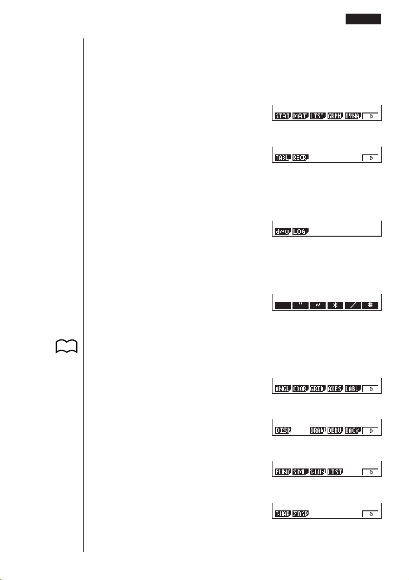
317
uu
uu
uTo change modes in a program
• Pressing 4 (MENU) while the program input screen is on the display causes a
mode change menu to appear. You can use this menu to input mode changes into
your programs. For details on each of these modes, see “To select an icon”, as
well as the sections of this manual that describe what you can do in each mode.
4(MENU)
6(g)
• The following menu appears whenever you press 4 (MENU) while inputting a
program that involves number base specifications.
4(MENU)
• Pressing 6 (SYBL) displays a menu of symbols that can be input into a pro-
gram.
6(SYBL)
• Pressing ! Z displays a menu of commands that can be used to change set
up screen settings inside a program. For details on each of these commands,
see “To change a mode set up”.
!Z
6(g)
6(g)
6(g)
123456
123456
123456
123456
123456
123456
123456
123456
P.5
Programming Examples 19 - 2

318
The following function key menu appears if you press !Z while inputting a
program that contains binary, octal, decimal, or hexadecimal calculation.
!Z
Actual program contents are identical to manual calculations. The following shows
how the calculation of the surface area and volume of a regular octahedron would be
calculated using a manual calculation.
Surface Area S .. c*!9d* <value of A> xw
Volume V ........... !9c/d* <value of A> Mdw
You could also perform this calculation by assigning the value for the length of one
side to variable A.
Length of One Side A
............ <value of A> aaAw
Surface Area S .. c*!9d*aAxw
Volume V ........... !9c/d*aAMdw
If you simply input the manual calculations shown above however, the calculator
would execute them from beginning to end, without stopping. The following com-
mands make it possible to interrupt a calculation for input of values and display of
intermediate results.
?:This command pauses program execution and displays a question mark as a
prompt for input of a value to assign to a variable. The syntax for this command
is: ? → <variable name>.
^^
^^
^: This command pauses program execution and displays the last calculation re-
sult obtained or text. It is similar to pressing w in a manual calculation.
• For full details on using these and other commands, see “Useful Program Com-
mands”.
The following shows examples of how to actually use the ? and ^ commands.
!W4(?)aaA6(g)5(:)
c*!9d*aAx
6(g)5(^)
!9c/d*aAMd
!Q or JJ
P.333
123456
19 - 2 Programming Examples
123456

319
uu
uu
uTo run a program
1. While the program list is on the display, use f and c to highlight the name of
the program you want to run.
2. Press 1 (EXE) or w to run the program.
Let’s try running the program we input above.
Length of One Side (A) Surface Area (S) Volume (V)
7 cm 169.7409791 cm
2
161.6917506 cm
3
10 cm 346.4101615 cm
2
471.4045208 cm
3
15 cm 779.4228634 cm
2
1590.990258 cm
3
1 (EXE) or w
hw
(Value of A)
Intermediate result produced by
^
w
w
baw
1 23456
Programming Examples 19 - 2

320
w
• Pressing w while the program’s final result is on the display re-executes the
program.
• You can also run a program while in the RUN Mode by inputting:
Prog ”<file name>” w.
• An error (Go ERROR) occurs if the program specified by Prog ”<file name>”
cannot be found.
19 - 2 Programming Examples
P.334

321
19-3 Debugging a Program
A problem in a program that keeps the program from running correctly is called a
“bug,” and the process of eliminating such problems is called “debugging.” Either of
the following symptoms indicates that your program contains bugs and that debug-
ging is required.
• Error messages appearing when the program is run
• Results that are not within your expectations
uu
uu
uTo eliminate bugs that cause error messages
An error message, like the one shown below, appears whenever something illegal
occurs during program execution.
When such a message appears, press d or e to display the location where the
error was generated, along with the cursor. Check the “Error Message Table” for
steps you should take to correct the situation.
• Note that pressing d or e will not display the location of the error if the pro-
gram is password protected.
uu
uu
uTo eliminate bugs that cause bad results
If your program produces results that are not what you normally expect, check the
contents of the program and make necessary changes. See “Editing File Names
and Program Contents” for details on how to change program contents.
P.399
P.323
P.328

322
19-4 Calculating the Number of Bytes Used by a
Program
This unit comes with 26 kbytes of memory. A byte is a unit of memory that can be
used for storage of data.
There are two types of commands: 1-byte commands and 2-byte commands.
• Examples of 1-byte commands: sin, cos, tan, log, (, ), A, B, C, 1, 2, etc.
• Examples of 2-byte commands: Lbl 1, Goto 2, etc.
While the cursor is located inside of a program, each press of d or e causes the
cursor to move one byte.
• You can check how much memory has been used and how much remains at any
time by selecting the MEM icon in the Main Menu and entering the MEM Mode.
See “Memory Status (MEM)” for details.
P.28

323
19-5 Secret Function
When inputting a program, you can protect it with a password that limits access to
the program contents to those who know the password. Password protected pro-
grams can be executed by anyone without inputting the password.
uu
uu
u To register a password
Example To create a program file under the name AREA and protect it with
the password CASIO
1. While the program list is on the display, press 3 (NEW) and input the file name
of the new program file.
3(NEW)
AREA
2. Press 5 (Q) and then input the password.
5(Q)
CASIO
• The password input procedure is identical to that used for file name input.
3. Press w to register the file name and password. Now you can input the contents
of the program file.
• Registration of a password uses 16 bytes of memory.
• Pressing w without inputting a password registers the file name only, without a
password.
4. After inputting the program, press ! Q to exit the program file and return to
the program list. Files that are password protected are indicated by an asterisk to
the right of the file name.
!Q
123456
P.315

324
uu
uu
uTo recall a program
Example To recall the file named AREA which is protected by the
password CASIO
1. In the program list, use f and c to move the highlighting to the name of the
program you want to recall.
2. Press 2 (EDIT).
2(EDIT)
3. Input the password and press w to recall the program.
• The message “Mismatch” appears if you input the wrong password.
19 - 5 Secret Function

325
19-6 Searching for a File
You can search for a specific file name using any of the three following methods.
• Scroll Search — scroll through the file names in the program list.
• File Name Search — input the name of the file.
• Initial Character Search — input the first few letters of the name of the file.
uu
uu
uTo find a file using scroll search
Example To use scroll search to recall the program named OCTA
1. While the program list is on the display, use f and c to scroll through the list
of program names until you find the one you want.
2. When the highlighting is located at the name of the file you want, press 2 (EDIT)
to recall it.
2(EDIT)
uu
uu
uTo find a file using file name search
Example To use file name search to recall the program named OCTA
1. While the program list is on the display, press 3 (NEW) and input the name of
the file you want to find.
• If the file you are looking for is password protected, you should also input the
password.
3(NEW)
OCTA
2. Press w to recall the program.
• If there is no program whose file name matches the one you input, a new file is
created using the input name.
1 2 3456
P.323

326
uu
uu
uTo find a file using initial character search
Example To use initial character search to recall the program named OCTA
1. While the program list is on the display, press 6 (g) 1 (SRC) and input the
initial characters of the file you want to find.
6(g)1(SRC)
OCT
2. Press w to search.
w
• All files whose file names start with the characters you input are recalled.
• If there is no program whose file name starts with the characters you input, the
message “Not Found” appears on the display. If this happens, press J to clear
the error message.
3. Use f and c to highlight the file name of the program you want to recall and
then press 2 (EDIT) to recall it.
19 - 6 Searching for a File

327
19-7 Searching for Data Inside a Program
Example To search for the letter “A” inside the program named OCTA
1. Recall the program, press 3 (SRC), and input the data you want to search for.
3(SRC)
aA
• You cannot specify the newline symbol (_ ) or display command (^) for the search
data.
2. Press w to begin the search. The contents of the program appears on the screen
with the cursor located at the first instance of the data you specified.
w
Indicates search operation is in progress
3. Press w to find the next instance of the data.
• If there is no match inside the program for the data you specified, the contents of
the program appear with the cursor located at the point from which you started
your search.
• Once the contents of the program are on the screen, you can use the cursor keys
(f, c, d, e) to move the cursor to another location before searching for
the next instance of the data. Only the part of the program starting from the
current cursor location is searched when you press w.
• Once the search finds an instance of your data, inputting characters or moving
the cursor causes the search operation to be cancelled (clearing the Search indi-
cator from the display).
• If you make a mistake while inputting characters to search for, press A to clear
your input and re-input from the beginning.
123456

328
19-8 Editing File Names and Program Contents
uu
uu
uTo edit a file name
Example To change the name of a file from TRIANGLE to ANGLE
1. While the program list is on the display, use f and c to move the highlighting
to the file whose name you want to edit and then press 6 (g) 2 (REN).
6(g)2(REN)
2. Make any changes you want.
DDD
3. Press w to register the new name and return to the program list.
• If the modifications you make result in a file name that is identical to the name of
a program already stored in memory, the message “Already Exists” appears.
When this happens, you can perform either of the following two operations to
correct the situation.
• Press e or d to clear the error and return to the file name input screen.
• Press A to clear the new file name and input a new one.
uu
uu
uTo edit program contents
1. Find the file name of the program you want in the program list.
2. Recall the program.
• The procedures you use for editing program contents are identical to those used
for editing manual calculations. For details, see “Editing Calculations”.
• The following function keys are also useful when editing program contents.
1 (TOP) ....... Moves the cursor to the top of the program
2 (BTM)....... Moves the cursor to the bottom of the program
P.23

329
Example 2 To use the OCTA program to create a program that calculates
the surface area and volume of regular tetrahedrons when the
length of one side is known
Use TETRA as the file name.
Length of One Side (A) Surface Area (S) Volume (V)
7 cm cm
2
cm
3
10 cm cm
2
cm
3
15 cm cm
2
cm
3
The following are the formulas used for calculating surface area S and volume V of a
regular tetrahedron for which the length of one side is known.
2
S = 3 A
2
, V = –––– A
3
12
Use the following key operations when inputting the program.
Length of One Side A ..!W4(?)aaA6(g)5(:)
Surface Area S ............!9d* aAx6(g)5(^)
Volume V .....................!9c/bc* aAMd
Compare this with the program for calculating the surface area and volume of a
regular octahedron.
Length of One Side A ..!W4(?)aaA6(g)5(:)
Surface Area S ............c*!9d*aAx6(g)5(^)
Volume V .....................!9c/d* aAMd
As you can see, you can produce the TETRA program by making the following changes
in the OCTA program.
• Deleting c * (underlined using a wavy line above)
• Changing d to b c (underlined using a solid line above)
Let’s edit OCTA to produce the TETRA program.
1. Edit the program name.
6(g)2(REN)TETRA
A
123456
Editing File Names and Program Contents 19 - 8

330
w
2. Edit the program contents.
2(EDIT)
eeeeDD
cd
331
w
baw
w
Editing File Names and Program Contents 19 - 8

332
19-9 Deleting a Program
There are two different ways to delete a file name and its program.
• Specific program delete
• All program delete
uu
uu
uTo delete a specific program
1. While the program list is on the display, use f and c to move the highlighting
to the name of the program you want to delete.
2. Press 4 (DEL).
4(DEL)
3. Press 1 (YES) to delete the selected program or 6 (NO) to abort the opera-
tion without deleting anything.
uu
uu
uTo delete all programs
1. While the program list is on the display, press 5 (DEL•A).
5(DEL•A)
2. Press 1 (YES) to delete all the programs in the list or 6 (NO) to abort the
operation without deleting anything.
• You can also delete all programs using the MEM Mode. See “Clearing Memory
Contents” for details.
1 23456
123456
P.30

333
19-10 Useful Program Commands
In addition to calculation commands, this calculator also includes a variety of rela-
tional and jump commands that can be used to create programs that make repeat
calculations quick and easy.
Program Menu
Press ! W to display the program menu.
!W
1 (COM)...... Program command menu
2 (CTL)........ Control command menu
3 (JUMP)..... Jump command menu
4 (?) ............ Input command
5 (^)........... Output command
6 (g) ........... Next menu
6(g)
1 (CLR) ....... Clear command menu
2 (DISP) ...... Display command menu
3 (REL) ....... Conditional jump relational operator menu
4 (I/O).......... Input/output command menu
5 (:) ............. Multi-statement command
6 (g) ........... Previous menu
Program Command Menu (COM)
While the program menu is on the display, press 1 (COM) to display the program
command menu.
1(COM)
1 (If) ............ If command
2 (Then) ...... Then command
3 (Else) ....... Else command
4 (I•End)...... IfEnd command
6 (g) ........... Next menu
123456
123456
123456

334
6(g)
1 (For) ......... For command
2 (To)........... To command
3 (Step) ....... Step command
4 (Next) ....... Next command
6 (g) ........... Next menu
6(g)
1 (Whle) ...... While command
2 (WEnd)..... WhileEnd command
3 (Do).......... Do command
4 (Lp•W)...... LpWhile command
6 (g) ........... Previous menu
Control Command Menu (CTL)
While the program menu is on the display, press 2 (CTL) to display the control
command menu.
2(CTL)
1 (Prog)....... Prog command
2 (Rtrn) ....... Return command
3 (Brk) ......... Break command
4 (Stop) ....... Stop command
Jump Command Menu (JUMP)
While the program menu is on the display, press 3 (JUMP) to display the jump
command menu.
3(JUMP)
1 (Lbl).......... Lbl command
2 (Goto)....... Goto command
3 (⇒) ........... ⇒ (jump) command
4 (Isz).......... Isz command
5 (Dsz) ........ Dsz command
123456
123456
123456
123456
19
-
10 Useful Program Commands

335
Clear Command Menu (CLR)
While the program menu is on the display, press 6 (g ) 1 (CLR) to display the
clear command menu.
6(g)1(CLR)
1 (Text) ........ ClrText command
2 (Grph) ...... ClrGraph command
3 (List)......... ClrList command
Display Command Menu (DISP)
While the program menu is on the display, press 6 (g) 2 (DISP) to display the
display command menu.
6(g)2(DISP)
1 (Stat) ........ DrawStat command
2 (Grph) ...... DrawGraph command
3 (Dyna)...... DrawDyna command
4 (F•Tbl)...... Table & Graph command menu
5 (R•Tbl)...... Recursion calculation and recursion formula graph command
menu
Pressing 4 (F•Tbl) while the display command menu is on the display causes the
Table & Graph command menu to appear.
4(F•Tbl)
1 (Tabl) ........ DispF-Tbl command
2 (G•Con).... DrawFTG-Con command
3 (G•Plt) ...... DrawFTG-Plt command
123456
123456
123456
Useful Program Commands 19
-
10

336
Pressing 5 (R•Tbl) while the display command menu is on the display causes the
recursion calculation and recursion formula graph command menu to appear.
5(R•Tbl)
1 (Tabl) ........ DispR-Tbl command
2 (Web) ....... DrawWeb command
3 (an•Cn)..... DrawR-Con command
4 (Σa•Cn) .... DrawRΣ-Con command
5 (an•Pl)...... DrawR-Plt command
6 (Σa•Pl)...... DrawRΣ-Plt command
Conditional Jump Relational Operator Menu (REL)
While the program menu is on the display, press 6 (g) 3 (REL) to display the
conditional jump relational operator menu.
6(g)3(REL)
1 (=) ............ Relational operator =
2 (
GG
GG
G
) ............ Relational operator
GG
GG
G
3 (>) ............ Relational operator >
4 (<) ............ Relational operator <
5 (≥) ............ Relational operator ≥
6 (≤) ............ Relational operator ≤
Input/Output Commands Menu (I/O)
While the program menu is on the display, press 6 (g) 4 (I/O) to display the
input/output command menu.
6(g)4(I/O)
1 (Lcte)........ Locate command
2 (Gtky) ....... Getkey command
3 (Send)...... Send ( command
4 (Recv) ...... Receive ( command
• The appearance of the function menu differs slightly for a program that contains
binary, octal, decimal, or hexadecimal calculation, but the functions in the menu
are the same.
123456
123456
123456
19
-
10 Useful Program Commands

337
19-11 Command Reference
kk
kk
k Command Index
Break..................................................................................... 343
ClrGraph................................................................................ 347
ClrList .................................................................................... 347
ClrText ................................................................................... 347
DispF-Tbl, DispR-Tbl............................................................. 347
Do~LpWhile........................................................................... 342
DrawDyna.............................................................................. 348
DrawFTG-Con, DrawFTG-Plt ................................................ 348
DrawGraph ............................................................................ 348
DrawR-Con, DrawR-Plt ......................................................... 348
DrawRΣ-Con, DrawRΣ-Plt ..................................................... 349
DrawStat................................................................................ 349
DrawWeb............................................................................... 349
Dsz ........................................................................................ 345
For~To~Next .......................................................................... 341
For~To~Step~Next ................................................................ 341
Getkey ................................................................................... 350
Goto~Lbl................................................................................ 345
If~Then.................................................................................. 339
If~Then~Else......................................................................... 340
If~Then~Else~IfEnd .............................................................. 340
If~Then~IfEnd ....................................................................... 339
Isz.......................................................................................... 346
Locate ................................................................................... 350
Prog....................................................................................... 343
Receive ( ............................................................................... 351
Return ................................................................................... 344
Send (.................................................................................... 351
Stop....................................................................................... 344
While~WhileEnd.................................................................... 342
? (Input Command) ............................................................... 338
^ (Output Command)........................................................... 338
: (Multi-statement Command)................................................ 338
_ (Carriage Return) ............................................................. 339
⇒ (Jump Code) ..................................................................... 346
=,
GG
GG
G
, >, <, ≥, ≤ (Relational Operators) ................................... 352

338
The following are conventions that are used in this section when describing the vari-
ous commands.
Boldface Text ............. Actual commands and other items that always must be in-
put are shown in boldface.
{Curly Brackets} ......... Curly brackets are used to enclose a number of items, one
of which must be selected when using a command. Do not
input the curly brackets when inputting a command.
[Square Brackets] ...... Square brackets are used to enclose items that are op-
tional. Do not input the square brackets when inputting a
command.
Numeric Expressions. Numeric expressions (such as 10, 10 + 20, A) indicate con-
stants, calculations, numeric constants, etc.
Alpha Characters ....... Alpha characters indicate literal strings (such as AB).
kk
kk
k Basic Operation Commands
? (Input Command)
Function: Prompts for input of values for assignment to variables during program
execution.
Syntax: ? → <variable name>
Example: ? → A _
Description:
1. This command momentarily interrupts program execution and prompts for input
of a value or expression for assignment to a variable. When the input command is
executed, “?” to appears on the display and the calculator stands by for input.
2. Input in response to the input command must be a value or an expression, and
the expression cannot be a multi-statement.
^^
^^
^ (Output Command)
Function: Displays and intermediate result during program execution.
Description:
1. This command momentarily interrupts program execution and displays alpha
character text or the result of the calculation immediately before it.
2. The output command should be used at locations where you would normally
press the w key during a manual calculation.
: (Multi-statement Command)
Function: Connects two statements for sequential execution without stopping.
Description:
1. Unlike the output command (^ ), statements connected with the multi-statement
command are executed non-stop.
2. The multi-statement command can be used to link two calculation expressions or
two commands.
19
-
11 Command Reference

339
3. You can also use a carriage return indicated by _ in place of the multi-statement
command.
__
__
_ (Carriage Return)
Function: Connects two statements for sequential execution without stopping.
Description:
1. Operation of the carriage return is identical to that of the multi-statement com-
mand.
2. Using a carriage return in place of the multi-statement command makes the dis-
played program easier to read.
kk
kk
k Program Commands (COM)
If~Then
Function: The Then-statement is executed only when the If-condition is true (non-
zero).
Syntax:
Parameters: condition, numeric expression
Description:
1. The Then-statement is executed only when the condition is true (non-zero).
2. If the condition is false (0), the Then-statement is not executed.
3. An If-condition must always be accompanied by a Then-statement. Omitting the
Then-statement results in an error (Syn ERROR).
Example: If A = 0 _
Then ”A = 0”
If~Then~IfEnd
Function: The Then-statement is executed only when the If-condition is true (non-
zero). The IfEnd-statement is always executed: after the Then-statement is executed
or directly after the If-condition when the If-condition is false (0).
Syntax:
Parameters: condition, numeric expression
__
If
<condition> : Then <statement> : <statement>
numeric expression
^^
If <condition>
_
:
^
Then <statement>
numeric expression
_
:
^
<statement>
_
:
^
IfEnd
Command Reference 19
-
11

340
19
-
11 Command Reference
Description:
This command is almost identical to If~Then. The only difference is that the IfEnd-
statement is always executed, regardless of whether the If-condition is true (non-
zero) or false (0).
Example: If A = 0 _
Then ”A = 0” _
IfEnd _
”END”
If~Then~Else
Function: The Then-statement is executed only when the If-condition is true (non-
zero). The Else-statement is executed when the If-condition is false (0).
Syntax:
Parameters: condition, numeric expression
Description:
1. The Then-statement is executed when the If-conditions is true (non-zero).
2. The Else-statement is executed when the If-conditions is false (zero).
Example: If A = 0 _
Then ”TRUE” _
Else ”FALSE”
If~Then~Else~IfEnd
Function: The Then-statement is executed only when the If-condition is true (non-
zero). The Else-statement is executed when the If-condition is false (0). The IfEnd-
statement is always executed following either the Then-statement or Else-statement.
Syntax:
Parameters: condition, numeric expression
Description:
This command is almost identical to If~Then~Else. The only difference is that the
IfEnd-statement is always executed, regardless of whether the If-condition is true
(non-zero) or false (0).
If
<condition>
_
:
^
Then <statement>
_
:
^
<statement>
numeric expression
_
:
^
Else <statement>
_
:
^
<statement>
If <condition>
_
:
^
Then <statement>
_
:
^
<statement>
numeric expression
_
:
^
Else <statement>
_
:
^
<statement>
_
:
^
IfEnd

341
Example: Lbl 1:? → A _
If A > 0 And A < 10 _
Then ”GOOD”_
Else Goto 1_
IfEnd
The above program displays the message “GOOD” whenever a value that is greater
than zero and less than 10 is input. Any other value prompts for input again.
For~To~Next
Function: This command repeats everything between the For-statement and the
Next-statement. The starting value is assigned to the control variable with the first
execution, and the value of the control variable is incremented by one with each
execution. Execution continues until the value of the control variable exceeds the
ending value.
Syntax:
Parameters:
• control variable name: A to Z
• starting value: value or expression that produces a value (i.e. sin
x, A, etc.)
• ending value: value or expression that produces a value (i.e. sin x, A, etc.)
Description:
1. When the starting value of the control variable is greater than the ending value,
execution continues from the statement following Next, without executing the
statements between For and Next.
2. A For-statement must always have a corresponding Next-statement, and the Next-
statement must always come after its corresponding For-statement.
3. The Next-statement defines the end of the loop created by For~Next, and so it
must always be included. Failure to do so results in an error (Go ERROR).
Example: For 1 → A To 10_
A × 3 → B_
B ^
Next
For~To~Step~Next
Function: This command repeats everything between the For-statement and the
Next-statement. The starting value is assigned to the control variable with the first
execution, and the value of the control variable is changed according to the step
value with each execution. Execution continues until the value of the control variable
exceeds the ending value.
_
For
<starting value> → <control variable name>
To
<ending value>
:
^
_
<statement>
: Next
^
Command Reference 19
-
11

342
Syntax:
Parameters:
• control variable name: A to Z
• starting value: value or expression that produces a value (i.e. sin
x, A, etc.)
• ending value: value or expression that produces a value (i.e. sin x, A, etc.)
• step value: numeric value (omitting this value sets the step to 1)
Description:
1. This command is basically identical to For~To~Next. The only difference is that
you can specify the step.
2. Omitting the step value automatically sets the step to 1.
3. Making the starting value less than the ending value and specifying a positive
step value causes the control variable to be incremented with each execution.
Making the starting value greater than the ending value and specifying a negative
step value causes the control variable to be decremented with each execution.
Example: For 1 → A To 10 Step 0.1_
A × 3 → B _
B ^
Next
Do~LpWhile
Function: This command repeats specific commands as long as its condition is true
(non-zero).
Syntax:
Parameters: expression
Description:
1. This command repeats the commands contained in the loop as long as its condi-
tion is true (non-zero). When the condition becomes false (0), execution pro-
ceeds from the statement following the LpWhile-statement.
2. Since the condition comes after the LpWhile-statement, the condition is tested
(checked) after all of the commands inside the loop are executed.
Example: Do_
? → A_
A × 2 → B_
B ^
LpWhile B >10
While~WhileEnd
Function: This command repeats specific commands as long as its condition is true
(non-zero).
_
For
<starting value> → <control variable name>
To
<ending value>
Step
<step value>
:
^
Next
_
Do
: ~ LpWhile <expression>
^
19
-
11 Command Reference

343
Syntax:
Parameters: expression
Description:
1. This command repeats the commands contained in the loop as long as its condi-
tion is true (non-zero). When the condition becomes false (0), execution pro-
ceeds from the statement following the WhileEnd-statement.
2. Since the condition comes after the While-statement, the condition is tested
(checked) before the commands inside the loop are executed.
Example: 10 → A_
While A > 0_
A – 1 → A_
”GOOD”_
WhileEnd
kk
kk
k Program Control Commands (CTL)
Break
Function: This command breaks execution of a loop and continues from the next
command following the loop.
Syntax: Break _
Description:
1. This command breaks execution of a loop and continues from the next command
following the loop.
2. This command can be used to break execution of a For-statement, Do-state-
ment, and While-statement.
Example: While A>0_
If A > 2_
Then Break_
IfEnd_
WhileEnd_
A ^ ← Executed after Break
Prog
Function: This command specifies execution of another program as a subroutine. In
the RUN Mode, this command executes a new program.
Syntax: Prog ”file name” _
Example: Prog ”ABC” _
Description:
1. Even when this command is located inside of a loop, its execution immediately
breaks the loop and launches the subroutine.
2. This command can be used as many times as necessary inside of a main routine
to call up independent subroutines to perform specific tasks.
_
While <expression>
: ~ WhileEnd
^
Command Reference 19
-
11

344
3. A subroutine can be used in multiple locations in the same main routine, or it can
be called up by any number of main routines.
D
CEIJ
Prog ”E” Prog ”I” Prog ”J”
A
Prog ”D”
Prog ”C”
4. Calling up a subroutine causes it to be executed from the beginning. After execu-
tion of the subroutine is complete, execution returns to the main routine, continu-
ing from the statement following the Prog command.
5. A Goto~Lbl command inside of a subroutine is valid inside of that subroutine only.
It cannot be used to jump to a label outside of the subroutine.
6. If a subroutine with the file name specified by the Prog command does not exist,
an error (Go ERROR) occurs.
7. In the RUN Mode, inputting the Prog command and pressing w launches the
program specified by the command.
Return
Function: This command returns from a subroutine.
Syntax: Return _
Description:
Execution of the Return command inside a main routine causes execution of the
program to stop.
Example: Prog ”A” Prog ”B”
1 → A_ For A → B To 10_
Prog ”B”_ B + 1 → C_
C ^ Next_
Return
Executing the program in File A displays the result of the operation (11).
Stop
Function: This command terminates execution of a program.
Syntax: Stop _
Description:
1. This command terminates program execution.
2. Execution of this command inside of a loop terminates program execution with-
out an error being generated.
Level 1 Level 2 Level 3 Level 4
Main Routine Subroutines
19
-
11 Command Reference

345
Example: For 2 → I To 10_
If I = 5_
Then ”STOP” : Stop_
IfEnd_
Next
This program counts from 2 to 10. When the count reaches 5, however, it terminates
execution and displays the message “STOP.”
kk
kk
k Jump Commands (JUMP)
Dsz
Function: This command is a count jump that decrements the value of a control
variable by 1, and then jumps if the current value of the variable is zero.
Syntax:
Parameters:
Variable Name: A to Z,
r,
θ
[Example] Dsz B : Decrements the value assigned to variable B by 1.
Description:
This command decrements the value of a control variable by 1, and then tests (checks)
it. If the current value is non-zero, execution continues with the next statement. If the
current value is zero, execution jumps to the statement following the multi-statement
command (:), display command (^), or carriage return (_).
Example: 10 → A : 0 → C :
Lbl 1 : ? → B : B+C → C :
Dsz A : Goto 1 : C ÷ 10
This program prompts for input of 10 values, and then calculates the
average of the input values.
Goto~Lbl
Function: This command performs an unconditional jump to a specified location.
Syntax: Goto <value or variable> ~ Lbl <value or variable>
Parameters: Value (from 0 to 9), variable (A to Z, r,
θ
)
Description:
1. This command consists of two parts: Goto
n (where n is a value from 0 to 9) and
Lbl n (where n is the value specified for Goto). This command causes program
execution to jump to the Lbl-statement whose value matches that specified by
the Goto-statement.
2. This command can be used to loop back to the beginning of a program or to jump
to any location within the program.
Variable Value
GG
GG
G
0
_
Dsz <variable name> : <statement> : <statement>
^
Variable Value = 0
Command Reference 19
-
11

346
3. This command can be used in combination with conditional jumps and count
jumps.
4. If there is no Lbl-statement whose value matches that specified by the Goto-
statement, an error (Go ERROR) occurs.
Example: ? → A : ? → B : Lbl 1 :
? → X : A × X + B ^
Goto 1
This program calculates
y = AX + B for as many values for each variable that you
want to input. To quit execution of this program, press A.
Isz
Function: This command is a count jump that increments the value of a control
variable by 1, and then jumps if the current value of the variable is zero.
Syntax:
Parameters:
Variable Name: A to Z,
r,
θ
[Example] Isz A : Increments the value assigned to variable A by 1.
Description:
This command increments the value of a control variable by 1, and then tests (checks)
it. If the current value is non-zero, execution continues with the next statement. If the
current value is zero, execution jumps to the statement following the multi-statement
command (:), display command (^), or carriage return (_).
⇒ (Jump Code)
Function: This code is used to set up conditions for a conditional jump. The jump is
executed whenever the conditions are false.
Syntax:
Parameters:
left side/right side: variable (A to Z,
r,
θ
), numeric constant, variable expression (such
as: A × 2)
relational operator: =,
GG
GG
G
, >, <, ≥, ≤
Variable Value
GG
GG
G
0
_
Isz <variable name> : <statement>
: <statement>
^
Variable Value = 0
True
_
<left side> <relational operator> <right side> ⇒ <statement>
:
<statement>
^
False
19
-
11 Command Reference
P.352

347
Description:
1. The conditional jump compares the contents of two variables or the results of two
expressions, and a decision is made whether or not to execute the jump based
on the results of the comparison.
2. If the comparison returns a true result, execution continues with the statement
following the ⇒ command. If the comparison returns a false result, execution
jumps to the statements following the multi-statement command (:), display com-
mand (^), or carriage return (_).
Example: Lbl 1 : ? → A :
A > 0 ⇒
A ^
Goto 1
With this program, inputting a value of zero or greater calculates and displays the
square root of the input value. Inputting a value less than zero returns to the input
prompt without calculating anything.
kk
kk
k Clear Commands (CLR)
ClrGraph
Function: This command clears the graph screen.
Syntax: ClrGraph_
Description: This command clears the graph screen during program execution.
ClrList
Function: This command clears list data.
Syntax: ClrList_
Description: This command clears the contents of the currently selected list (List 1
to List 6) during program execution.
ClrText
Function: This command clears the text screen.
Syntax: ClrText_
Description: This command clears text from the screen during program execution.
kk
kk
k Display Commands (DISP)
DispF-Tbl, DispR-Tbl
Function: These commands display numeric tables.
Syntax:
DispF-Tbl_
DispR-Tbl_
Command Reference 19
-
11

348
Description:
1. These commands generate numeric tables during program execution in accord-
ance with conditions defined within the program.
2. DispF-Tbl generates a function table, while DispR-Tbl generates a recursion ta-
ble.
DrawDyna
Function: This command executes a Dynamic Graph draw operation.
Syntax: DrawDyna_
Description: This command performs a Dynamic Graph draw operation during
program execution in accordance with the drawing conditions defined within the
program.
DrawFTG-Con, DrawFTG-Plt
Function: These commands graph functions.
Syntax:
DrawFTG-Con_
DrawFTG-Plt_
Description:
1. These commands graph functions in accordance with conditions defined within
the program.
2. DrawFTG-Con produces a connect type graph, while DrawFTG-Plt produces a
plot type graph.
DrawGraph
Function: This command draws a graph.
Syntax: DrawGraph_
Description: This command draws a graph in accordance with the drawing condi-
tions defined within the program.
DrawR-Con, DrawR-Plt
Function: These commands graph recursion expressions, with an(bn) as the vertical
axis and n as the horizontal axis.
Syntax:
DrawR-Con_
DrawR-Plt_
Description:
1. These commands graph recursion expressions, with
an(bn) as the vertical axis
and n as the horizontal axis, in accordance with conditions defined within the
program.
19
-
11 Command Reference

349
2. DrawR-Con produces a connect type graph, while DrawR-Plt produces a plot
type graph.
DrawRΣ-Con, DrawRΣ-Plt
Function: These commands graph recursion expressions, with Σan(Σbn) as the ver-
tical axis and n as the horizontal axis.
Syntax:
DrawRΣ-Con_
DrawRΣ-Plt_
Description:
1. These commands graph recursion expressions, with Σ
an(Σbn) as the vertical axis
and n as the horizontal axis, in accordance with conditions defined within the
program.
2. DrawRΣ-Con produces a connect type graph, while DrawRΣ-Plt produces a plot
type graph.
DrawStat
Function: This draws a statistical graph.
Syntax:
DrawStat_
Description:
This command draws a statistical graph in accordance with conditions defined within
the program.
DrawWeb
Function: This command graphs convergence/divergence of a recursion expres-
sion (WEB graph).
Syntax: DrawWeb [name of recursion expression], [number of lines]_
Example: DrawWeb
an+1 (bn+1), 5_
Description:
1. This command graphs convergence/divergence of a recursion expression (WEB
graph).
2. Omitting the number of lines specification automatically specifies the default value
30.
Command Reference 19
-
11

350
kk
kk
k Input/Output Commands (I/O)
Getkey
Function: This command returns the code that corresponds to the last key pressed.
Syntax: Getkey_
Description:
1. This command returns the code that corresponds to the last key pressed.
79
69 59 49 39 29
78 68 58 48
77 67 57 47
76 66 56 46 36
75 65 55 45 35
26
25
74
73
72
71
64
63
62
61
54
53
52
51
44
43
42
41
33
32
31
28
38
37
27
2. A value of zero is returned if no key was pressed previous to executing this com-
mand.
3. This command can be used inside of a loop.
Locate
Function: This command displays alpha-numeric characters at a specific location
on the text screen.
Syntax:
Locate <column number>, <line number>, <value>
Locate <column number>, <line number>, <variable name>
Locate <column number>, <line number>, ”<string>”
[Example] Locate 1, 1, ”AB”_
Parameters:
• line number: number from 1 to 7
• column number: number from 1 to 21
• value: numeric value
• variable name: A to Z
• string: character string
19
-
11 Command Reference

351
Description:
1. This command displays values (including variable contents) or text at a specific
location on the text screen.
2. The row is designated by a value from 1 to 7, which the column is designed by a
value from 1 to 21.
(1, 1) → ← (21, 1)
(1, 7) →←(21, 7)
Example: Cls_
Locate 7, 1, ”CASIO FX”
This program displays the text “CASIO FX” in the center of the screen.
• In some cases, the ClrText command should be executed before running the
above program.
Receive (
Function: This command receives data from an external device.
Syntax: Receive (<data>)
Description:
1. This command receives data from an external device.
2. The following types of data can be received by this command.
• Individual values assigned to variables
• Matrix data (all values - individual values cannot be specified)
• List data (all values - individual values cannot be specified)
• Picture data
Send (
Function: This command sends data to an external device.
Syntax: Send (<data>)
Description:
1. This command sends data to an external device.
2. The following types of data can be sent by this command.
• Individual values assigned to variables
• Matrix data (all values - individual values cannot be specified)
• List data (all values - individual values cannot be specified)
Command Reference 19
-
11

352
kk
kk
k Conditional Jump Relational Operators (REL)
=,
GG
GG
G
, >, <, ≥, ≤
Function: These relational operators are used in combination with the conditional
jump command.
Syntax:
Parameters:
left side/right side: variable (A to Z,
r,
θ
), numeric constant, variable expression (such
as: A × 2)
relational operator: =,
GG
GG
G
, >, <, ≥, ≤
Description:
1. The following six relational operators can be used in the conditional jump com-
mand
<left side> = <right side> : true when <left side> equals <right side>
<left side>
GG
GG
G
<right side> : true when <left side> does not equal <right side>
<left side> > <right side> : true when <left side> is greater than <right side>
<left side> < <right side> : true when <left side> is less than <right side>
<left side> ≥ <right side> : true when <left side> is greater than or equal to <right side>
<left side> ≤ <right side> : true when <left side> is less than or equal to <right side>
2. See “⇒ (Jump Code)” for details on using the conditional jump.
_
<left side> <relational operator> <right side> ⇒ <statement>
:
<statement>
^
P.346
19
-
11 Command Reference

353
19-12 Text Display
You can include text in a program by simply enclosing it between double quotation
marks. Such text appears on the display during program execution, which means
you can add labels to input prompts and results.
Program Display
? → X?
”X =” ? → X X = ?
• If the text is followed by a calculation formula, be sure to insert a display com-
mand (^) between the text and calculation.
• Inputting more than 21 characters causes the text to move down to the next line.
The screen scrolls automatically if the text causes the screen to become full.

354
19-13 Using Calculator Functions in Programs
kk
kk
k Using Matrix Row Operations in a Program
These commands let you manipulate the rows of a matrix in a program.
• For this type of program, be sure to use the MAT Mode to input the matrix, and
then switch to the PRGM Mode to input the program.
uu
uu
uTo swap the contents of two rows (Swap)
Example 1 To swap the values of Row 2 and Row 3 in the following matrix:
12
Matrix A =
34
56
The following is the syntax to use for this program.
Swap
A, 2, 3
Matrix name
Executing this program produces the following result.
(MAT Mode)
uu
uu
uTo calculate a scalar product (
``
``
` Row)
Example 2 To calculate the scalar product of Row 2 of the matrix in Example 1,
multiplying by 4
The following is the syntax to use for this program.
`Row
4, A, 2
Matrix name
Multiplier
Executing this program produces the following result.
(MAT Mode)
P.92

355
uu
uu
uTo calculate a scalar product and add the results to another row
(
``
``
`Row+)
Example 3 To calculate the scalar product of Row 2 of the matrix in Example 1,
multiplying by 4, and add the result to row 3
The following is the syntax to use for this program.
`Row+
4, A, 2, 3
Matrix name
Multiplier
Executing this program produces the following result.
(MAT Mode)
uu
uu
uTo add two rows (Row+)
Example 4 To add Row 2 to Row 3 of the matrix in Example 1
The following is the syntax to use for this program.
Row+ A, 2, 3
Matrix name
Executing this program produces the following result.
(MAT Mode)
kk
kk
k Using Graph Functions in a Program
You can incorporate graph functions into a program to draw complex graphs and to
overlay graphs on top of each other. The following shows various types of syntax you
need to use when programming with graph functions.
• View Window
View Window –5, 5, 1, –5, 5, 1 _
• Graph function input
Y = Type_ ..... Specifies graph type.
”X
2
– 3” → Y1_
• Graph draw operation
DrawGraph_
Example Program
1
ClrGraph_
1
!W612
2
View Window –10, 10, 2, –120, 150, 50_
2
!31J
3
Y = Type_
3
4431
”X ^ 4–X ^ 3–24X
2
+ 4X + 80” → Y1_
4
J41JJ
P.126
Using Calculator Functions in Programs 19
-
13
4

356
5
G SelOn 1_
5
4411J
6
DrawGraph
6
!W622
Executing this program produces the result shown here.
kk
kk
k Using Dynamic Graph Functions in a Program
Using Dynamic Graph functions in a program makes it possible to perform repeat
Dynamic Graph operations. The following shows how to specify the Dynamic Graph
range inside a program.
• Dynamic Graph range
1 → D Start_
5 → D End_
1 → D pitch_
Example Program
ClrGraph_
View Window –5, 5, 1, –5, 5, 1_
Y = Type_
”AX + 1” →
Y1_
1
J41JJ
2
D SelOn 1_
2
451
3
D Var A_
3
3
1 →
4
D Start_
4
J51
5 →
5
D End_
5
2
1 →
6
D pitch_
6
3
7
DrawDyna
7
!W623
Executing this program produces the result shown here.
↑
↓
19
-
13 Using Calculator Functions in Programs
P.208
1

357
kk
kk
k Using Table & Graph Functions in a Program
Table & Graph functions in a program can generate numeric tables and perform
graphing operations. The following shows various types of syntax you need to use
when programming with Table & Graph functions.
• Table range setting
1 → F Start_
5 → F End_
1 → F pitch_
• Numeric table generation
DispF-Tbl_
• Graph draw operation
Connect type: DrawFTG-Con_
Plot type: DrawFTG-Plt_
Example Program
ClrGraph_
ClrText_
View Window 0, 6, 1, –2, 106, 2_
Y = Type_
”3X
2
– 2” → Y1_
1
T SelOn 1_
1
4611
0 →
2
F Start_
2
J611
6 →
3
F End_
3
2
1 →
4
F pitch_
4
3
5
DispF-Tbl^
5
!W6241
6
DrawFTG-Con
6
!W6242
Executing this program produces the results shown here.
Numeric Table
Graph
w
P.236
Using Calculator Functions in Programs 19
-
13

358
kk
kk
k Using Recursion Table & Graph Functions in a Program
Incorporating Recursion Table & Graph functions in a program lets you generate
numeric tables and perform graphing operations. The following shows various types
of syntax you need to use when programming with Recursion Table & Graph func-
tions.
• Recursion formula input
an+1 Type_ .... Specifies recursion type.
”3an + 2” → an+1_
”4
bn + 6” → bn+1_
• Table range setting
1 → R Start_
5 → R End_
1 →
a0_
2 → b0_
1 → an Start_
3 →
bn Start_
• Numeric table generation
DispR-Tbl_
• Graph draw operation
Connect type: DrawR-Con_, DrawRΣ-Con_
Plot type: DrawR-Plt_, DrawRΣ-Plt_
• Statistical convergence/divergence graph (WEB graph)
DrawWeb
an+1, 10_
Example Program
ClrGraph_
View Window 0, 1, 1, 0, 1, 1_
1
an+1 Type_
1
46232J
”–3
an
2
+ 3an” → an+1_
2
42
”3bn – 0.2” → bn+1_
0 →
3
R Start_
3
J6221
6 → R End_
0.01 →
a0_
0.11 → b0_
0.01 → an Start_
0.11 →
bn Start_
4
DispR-Tbl^
4
!W6251
5
DrawWeb an+1, 30
5
!W6252JJJ
6
46243
P.250
19
-
13 Using Calculator Functions in Programs
2
6

359
Executing this program produces the results shown here.
Numeric Table
w
Recursion graph
w
kk
kk
k Using List Sort Functions in a Program
These functions let you sort the data in lists into ascending or descending order.
• Ascending order
SortA (List 1, List 2, List 3)
Lists to be sorted (up to six can be specified)
1
431J
2
K11
• Descending order
SortD (List 1, List 2, List 3)
Lists to be sorted (up to six can be specified)
kk
kk
k Using Statistical Calculations and Graphs in a Program
Including statistical calculations and graphing operations into program lets you cal-
culate and graph statistical data.
uu
uu
uTo set conditions and draw a statistical graph
Following “StatGraph”, you must specify the following graph conditions:
• Graph draw/non-draw status (DrawOn/DrawOff)
• Graph Type
•
x-axis data location (list name)
• y-axis data location (list name)
• Frequency data location (list name)
• Mark Type
The graph conditions that are required depends on the graph type. See “Changing
Graph Parameters”.
P.265
P.284
Using Calculator Functions in Programs 19
-
13
12
P.286

360
• The following is a typical graph condition specification for a scatter diagram or
x,
y line graph.
S-Gph1 DrawOn, Scatter, List1, List2, 1, Square_
In the case of an x, y line graph, replace “Scatter” in the above specification with
“xyLine”.
• The following is a typical graph condition specification for a single-variable graph.
S-Gph1 DrawOn, Hist, List1, List2_
The same format can be used for the following types of graphs, by simply replac-
ing “Hist” in the above specification with the applicable graph type.
Histogram: ......................Hist
Median Box: ...................MedBox
Mean Box: ......................MeanBox
Normal Distribution:........N-Dist
Broken Line: ...................Broken
• The following is a typical graph condition specification for a regression graph.
S-Gph1 DrawOn, Linear, List1, List2, List3_
The same format can be used for the following types of graphs, by simply replac-
ing “Linear” in the above specification with the applicable graph type.
Linear Regression: .........Linear
Med-Med: .......................Med-Med
Quadratic Regression:....Quad
Cubic Regression: ..........Cubic
Quartic Regression : ...... Quart
Logarithmic Regression: .. Log
Exponential Regression: Exp
Power Regression : ........Power
Example Program
ClrGraph_
S-Wind Auto_
{1, 2, 3} → List 1_
{1, 2, 3} → List 2_
S-Gph1 DrawOn, Scatter, List1, List2, 1, Square_
DrawStat
Executing this program produces the scatter diagram shown here.
19
-
13 Using Calculator Functions in Programs
P.289
P.289
3
8
2
56 74
1
1
!Z6631
2
K11
3
1JJ
4
4121J
5
11J
6
24J
7
J41
8
!W621

361
kk
kk
k Performing Statistical Calculations
• Single-variable statistical calculation
1
1-Variable List1, List2
Frequency data (Frequency)
x
-axis data (XList)
1
4161
• Paired-variable statistical calculation
2-Variable List1, List2, List3
Frequency data (Frequency)
y
-axis data (YList)
x
-axis data (XList)
• Regression statistical calculation
1
LinearReg List1, List2, List3
Calculation Frequency data (Frequency)
type*
y
-axis data (YList)
x
-axis data (XList)
1
41661
* Any one of the following can be specified as the calculation type.
LinearReg....... linear regression
Med-MedLine . Med-Med calculation
QuadReg ........ quadratic regression
CubicReg ....... cubic regression
QuartReg ....... quartic regression
LogReg........... logarithmic regression
ExpReg .......... exponential regression
PowerReg....... power regression
Using Calculator Functions in Programs 19
-
13

Data Communications
This chapter tells you everything you need to know to transfer pro-
grams between the fx-9750G and certain CASIO Graphic Scientific
Calculator models connected with an optionally available SB-62
cable. To transfer data between a unit and a personal computer,
you will need to purchase the separately available CASIO FA-122
Interface Unit.
This chapter also contains information on how to use the optional
SB-62 cable to connect to a CASIO Label Printer to transfer screen
data for printing.
20-1 Connecting Two Units
20-2 Connecting the Unit with a Personal Computer
20-3 Connecting the Unit with a CASIO Label Printer
20-4 Before Performing a Data Communication Operation
20-5 Performing a Data Transfer Operation
20-6 Screen Send Function
20-7 Data Communications Precautions
Chapter
20

364
20-1 Connecting Two Units
The following procedure describes how to connect two units with an optional SB-62
connecting cable for transfer of programs between them.
uu
uu
uTo connect two units
1. Check to make sure that the power of both units is off.
2. Remove the covers from the connectors of the two units.
• Be sure you keep the connector covers in a safe place so you can replace them
after you finish your data communications.
3. Connect the two units using the SB-62 cable.
SB-62 cable
• Keep the connectors covered when you are not using them.

365
20-2 Connecting the Unit with a Personal
Computer
To transfer data between the unit and a personal computer, you must connect them
through a separately available CASIO FA-122 Interface Unit.
For details on operation, the types of computer that can be connected, and hardware
limitations, see the user’s manual that comes with the FA-122.
uu
uu
uTo connect the unit with a personal computer
1. Check to make sure that the power of the unit and the personal computer is off.
2. Connect the personal computer to the FA-122 Interface Unit.
3. Remove the cover from the connector of the unit.
• Be sure you keep the connector cover in a safe place so you can replace it after
you finish your data communications.
4. Connect the unit to the FA-122 Interface Unit.
5. Switch on the power of the unit, followed by the personal computer.
• After you finish data communications, switch off power in the sequence: the unit
first, and then the personal computer. Finally, disconnect the equipment.
fx-9750G

366
20-3 Connecting the Unit with a CASIO Label
Printer
After you connect the unit to a CASIO Label Printer with an optional SB-62 cable,
you can use the Label Printer to print screen shot data from the unit. See the User’s
Manual that comes with your Label Printer for details on how to perform this opera-
tion.
• The operation described above can be performed using the following Label Printer
models: KL-2000, KL-2700, KL-8200 (as of October 1996).
uu
uu
uTo connect the unit with a Label Printer
1. Check to make sure that the power of the unit and the Label Printer is off.
2. Connect the optional SB-62 cable to the Label Printer.
3. Remove the cover from the connector of the unit.
• Be sure you keep the connector cover in a safe place so you can replace it after
you finish your data communications.
4. Connect the other end of the SB-62 cable to the unit.
5. Switch on the power of the unit, followed by the Label Printer.
• After you finish data communications, switch off power in the sequence: the unit
first, and then the Label Printer. Finally, disconnect the equipment.
SB-62 cable
fx-9750G
Label Printer

367
20-4 Before Performing a Data Communication
Operation
In the Main Menu, select the LINK icon and enter the LINK Mode. The following data
communication main menu appears on the display.
Image Set:Off...... Indicates the status of the graphic image send features.
Off: Graphic images not sent.
On: Pressing M sends graphic images.
1 (TRAN)..... Menu of send settings
2 (RECV) .... Menu of receive settings
6 (IMGE) ..... Menu of graphic image transfer settings
Communications parameters are fixed at the following settings.
• Speed (BPS): 9600 bits per second
• Parity (PARITY): NONE
P.372
123456

368
20-5 Performing a Data Transfer Operation
Connect the two units and then perform the following procedures.
Receiving unit
To set up the calculator to receive data, press 2 (RECV) while the data communi-
cation main menu is displayed.
2(RECV)
The calculator enters a data receive standby mode and waits for data to arrive.
Actual data receive starts as soon as data is sent from the sending unit.
Sending unit
To set up the calculator to send data, press 1 (TRAN) while the data communica-
tion main menu is displayed.
1 (TRAN)
Press the function key that corresponds to the type of data you want to send.
1 (SEL)........ Selects data items and sends
2 (CRNT) .... Selects data items from among previously selected data items
and sends
6 (BACK)..... All memory contents, including mode settings
uu
uu
uTo send selected data items
Press 1 (SEL) or 2 (CRNT) to display a data item selection screen.
1(SEL) or 2(CRNT)
Data items
123456
123456

369
1 (SEL)........ Selects data item where cursor is located.
6 (TRAN)..... Sends selected data items.
Use the f and c cursor keys to move the cursor to the data item you want to
select and press 1 (SEL) to select it. Currently selected data items are marked
with “'”. Pressing 6 (TRAN) sends all the selected data items.
• To deselect a data item, move the cursor to it and press 1 (SEL) again.
Only items that contain data appear on the data item selection screen. If there are
too many data items to fit on a single screen, the list scrolls when you move the
cursor to the bottom line of the items on the screen.
The following are the types of data items that can be sent.
Data Item Contents
Overwrite Password
Check*
1
Check*
2
Program Program contents Yes Yes
Mat n Matrix memory (A to Z) contents Yes
List n List memory (1 to 6) contents Yes
File n List file memory (1 to 6) contents Yes
Y=Data
Graph expressions, graph write/
non-write status, View Window No
contents, zoom factors
G-Mem n Graph memory (1 to 6) contents Yes
V-Win n View Window memory contents No
Picture n Picture (graph) memory (1 to 6) data No
DynaMem Dynamic Graph functions Yes
Equation Equation calculation coefficient values No
Variable Variable assignments No
F-Mem Function memory (1 to 6) contents No
*
1
No overwrite check: If the receiving unit already contains the same type of data, the existing
data is overwritten with the new data.
With overwrite check: If the receiving unit already contains the same type of data, a mes-
sage appears to ask if the existing data should be overwritten with the new data.
Performing a Data Transfer Operation 20 - 5

370
1 (YES) ....... Replaces the receiving unit’s existing data with the new data.
6 (NO) ......... Skips to next data item.
*
2
With password check: If a file is password protected, a message appears asking
for input of the password.
Name of password protected file
Password input field
6 (SYBL) ..... Symbol input
After inputting the password, press w.
uu
uu
uTo execute a send operation
After selecting the data items to send, press 6 (TRAN). A message appears to
confirm that you want to execute the send operation.
6(TRAN)
1 (YES) ....... Sends data.
6 (NO) ......... Returns to data selection screen.
Press 1 (YES) to send the data.
1(YES)
• You can interrupt a data operation at any time by pressing A.
123456
123456
123456
20 - 5 Performing a Data Transfer Operation
Data item name

371
The following shows what the displays of the sending and receiving units look like
after the data communication operation is complete.
Sending Unit Receiving Unit
Press A to return to the data communication main menu.
uu
uu
uTo send backup data
This operation allows you to send all memory contents, including mode settings.
While the send data type selection menu is on the screen, press 6 (BACK), and
the back up send menu shown below appears.
6(BACK)
Press 6 (TRAN) to start the send operation.
6(TRAN)
The following shows what the displays of the sending and receiving units look like
after the data communication operation is complete.
Sending Unit Receiving Unit
Press A to return to the data communication main menu.
• Data can become corrupted, necessitating a RESET of the receiving unit, should
the connecting cable become disconnected during data transfer. Make sure
that the cable is securely connected to both units before performing any data
communication operation.
123456
Performing a Data Transfer Operation 20 - 5

372
20-6 Screen Send Function
The following procedure sends a bit mapped screen shot of the display to a con-
nected computer.
uu
uu
uTo send the screen
1. Connect the unit to a personal computer or to a CASIO Label Printer.
2. In the data communication main menu, press 6 (IMGE), and then select “On”
for Image Set.
6(IMGE)
1(OFF) ........ Graphic images not sent
2(ON) .......... Bit map
3. Display the screen you want to send.
4. Set up the personal computer or Label Printer to receive data. When the other
unit is ready to receive, press M to start the send operation.
You cannot send the following types of screens to a computer.
• The screen that appears while a data communication operation is in progress.
• A screen that appears while a calculation is in progress.
• The screen that appears following the reset operation.
• The low battery message.
• The flashing cursor is not included in the screen image that is sent from the
unit.
• If you send a screen shot of any of the screens that appear during the data
send operation, you will not be able to then use the sent screen to proceed with
the data send operation. You must exit the data send operation that produced
the screen you sent and restart the send operation before you can send addi-
tional data.
• You cannot use 6mm wide tape to print a screen shot of a graph.
P.365
P.366
123456

373
20-7 Data Communications Precautions
Note the following precautions whenever you perform data communications.
• A TRANSMIT ERROR occurs whenever you try to send data to a receiving unit
that is not yet standing by to receive data. When this happens, press A to clear
the error and try again, after setting up the receiving unit to receive data.
• A RECEIVE ERROR occurs whenever the receiving unit does not receive any
data approximately six minutes after it is set up to receive data. When this hap-
pens, press A to clear the error.
• A TRANSMIT ERROR or RECEIVE ERROR occurs during data communications
if the cable becomes disconnected, if the parameters of the two units do not
match, or if any other communications problem occurs. When this happens, press
A to clear the error and correct the problem before trying data communications
again. If data communications are interrupted by A key operation or an error,
any data successfully received up the interruption will be in the memory of the
receiving unit.
• A MEMORY FULL occurs if the receiving unit memory becomes full during data
communications. When this happens, press A to clear the error and delete
unneeded data from the receiving unit to make room for the new data, and then
try again.
• To send picture (graph) memory data, the receiving unit need 1-kbytes of memory
for use as a work area in addition to the data being received.

Program Library
1 Prime Factor Analysis
2 Greatest Common Measure
3 t-Test Value
4 Circle and Tangents
5 Rotating a Figure
Before using the Program Library
• Be sure to check how many bytes of unused memory is remain-
ing before attempting to perform any programming.
• This Program Library is divided into two sections: a numeric cal-
culation section and a graphics section. Programs in the numeric
calculation section produce results only, while graphics programs
use the entire display area for graphing. Also note that calcula-
tions within graphics programs do not use the multiplication sign
(×) wherever it can be dropped (i.e. in front of open parenthesis).
Chapter
21

376
PROGRAM SHEET
Program for
Prime Factor Analysis
Description
Produces prime factors of arbitrary positive integers
For 1 < m < 10
10
Prime numbers are produced from the lowest value first. “END” is displayed at the end
of the program.
(Overview)
m is divided by 2 and by all successive odd numbers (d = 3, 5, 7, 9, 11, 13, ....) to check
for divisibility.
Where d is a prime factor, mi = mi–1/d is assumed, and division is repeated until
mi + 1 < d.
Example [1]
119 = 7 × 17
[2]
440730 = 2 × 3 × 3 × 5 × 59 × 83
[3]
262701 = 3 × 3 × 17 × 17 × 101
Preparation and operation
• Store the program written on the next page.
• Execute the program as shown below.
Step Key operation Display Step Key operation Display
No.
1

377
1
2
3
4
5
6
7
8
9
10
11
12
13
14
15
16
17
18
19
20
21
22
23
24
25
26
27
P
Lbl
Lbl
Lbl
Lbl
Lbl
Goto
Lbl
Lbl
Lbl
Lbl
Lbl
R
0
1
2
3
4
6
5
6
7
8
9
M
:
:
:
:
:
:
:
:
:
:
:
"
2
Frac
B
B
A
B
A
"
F
M
^
(
A
I
+
÷
^
^
E
A
"
A
A
+
C
2
B
A
N
C
?
÷
÷
1
⇒
→
×
÷
D
T
→
2
2
→
Goto
B
B
B
"
:
A
=
:
:
Goto
A
A
Goto
A
→
)
C
8
:
–
→
^
Goto
:
0
Frac
4
=
:
0
2
A
⇒
(
:
0
Goto
:
=
Goto
A
⇒
3
1
1
÷
Goto
:
⇒
:
B
7
A
B
C
D
E
F
G
H
I
J
K
L
M
N
O
P
Q
R
S
T
U
V
W
X
Y
Z
mi
d
mi +1
Goto
3
)
:
9
→
=
Goto
:
B
0
5
:
⇒
:
No.
1
Line
Program
File
name
Memory Contents

378
PROGRAM SHEET
Program for
Greatest Common Measure
Description
Euclidean general division is used to determine the greatest common measure for two interers
a and b.
For |a|, |b| < 10
9
, positive values are taken as < 10
10
(Overview)
n0 = max (|a|, |b|)
n1 = min (|a|, |b|)
nk–2
nk = nk–2 – ––– nk–1
nk–1
k = 2, 3....
If nk = 0, then the greatest common measure (c) will be nk–1.
Example [1] [2] [3]
When a = 238 a = 23345 a = 522952
b = 374 b = 9135 b = 3208137866
↓↓ ↓
c = 34 c = 1015 c = 998
Preparation and operation
• Store the program written on the next page.
• Execute the program as shown below.
Step Key operation Display Step Key operation Display
No.
2

379
1
2
3
4
5
6
7
8
9
10
11
12
13
14
15
16
17
18
19
20
21
22
23
24
25
26
27
C
Lbl
Abs
B
A
Lbl
C
B
Lbl
M
1
A
<
→
2
=
→
3
N
:
→
A
C
:
0
A
:
"
A
⇒
:
(
–
)
⇒
:
B
F
A
:
Goto
B
(
Goto
C
^
A
"
Abs
2
→
lnt
3
→
Goto
C
?
B
:
A
(
:
B
1
T
→
→
:
A
:
:
:
→
B
2
A
B
C
÷
Goto
"
B
)
:
B
:
×
"
B
?
–
→
A
A
B
C
D
E
F
G
H
I
J
K
L
M
N
O
P
Q
R
S
T
U
V
W
X
Y
Z
a, n
0
b, n
1
n
k
B
)
:
→ C:
No.
2
Line
Program
File
name
Memory Contents

380
PROGRAM SHEET
t =
(x – m)
x n–1
n
Program for
t-Test Value
Description
The mean (sample mean) and sample standard deviation can be used to obtain a t-test value.
x : mean of x data
xσn–1 : sample standard deviation of x data
n : number of data items
m : hypothetical population standard deviation (normally repre-
sented by
µ
, but m is used here because of variable name
limitations)
Example To determine whether the population standard deviation for sample data 55, 54, 51,
55, 53, 53, 54, 52, is 53.
Perform a t-test with a level of significance of 5%.
Preparation and operation
• Store the program written on the next page.
• Execute the program as shown below.
No.
3
Step Key operation Display Step Key operation Display
The above operation produces a t-test value of t(53) = 0.7533708035. According to the t-distribution
table in the next page, a level of significance of 5% and a degree of freedom of 7 (n – 1 = 8 – 1 = 7)
produce a two-sided t-test value of approximately 2.365. Since the calculated t-test value is lower
than the table value, the hypothesis that population mean m equals 53 is accepted.

381
1
2
3
4
5
6
7
8
9
10
15
20
25
30
35
40
45
50
60
80
120
240
∞
0.2
3.078
1.886
1.638
1.533
1.476
1.440
1.415
1.397
1.383
1.372
1.341
1.325
1.316
1.310
1.306
1.303
1.301
1.299
1.296
1.292
1.289
1.285
1.282
0.1
6.314
2.920
2.353
2.132
2.015
1.943
1.895
1.860
1.833
1.812
1.753
1.725
1.708
1.697
1.690
1.684
1.679
1.676
1.671
1.664
1.658
1.651
1.645
12.706
4.303
3.182
2.776
2.571
2.447
2.365
2.306
2.262
2.228
2.131
2.086
2.060
2.042
2.030
2.021
2.014
2.009
2.000
1.990
1.980
1.970
1.960
63.657
9.925
5.841
4.604
4.032
3.707
3.499
3.355
3.250
3.169
2.947
2.845
2.787
2.750
2.724
2.704
2.690
2.678
2.660
2.639
2.617
2.596
2.576
0.05 0.01
1
2
3
4
5
6
7
T
{
5
l-Var
Lbl
(
"
Goto
5
4
List
0
x
T
0
T
5
,
1
:
–
=
E
,
5
,
"
M
"
S
5
2
1
M
)
:
T
4
}
_
"
÷
T
,
→
?
(
^
5
List
→
xσn–1
,
_
_
1
1
M
÷
5
n
5
)
,
→
5
T
3
_
A
B
C
D
E
F
G
H
I
J
K
L
M
N
O
P
Q
R
S
T
U
V
W
X
Y
Z
mt
,53,
P (Probability)
Degree
of Freedom
No.
3
Line
Program
• t-distribution table
The values in the top row of the table show the probability (two-sided
probability) that the absolute value of t is greater than the table values
for a given degree of freedom.
Memory Contents
File
name
M:aM
T:aT

382
PROGRAM SHEET
Program for
Circle and Tangents
Description
Formula for circle:
x
2
+ y
2
= r
2
Formula for tangent line passing
through point A (x', y'):
y – y' = m (x – x')
*
m represents the slope of the
tangent line
With this program, slope m and intercept b (= y' – mx') are obtained for lines drawn from point
A (x', y') and are tangent to a circle with a radius of r. The trace function is used to read out the
coordinates at the points of tangency, and factor zoom is used to enlarge the graph.
Example
To determine m and b for the following values:
r = 1
x'= 3
y'= 2
Notes
• The point plotted for A cannot be moved. Even if it is moved on the graph, the calculation is
performed using the original value.
• An error (Ma ERROR) occurs when r = x'.
• Be sure to always perform a trace operation whenever you select trace and the message
TRACE is on the display.
Preparation and operation
• Store the program written on the next page.
• Execute the program as shown below.
No.
4
0
X
Y
A
(x',y')
r
A
B
C
D
E
F
G
H
I
J
K
L
M
N
O
P
Q
R
S
T
U
V
W
X
Y
Z
Memory Contents

383
1
2
3
4
5
6
7
8
9
10
11
12
13
14
15
16
17
18
19
20
21
22
23
24
25
26
27
28
29
30
31
32
33
34
T
Prog
"
R
Prog
"
X
"
Plot
R
(
Lbl
Graph Y=
"
"
Lbl
"
Y
N
1
Z
Lbl
(
Graph Y=
"
"
Lbl
"
Y
N
2
Z
Lbl
"
"
A
"
X
=
"
(
=
Y
A
x
2
6
M
M
B
0
T
E
O
→
=
2
(–)
N
M
B
5
T
E
O
→
=
1
T
Factor
N
W
x
2
"
C
X
"
=
,
(
P
_
(
=
=
_
R
S
⇒
S
0
_
A
(
=
=
_
R
S
⇒
S
0
_
R
N
G
I
+
?
I
,
?
"
B
A
–
X
"
"
A
⇒
0
:
⇒
B
X
"
"
A
⇒
0
:
⇒
A
:
E
N
Y
→
R
Y
→
?
^
x
2
A
–
:
:
C
1
"
Z
Goto
–
–
:
:
C
1
"
Z
Goto
C
N
N
D
x
2
R
C
)
A
→
+
B
A
M
B
E
_
:
=
2
A
N
B
E
_
:
=
3
E
=
T
O
=
_
L
_
_
B
B
)
)
^
–
?
?
1
:
P
)
^
–
?
?
1
:
"
"
W
R
E
_
x
2
(
+
M
_
→
⇒
Goto
)
+
N
_
→
⇒
Goto
^
?
_
_
^
R
x
2
^
^
_
1
_
R
^
^
_
1
_
F
"
x
2
"
–
R
B
A
Z
Goto
0
(
B
A
Z
Goto
5
→
x
2
–
)
A
→
x
2
P
)
_
x
–1
_
_
:
x
2
–
Factor
A
F
x
2
_
)
→
x
–1
M
→
_
N
_
No.
4
Line
Program
File
name

384
View
Window
35
36
37
38
39
40
41
42
43
44
1
2
1
2
Prog
S
Graph Y=
Goto
Lbl
Graph Y=
Prog
:
Lbl
"
W
1
C
Graph Y=
Graph Y=
"
=
N
3
9
M
"
Goto
3
E
I
(–)
,
I
(–)
C
2
(
_
_
(
W
6
_
N
N
6
1
R
(
I
⇒
X
X
I
_
D
D
.
C
R
(
R
Graph Y=
–
–
N
"
O
3
L
x
2
R
C
M
A
A
D
W
,
E
–
x
2
L
(
)
)
O
6
X
–
E
X
+
+
W
.
x
2
X
:
A
^
^
:
,
_
)
"
–
B
B
"
3
)
x
2
S
)
Prog
1
=
+
"
,
1
B
C
(–)
⇒
_
I
3
Goto
R
.
9
C
1
_
L
,
E
3
"
.
No.
4
Line
Program
File
name
File
name

385
1
2
3
4
5
Program for
Circle and Tangents
No.
4
Step Key Operation Display

386
Program for
Circle and Tangents
No.
4
Step Key Operation Display
6
7
8
9
10

387
11
12
13
14
15
Program for
Circle and Tangents
No.
4
Step Key Operation Display

388
16
17
18
Program for
Circle and Tangents
No.
4
Step Key Operation Display

389
A
B
C
D
E
F
G
x
1
y
1
x
2
y
2
x
3
y
3
x'
1
y'
1
x'
2
y'
2
x'
3
y'
3
H
I
J
K
L
M
N
O
P
Q
R
S
T
U
V
W
X
Y
Z
0
X
Y
B(x
2,
y
2
)
A(x
1,
y
1
)
C(x
3,
y
3
)
PROGRAM SHEET
Program for
Rotating a Figure
Description
Formula for coordinate transforma-
tion:
(x, y) → (x', y')
x' = x cos
θ
– y sin
θ
y' = x sin
θ
+ y cos
θ
Graphing of rotation of any geometric figure by
θ
degrees.
Example
To rotate by 45° the triangle defined by points A (2, 0.5), B (6, 0.5), and C (5, 1.5)
Notes
• Use the cursor keys to move the pointer around the display.
• To interrupt program execution, press A while the graphic screen is on the display.
• The triangle cannot be drawn if the result of the coordinate transformation operation exceeds
View Window parameters.
Preparation and operation
• Store the program written on the next page.
• Execute the program as shown below.
No.
5
Memory Contents

390
No.
5
Line
Program
File
name
1
2
3
4
5
6
7
8
9
10
11
12
13
14
15
16
17
18
19
20
21
22
23
24
25
26
27
28
29
30
31
32
33
34
R
.
"
X
"
Plot
X
"
X
"
Plot
X
"
X
"
Plot
X
Lbl
Line
"
A
A
Plot
C
C
Plot
E
E
Plot
Plot
Cls
O
(–)
4
(
1
Y
A
→
(
2
Y
C
→
(
3
Y
E
→
1
:
A
cos
sin
G
cos
sin
I
cos
sin
K
G
:
T
0
,
X
=
1
,
A
X
=
2
,
C
X
=
3
,
E
_
Plot
N
Q
Q
,
Q
Q
,
Q
Q
,
,
Plot
A
.
1
1
"
=
B
:
2
"
=
D
:
3
"
=
F
:
A
G
–
+
H
–
+
J
–
+
L
H
C
T
4
:
,
?
"
^
Y
,
?
"
^
Y
,
?
"
^
Y
,
L
B
B
_
D
D
:
F
F
:
:
,
E
,
Deg
Y
→
?
→
Y
→
?
→
Y
→
?
→
B
E
sin
cos
sin
cos
Line
sin
cos
Line
Line
D
1
_
1
A
→
B
2
C
→
D
3
E
→
F
:
:
Q
Q
Q
Q
_
Q
Q
_
^
:
2
)
_
B
_
)
_
D
_
)
_
F
_
Line
Deg
→
→
→
→
→
→
Plot
2
Plot
?
_
_
_
_
_
_
,
.
_
_
_
_
_
_
:
"
G
H
I
J
K
L
E
,
C
→
1
,
Q
,
D
_
(–)
:
0
Line
F
View
Window
:
Goto
1
.8,5
^

391
1
2
3
4
5
Program for
Rotating a Figure
No.
5
Step Key Operation Display

392
6
7
8
9
10
Program for
Rotating a Figure
No.
5
Step Key Operation Display
(Locate the pointer at X = 5)
Continue, repeating from step 8.

Appendix
Appendix A Resetting the Calculator
Appendix B Power Supply
Appendix C Error Message Table
Appendix D Input Ranges
Appendix E 2-byte Command Table
Appendix F Specifications

394
Appendix A Resetting the Calculator
Warning!
The procedure described here clears all memory contents. Never perform this op-
eration unless you want to totally clear the memory of the calculator. If you need
the data currently stored in memory, be sure to write it down somewhere before
performing the RESET operation.
uu
uu
uTo reset the calculator
1. Press m to display the main menu.
2. Highlight the MEM icon and press w, or press c.
3. Use c to move the highlighting down to “Reset” and then press w.
4. Press 1 (YES) to reset the calculator or 6 (NO) to abort the operation without
resetting anything.
5. Press m.
• If the display appears to dark or dim after you reset the calculator, adjust the
contrast.
E
1 23456
P.13

395
Resetting the calculator initializes it to the following settings.
Item Initial Setting
Icon RUN
Mode Comp
Angle Unit Rad
Exponent Display Range Norm 1
Variable Memory Clear
Function Memory Clear
Answer Memory (Ans) Clear
Graphic Display/Text Display Clear
Matrix Contents Clear
Equation Calculation Memory Clear
View Window Clear (initialized)
View Window Memory Clear
Graph Function Clear
Graph Memory Clear
Enlargement/Reduction Factor Clear (initialized)
Dynamic Graph Data Clear
Table & Graph Data Clear
Recursion Calculation Memory Clear
List Data Clear
Statistical Calculation/Graph Memory Clear
Program Clear
Input Buffer/AC Replay Clear
• If the calculator stops operating correctly for some
reason, use a thin, pointed object to press the P
button on the back of the calculator. This should
make the RESET screen appear on the display.
Perform the procedure to complete the RESET op-
eration.
• Pressing the P button while an internal calculation is being performed (indi-
cated by a blank display) will cause all data in memory to be deleted.
Resetting the Calculator Appendix A
P button
P

396
Appendix B Power Supply
This unit is powered by four AAA-size (LR03 (AM4) or R03 (UM-4)) batteries. In
addition, it uses a single CR2032 lithium battery as a back up power supply for the
memory.
If the following message appears on the display, immediately stop using the calcula-
tor and replace batteries.
If you try to continue using the calculator, it will automatically switch power off, in
order to protect memory contents. You will not be able to switch power back on until
you replace batteries.
Be sure to replace the main batteries at least once every two years, no matter how
much you use the calculator during that time.
Warning!
If you remove both the main power supply and the memory back up batteries at the
same time, all memory contents will be erased. If you do remove both batteries,
correctly reload them and then perform the reset operation.
kk
kk
k Replacing Batteries
Precautions:
Incorrectly using batteries can cause them to burst or leak, possibly damaging the
interior of the unit. Note the following precautions:
• Be sure that the positive (+) and negative (–) poles of each battery are facing in
the proper directions.
• Never mix batteries of different types.
• Never mix old batteries and new ones.
• Never leave dead batteries in the battery
compartment.
• Remove the batteries if you do not plan to
use the unit for long periods.
• Never try to recharge the batteries sup-
plied with the unit.
• Do not expose batteries to direct heat, let
them become shorted, or try to take them
apart.
(Should a battery leak, clean out the battery compartment of the unit immedi-
ately, taking care to avoid letting the battery fluid come into direct contact with
your skin.)

397
Power Supply Appendix B
Keep batteries out of the reach of small children. If swallowed, consult with a
physician immediately.
uu
uu
uTo replace the main power supply batteries
* Never remove the main power supply and the memory back up batteries from
the unit at the same time.
* Never replace the main power supply battery compartment cover or switch the
calculator on while the main power supply batteries are removed from the cal-
culator or not loaded correctly. Doing so can cause memory data to be deleted
and malfunction of the calculator. If mishandling of batteries causes such prob-
lems, correctly load batteries and then perform the RESET operation to resume
normal operation.
* Be sure to replace all four batteries with new ones.
1. Press !O to turn the calculator off.
Warning!
* Be sure to switch the unit off before replacing batteries. Replacing batteries
with power on will cause data in memory to be deleted.
2. Making sure that you do not accidently press the o key, slide the case onto the
calculator and then turn the calculator over.
3. Remove the back cover from the calculator by press-
ing it in the direction indicated by arrow 1, and then
sliding it in the direction indicated by arrow 2.
4. Remove the four old batteries.
5. Load a new set of four batteries, making sure that their
positive (+) and negative (–) ends are facing in the
proper directions.
6. Replace the back cover.
7. Turn the calculator front side up and slide off its case.
Next, press o to turn on power.
• Power supplied by memory back up battery while the main power supply batter-
ies are removed for replacement retains memory contents.
• Do not leave the unit without main power supply batteries loaded for long peri-
ods. Doing so can cause deletion of data stored in memory.
• If the figures on the display appear too light and hard to see after you turn on
power, adjust the contrast.
P
BACK UPBACK UP
MAIN
P
P
1
2

398
uu
uu
uTo replace the memory back up battery
* Before replacing the memory back up battery, switch on the unit and check to
see if the “Low battery!” message appears on the display. If it does, replace the
main power supply batteries before replacing the back up power supply bat-
tery.
* Never remove the main power supply and the memory back up batteries from
the unit at the same time.
* Be sure to replace the back up power supply battery at least once 2 years,
regardless of how much you use the unit during that time. Failure to do so can
cause data in memory to be deleted.
1. Press !O to turn the calculator off.
Warning!
* Be sure to switch the unit off before replacing batteries. Replacing batteries
with power on will cause data in memory to be deleted.
2. Making sure that you do not accidently press the o key, slide the case onto the
calculator and then turn the calculator over.
3. Remove the back cover from the calculator by press-
ing it in the direction indicated by arrow 1, and then
sliding it in the direction indicated by arrow 2.
4. Remove screw
i
on the back of the calculator, and
remove the back up battery compartment cover.
5. Remove the old battery.
6. Wipe off the surfaces of a new battery with a soft, dry
cloth. Load it into the calculator so that its positive (+)
side is facing up.
7. Install the memory protection battery cover onto the
calculator and secure it in place with the screw. Next,
replace the back cover.
8. Turn the calculator front side up and slide off its case.
Next, press o to turn on power.
kk
kk
k About the Auto Power Off Function
The calculator switches power off automatically if you do not perform any key opera-
tion for about 6 minutes. To restore power, press o.
Appendix B Power Supply
P
BACK UPBACK UP
MAIN
P
BACK UPBACK UP
MAIN
P
i
P
1
2

399
Meaning
1 Calculation formula contains an
error.
2 Formula in a program contains
an error.
1 Calculation result exceeds
calculation range.
2 Calculation is outside the input
range of a function.
3 Illogical operation (division by
zero, etc.)
4 Poor precision in ∑ calculation
results.
5 Poor precision in differential
calculation results.
6 Poor precision in integration
calculation results.
7 Cannot find results of equation
calculations.
1 No corresponding Lbl
n for
Goto n.
2 No program stored in program
area Prog “file name”.
• Nesting of subroutines by Prog
“file name” exceeds 10 levels.
Message
Syn ERROR
Ma ERROR
Go ERROR
Ne ERROR
Countermeasure
1 Use d or e to display the
point where the error was
generated and correct it.
2 Use d or e to display the point
where the error was generated
and then correct the program.
1234
Check the input numeric value
and correct it.
When using memories, check
that the numeric values stored
in memories are correct.
5 Try using a smaller value for ∆
x
(x increment/decrement).
6 Try using a larger value for n
(number of partitions).
7 Check the coefficients of the
equation.
1 Correctly input a Lbl
n to corres-
pond to the Goto n , or delete
the Goto n if not required.
2 Store a program in program
area Prog “file name”, or delete
the Prog “file name” if not
required.
• Ensure that Prog “file name” is
not used to return from
subroutines to main routine. If
used, delete any unnecessary
Prog “file name”.
• Trace the subroutine jump
destinations and ensure that no
jumps are made back to the
original program area. Ensure
that returns are made correctly.
Appendix C Error Message Table

Meaning
• Execution of calculations that
exceed the capacity of the stack
for numeric values or stack for
commands.
• Not enough memory to input a
function into function memory.
• Not enough memory to create a
matrix using the specified
dimension.
• Not enough memory to hold
matrix calculation result.
• Not enough memory to store
data in list function.
• Not enough memory to input
coefficient for equation.
• Not enough memory to hold
equation calculation result.
• Not enough memory to hold
function input in the Graph
Mode for graph drawing.
• Not enough memory to hold
function input in the DYNA
Mode for graph drawing.
• Not enough memory to hold
function or recursion input.
• Incorrect argument specification
for a command that requires an
argument.
• Illegal dimension used during
matrix calculations.
• Problem with cable connection
or parameter setting during
program data communications.
• Problem with cable connection
or parameter setting during
data communications.
• Problem with cable connection
or parameter setting during
data communications.
• Memory of receiving unit
became full during program
data communications.
Message
Stk ERROR
Mem ERROR
Arg ERROR
Dim ERROR
Com ERROR
TRANSMIT
ERROR!
RECEIVE
ERROR!
MEMORY FULL!
Countermeasure
• Simplify the formulas to keep
stacks within 10 levels for the
numeric values and 26 levels
for the commands.
• Divide the formula into two or
more parts.
• Keep the number of variables
you use for the operation within
the number of variables
currently available.
• Simplify the data you are trying
to store to keep it within the
available memory capacity.
• Delete no longer needed data
to make room for the new data.
• Correct the argument.
• Lbl
n , Goto n : n = integer from
0 through 9.
• Check matrix or list dimension.
• Check cable connection.
• Check cable connection.
• Check cable connection.
• Delete some data stored in the
receiving unit and try again.
400
Appendix C Error Message Table

401
Function
sin
x
cosx
tanx
sin
–1
x
cos
–1
x
tan
–1
x
sinhx
coshx
tanhx
sinh
–1
x
cosh
–1
x
tanh
–1
x
logx
Inx
10
x
e
x
x
x
2
1/x
3
x
x
!
nPr
n
Cr
Pol (x, y)
Internal
digits
15 digits
"
"
"
"
"
"
"
"
"
"
Accuracy
As a rule,
accuracy is
±1 at the
10th digit.
"
"
"
"
"
"
"
"
"
"
Notes
However, for tan
x:
|x|
GG
GG
G
90(2n+1):DEG
|x|
GG
GG
G
π/2(2n+1):RAD
|x|
GG
GG
G
100(2n+1):GRA
For sinh and tanh, when
x = 0, errors are cumula-
tive and accuracy is af-
fected at a certain point.
Input ranges
(DEG) |
x| < 9 × 10
9
°
(RAD) |x| < 5 × 10
7
πrad
(GRA) |x| < 1 × 10
10
grad
|
x| < 1
|x| < 1 × 10
100
|x| < 230.2585092
|x| < 1 ×10
100
|x| < 5 × 10
99
1< x < 5 × 10
99
|x| < 1
1 × 10
–99
< x < 1 × 10
100
–1 × 10
100
< x < 100
–1 × 10
100
< x < 230.2585092
0 < x < 1 × 10
100
|x| <1 × 10
50
|x| < 1 × 10
100
, x
GG
GG
G
0
|x| < 1 × 10
100
0 < x < 69
(x is an integer)
Result < 1 × 10
100
n, r (n and r are integers)
0 < r < n,
n < 1 × 10
10
< 1 × 10
100
x
2
+ y
2
Appendix D Input Ranges

Function
Rec
(r ,
θ
)
° ’ ”
←
° ’ ”
^(x
y
)
x
y
a
b
/c
STAT
Internal
digits
15 digits
"
"
"
"
"
Accuracy
As a rule,
accuracy is
±1 at the
10th digit.
"
"
"
"
"
Notes
However, for tan
θ
:
|
θ
|
GG
GG
G
90(2n+1):DEG
|
θ
|
GG
GG
G
π/2(2n+1):RAD
|
θ
|
GG
GG
G
100(2n+1):GRA
Input ranges
0 <
r < 1 × 10
100
(DEG) |
θ
| < 9 × 10
9
°
(RAD) |
θ
| < 5 × 10
7
π rad
(GRA) |
θ
| < 1 × 10
10
grad
|
a|, b, c < 1 × 10
100
0 < b, c
|x| < 1 × 10
100
Sexagesimal display:
|x| < 1 × 10
7
x > 0:
–1 × 10
100
< ylogx < 100
x = 0 : y > 0
x < 0 :
y = n,
(n is an integer)
However;
–1 × 10
100
< log |x| < 100
y > 0 : x
GG
GG
G
0
–1 × 10
100
< logy < 100
y = 0 : x > 0
y < 0 : x = 2n +1,
(
n
GG
GG
G
0, n is an integer)
However;
–1 × 10
100
< log |y| < 100
• Results
Total of integer, numerator
and denominator must be
within 10 digits (includes di-
vision marks).
• Input
Result displayed as a frac-
tion for integer when integer,
numerator and denominator
are less than 1 × 10
10
.
|x| < 1 × 10
50
|y| < 1 × 10
50
|n| < 1 × 10
100
x
σ
n, y
σ
n, x, y, a, b, c, d, e, r :
n
GG
GG
G
0
x
σ
n–1, y
σ
n–1: n
GG
GG
G
0, 1
1
–––––
2
n+1
1
––
x
1
––
y
402
1
––
n
1
––
x
Appendix D Input Ranges

403
Function
Binary,
octal,
decimal,
hexadecimal
calculation
Input ranges
Values fall within following ranges after conversion:
DEC: –2147483648 < x < 2147483647
BIN: 1000000000000000 < x
< 1111111111111111 (negative)
0 < x < 0111111111111111 (0, positive)
OCT: 20000000000 < x < 37777777777 (negative)
0 < x < 17777777777 (0, positive)
HEX: 80000000 < x < FFFFFFFF (negative)
0 < x < 7FFFFFFF (0, positive)
*Errors may be cumulative with internal continuous calculations such as ^ (x
y
),
x
y, x!,
3
x, some-
times affecting accuracy.
Input Ranges Appendix D

404
Appendix E 2-byte Command Table
Spaces in the following commands are indicated by “]”.
Commands available with the W key
If] , Then], Else], IfEnd, For], ] To], ]Step], Next, While], WhileEnd, Do,
LpWhile], Return, Break, Stop, Locate] , Send(, Getkey, Receive(, ClrText, ClrGraph,
ClrList, DrawGraph, DrawDyna, DrawStat, DrawFTG-Con, DrawFTG-Plt, DrawR-
Con, DrawR-Plt, DrawRΣ-Con, DrawRΣ-Plt, DrawWeb], DispF-Tbl, DispR-Tbl
Commands available with the m key in the PRGM Mode
1-Variable], 2-Variable], LinearReg], Med-MedLine], QuadReg], CubicReg],
QuartReg], LogReg] , ExpReg], PowerReg], S-Gph1], S-Gph2], S-Gph3],
Square, Cross, Dot, Scatter, xyLine, Hist, MedBox, MeanBox, N-Dist, Broken, Lin-
ear, Med-Med, Quad, Cubic, Quart, Log, Exp, Power, Y=Type, r=Type, ParamType,
X=cType, Y>Type, Y<Type, Y> Type, Y< Type, D]Var] , anType, an+1Type, an+2Type,
StoGMEM], RclGMEM] , SortA(, SortD(, G] SelOn], G]SelOff], T]SelOn],
T]SelOff], D]SelOn], D]SelOff], R]SelOn], R]SelOff], DrawOn, DrawOff,
List1, List2, List3, List4, List5, List6
VARS menu commands
D] Start, D] End, D]pitch, RightXmin, RightXmax, RightXscl, RightYmin,
RightYmax, RightYscl, RightT
θ
min, RightT
θ
max, RightT
θ
ptch, Sim] Result,
Ply]Result, Q1, Q3, x1, y1, x2, y2, x3, y3, X, c, d, e
Commands available with the Z key in the PRGM Mode
S-WindAuto, S-WindMan, G-Connect, G-Plot, DualGraph, DualGtoT, DualT+G,
DualOff, BG-None, BG-Pict], GridOff, GridOn, VarRange, FuncOn, FuncOff,
SimulOn, SimulOff, AxesOn, AxesOff, CoordOn, CoordOff, LabelOn, LabelOff,
DerivOn, DerivOff, ΣdispOn, ΣdispOff, VarList1, VarList2, VarList3, VarList4, VarList5,
VarList6, File1, File2, File3, File4, File5, File6
Commands available with the ! key
Graph]X=, StoV-Win] , RclV-Win], Tangent], Normal] , Inverse], Vertical] , Hori-
zontal] , Text], Circle], F-Line], PlotOn], PlotOff], PlotChg], PxlOn], PxlOff],
PxlChg], PxlTest]
OPTN menu commands
StoPict], RclPict] , Max(, Min(, Mean(, Median(, d
2
/dx
2
(, Solve(, FMin(, FMax(, Seq(,
Dim], Fill(, Identity], Augment(, List→Mat(, Mat→List(, Sum], Prod], Percent],
Cuml], List], ]And], ]Or], Not]
Commands available during recursion calculations
b
n, bn+1, bn+2, b0, b1, b2, anStart, bnStart, an+2, a0, a1, a2

405
Appendix F Specifications
Model: fx-9750G
Calculations
Basic calculation functions:
Negative numbers; exponents; parenthetical addition, subtraction, multiplication, di-
vision (with priority sequence judgement function - true algebraic logic)
Built-in scientific functions:
Trigonometric/inverse trigonometric functions (angle units: degrees, radians, grads);
hyperbolic/inverse hyperbolic functions; logarithmic/exponential functions; reciprocals;
factorials; square roots; cube roots; powers; roots; squares; negative signing; expo-
nential notation input; π; parenthetical calculations; internal rounding; random num-
bers; angle unit specification; fractions; decimal-sexagesimal conversion; coordi-
nate transformation; engineering calculations; permutation; combination; logical op-
erators (And, Or, Not); number of decimal place and significant digit specification;
engineering notation symbols (11 types)
Built-in functions:
Exponential notation range; delete, insert, answer functions; replay; memory status
display (bytes used/unused); multistatements; output command input
Solve Function: Extraction of function’s root using Newton’s Method
Maximum/minimum value calculation:
Extraction of function’s maximum/minimum within a specific interval
Differentials:
Extraction of derivative using differential from center point
Quadratic differentials:
Extraction of quadratic differential using second order value differential formula
Integrations: Using Simpson’s rule
Σ Calculations: Calculation of partial sum of sequence {an}
Complex number calculations:
Addition, subtraction, multiplication, division, reciprocal, square root, square, abso-
lute number/argument calculations; conjugate complex number extraction; real
number part/imaginary number part extraction

406
Binary, octal, decimal, hexadecimal calculations:
Addition, subtraction, multiplication, division; base specification; negative values (two’s
complement); logical operations
Matrix calculations:
Addition, subtraction, multiplication, division; scalar product; transposition; determi-
nant; inversion; squaring; raising to a power; absolute value; integer/decimal part
extraction; maximum integer; row operation; dimension specification/checking; identity
matrix input; matrix fill, combination; assignment of column content to list file
Equation calculations:
Solution of linear equations with two to six unknowns, cubic and quadratic equa-
tions; recall of equation coefficients and solutions
List calculations:
Data sorting (ascending, descending); maximum value; minimum value; average,
median; sum; sum of products; cumulative frequency; percent calculations; numeric
sequence generation
Logical operations:
And, Or, Not
Variables: 28
Calculation range:
±1 × 10
–99
to ±9.999999999 × 10
99
and 0. Internal operations use 15-digit mantissa.
Exponential display range: Norm 1: 10
–2
> |x|, |x| > 10
10
Norm 2: 10
–9
> |x|, |x| > 10
10
Rounding:
Performed according to the number of specified significant digits and decimal places.
Graph Functions
Built-in function graphs (rectangular and polar coordinates) :
(40 types) sin, cos, tan, sin
–1
, cos
–1
, tan
–1
, sinh, cosh, tanh, sinh
–1
, cosh
–1
, tanh
–1
, log,
In, 10
x
, e
x
, x
2
, ,
3
, x
–1
Graph Types:
Rectangular coordinate: y = f
(x)
Polar coordinate: r = f
(
θ
)
Parametric: (x, y) = (f
(T), g
(T))
Inequality: (y > f
(x), y < f
(x), y > f
(x), y < f
(x))
X = constant
Integral
Appendix F Specifications

407
Graph Function Memory:
Graph function storage, editing, selection, drawing, analysis (root, maximum and
minimum,
y-intercepts, intersects for two graphs, coordinate values at any point,
derivative for any range)
Graph Functions:
View Window specification; trace; scroll; graph range specification; overwrite; zoom
[box, factor (zoom in, zoom out), Auto V-Win, ORIG, SQR, RND, INTG, PRE]; View
Window memory; graph memory; graph save; graph function display; graph back-
ground selection; simultaneous drawing of multiple graphs
Sketch Functions:
Plot; line; plot on/off; plot change; tangent line; normal line; inverse; circle; horizon-
tal/vertical line; pen; pixel on/off; pixel change; pixel test; text; manual graph; clear
screen
Dual Graph:
Range settings for left and right screens; drawing in main window; copy, swap
Graph-to-Table:
Split display for function (rectangular, polar, parametric) graph and table; storage of
pointer coordinates in numeric table/list file
Dynamic Graph:
Storage, editing, drawing of Dynamic Graph functions (rectangular, polar, paramet-
ric); drawing speed control; Dynamic Graph memory; seven built in graph functions
Implicit Function Graph:
Drawing/analysis of 9 types (focus, vertex, latus rectum, center, radius,
x/y-inter-
cept, directrix, axis of symmetry, asymptote)
Table & Graph:
Input/editing of rectangular, polar, parametric function (up to 20 can be input); nu-
meric table generation (from range or list file data); graph drawing; numeric table
delete, insert, add
Recursion Calculations and Graph:
Storage/editing of two recursion types; numeric table generation; graphing; numeric
table delete, insert, add; recursion formula convergence/divergence graph (WEB
graph)
Statistics:
Standard deviation: number of data; mean; standard deviation (two types); sum;
sum of squares; statistical calculations (mode, median, maximum, minimum, first
quartile point, third quartile point); normal probability distribution; single-variable sta-
tistical graphs (histogram bar graph; box graph for mean and median; normal distri-
bution curve; line graph)
Specifications Appendix F

408
Regression: number of data; mean of
x; mean of y; standard deviation of x (two
types); standard deviation of y (two types); sum of x; sum of y; sum of squares of x;
sum of squares of y; sum of squares of x and y; constant term; regression coeffi-
cient; correlation coefficient; Med-Med calculations; regression graphs (linear re-
gression graph; Med-Med graph; quadratic/cubic/quartic regression graph; logarith-
mic regression graph; exponential regression graph; power regression graph)
Plotting of scatter diagrams; drawing of xy line graphs
Programming
Input, storage, recall, execution of programs in program area; editing and deletion of
file names and program contents; recall by file name; secret feature
Program commands:
Loop (If, For, Do, While); Control (Prog [subroutine], Stop, nesting up to 10 levels);
Unconditional jump (Goto, Lbl); Conditional jump (⇒); Count jump (Isz, Dsz); Rela-
tional operators (=,
GG
GG
G
, >, <, ≥, ≤); Clear (ClrText, ClrGraph, ClrList); Display (function
graph, statistical graph, Dynamic Graph, Table & Graph, recursion calculation and
graph); I/O (Locate, Getkey, Send, Receive); Input (?); Output (^); Delimiter (:)
General Commands:
Matrix (4); function graph (15); Dynamic Graph (3); function table (5); recursion table
(13); list (2); statistical (42)
Check Function: program check, debugging, etc.
Program capacity: 26 kbytes (max.)
Data Communications
Functions:
Program contents and file names; function memory data; matrix memory data; list
data; variable data; Table & Graph data; graph functions; equation calculation coef-
ficients
Method: Start-stop (asynchronous), half-duplex
Transmission speed (BPS): 9600 bits/second
Parity: none
Bit length: 8 bits
Stop bit:
Send: 2 bits
Receive: 1 bit
Appendix F Specifications

409
General
Display system:
21-character × 8-line liquid crystal display; 10-digit mantissa and 2-digit exponent for
calculations: displays binary, octal, decimal, hexadecimal, sexagesimal, fraction,
complex number values
Text display:
Up to 128 characters for function commands, program commands, alpha characters
Error check function:
Check for illegal calculations (using values greater than 10
100
), illegal jumps, etc.
Indicates by error message display.
Power supply:
Main: Four AAA-size batteries (LR03 (AM4) or R03 (UM-4))
Back-up: One CR2032 lithium battery
Power consumption: 0.06W
Battery life
Main:
LR03 (AM4): Approximately 300 hours (continuous display of main menu)
Approximately 2 years (power off)
R03 (UM-4): Approximately 200 hours (continuous display of main menu)
Approximately 2 years (power off)
Back-up: Approximately 2 years
Auto power off:
Power is automatically turned off approximately six minutes after last operation ex-
cept when drawing dynamic graphs.
The calculator automatically turns off if it is left for about 60 minutes with a calcula-
tion stopped by an output command (^), which is indicated by the “-Disp-” message
on the display.
Ambient temperature range: 0°C to 40°C
Dimensions: 19.7 mm (H) × 83 mm (W) × 175.5 mm (D)
3
/4" (H) × 3
1
/4" (W) × 6
7
/8" (D)
Weight: 190g (including batteries)
Specifications Appendix F

410
Index
Symbols
2-byte command ...................................... 404
Σ data display............................................... 9
A
Absolute value.................................... 82, 113
Active screen............................................ 190
Adjusting the ranges of a graph ............... 155
Analyzing a function graph....................... 165
And............................................................. 90
Angle unit ................................... 6, 16, 53, 55
Answer Function ........................................ 49
Argument ................................................... 82
Arithmetic operation ................................... 89
Asymptotes .............................................. 232
Auto View Window.................................... 154
Axis of symmetry...................................... 227
B
Backup ..................................................... 371
Bar Graph................................................. 294
Binary, octal, decimal, or hexadecimal
calculation ........................................ 86
Box zoom ................................................. 151
BPS .......................................................... 367
Bug........................................................... 321
Built in function......................................... 224
C
Calculation execution screen ..................... 12
Calculation priority sequence..................... 19
Carriage return ......................................... 339
Cell ........................................................... 268
Center ...................................................... 230
Central difference....................................... 67
Clear command........................................ 347
Combination ............................................... 58
Comment text........................................... 186
Communications parameter ..................... 367
Complex number calculation...................... 80
Conditional jump ...................................... 346
Conjugate complex number ....................... 82
Connect type ............................................ 146
Constant term .......................................... 298
Continuous calculations ............................. 49
Contrast...................................................... 13
Control command menu........................... 334
Convergence............................................ 258
Converting
x- and y-axis values to
integers........................................... 157
Coordinate ............................................... 169
Coordinate conversion ......................... 53, 58
Copying a table column to a list ............... 248
Correlation coefficient .............................. 299
Count jump............................................... 345
Cubic equation ......................................... 120
Cubic regression ...................................... 298
Cumulative frequencies............................ 276
D
Data transfer operation ............................ 368
Debugging................................................ 321
Degrees ..................................................... 16

411
Index
Derivative ................................................. 147
Derivative display mode ............................... 6
Determinant ............................................. 109
Differential calculations .............................. 67
Differential numeric table ......................... 239
Dimension .................................................. 92
Directrix .................................................... 227
Display ....................................................... 10
Display command .................................... 347
Display format ........................................ 7, 16
Divergence ............................................... 258
Drawing a circle ....................................... 184
Drawing a line .......................................... 182
Drawing vertical and horizontal lines ....... 185
Dual screen .................................................. 8
Dynamic graph ......................................... 208
Dynamic graph type ..................................... 8
E
Editing calculations .................................... 23
Editing list values ..................................... 268
Ellipse ...................................................... 227
Eng............................................................. 18
Engineering notation ...................... 18, 54, 60
Error message ......................................... 399
Errors ......................................................... 22
Estimated values...................................... 307
Exponential display .............................. 11, 18
Exponential function................................... 56
Exponential regression graph .................. 299
F
Factor zoom ............................................. 153
Fibonacci series ....................................... 252
File name ................................................. 315
First quartile ............................................. 296
Fix .............................................................. 17
Focus ....................................................... 227
Fraction part ..............................................113
Fraction ................................................ 12, 59
Freehand drawing .................................... 185
Frequency ................................................ 305
Function memory ....................................... 26
Function menu ........................................... 52
G
Gaussian plane .......................................... 82
Generating a table.................................... 238
Grads ......................................................... 16
Graph axes................................................... 6
Graph axis labels ......................................... 7
Graph background ............................... 7, 161
Graph draw type........................................... 6
Graph function display ................................. 7
Graph function menu................................ 126
Graph gridlines............................................. 6
Graph memory ......................................... 138
GRAPH Mode .............................................. 8
Graph pointer coordinates............................ 6
Graphic display .......................................... 23
Graphing in a specific range .................... 149

412
Index
H
Hexadecimal values ................................... 12
Histogram................................................. 294
Hyperbola................................................. 226
Hyperbolic calculation ................................ 31
Hyperbolic function .................................... 56
I
Icon .............................................................. 3
Identity matrix........................................... 107
Imaginary part............................................ 83
Implicit function ........................................ 224
Implicit function graph derivative display...... 9
Inactive screen ......................................... 190
Inequality.................................................. 134
Input command ........................................ 338
Input, output and operation limitations ....... 21
Inputting calculations ................................. 19
Integer part............................................... 113
Integral ..................................................... 171
Integration calculation ................................ 72
Integration graph ...................................... 145
Inverse hyperbolic function......................... 56
Inverse trigonometric function .................... 55
J
Jump command........................................ 345
K
Key markings ............................................... 2
L
Latus rectum ............................................ 227
Line graph ................................................ 295
Line menu ................................................ 182
Line normal to a curve ............................. 177
Linear equations with two to six unknowns117
Linear recursion between three terms ..... 250
Linear recursion between two terms ........ 250
Linear regression graph ........................... 297
List ....................................................... 8, 264
List file specification ..................................... 8
Logarithmic function ................................... 56
Logarithmic regression graph................... 299
Logical operator ......................................... 61
Low battery ................................................ 14
M
Main power supply batteries .................... 397
Main routine ............................................. 343
Making corrections..................................... 50
Matrix answer memory............................. 277
Matrix arithmetic operation....................... 106
Matrix cell operation ................................... 95
Matrix data input format ........................... 101
Matrix inversion ........................................ 110
Matrix Mode ............................................... 92
Matrix row operation................................. 354
Matrix transposition .................................. 110
Maximum.................................................. 296
Maximum integer...................................... 113
Maximum value in a list ............................ 274
Maximum/minimum value calculation ........ 75

413
Index
Maximums and minimums ....................... 166
Mean ........................................................ 275
Mean of data ............................................ 296
Mean-box graph ....................................... 294
Med-Box graph ........................................ 294
Med-Med graph........................................ 297
Median ............................................. 275, 296
Memory ...................................................... 25
Memory back up battery .......................... 398
Memory capacity ........................................ 22
Memory status ........................................... 28
Menu item .................................................. 10
Minimum value in a list............................. 274
Mode ........................................................ 296
Modifying matrices ................................... 103
Multi-statement command........................ 338
Multiplication sign....................................... 20
Multistatements .......................................... 51
N
Negative value ........................................... 90
Newton’s method........................................ 65
Norm .......................................................... 18
Normal distribution curve ......................... 295
Normalized variate ................................... 308
Not ............................................................. 90
Number of bytes ....................................... 322
Number system .......................................... 88
Numeric calculations .................................. 53
O
Option (OPTN) menu ................................. 31
Or ............................................................... 90
Output command ..................................... 338
Overflow ..................................................... 22
Overwrite.................................................. 149
P
Parabola ................................................... 227
Parametric (Param) type .......................... 220
Parametric function .................................. 132
Parentheses ............................................... 46
Parity ........................................................ 367
Password ................................................. 323
Percentage............................................... 277
Permutation................................................ 58
Picture memory ........................................ 159
Pixel ......................................................... 187
Plot type ................................................... 146
Pointer...................................................... 146
Points of intersection for two graphs ........ 168
Polar coordinate function ......................... 132
Population standard deviation.................. 296
Power ....................................................... 300
Power regression graph ........................... 300
PRGM Mode .............................................. 43
Probability distribution ...............................311
Probability/distribution calculations ............ 52
Program (PRGM) menu ............................. 43
Program command menu ........................ 333
Program menu ......................................... 333
Programming ........................................... 314

414
Index
Q
Quadratic differential calculation ................ 70
Quadratic equation................................... 120
Quadratic regression................................ 298
Quartic regression.................................... 299
R
Radians ...................................................... 16
Radius ...................................................... 230
Raising a matrix to a power...................... 112
Real part .................................................... 83
Rectangular coordinate function .............. 132
RECUR Mode .............................................. 8
Recursion menu ....................................... 250
Recursion table & graph function ............. 358
Regression coefficient.............................. 299
Regression formula parameter................. 293
Relational operator................................... 336
Replacing batteries .................................. 396
Replay function .......................................... 50
RESET operation ..................................... 394
Root ................................................... 66, 165
Rounding coordinates .............................. 156
Row swapping............................................ 95
RUN Mode ................................................... 4
S
Sample standard deviation....................... 296
Scalar product............................................ 96
Scatter diagram........................................ 286
Sci .............................................................. 17
Scroll ........................................................ 149
Secret function ......................................... 323
Sequence................................................. 250
Set up screen ............................................... 4
Sexagesimal operations............................. 53
Sexagesimal values ................................... 12
Significant digits ......................................... 17
Simpson’s rule............................................ 72
Simultaneous graph ..................................... 8
Single-variable statistics .......................... 294
Sketch menu ............................................ 174
Solve calculation ........................................ 65
Sorting list values ..................................... 270
Square matrices ....................................... 109
Squaring a matrix ...................................... 111
Stacks ........................................................ 21
Statistical calculation and graph .............. 359
Statistical data list .................................... 284
Statistical graph view window setting........... 7
Subroutine................................................ 343
Sum.......................................................... 276
Sum of data.............................................. 296
Sum of products ....................................... 276
Sum of squares ........................................ 296
Symbol ‘‘t’’ ............................................... 24
T
Table & graph ........................................... 236
Table & graph generation settings................ 9
TABLE Mode ................................................ 8
Table range .............................................. 237
Tangent .................................................... 176
Text display ........................................ 23, 353

415
Index
Third quartile ............................................ 296
Trace........................................................ 146
Trigonometric function................................ 55
Type A functions ......................................... 19
Type B functions ........................................ 19
V
Variable ................................................ 25, 48
Variable data (VARS) menu ....................... 33
Vertex ....................................................... 227
View Window............................................ 127
W
WEB graph............................................... 251
Whiskers .................................................. 294
Width of a histogram/line graph ............... 304
X
X = constant expression........................... 132
Xnor ........................................................... 90
Xor ............................................................. 90
xy line graph............................................. 292
Y
y-intercepts............................................... 167
Z
Zoom ........................................................ 151

416
Command Index
Break..................................................................................... 343
ClrGraph................................................................................ 347
ClrList .................................................................................... 347
ClrText ................................................................................... 347
DispF-Tbl, DispR-Tbl............................................................. 347
Do~LpWhile........................................................................... 342
DrawDyna.............................................................................. 348
DrawFTG-Con, DrawFTG-Plt ................................................ 348
DrawGraph ............................................................................ 348
DrawR-Con, DrawR-Plt ......................................................... 348
DrawRΣ-Con, DrawRΣ-Plt ..................................................... 349
DrawStat................................................................................ 349
DrawWeb............................................................................... 349
Dsz ........................................................................................ 345
For~To~Next .......................................................................... 341
For~To~Step~Next ................................................................ 341
Getkey ................................................................................... 350
Goto~Lbl................................................................................ 345
If~Then.................................................................................. 339
If~Then~Else......................................................................... 340
If~Then~Else~IfEnd .............................................................. 340
If~Then~IfEnd ....................................................................... 339
Isz.......................................................................................... 346
Locate ................................................................................... 350
Prog....................................................................................... 343
Receive ( ............................................................................... 351
Return ................................................................................... 344
Send (.................................................................................... 351
Stop....................................................................................... 344
While~WhileEnd.................................................................... 342
? (Input Command) ............................................................... 338
^ (Output Command)........................................................... 338
: (Multi-statement Command)................................................ 338
_ (Carriage Return) ............................................................. 339
⇒ (Jump Code) ..................................................................... 346
=,
GG
GG
G
, >, <, ≥, ≤ (Relational Operators) ................................... 352

417
Key Index
Key Primary Function combined with!
combined with
a
Trace
1
Turns trace function on/off.
Selects 1st function menu item.
Zoom
2
Turns zoom function on.
Selects 2nd function menu item.
V-Window
3
Displays View Window parameter
input screen.
Select 3rd function menu item.
Sketch
4
Displays sketch menu.
Selects 4th function menu item.
G-Solv
5
Displays graph solve menu.
Selects 5th function menu item.
G ↔T
6
Switches display between graph
& text screens.
Selects 6th function menu item.
!
Activates shift functions of other
keys and function menus.
K
Displays option menu.
PRGM
J
Displays the variable data menu.
Displays program command
menu.
SET UP
m
Returns to the Main Menu. Shows the set up display.
A -LOCK
a
Allows entry of alphanumeric
characters shown in red.
Locks/Unlocks entry of
alphanumeric characters.
r
x
x
Press after entering value to
calculate square.
Press before entering value
to calculate square root.
Enters
character r.
θ
M
Press between two values to
make second value exponent of
first.
Press between entering
values for X & Y to show xth
root of y.
Enters
character
θ
.
QUIT
J
Backsteps to the previous menu.
Returns directly to initial
screen of the mode.
f
Moves cursor upward.
Scrolls screen.
Switches to previous
function in trace mode.
c
Moves cursor downward.
Scrolls screen.
Switches to next function in
trace mode.
d
Moves cursor to left. Scrolls
screen. Press after EXE to display
calculation from end.

418
Key Index
Key Primary Function combined with!
combined with
a
e
Moves cursor to right. Scrolls
screen. Press after EXE to display
calculation from beginning.
A
v
Allows input of variable X,
θ
, and
T.
Enters letter A.
10
x
B
l
Press before entering value to
calculate common logalithm.
Press before entering
exponent value of 10.
Enters letter B.
e
x
C
sin
–1
D
cos
–1
E
tan
–1
F
I
Press before entering value to
calculate natural logarithm.
Press before entering
exponent value of e.
Enters letter C.
s
Press before entering value to
calculate sine.
Press before entering value
to calculate inverse sine.
Enters letter D.
c
Press before entering value to
calculate cosine.
Press before entering value
to calculate inverse cosine.
Enters letter E.
t
Press before entering value to
calculate tangent.
Press before entering value
to calculate inverse tangent.
Enters letter F.
d/c
G
$
Press between entering fraction
values.
Converts fraction to decimal.
Displays improper fractions. Enters letter G.
H
M
Converts a fraction to a decimal
value or a decimal value to a
fraction.
Sends a shot of the current screen
to a connected device.
Enters letter H.
I
(
Enters open parenthesis in
formula.
Press before entering value
to calculate cube root.
Enters letter I.
x
–1
J
)
Enters close parenthesis in
formula.
Press after entering value to
calculate reciprocal.
Enters letter J.
K
,
Enters comma. Enters letter K.
L
a
Assigns value to a value memory
name.
Enters letter L.
M
h
Enters number 7. Enters letter M.
N
i
Enters number 8. Enters letter N.
O
j
Enters number 9. Enters letter O.
3

419
Key Index
Key Primary Function combined with!
combined with
a
INS
D
Deletes character at current
cursor location.
Allows insertion of
characters at cursor
location.
OFF
o
Turns power on.
Clears the display.
Turns power off.
P
e
Enters number 4. Enters letter P.
Q
f
Enters number 5. Enters letter Q.
R
g
Enters number 6. Enters letter R.
{ S
*
Multiplication function. Enters open curly bracket. Enters letter S.
} T
/
Division function. Enters close curly bracket. Enters letter T.
U
b
Enters number 1. Enters letter U.
V
c
Enters number 2. Enters letter V.
W
d
Enters number 3. Enters letter W.
[ X
+
Addition function.
Specifies positive value.
Enters open bracket. Enters letter X.
] Y
-
Subtraction function.
Specifies negative value.
Enters close bracket. Enters letter Y.
Z
a
Enters number 0. Enters letter Z.
=
SPACE
.
Enters decimal point. Enters character =.
Enters a blank
space.
π
E
Allows entry of exponent.
Inputs value of pi.
Enters pi symbol.
Ans
-
Enter before value to specify as
negative.
Recalls most recent
calculation result.
_
w
Displays result of calculation. Inputs a new line.