
SA0212-A Printed in China
fx-7400G PLUS
User’s Guide
CASIO COMPUTER CO., LTD.
6-2, Hon-machi 1-chome
Shibuya-ku, Tokyo 151-8543, Japan
E
fx-7400G PLUS (English) Cover Black
fx-7400G PLUS
User’s Guide
E
http://world.casio.com/edu_e/
RCA500487-1

IBM is a registered trademark of International Business Machines Corporation.
Macintosh is a registered trademark of Apple Computer, Inc.
GUIDELINES LAID DOWN BY FCC RULES FOR USE OF THE UNIT IN THE U.S.A. (not appli-
cable to other areas).
NOTICE
This equipment has been tested and found to comply with the limits for a Class B digital device,
pursuant to Part 15 of the FCC Rules. These limits are designed to provide reasonable protec-
tion against harmful interference in a residential installation. This equipment generates, uses
and can radiate radio frequency energy and, if not installed and used in accordance with the
instructions, may cause harmful interference to radio communications. However, there is no guar-
antee that interference will not occur in a particular installation. If this equipment does cause
harmful interference to radio or television reception, which can be determined by turning the
equipment off and on, the user is encouraged to try to correct the interference by one or more of
the following measures:
•Reorient or relocate the receiving antenna.
•Increase the separation between the equipment and receiver.
•Connect the equipment into an outlet on a circuit different from that to which the receiver is
connected.
•Consult the dealer or an experienced radio/TV technician for help.
FCC WARNING
Changes or modifications not expressly approved by the party responsible for compliance could
void the user’s authority to operate the equipment.
Proper connectors must be used for connection to host computer and/or peripherals in order to
meet FCC emission limits.
Connector SB-62 Power Graphic Unit to Power Graphic Unit
Connector FA-123 Power Graphic Unit to PC for IBM/Macintosh Machine
Program Mode Command List
MENU
[OPTN]key
STAT
LIST
DRAW
List List_
On DrawOn
Off DrawOff
Dim Dim_
[PRGM]key
[VARS]key
GRPH
Fill Fill(
COM
V-WIN
GPH1 S-Gph1_
Seq Seq(
If If_
Xmin Xmin
GPH2 S-Gph2_
Then Then_
Xmax Xmax
GPH3 S-Gph3_
Min Min(
Else Else_
Xscl Xscl
Scat Scatter
Max Max(
I·End IfEnd
FACT
xy xyLine
Pie Pie
Stck StackedBar
Mean Mean(
Xfct Xfct
Med Median(
For For_
Yfct Yfct
Hist Hist
To _To_
STAT
Box MedBox
Sum Sum_
Step _Step_
X
N-Dis N-Dist
CALC
Next Next
n n
Simp Simp
oo
Int÷
_Int÷_
W
·
End
While_
Σx Σx
X Linear
Rmdr _Rmdr_
Whle
WhileEnd
Σx2 Σx2
Med Med-Med
STAT
Do Do
xσn xσn
X^2 Quad
x^ x^
Lp·W LpWhile_
y^ y^
CTL
xσn-1 x σn-1
Log Log
Prog Prog_
minX minX
Exp Exp
PROB
Rtrn Return
maxX maxX
Pwr Power
Bar Bar
Line LineG
Both Both
X! !
Brk Break
Y
LIST
nPr P
Stop Stop
pp
List1 List1
nCr C
Σy Σy
List2 List2
Ran# Ran#
JUMP
Σy2 Σy2
List3 List3
NUM
Lbl Lbl_
Σxy Σxy
List4 List4
Abs Abs_
Goto Goto_
yσn yσn
List5 List5
Int Int_
⇒⇒
List6 List6
Frac Frac_
Isz Isz_
yσn-1 y σn-1
MARK
Rnd Rnd
Dsz Dsz_
minY minY
Square
Intg Intg_
? ?
maxY maxY
× Cross
ANGL
^^
GRPH
• Dot
o o
a a
CALC
r r
CLR
b b
1VAR 1-Variable_
g g
Text ClrText
c c
2VAR 2-Variable_
o'''
Grph ClrGraph
List ClrList
r r
X LinearReg_
Pol( Pol(
DISP
Q1 Q1
Med Med-MedLine_
Rec( Rec(
Stat DrawStat
Med Med
X^2 QuadReg_
Grph DrawGraph
Q3 Q3
TABL
Mod Mod
Log LogReg_
Tabl DispTable
PTS
Exp ExpReg_
G-Con DrawTG-Con
x1 x1
Pwr PowerReg_
G-Plt DrawTG-Plt
y1 y1
LIST
REL
I/O
::
x2 x2
SRT-A SortA(
= =
SRT-D SortD(
%
Data
≠≠
y2 y2
GRPH
> >
x3 x3
SEL
DISP
%
Data
Sep
.
G
O
.
Lap
WIN
Sep.G
NormWin
Norm
O
.
Lap
< <
y3 y3
On G_SelOn_
>>
GRPH
Off G_SelOff_
<<
Send Send
(
Recv Receive(
Y Y
TYPE
Xt Xt
Y= Y=Type
Yt Yt
Parm ParamType
TABL
Strt F_Start
Y> Y>Type
End F_End
Y< Y<Type
pitch F_pitch
Y> Y >Type
Y< Y <Type
TABL
[SETUP]key
On T_SelOn_
Off T_SelOff_
Deg
Deg
[SHIFT]key
Rad
Rad
ZOOM
' '
Gra
Gra
Fact Factor_
" "
V-WIN
~ ~
V-Win ViewWindow_
* *
Sto StoV-Win
/ /
Rcl RclV-Win
# #
SKTCH
Fix
Fix_
Cls Cls
Sci
Sci_
GRPH
Norm
Norm
Y= Graph_Y=
Parm Graph(X,Y)=(
Auto
S-WindAuto
Y> Graph_Y>
Man
S-WindMan
Y< Graph_Y<
Rang VarRange
Y> Graph_Y >
List1
VarList1
Y< Graph_Y <
List2
VarList2
List3
VarList3
Plot
PLOT
LINE
Plot
P-On PlotOn
P-Off PlotOff
P-Chg PlotChg
[ALPHA]key
List4
VarList4
Line Line
F-Lin F-Line
' '
List5
VarList5
" ”
List6
VarList6
Hztl Horizontal_
Vert Vertical_
~ ~
d/dx d/dx(
Con
G-Connect
Plot
G-Plot
Ymin Ymin
Ymax Ymax
Yscl Yscl
Tmin Tmin
Tmax Tmax
Tpth Tptch
CASIO ELECTRONICS CO., LTD.
Unit 6, 1000 North Circular Road,
London NW2 7JD, U.K.
Important!
Please keep your manual and all information handy
for future reference.
Declaration of Conformity
Model Number: fx-7400G PLUS
Trade Name: CASIO COMPUTER CO., LTD.
Responsible party: CASIO, INC.
Address: 570 MT. PLEASANT AVENUE, DOVER, NEW JERSEY 07801
Telephone number: 973-361-5400
This device complies with Part 15 of the FCC Rules. Operation is subject to the following two
conditions: (1) This device may not cause harmful interference, and (2) this device must accept
any interference received, including interference that may cause undesired operation.

i
BEFORE USING THE CALCULATOR
FOR THE FIRST TIME ONLY...
This calculator does not contain any main batteries when you purchase it. Be sure to perform
the following procedure to load batteries, reset the calculator, and adjust the contrast before
trying to use the calculator for the first time.
1. Making sure that you do not accidently press the o key, attach the case to the calculator
and then turn the calculator over. Remove the back cover from the unit by pulling with your
finger at the point marked
✩.
2. Load the two batteries that come with calculator.
•Make sure that the positive (+) and negative (–) ends of
the batteries are facing correctly.
3. Remove the insulating sheet at the location marked
“BACK UP” by pulling in the direction indicated by the
arrow.
4. Replace the back cover and turn the calculator front side up, which should automatically
turn on power and perform the memory reset operation.
i
ii
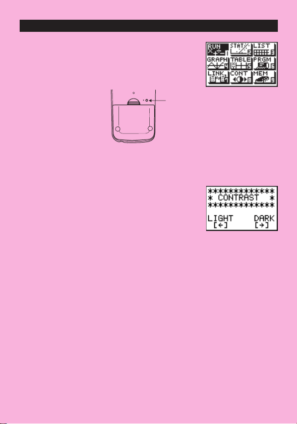
5. Press m.
If the Main Menu shown to the right is not on the display,
press the P button on the back of the calculator to
perform memory reset.
6. Use the cursor keys (
f, c, d, e) to select the CONT icon and press w
or simply press
i
to display the contrast adjustment screen.
7. Press d to make the figure on the screen lighter or e to make them darker.
8. After getting the contrast the way you want it, press
m to return to the main menu.
ii
P button

•Your calculator is made up of precision components. Never try to take it apart.
•Avoid dropping your calculator and subjecting it to strong impact.
•Do not store the calculator or leave it in areas exposed to high temperatures or humidity, or large
amounts of dust. When exposed to low temperatures, the calculator may require more time to display
results and may even fail to operate. Correct operation will resume once the calculator is brought back
to normal temperature.
• The display will go blank and keys will not operate during calculations. When you are operating the
keyboard, be sure to watch the display to make sure that all your key operations are being performed
correctly.
•Replace both the main power supply and the memory back up batteries once every 2 years regardless
of how much the calculator is used during that period. Never leave dead batteries in the battery com-
partment. They can leak and damage the unit.
•Keep batteries out of the reach of small children. If swallowed, consult with a physician immediately.
•Avoid using volatile liquids such as thinner or benzine to clean the unit. Wipe it with a soft, dry cloth, or
with a cloth that has been dipped in a solution of water and a neutral detergent and wrung out.
•In no event will the manufacturer and its suppliers be liable to you or any other person for any damages,
expenses, lost profits, lost savings or any other damages arising out of loss of data and/or formulas
arising out of malfunction, repairs, or battery replacement. The user should prepare physical records of
data to protect against such data loss.
•Never dispose of batteries, the liquid crystal panel, or other components by burning them.
•When the “Low battery!” message appears on the display, replace the main power supply batteries as
soon as possible.
•Be sure that the power switch is set to OFF when replacing batteries.
• If the calculator is exposed to a strong electrostatic charge, its memory contents may be damaged or
the keys may stop working. In such a case, perform the All Reset operation to clear the memory and
restore normal key operation.
•Note that strong vibration or impact during program execution can cause execution to stop or can
damage the calculator’s memory contents.
•Using the calculator near a television or radio can cause interference with TV or radio reception.
•Before assuming malfunction of the unit, be sure to carefully reread this manual and ensure that the
problem is not due to insufficient battery power, programming or operational errors.
Handling Precautions
iii

In no event shall CASIO Computer Co., Ltd. be liable to anyone for special, collateral, incidental, or
consequential damages in connection with or arising out of the purchase or use of these materials.
Moreover, CASIO Computer Co., Ltd. shall not be liable for any claim of any kind whatsoever against the
use of these materials by any other party.
• The contents of this manual are subject to change without notice.
•No part of this manual may be reproduced in any form without the express written consent of the
manufacturer.
• The options described in Chapter 9 of this manual may not be available in certain geographic areas.
For full details on availability in your area, contact your nearest CASIO dealer or distributor.
iv
Be sure to keep physical records of all important data!
The large memory capacity of the unit makes it possible to store large amounts of data. You should note,
however, that low battery power or incorrect replacement of the batteries that power the unit can cause
the data stored in memory to be corrupted or even lost entirely. Stored data can also be affected by
strong electrostatic charge or strong impact.

• ••••••••••••••••••
•••••••••••••••••••
• ••••••••••••••••••
•• •••••••••••••••••
• ••••••••••••••••••
•• •••••••••••••••••
•• •••••••••••••••••
•• •••••••••••••••••
•• • ••••••••••••••••
• ••••••••••••••••••
• ••••••••••••••••••
•• •••••••••••••••••
•• • ••••••••••••••••
• ••••••••••••••••••
• ••••••••••••••••••
•• •••••••••••••••••
•• • ••••••••••••••••
• ••••••••••••••••••
fx-7400G PLUS

Contents
vi
Chapter 1 Getting Acquainted ...................................................... 1
1. Using the Main Menu ............................................................................ 2
2. Key Table ............................................................................................... 4
3. Key Markings ........................................................................................ 6
4. Selecting Modes ................................................................................... 6
Using the Set Up Screen ............................................................................... 6
Set Up Screen Function Key Menus ............................................................. 7
5. Display ....................................................................................................9
About the Display Screen .............................................................................. 9
About Menu Item Types ................................................................................. 9
Exponential Display ..................................................................................... 10
Special Display Formats .............................................................................. 11
Calculation Execution Screen ...................................................................... 11
6. Contrast Adjustment .......................................................................... 11
7. When you keep having problems… .................................................. 12
Get the Calculator Back to its Original Mode Settings ................................ 12
Low Battery Message .................................................................................. 12
Chapter 2 Basic Calculations ..................................................... 13
1. Addition and Subtraction ................................................................... 14
2. Multiplication ...................................................................................... 14
3. Division .................................................................................................14
4. Quotient and Remainder Division ..................................................... 15
5. Mixed Calculations ............................................................................. 16
(1) Mixed Arithmetic Calculation Priority Sequence .................................... 16
(2) Parentheses Calculation Priority Sequence .......................................... 17
(3) Negative Values ..................................................................................... 17
(4) Exponential Expressions ....................................................................... 17
(5) Rounding ............................................................................................... 18
6. Other Useful Calculation Features .................................................... 18
(1) Answer Memory (Ans) ........................................................................... 18
(2) Consecutive Calculations ...................................................................... 18
(3) Replay .................................................................................................... 19
(4) Error Recovery ....................................................................................... 19
(5) Making Corrections ................................................................................ 20
7. Using Variables ................................................................................... 21

vii
Contents
8. Fraction Calculations ......................................................................... 23
(1) Fraction Display and Input ..................................................................... 23
(2) Performing Fraction Calculations ........................................................... 23
(3) Changing the Fraction Simplification Mode ........................................... 25
9. Selecting Value Display Modes.......................................................... 27
10. Scientific Function Calculations ....................................................... 28
(1) Trigonometric Functions ........................................................................ 28
Setting the Default Angle Unit ................................................................ 28
Converting Between Angle Units ........................................................... 29
Trigonometric Function Calculations ...................................................... 30
(2) Logarithmic and Exponential Function Calculations .............................. 30
(3) Other Functions ..................................................................................... 31
(4) Coordinate Conversion .......................................................................... 32
(5) Permutation and Combination ............................................................... 33
(6) Other Things to Remember ................................................................... 33
Multiplication Sign .................................................................................. 33
Calculation Priority Sequence ............................................................... 34
Using Multistatements ........................................................................... 34
Stacks .................................................................................................... 35
Errors ..................................................................................................... 36
How to Calculate Memory Usage .......................................................... 36
Memory Status (MEM) ........................................................................... 37
Clearing Memory Contents .................................................................... 37
Variable Data (VARS) Menu .................................................................. 38
Chapter 3 Differential Calculations ............................................43
Chapter 4 Graphing ..................................................................... 47
1. Before Trying to Draw a Graph .......................................................... 48
Entering the Graph Mode ............................................................................ 48
2. View Window (V-Window) Settings.................................................... 48
Initializing and Standardizing the View Window .......................................... 50
View Window Memory ................................................................................. 51
3. Graph Function Operations ............................................................... 52
Specifying the Graph Type .......................................................................... 52
Storing Graph Functions ............................................................................. 52
Editing Functions in Memory ....................................................................... 54
Drawing a Graph ......................................................................................... 54
4. Drawing Graphs Manually .................................................................. 55

viii
Contents
5. Other Graphing Functions ................................................................. 58
Connect Type and Plot Type Graphs (D-Type)............................................. 58
Trace ............................................................................................................ 59
Scroll ........................................................................................................... 60
Overwrite ..................................................................................................... 60
Zoom ........................................................................................................... 62
Sketch Function ........................................................................................... 65
Chapter 5 Table & Graph ............................................................. 73
1. Storing a Function .............................................................................. 74
2. Deleting a Function ............................................................................ 74
3. Assigning Values to a Variable........................................................... 74
4. Generating a Numeric Table ............................................................... 76
5. Editing a Table ..................................................................................... 77
6. Graphing a Function ........................................................................... 77
7. Assigning Numeric Table Contents to a List .................................... 78
Chapter 6 List Function .............................................................. 79
List Data Linking ..................................................................................... 80
1. List Operations ................................................................................... 81
2. Editing and Rearranging Lists ........................................................... 82
Editing List Values ....................................................................................... 82
Sorting List Values ....................................................................................... 85
3. Manipulating List Data ....................................................................... 87
Accessing the List Data Manipulation Function Menu ................................. 87
4. Arithmetic Calculations Using Lists ................................................. 91
Error Messages ........................................................................................... 91
Inputting a List into a Calculation ................................................................ 91
Recalling List Contents ................................................................................ 93
Graphing a Function Using a List ................................................................ 93
Inputting Scientific Calculations into a List .................................................. 93
Performing Scientific Function Calculations Using a List ............................ 94
Chapter 7 Statistical Graphs and Calculations .........................95
1. Before Performing Statistical Calculations ...................................... 96
2. Statistical Calculation Examples ....................................................... 96
Inputting Data into Lists ............................................................................... 97

ix
Contents
Plotting Data ................................................................................................ 97
Plotting a Scatter Diagram........................................................................... 98
Changing Graph Parameters....................................................................... 98
1. Graph draw/non-draw status (SELECT) .................................................. 98
2. General graph settings (SET) .................................................................. 99
Drawing an
xy Line Graph ......................................................................... 105
Selecting the Regression Type .................................................................. 105
Displaying Statistical Calculation Results .................................................. 106
Graphing statistical calculation results ...................................................... 106
3. Calculating and Graphing Single-Variable Statistical Data ........... 107
Histogram .................................................................................................. 107
Box Graph ................................................................................................. 107
Normal Distribution Curve ......................................................................... 108
Displaying Single-Variable Statistical Results ........................................... 108
Pie Chart ................................................................................................... 109
Stacked Bar Chart ..................................................................................... 110
Bar Graph .................................................................................................. 111
Line Graph ................................................................................................. 112
Bar Graph and Line Graph ........................................................................ 113
4. Calculating and Graphing Paired-Variable Statistical Data ........... 114
Linear Regression Graph .......................................................................... 114
Med-Med Graph ........................................................................................ 115
Quadratic Regression Graph ..................................................................... 115
Logarithmic Regression Graph .................................................................. 116
Exponential Regression Graph.................................................................. 116
Power Regression Graph .......................................................................... 117
Displaying Paired-Variable Statistical Results ........................................... 118
Copying a Regression Graph Formula to the Graph Mode ....................... 118
Multiple Graphs ......................................................................................... 119
5. Manual Graphing .............................................................................. 120
Setting the Width of a Histogram ............................................................... 120
6. Performing Statistical Calculations................................................. 121
Single-Variable Statistical Calculations ..................................................... 122
Paired-Variable Statistical Calculations ..................................................... 122
Regression Calculation ............................................................................. 123
Estimated Value Calculation (
, ) ............................................................ 123

x
Contents
Chapter 8 Programming ........................................................... 125
1. Before Programming ........................................................................ 126
2. Programming Examples................................................................... 127
3. Debugging a Program ...................................................................... 132
4. Calculating the Number of Bytes Used by a Program ................... 132
5. Secret Function ................................................................................ 133
6. Searching for a File........................................................................... 134
7. Editing Program Contents ............................................................... 135
8. Deleting a Program ........................................................................... 138
9. Useful Program Commands............................................................. 139
10. Command Reference ........................................................................ 143
Command Index ........................................................................................ 143
Basic Operation Commands ..................................................................... 144
Program Commands (COM) ...................................................................... 145
Program Control Commands (CTL) ........................................................... 149
Jump Commands (JUMP) ......................................................................... 151
Clear Commands (CLR) ............................................................................ 153
Display Commands (DISP) ........................................................................ 153
Input / Output Commands (I/O) ................................................................. 154
Conditional Jump Relational Operators (REL) .......................................... 155
11. Text Display ....................................................................................... 156
12. Using Calculator Functions in Programs ....................................... 156
Using Graph Functions in a Program ........................................................ 156
Using Table & Graph Functions in a Program ........................................... 157
Using List Sort Functions in a Program ..................................................... 158
Using Statistical Calculations and Graphs in a Program ........................... 158
Performing Statistical Calculations ............................................................ 160
Chapter 9 Data Communications ............................................. 163
1. Connecting Two Units ...................................................................... 164
2. Connecting the Unit with a Personal Computer ............................. 165
3. Connecting the Unit with a CASIO Label Printer ........................... 166
4. Before Performing a Data Communication Operation ................... 167
5. Performing a Data Transfer Operation ............................................ 168
6. Screen Send Function ...................................................................... 172
7. Data Communications Precautions ................................................ 173

xi
Contents
Chapter 10 Program Library ..................................................... 175
1. Prime Factor Analysis ...................................................................... 176
2. Greatest Common Measure ............................................................. 178
3.
t-Test Value ....................................................................................... 180
4. Circle and Tangents .......................................................................... 182
5. Rotating a Figure .............................................................................. 189
Appendix ..................................................................................... 193
Appendix A Resetting the Calculator ................................................... 194
Appendix B Power Supply .................................................................... 196
Replacing Batteries ................................................................................... 196
About the Auto Power Off Function ........................................................... 199
Appendix C Error Message Table ......................................................... 200
Appendix D Input Ranges ..................................................................... 202
Appendix E Specifications .................................................................... 204

xii
Contents

Getting Acquainted
— Read This First!
1
Chapter
: Important notes
: Notes
: Reference pages
The symbols in this manual indicate the
following messages.
P. 000
2
Chapter 1 Getting Acquainted
1. Using the Main Menu
The main menu appears on the display whenever you turn on the calculator. It con-
tains a number of icons that let you select the mode (work area) for the type of
operation you want to perform. You can also make the Main Menu appear at any time
by pressing m.
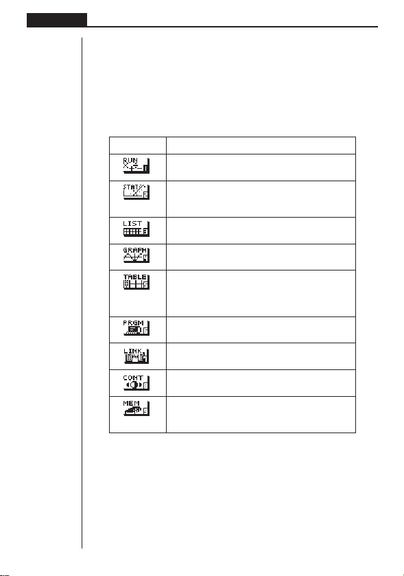
The following explains the meaning of each icon.
Icon Meaning
Use this mode for arithmetic calculations and func-
tion calculations.
Use this mode to perform single-variable (stand-
ard deviation) and paired-variable (regression) sta-
tistical calculations, and to draw statistical graphs.
Use this mode for storing and editing numeric
data.
Use this mode to store graph functions and to
draw graphs using the functions.
Use this mode to store functions, to generate a
numeric table of different solutions as the values
assigned to variables in a function change, and
to draw graphs.
Use this mode to store programs in the program
area and to run programs.
Use this mode to transfer memory contents or
back-up data to another unit.
Use this mode to adjust the contrast of the dis-
play.
Use this mode to check how much memory is
used and remaining, to delete data from memory,
and to initialize (reset) the calculator.
3
Getting Acquainted Chapter 1
uu
uu
uTo enter a mode
Example To enter the RUN Mode from the Main Menu
1. Press m to display the Main Menu.
2. Use d, e, f, and c to move the highlighting to the RUN icon.
3. Press w to enter the RUN Mode.
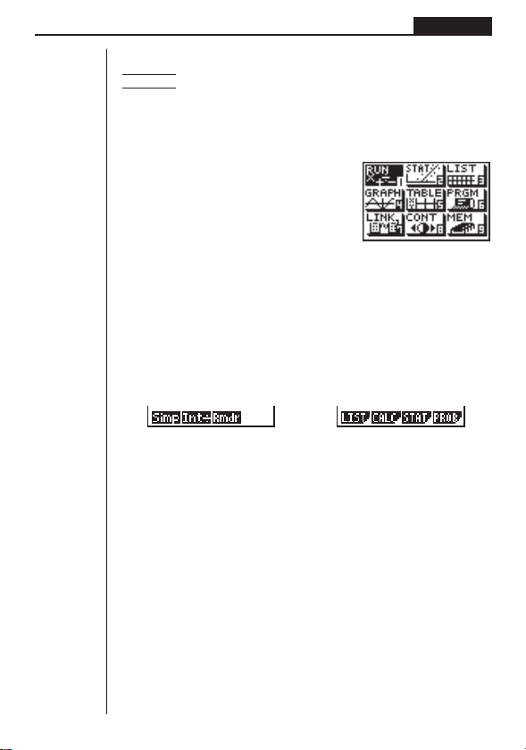
•You can also enter a mode without highlighting an icon in the Main Menu by
inputting the number marked in the lower right corner of the icon.
•When you enter a mode, up to four function key menu items appear at the bottom
of the display. Each menu item corresponds to the function key (1, 2, 3,
4) that is below the item. Some function menus have multiple pages. When this
happens, you should press [ to advance to the next menu page.
Example Menus
1234 1234
4
Chapter 1 Getting Acquainted
Alpha Lock
Normally, once you press a and then a key to input an alphabetic char-
acter, the keyboard reverts to its primary functions immediately. If you press
! and then a, the keyboard locks in alpha input until you press a
again.
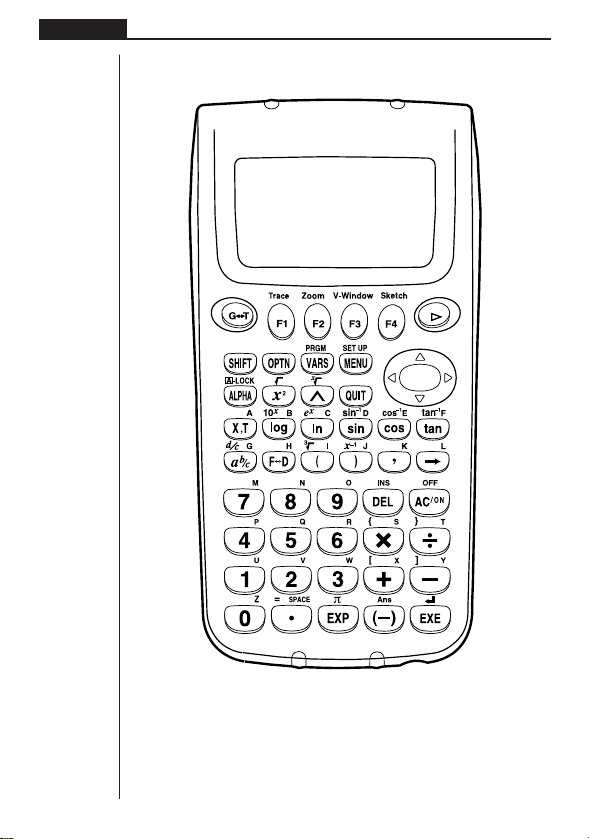
2. Key Table

5
Getting Acquainted Chapter 1
Page
PagePagePagePage
Page
Page PagePagePagePage
6
6
45
23
24 31
15
31
31
31
31
23
38
139
31
31
31
31
17
31
2
7
16
30
17
30
82
30
21
60
17
30
17
18
14
60
14
82
20
21
16
60
14
82
Trace Zoom
Sketch
V-Window
6
Chapter 1 Getting Acquainted
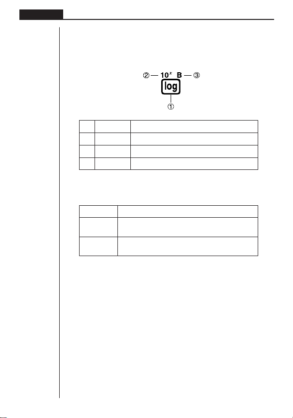
3. Key Markings
Many of the calculator’s keys are used to perform more than one function. The func-
tions marked on the keyboard are color coded to help you find the one you need
quickly and easily.
Function Key Operation
1 log l
2 10
x
!l
3 B al
The following describes the color coding used for key markings.
Color Key Operation
Orange Press ! and then the key to perform the marked
function.
RedPress a and then the key to perform the marked
function.
4. Selecting Modes
kk
kk
k Using the Set Up Screen
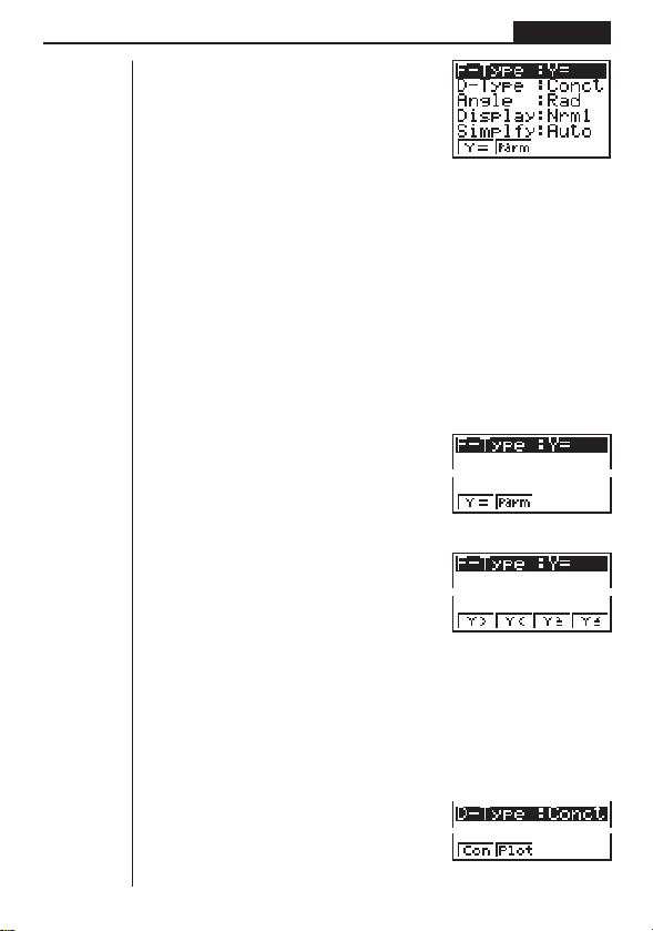
The first thing that appears when you enter a mode is the mode’s set up screen,
which shows the current status of settings for the mode. The following procedure
shows how to change a set up.
uu
uu
uTo change a mode set up
1. Select the icon you want and press w enter a mode and display its initial screen.
Here we will enter the RUN Mode.
7
Getting Acquainted Chapter 1
2. Press !Z to display the mode’s set up
screen.
• This set up screen is just one possible exam-
ple. Actual set up screen contents will differ
according to the mode you are in and that
mode’s current settings.
3. Use the f and c cursor keys to move the highlighting to the item whose
setting you want to change.
4. Press the function key (1 to 4) that is marked with the setting you want to
make.
5. After you are finished making any changes you want, press Q to return to the
initial screen of the mode.
kk
kk
k Set Up Screen Function Key Menus
This section details the settings you can make using the function keys in the set up
display.
uu
uu
uGraph Function Type (F-Type)
1 (Y=) .......... Rectangular coordinate
graphs
2 (Parm) ...... Parametric coordinate graphs
[
1 (Y>) .......... y > f(x) inequality graph
2 (Y<) .......... y < f(x) inequality graph
3 (Y≥) .......... y > f (x) inequality graph
4 (Y≤) .......... y < f (x) inequality graph
Press [ to return to the previous menu.
• The setting you make for F-Type determines the variable name that is input when
you press T.
uu
uu
uGraph Draw Type (D-Type)
1 (Con) ........ Connection of points plot-
ted on graph.
2 (Plot) ......... Plotting of points on graph
without connection.
1234
1234[
1234[
1234
8
Chapter 1 Getting Acquainted
uu
uu
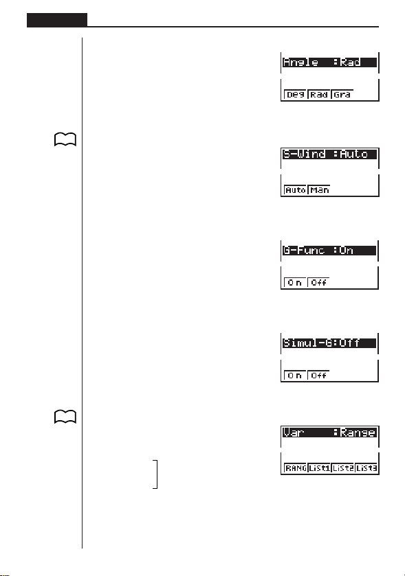
uAngle unit (Angle)
1 (Deg) ........ Specifies degrees as
default.
2 (Rad) ........ Specifies radians as
default.
3 (Gra) ......... Specifies grads as default.
uu
uu
uStatistical Graph View Window Setting (S-Wind)
1 (Auto) ........ Automatic setting of view
window values for statisti-
cal graph drawing.
2 (Man) ........ Manual setting of view
window values for statisti-
cal graph drawing.
uu
uu
uGraph Function Display (G-Func)
1 (On) .......... Turns on display of function
during graph drawing and
trace.
2 (Off) .......... Turns off display of function
during graph drawing and
trace.
uu
uu
uSimultaneous Graph Mode (Simul-G)
1 (On) .......... Turns on simultaneous
graphing of all functions in
memory.
2 (Off) .......... Simultaneous graphing off
(graphs drawn one-by-
one).
uu
uu
uTable & Graph Generation Settings (Var)
1 (RANG) .... Table generation and graph
drawing using numeric ta-
ble range.
2 (List1)
3 (List2)
....
4 (List3)
P. 120
P. 120
1234
1234
1234
1234
Table generation and graph
drawing using list data.
P. 7 5
1234[

9
Getting Acquainted Chapter 1
[
1 (List4)
2 (List5)
....
3 (List6)
Press [ to return to the previous menu.
Other menus for set up (Display, Simplfy, Frac) are described in each applicable
section of this manual as they come up.
Abbreviations
STAT ............... Statistics
PRGM ............. Program
CONT.............. Contrast
MEM ............... Memory
5. Display
kk
kk
k About the Display Screen
This calculator uses two types of display: a text display and a graphic display. The
text display can show 13 columns and six lines of characters, with the bottom line
used for the function key menu, while the graph display uses an area that measures
79 (W) × 47 (H) dots.
Text Display Graph Display
kk
kk
k About Menu Item Types
This calculator uses certain conventions to indicate the type of result you can expect
when you press a function key.
• Next Menu
Example:
Selecting displays a menu of list functions.
• Command Input
Example:
Selecting inputs the “List” command.
Table generation and graph
drawing using list data.
1234 [
10
Chapter 1 Getting Acquainted
• Direct Command Execution
Example:
Selecting executes the DRAW command.
kk
kk
k Exponential Display
The calculator normally displays values up to 10 digits long. Values that exceed this
limit are automatically converted to and displayed in exponential format. You can
specify one of two different ranges for automatic changeover to exponential display.
Norm 1 ............ 10
–2
(0.01) > |x|, |x| > 10
10
Norm 2 ............ 10
–9
(0.000000001) > |x|, |x| > 10
10
uu
uu
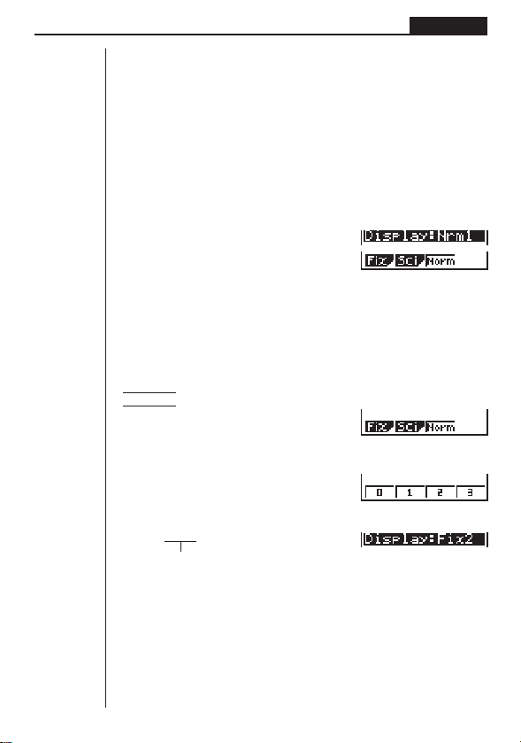
uTo change the exponential display range
1. Press !Z to display the Set Up Screen.
2. Use f and c to move the highlighting to “Display”.
3. Press 3 (Norm).
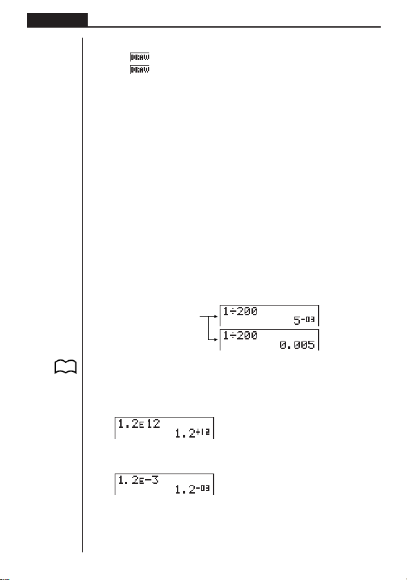
The exponential display range switches between Norm 1 and Norm 2 each time you
perform the above operation. There is no display indicator to show you which expo-
nential display range is currently in effect, but you can always check it by seeing what
results the following calculation produces.
Ab/caaw
(Norm 1)
(Norm 2)
All of the examples in this manual show calculation results using Norm 1.
For full details about the “Display”, see “Selecting Value Display Modes”.
uu
uu
uHow to interpret exponential format
1.2
+12
indicates that the result is equivalent to 1.2 × 10
12
. This means that you should
move the decimal point in 1.2 twelve places to the right, because the exponent is
positive. This results in the value 1,200,000,000,000.
1.2
–03
indicates that the result is equivalent to 1.2 × 10
–3
. This means that you should
move the decimal point in 1.2 three places to the left, because the exponent is nega-
tive. This results in the value 0.0012.
P. 2 7
11
Getting Acquainted Chapter 1
kk
kk
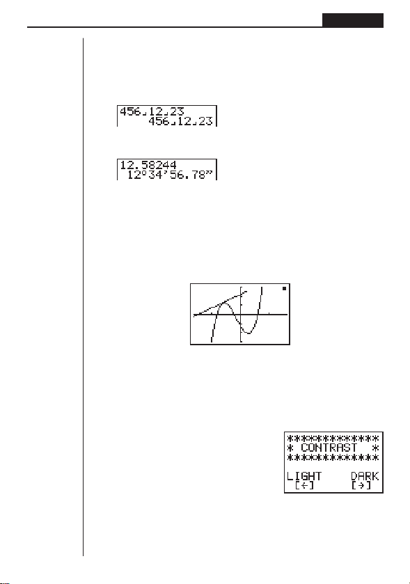
k Special Display Formats
This calculator uses special display formats to indicate fractions, and sexagesimal
values.
uu
uu
uFractions
.......... Indicates: 456
uu
uu
uSexagesimal Values
.......... Indicates: 12° 34’ 56.78"
•In addition to the above, this calculator also uses other indicators or symbols,
which are described in each applicable section of this manual as they come up.
kk
kk
k Calculation Execution Screen
Whenever the calculator is busy drawing a graph or executing a long, complex calcu-
lation or program, a black box (k) flashes in the upper right corner of the display.
This black box tells you that the calculator is performing an internal operation.
6. Contrast Adjustment
Adjust the contrast whenever objects on the display appear dim or difficult to see.
uu
uu
uTo display the contrast adjustment screen
Highlight the CONT icon in the Main Menu and
then press w.
Press d to make the figures on the screen lighter or e to make them darker.
After getting the contrast the way you want it, press m to return to the main menu.
12
–––
23

12
Chapter 1 Getting Acquainted
7. When you keep having problems…
If you keep having problems when you are trying to perform operations, try the fol-
lowing before assuming that there is something wrong with the calculator.
kk
kk
k Get the Calculator Back to its Original Mode Settings
1. In the Main Menu, select the RUN icon and press w.
2. Press ! Z to display the Set Up Screen.
3. Highlight “Angle” and press 2 (Rad).
4. Highlight “Display” and press 3 (Norm) to select the exponential display range
(Norm 1 or Norm 2) that you want to use.
5. Now enter the correct mode and perform your calculation again, monitoring the
results on the display.
kk
kk
k Low Battery Message
The low battery message appears while the main battery power is below a certain
level whenever you press o to turn power on or m to display the Main Menu.
o or m
↓
About 3 seconds later
If you continue using the calculator without replacing batteries, power will automati-
cally turn off to protect memory contents. Once this happens, you will not be able to
turn power back on, and there is the danger that memory contents will be corrupted
or lost entirely.
P. 6
P. 196

Basic Calculations
In the RUN Mode you can perform arithmetic calculations (addi-
tion, subtraction, multiplication, division) as well as calculations in-
volving scientific functions.
1. Addition and Subtraction
2. Multiplication
3. Division
4. Quotient and Remainder Division
5. Mixed Calculations
6. Other Useful Calculation Features
7. Using Variables
8. Fraction Calculations
9. Selecting Value Display Modes
10. Scientific Function Calculations
Chapter
2
14
Chapter 2 Basic Calculations
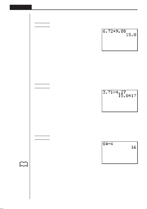
1. Addition and Subtraction
Example 6.72 + 9.08
g.hc+j.aiw
You can input the operation just as it is written. This capability is called “true alge-
braic logic.”
Be sure to press A to clear the display before starting a new calculation.
2. Multiplication
Example 3.71 × 4.27
Ad.hb*
e.chw
• The range of this calculator is –9.99999999 × 10
99
to +9.99999999 × 10
99
.
3. Division
Example 64 ÷ 4
Age/ew
Parentheses also come in handy when performing division. For full details on using
parentheses, see “Parentheses Calculation Priority Sequence”.
P. 1 7
15
Basic Calculations Chapter 2
uu
uu
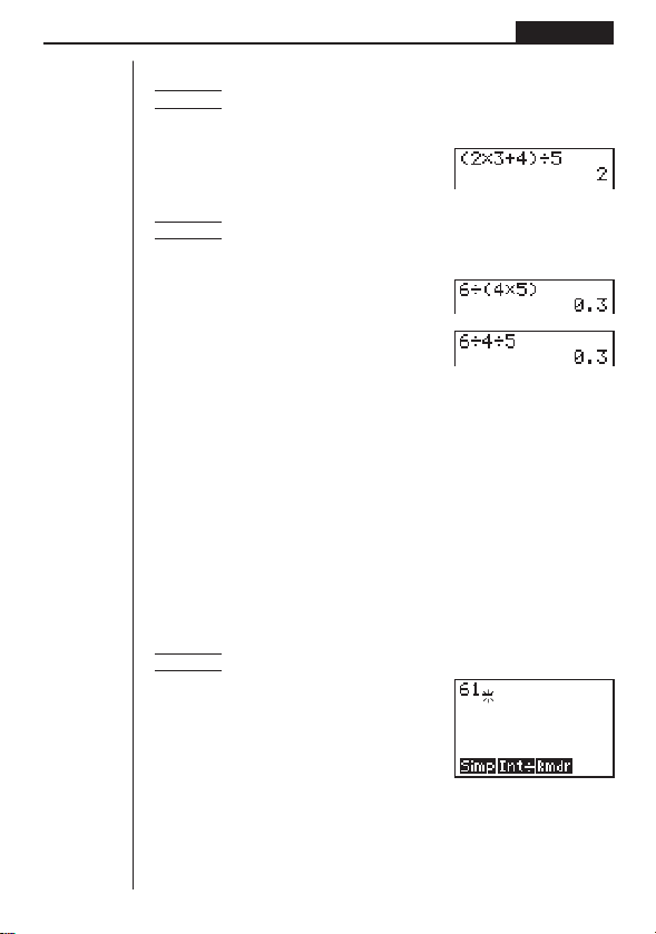
uTo use parentheses in a calculation
2 × 3 + 4
Example 1
–––––––
5
You should input this calculation as: (2 × 3 + 4) ÷ 5
A(c*d+e)/fw
6
Example 2 –––––
4 × 5
You can input this calculation as: 6 ÷ (4 × 5) or 6 ÷ 4 ÷ 5.
Ag/(e*f)w
Ag/e/fw
4. Quotient and Remainder Division
This calculator can produce either the quotient or the quotient and remainder of
division operations involving two integers. Use K to display the Option Menu for
the function key menu you need to perform quotient and remainder division.
Operation
Use the RUN Mode for quotient and remainder division.
Quotient Division ...... <integer>K2(CALC)2(Int÷)<integer>w
Reminder Division .... <integer>K2(CALC)3(Rmdr)<integer>w
uu
uu
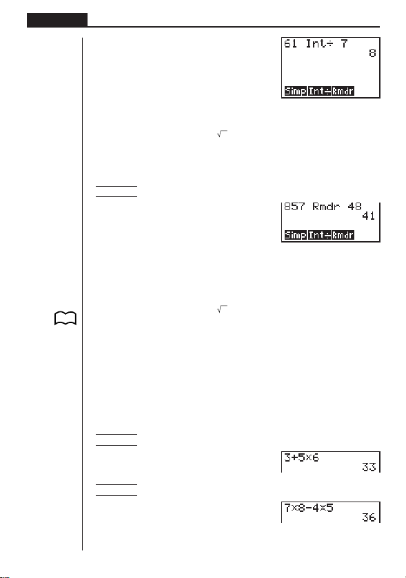
uTo perform quotient division
Example To display the quotient produced by 61 ÷ 7
AgbK2(CALC)
1 2 34
16
Chapter 2 Basic Calculations
2(Int÷)hw
•Remember that you can use only integers in quotient division operations. You
cannot use expressions such as
2 or sin60 because their results have a decimal
part.
uu
uu
uTo perform remainder division
Example To display the remainder produced by 857 ÷ 48
ifh3(Rmdr)eiw
Press Q to clear the Option Menu after you finish your remainder and quotient
calculations.
•Remember that you can use only integers in remainder division operations. You
cannot use expressions such as
2 or sin60 because their results have a decimal
part.
•Quotient and remainder division can also be used with lists to divide a multiple
integers by each other in a single operation.
5. Mixed Calculations
(1) Mixed Arithmetic Calculation Priority Sequence
For mixed arithmetic calculations, the calculator automatically performs multiplica-
tion and division before addition and subtraction.
Example 1 3 + 5 × 6
Ad+f*gw
Example 2 7 × 8 – 4 × 5
Ah*i-e*fw
1 2 34
123 4
P. 9 1

17
Basic Calculations Chapter 2
(2) Parentheses Calculation Priority Sequence
Expressions enclosed inside parentheses are always given priority in a calculation.
Example 1 100 – (2 + 3) × 4
Abaa-(c+d)
*ew
Example 2 (7 – 2) × (8 + 5)
•A multiplication sign immediately in front of an open parenthesis can be omitted.
A(h-c)(i+f)
w
•Any closing parentheses at the end of a calculation can be omitted, no matter
how many there are.
Parentheses are always closed in the operation examples presented in this manual.
(3) Negative Values
Use the - key to input negative values.
Example 56 × (–12) ÷ (–2.5)
Afg*-bc/
-c.fw
(4) Exponential Expressions
Use the E key to input exponents.
Example (4.5 × 10
75
) × (–2.3 × 10
–79
)
Ae.fEhf*-c.d
E-hjw
The above shows what would appear when the exponential display range is set to
Norm 1. It stands for –1.035 × 10
–3
, which is –0.001035.
P. 1 0

18
Chapter 2 Basic Calculations
(5) Rounding
Example 74 ÷ 3
Ahe/dw
The actual result of the above calculation is 24.66666666… (and so on to infinity),
which the calculator rounds off. The calculator’s internal capacity is 15 digits for the
values it uses for calculations, which avoids precision problems with consecutive
operations that use the result of the previous operation.
6. Other Useful Calculation Features
(1) Answer Memory (Ans)
Calculation results are automatically stored in the Answer Memory, which means
you can recall the results of the last calculation you performed at any time.
uu
uu
uTo recall Answer Memory contents
Press ! and then K (which is the shifted function of the - key).
This operation is represented as ! K throughout this manual.
Example To perform 3.56 + 8.41 and then divide 65.38 by the result
Ad.fg+i.ebw
gf.di/!Kw
(2) Consecutive Calculations
If the result of the last calculation is the first term of the next calculation, you can use
the result as it is on the display without recalling Answer Memory contents.
uu
uu
uTo perform a consecutive calculation
Example To perform 0.57 × 0.27, and then add 4.9672 to the results
Aa.fh*a.chw
+e.jghcw
19
Basic Calculations Chapter 2
(3) Replay
While the result of a calculation is on the display, you can use d and e to move the
cursor to any position within the expression used to produce the result. This means
you can back up and correct mistakes without having to input the entire calculation.
You can also recall past calculations you have already cleared by pressing A.
Operation
The first press of e displays the cursor at the beginning of the expression, while
d displays the cursor at the end. Once the cursor is displayed, use e to move it
right and d to move it left.
uu
uu
uTo use Replay to change an expression
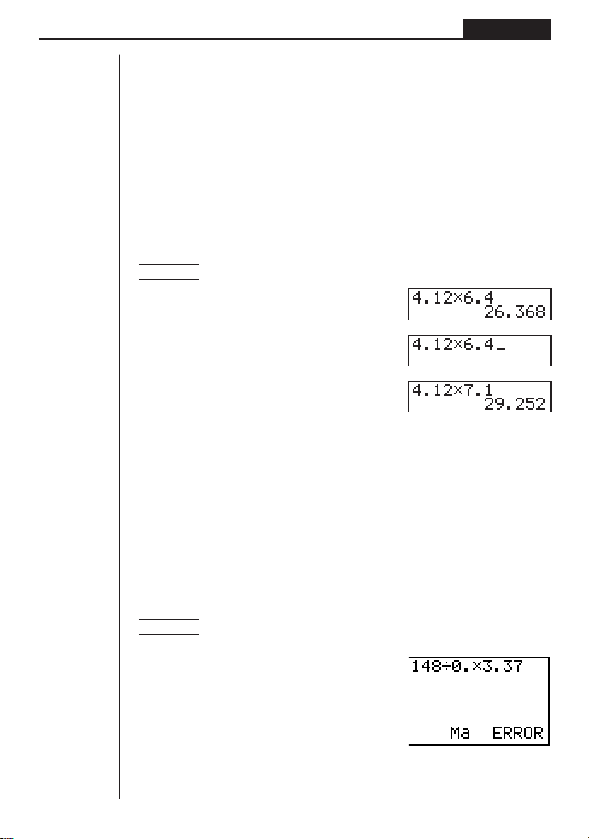
Example To calculate 4.12 × 6.4 and then change the calculation to 4.12 × 7.1
Ae.bc*g.ew
d
dddh.bw
Multi-Replay
Pressing A and then f or c sequentially recalls and displays past calculations.
(4) Error Recovery
Whenever an error message appears on the display, press d or e to re-display
the expression with the cursor located just past the part of the expression that caused
the error. You can then move the cursor and make necessary corrections before
executing the calculation again.
uu
uu
uTo correct an expression that causes an error
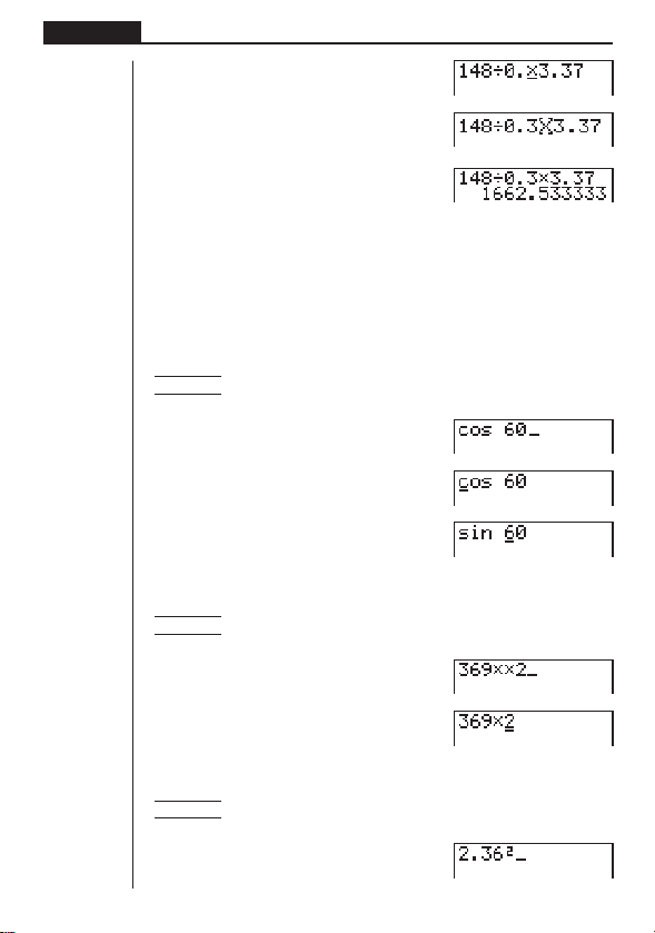
Example To recover from the error generated by performing 148 ÷ 0. × 3.37
instead of 148 ÷ 0.3 × 3.37
Abei/a.
*d.dhw
20
Chapter 2 Basic Calculations
d(You could also press e.)

21
Basic Calculations Chapter 2
ddddd

22
Chapter 2 Basic Calculations
uu
uu
uTo assign the same value to more than one variable
Operation
<value or expression>aa<start variable name>a3(~)a<end variable
name>w
Example To assign the result of 2 to variables A, B, C, D, and E
A!9caaAa3(~)
aEw
uu
uu
uTo clear the contents of all variables
In the Main Menu, select the MEM icon and press w.
Select Memory Usage.
w
Press c to scroll the display until “Alpha” is highlighted.
ccccccc
1(DEL)
Press 1 (YES) to clear all variables or 4 (NO) to abort the clear operation without
clearing anything.
1 234
1 234

23
Basic Calculations Chapter 2
8. Fraction Calculations
(1) Fraction Display and Input
Example 1 Display of
Example 2 Display of 3
Mixed fractions (such as 3 1/4) are input and displayed as:
integer{numerator{denominator.
Improper fractions (15/7) and proper fractions (such as 1/4) are input and displayed
as: numerator{denominator.
Use the $ key to input each part of a fraction.
uu
uu
uTo input a fraction
Operation
Proper Fraction or Improper Fraction Input: <numerator value>$<denominator value>
Mixed Fraction Input: <integer value>$<numerator value>$<denominator value>
Example To input 3
Press d$b$e.
Note that the maximum size of a fractional value is 10 digits, counting the integer,
numerator, and denominator digits and separator symbols. Any value longer than
10 digits is automatically converted to its equivalent decimal value.
(2) Performing Fraction Calculations
Example
Ac$f+d$b$ew
uu
uu
uTo convert between fraction and decimal values
Operation
Fraction to Decimal Conversion: M
Decimal to Fraction Conversion: M
21
–– + 3––
54
3
––
4
1
––
4
1
––
4

24
Chapter 2 Basic Calculations
Example To convert the result of the previous example to a decimal and
then back to a fraction
M
M
uu
uu
uTo convert between proper and improper fractions
Operation
Mixed Fraction to Improper Fraction Conversion: !/
Improper Fraction to Mixed Fraction Conversion: !/
Example To convert the result of the previous example to an improper
fraction and then back to a proper fraction
!/
!/
• The calculator automatically reduces the results of fraction calculations. You can
use the procedure described under “Changing the Fraction Simplification Mode”
below to specify manual fraction simplification.
uu
uu
uTo perform a mixed decimal and fraction calculation
Example 5.2 ×
Af.c*b$fw
• The result of a calculation that mixes fractions and decimal values is always a
decimal value.
uu
uu
uTo use parentheses in a fraction calculation
Example
Ab$(b$d+b$e)
+c$hw
1
––
5
12
–––––– + ––
117
–– + ––
34
25
Basic Calculations Chapter 2
(3) Changing the Fraction Simplification Mode
The initial default of the calculator is automatic simplification of fractions produced
by fraction calculations. You can use the following operation to change the fraction
simplification mode to manual.
uu
uu
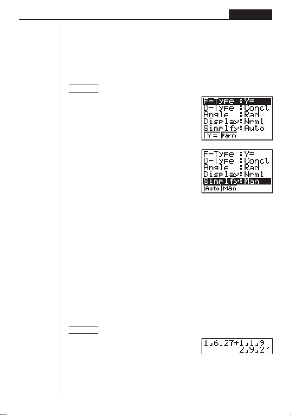
uTo change the fraction simplification mode
Example To change the fraction simplification mode to manual
!Z
(Displays the Set Up Screen.)
cccc2(Man)
When the fraction simplification is set to manual, you have to use the Option Menu to
simplify fractions. You can let the calculator select the divisor to use for simplification
or you can specify a divisor.
uu
uu
uTo simplify using the calculator’s divisor
Operation
Perform calculations after selecting the RUN icon in the Main Menu to enter the
RUN Mode.
To display the simplification menu: K2(CALC)
To select automatic simplification: 1(Simp)w
To specify the divisor for simplification*: 1(Simp) <Divisor>w
*You can specify only a positive integer as the divisor.
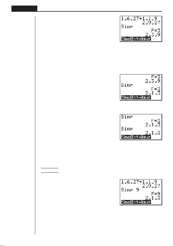
61
Example To perform the calculation 1
––
+ 1
–– and reduce the result
27 9
Ab$g$ch+b$
b$jw
(The result that appears when using manual simplification is the least common mul-
tiple of the fractions used in the calculation.)
1 2 34
26
Chapter 2 Basic Calculations
K2(CALC)1(Simp)w
•F = 3 indicates that 3 is the divisor.
• The calculator automatically selects the smallest possible divisor for simplifica-
tion.
Repeat the above operation to simplify again.
1(Simp)w
Try once again.
1(Simp)w
This display indicates that further simplification is impossible.
uu
uu
uTo simplify using your own divisor
ExampleTo perform the above calculation and then specify 9 as the divisor
to use for simplification
1(Simp)jw
• If the value you specify is invalid as a divisor for simplification, the calculator
automatically uses the lowest possible divisor.
1 234
1 234
1 234
1 234
27
Basic Calculations Chapter 2
9. Selecting Value Display Modes
You can make specifications for three value display modes.
Fix Mode
This mode lets you specify the number of decimal places to be displayed.
Sci Mode
This mode lets you specify the number of significant digits to be displayed.
Norm 1/Norm 2 Mode
This mode determines at what point the display changes over to exponential display
format.
Display the Set Up Screen and use the f and c keys to highlight “Display”.
uu
uu
u To specify the number of decimal places (Fix)
1. While the set-up screen is on the display, press 1 (Fix).
2. Press the function key that corresponds to the number of decimal places you
want to set (0 to 9).
•Press [ to display the next menu of numbers.
Example To specify two decimal places
1 (Fix)
3 (2)
Press the function key that corresponds to the
number of decimal places you want to specify.
•Displayed values are rounded off to the number of decimal places you specify.
•A number of decimal place specification remains in effect until you change the
Norm Mode setting.
1234
1 234
123 4
28
Chapter 2 Basic Calculations
uu
uu
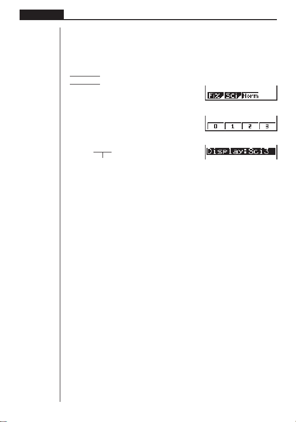
u To specify the number of significant digits (Sci)
1. While the set-up screen is on the display, press 2 (Sci).
2. Press the function key that corresponds to the number of significant digits you
want to set (0 to 9).
•Press [ to display the next menu of numbers.
Example To specify three significant digits
2 (Sci)
4 (3)
Press the function key that corresponds to the
number of significant digits you want to specify.
•Displayed values are rounded off to the number of significant digits you specify.
•Specifying 0 makes the number of significant digits 10.
•A number of significant digit specification remains in effect until you change the
Norm Mode setting.
uu
uu
u To specify the exponential display range (Norm 1/Norm 2)
Press 3 (Norm) to switch between Norm 1 and Norm 2.
Norm 1: 10
–2
(0.01)>|x|, |x| >10
10
Norm 2: 10
–9
(0.000000001)>|x|, |x| >10
10
10. Scientific Function Calculations
Use the RUN Mode to perform calculations that involve trigonometric functions and
other types of scientific functions.
(1) Trigonometric Functions
Before performing a calculations that involves trigonometric functions, you should
first specify the default angle unit as degrees (°), radians (r), or grads (g).
kk
kk
k Setting the Default Angle Unit
The default angle unit for input values can be set using the set up screen. If you set
degrees (°) for example, inputting a value of 90 is automatically assumed to be 90°
The following shows the relationship between degrees, radians, and grads.
90° = π/2 radians = 100 grads
1 2 34
1234
29
Basic Calculations Chapter 2
uu
uu
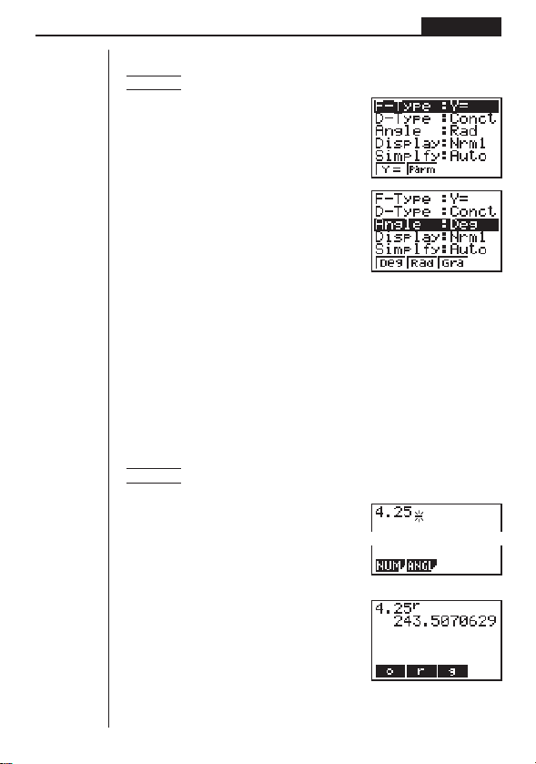
uTo set the default angle unit
Example To change the angle unit from radians to degrees
!Z
cc1(Deg)
•Once you change the angle unit setting, it remains in effect until you change it
again using the set up screen. You also should check the set up screen to find out
what the current angle unit setting is.
kk
kk
k Converting Between Angle Units
You can use the following procedure to input a value using an angle unit that is not
the current default angle unit. Then when you press w, the value will be converted
to the default angle unit.
uu
uu
uTo convert between angle units
Example To convert 4.25 radians to degrees while degrees are set as the
default angle unit
Ae.cfK[
2(ANGL)2(r)w
1 2 34
1 2 34
1 234

30
Chapter 2 Basic Calculations
kk
kk
k Trigonometric Function Calculations
Always make sure that the default angle unit is set to the required default before
performing trigonometric function calculations.
uu
uu
uTo perform trigonometric function calculations
Example 1 sin (63° 52' 41")
Default angle unit: Degrees
!Zcc1(Deg)Q
sgdK[2(ANGL)[1(° ' ")fc1(° ' ")eb1(° ' ")w
Result: 0.897859012
Example 2
Default angle unit: Radians
!Zcc2(Rad)Q
b/c(!7/d)w
Result: 2
Example 3 tan(–35grad)
Default angle unit: Grads
!Zcc3(Gra)Q
t-dfw
Result: –0.6128007881
(2) Logarithmic and Exponential Function Calculations
•A base 10 logarithm (common logarithm) is normally written as log10 or log.
•A base e () logarithm (natural logarithm) is normally
written as log
e or ln.
Note that certain publications use “log” to refer to base
e logarithms, so you must
take care to watch for what type of notation is being used in the publications you are
working with. This calculator and manual use “log” to mean base 10 and “ln” for base
e.
P. 2 9
π
1
sec (–– rad) = ––––––––––
3
π
cos (––rad)
3
1
n
lim
1 + ––– = 2.71828...
n
n→∞

31
Basic Calculations Chapter 2
uu
uu
uTo perform logarithmic/exponential function calculations
Example 1 log1.23
lb.cdw
Result: 0.0899051114
Example 2 ln90
Ijaw
Result: 4.49980967
Example 3 To calculate the anti-logarithm of common logarithm 1.23 (10
1.23
)
!0b.cdw
Result: 16.98243652
Example 4 To calculate the anti-logarithm of natural logarithm 4.5 (e
4.5
)
!ee.fw
Result: 90.0171313
Example 5 (–3)
4
= (–3) × (–3) × (–3) × (–3)
(-d)Mew
Result: 81
Example 6
7
123
h!qbcdw
Result: 1.988647795
(3) Other Functions
Example Operation Display
+
=
3.65028154 !92+!95w 3.6502815425
(–3)
2
= (–3) × (–3) = 9 (-3)xw 9
–3
2
= –(3 × 3) = –9 -3xw – 9
(3!X-4!X)
!Xw 12
8! (= 1 × 2 × 3 × .... × 8)
= 40320 8K4(PROB)1(
x!)w 40320
3
= 42
!#(36*42*49)w
4236 × 42 × 49
Random number generation K4(PROB)
(pseudo random number 4(Ran#)w (Ex.) 0.4810497011
between 0 and 1.)
1
––––––––––– = 12
11
––– – –––
34
32
Chapter 2 Basic Calculations
Example Operation Display
What is the absolute value of
the common logarithm of
3
?
4
|
log
3
|
= 0.1249387366
K[1(NUM)
4
1(Abs)l(3/4)w 0.1249387366
What is the integer part of K[1(NUM)
2(Int)(7800/96)w 81
What is the decimal part of K[1(NUM)
3(Frac)(7800/96)w 0.25
200 ÷ 6= 200/6w 33.33333333
× 3= *3w 100
Round the value used 200/6w 33.33333333
for internal calculations K[ 1(NUM)4(Rnd)w 33.33333333
to 11 digits* *3w 99.99999999
What is the nearest integer K[1(NUM)[1(Intg)
not exceeding – 3.5? -3.5w – 4
*When a Fix (number of decimal places) or Sci (number of significant digits) is in effect, Rnd
rounds the value used for internal calculations in accordance with the current Fix or Sci
specification. In effect, this makes the internal value match the displayed value.
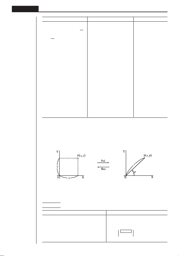
(4) Coordinate Conversion
uu
uu
u Rectangular Coordinates
uu
uu
u Polar Coordinates
•With polar coordinates,
θ
can be calculated and displayed within a range of
–180°<
θ
< 180° (radians and grads have same range).
Example To calculate r and
θ
°
when x = 14 and y = 20.7
Operation Display
!Zcc1(Deg)Q
K[2(ANGL)[[
1(Pol()14,20.7)w Ans
1
–
24.989
–
→ 24.98979792 (r)
2
–
55.928
–
→ 55.92839019 (
θ
)
7800
––––– ?
96
7800
––––– ?
96

33
Basic Calculations Chapter 2
Example To calculate x and y when r = 25 and
θ
= 56°
Operation Display
!Zcc1(Deg)Q
K[2(ANGL)[[
2(Rec()25,56)w Ans
1
–
13.979
–
→ 13.97982259 (x)
2
–
20.725
–
→ 20.72593931 (y)
(5) Permutation and Combination
uu
uu
u Permutation
uu
uu
u Combination
Example To calculate the possible number of different arrangements
using 4 items selected from 10 items
Formula Operation Display
10P4 = 5040 10K4(PROB)
2(
nPr)4w 5040
Example To calculate the possible number of different combinations of
4 items selected from 10 items
Formula Operation Display
10C4 = 210 10K4(PROB)
3(
nCr)4w 210
(6) Other Things to Remember
kk
kk
k Multiplication Sign
You can leave out the multiplication sign in any of the following cases.
•In front of the following scientific functions:
sin, cos, tan, sin
–1
, cos
–1
, tan
–1
, log, In, 10
x
, e
x
, ,
3
, Pol(x, y), Rec(r,
θ
), d/dx,
Seq, Min, Max, Mean, Median, List, Dim, Sum
Examples: 2 sin30, 10log1.2, 2
3, etc.
•In front of constants, variable names, Ans memory contents.
Examples: 2π, 2AB, 3Ans, 6X, etc.
•In front of an open parenthesis.
Examples: 3(5 + 6), (A + 1)(B –1)
n! n!
nPr = ––––– nCr = –––––––
(n – r)! r! (n – r)!

34
Chapter 2 Basic Calculations
kk
kk
k Calculation Priority Sequence
The calculation priority sequence is the order that the calculator performs opera-
tions. Note the following rules about calculation priority sequence.
•Expressions contained in parentheses are performed first.
•When two or more expressions have the same priority, they are executed from
right to left.
Example 2 + 3 × (log sin2π
2
+ 6.8) = 22.07101691 (angle unit = Rad)
The following is a complete list of operations in the sequence they are performed.
1. Coordinate transformation: (Pol (
x, y), Rec (r,
θ
); differential calculations: d/dx(;
List: Fill, Seq, Min, Max, Mean, Median, SortA, SortD
2. Type A functions (value input followed by function):
x
2
, x
–1
, x!
sexagesimal input: ° ’ ”
3. Powers: ^ (
x
y
); roots:
x
4. Fraction input: a
b
/c
5. Multiplication operations where the multiplication sign before π or a variable is
omitted: 2π; 5A; 3sin
x; etc.
6. Type B functions (function followed by value input):
,
3
, log, In, e
x
, 10
x
, sin, cos, tan, sin
–1
, cos
–1
, tan
–1
, (–), Dim, Sum
7. Multiplication operations where the multiplication sign before a scientific function
is omitted: 2
3; Alog2; etc.
8. Permutation: nPr; combination: nCr
9. Multiplication; division; integer division; remainder division
10. Addition; subtraction
11. Relational operators: =,
GG
GG
G
, >, <, ≥, ≤
kk
kk
k Using Multistatements
Multistatements are formed by connecting a number of individual statements for
sequential execution. You can use multistatements in manual calculations and in
programmed calculations. There are two different ways that you can use to connect
statements to form multistatements.
•Colon (:)
Statements that are connected with colons are executed from left to right, without
stopping.
1
2
3
4
5
6

35
Basic Calculations Chapter 2
•Display Result Command (
^^
^^
^)
When execution reaches the end of a statement followed by a display result com-
mand, execution stops and the result up to that point appears on the display. You
can resume execution by pressing the w key.
uu
uu
uTo use multistatements
Example 6.9 × 123 = 848.7
123 ÷ 3.2 = 38.4375
AbcdaaA
!W[[3(:)
g.j*aA!W[2(^)
aA/d.cw
w
•Note that the final result of a multistatement is always displayed, regardless of
whether it ends with a display result command.
•You cannot construct a multistatement in which one statement directly uses the
result of the previous statement.
Example 123 × 456: × 5
Invalid
kk
kk
k Stacks
When the calculator performs a calculation, it temporarily stores certain information
in memory areas called a “stacks” where it can later recall the information when it is
necessary.
There are actually two stacks: a 10-level numeric stack and a 26-level command
stack. The following example shows how data is stored in the stacks.
A calculation can become so complex that it requires too much stack memory and
cause a stack error (Stk ERROR) when you try to execute it. If this happens, try
simplifying your calculation or breaking it down into separate parts. See “How to
Calculate Memory Usage” for details on how much memory is taken up by various
commands.
Intermediate result at point
where “
^
” is used.
Numeric stack
Command stack
P. 3 6

36
Chapter 2 Basic Calculations
kk
kk
k Errors
An error message appears on the display and calculation stops whenever the calcu-
lator detects some problem. Press A to clear the error message.
The following is a list of all the error messages and what they mean.
Ma ERROR - (Mathematical Error)
•A value outside the range of ±9.99999999 × 10
99
was generated during a calcu-
lation, or an attempt was made to store such a value in memory.
•An attempt was made to input a value that exceeds the range of the scientific
function being used.
•An attempt was made to perform an illegal statistical operation.
Stk ERROR - (Stack Error)
• The calculation being performed caused the capacity of one of the stacks to be
exceeded.
Syn ERROR - (Syntax Error)
•An attempt to use an illegal syntax.
Arg ERROR - (Argument Error)
•An attempt to use an illegal argument with a scientific function.
Dim ERROR - (Dimension Error)
•An attempt to perform an operation with two or more lists when the dimensions of
the lists do not match.
In addition to the above, there are also a Mem ERROR and Go ERROR. See “Error
Message Table” for details.
kk
kk
k How to Calculate Memory Usage
Some key operations take up one byte of memory each, while others take up two
bytes.
1-byte operations: 1, 2, 3, ..., sin, cos, tan, log, In,
, π, etc.
2-byte operations:
d/dx(, Xmin, If, For, Return, DrawGraph, SortA(, Sum, etc.
P.200
37
Basic Calculations Chapter 2
kk
kk
k Memory Status (MEM)
You can check how much memory is used for storage for each type of data. You can
also see how many bytes of memory are still available for storage.
uu
uu
uTo check the memory status
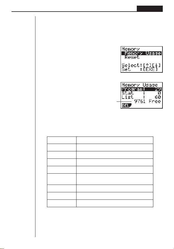
1. In the Main Menu, select the MEM icon and press w.
2. Press w again to display the memory status screen.
3. Use f and c to move the highlighting and view the amount of memory (in
bytes) used for storage of each type of data.
The following table shows all of the data types that appear on the memory status
screen.
Data type Meaning
Program Program data
Stat Statistical calculations and graphs
List List data
Y= Graph functions
Draw Graph drawing conditions (View Window,
enlargement/reduction factor, graph screen)
V-WinView Window memory data
Table Table & Graph data
Alpha Alpha memory data
kk
kk
k Clearing Memory Contents
uu
uu
uTo clear all data within a specific data type
1. In the memory status screen, use c and f to move the highlighting to the
data type whose data you want to clear.
Number of bytes still free
38
Chapter 2 Basic Calculations
2. Press 1 (DEL).
1(DEL)
3. Press 1 (YES) to clear the data or 4 (NO) to abort the operation without
clearing anything.
kk
kk
k Variable Data (VARS) Menu
You can use the variable data menu to recall the data listed below.
•View Window values
•Enlargement/reduction factor
•Single-variable/paired-variable statistical data
•Graph functions
•Table & Graph table range and table contents
To recall variable data, press J to display the variable data menu.
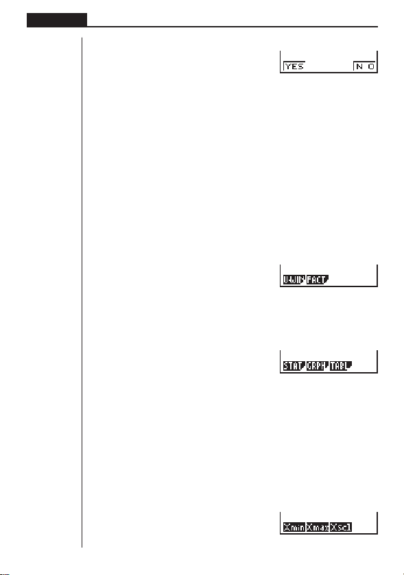
J
1 (V-WIN) .... View Window values
2 (FACT) ......
x and y-axis enlargement/reduction factor
[
1 (STAT) ...... Single/paired-variable statistical data
2 (GRPH) .... Graph functions stored in the GRAPH Mode
3 (TABL) ...... Table & Graph function table range and table contents
Press [ to return to the previous menu.
uu
uu
uTo recall View Window values
Pressing 1 (V-WIN) while the variable data menu is on the screen displays a View
Window value menu.
1 (V-WIN)
1234[
1234 [
1234 [
1 234
39
Basic Calculations Chapter 2
1 (Xmin) ....... x-axis minimum
2 (Xmax)......
x-axis maximum
3 (Xscl) ........
x-axis scale
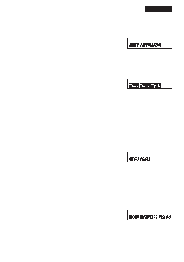
[
1 (Ymin) ....... y-axis minimum
2 (Ymax)......
y-axis maximum
3 (Yscl) ........
y-axis scale
[
1 (Tmin) ....... Minimum of T
2 (Tmax) ...... Maximum of T
3 (Tpth) ........ Pitch of T
Press [ to return to the previous menu.
uu
uu
uTo recall enlargement and reduction factors
Pressing 2 (FACT) while the variable data menu is on the screen displays an
enlargement/reduction factor menu.
2(FACT)
1 (Xfct) ......... x-axis enlargement/reduction factor
2 (Yfct) .........
y-axis enlargement/reduction factor
uu
uu
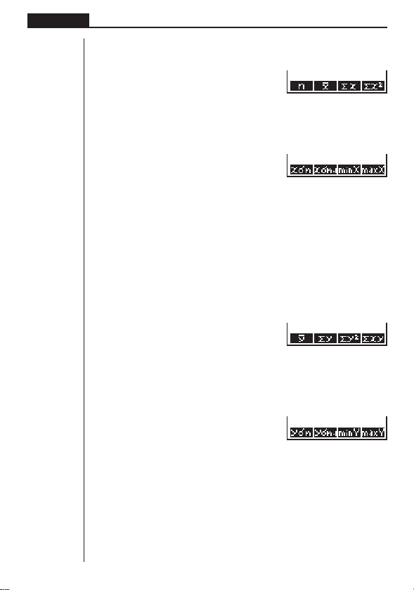
uTo recall single/paired-variable statistical data
Pressing [ and then 1 (STAT) while the variable data menu is on the screen
displays a statistical data menu.
[1(STAT)
1 (X) ............ Single/paired-variable
x-data menu
2 (Y) ............ Paired-variable
y-data menu
3 (GRPH) .... Statistical graph data menu
4 (PTS) ........ Summary point data menu
1234 [
1234 [
1234[
1234[
40
Chapter 2 Basic Calculations
The following menu appears whenever you press 1 (X), while the statistical data
menu is on the display.
1 (X)
1 (n) ............. Number of data
2 (
o) ............. Mean of x data
3 (Σ
x) ........... Sum of x data
4 (Σ
x
2
) .......... x data sum of squares
[
1 (xσn) ......... x data population standard deviation
2 (
xσn-1) ....... x data sample standard
deviation
3 (minX) .......
x data minimum value
4 (maxX)......
x data maximum value
Press [ to return to the previous menu.
The following menu appears whenever you press 2 (Y) while the statistical data
menu is on the display.
2 (Y)
1 (p) ............. Mean of y data
2 (Σ
y) ........... Sum of y data
3 (Σ
y
2
) .......... y data sum of squares
4 (Σ
xy) ......... x data and y data sum of products
[
1 (yσn) ......... y data population standard deviation
2 (
yσn-1) ....... y data sample standard deviation
3 (minY) .......
y data minimum value
4 (maxY)......
y data maximum value
Press [ to return to the previous menu.
1234[
1234[
1234[
1234[
41
Basic Calculations Chapter 2
The following menu appears whenever you press 3 (GRPH) while the statistical
data menu is on the display.
3 (GRPH)
1(a)-3(c) ... Statistical graph regression coefficient and multinomial coeffi-
cients
4 (
r) ............. Statistical graph correlation coefficient
[
1 (Q1) .......... First quartile
2 (Med) ........ Median of input data
3 (Q3) .......... Third quartile
4 (Mod) ........ Mode of input data
Press [ to return to the previous menu.
The following menu appears whenever you press 4 (PTS) while the statistical data
menu is on the display.
4 (PTS)
1(x1)-4(y2) ..... Coordinates of summary points
[
1(x3)-2(y3) ..... Coordinates of summary points
Press [ to return to the previous menu.
uu
uu
uTo recall graph functions
Pressing [ and then 2 (GRPH) while the variable data menu is on the screen
displays a graph function menu.
[2 (GRPH)
1234[
1234[
1234[
1234 [
1234[
42
Chapter 2 Basic Calculations
Input a storage area number and then press one of the following function keys to
recall the corresponding graph function stored in that storage area.
1 (Y) ............ Rectangular coordinate or inequality function
2 (Xt) ........... Parametric graph function Xt
3 (Yt) ........... Parametric graph function Yt
uu
uu
uTo recall Table & Graph table range and table content data
Pressing [ and then 3 (TABL) while the variable data menu is on the screen
displays a Table & Graph data menu.
[3(TABL)
1 (Strt) ......... Table range start value (F Start command)
2 (End) ........ Table range end value (F End command)
3 (Pitch) ....... Table value increment (F Pitch command)
1234 [

Differential Calculations
Chapter
3
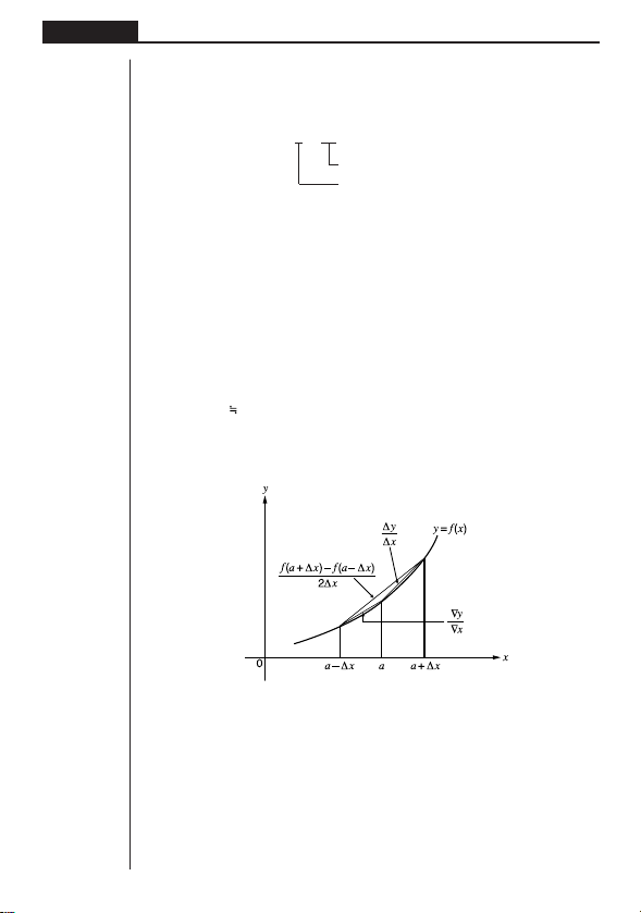
44
Chapter 3 Differential Calculations
•To perform differential calculations, first display the Option Menu, and then input
the values shown in the formula below.
K2(CALC)[
1(
d/dx) f(x),a,∆x)
The differentiation for this type of calculation is defined as:
In this definition,
infinitesimal
is replaced by a
sufficiently small
∆x, with the value in
the neighborhood of f ' (a) calculated as:
In order to provide the best precision possible, this unit employs central difference to
perform differential calculations. The following illustrates central difference.
The slopes of point a and point a + ∆x, and of point a and point a – ∆x in function
y = f(x) are as follows:
In the above, ∆
y/∆x is called the forward difference, while ∇y/∇x is the backward
difference.To calculate derivatives, the unit takes the average between the value of
∆
y/∆x and ∇y/∇x, thereby providing higher precision for derivatives.
f (a + ∆x) – f (a)
f '(a) = lim –––––––––––––
∆x
∆x→0
f (a + ∆x) – f (a) ∆y f (a) – f (a – ∆x) ∇y
––––––––––––– = ––– , ––––––––––––– = –––
∆x ∆x ∆x ∇x
f (a + ∆x ) – f (a)
f '(a)
–––––––––––––
∆x
d
d/dx ( f (x), a, ∆x) ⇒ ––– f (a)
dx
Increase/decrease of
x
Point for which you want to determine the derivative

45
Differential Calculations Chapter 3
This average, which is called the
central difference
, is expressed as:
uu
uu
uTo perform a differential calculation
Example To determine the derivative at point x = 3 for the function
y = x
3
+ 4x
2
+ x – 6, when the increase/decrease of x is defined as
∆
x = 1E – 5
Input the function
f(x).
AK2(CALC)[1(
d/dx)
TMd+eTx
+T-g,
Input point
x = a for which you want to determine the derivative.
d,
Input ∆x, which is the increase/decrease of x.
bE-f)
w
•In the function f(x), only X can be used as a variable in expressions. Other vari-
ables (A through Z) are treated as constants, and the value currently assigned to
that variable is applied during the calculation.
•Input of ∆
x and the closing parenthesis can be omitted. If you omit ∆x, the calcu-
lator automatically uses a value for ∆
x that is appropriate for the value of x = a,
which you specified as the point for which you wanted to determine the deriva-
tive.
•Discontinuous points or sections with drastic fluctuation can adversely affect pre-
cision or even cause an error.
•Note that you cannot use differential calculation inside of a differential calculation
term.
1 f (a + ∆x) – f (a) f (a) – f (a – ∆x)
f '(a) = ––
––––––––––––– + –––––––––––––
2∆x ∆x
f (a + ∆x) – f (a – ∆x)
= –––––––––––––––––
2∆x

46
Chapter 3 Differential Calculations
•Pressing A during calculation of a differential (while the cursor is not shown
on the display) interrupts the calculation.
•Always perform trigonometric differentials using radians (Rad Mode) as the
angle unit.

Graphing
A collection of versatile graphing tools plus a large 79 × 47-dot
display makes it easy to draw a variety of function graphs quickly
and easily. This calculator is capable of drawing the following types
of graphs.
•Rectangular coordinate (Y =) graphs
•Parametric graphs
•Inequality graphs
•A selection of graph commands also makes it possible to incorpo-
rate graphing into programs.
1. Before Trying to Draw a Graph
2. View Window (V-Window) Settings
3. Graph Function Operations
4. Drawing Graphs Manually
5. Other Graphing Functions
Chapter
4
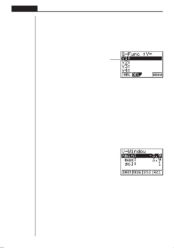
48
Chapter 4 Graphing
1. Before Trying to Draw a Graph
kk
kk
k Entering the Graph Mode
On the Main Menu, select the GRAPH icon and enter the GRAPH Mode. When you
do, the Graph Function (G-Func) menu appears on the display. You can use this
menu to store, edit, and recall functions and to draw their graphs.
1 (SEL) ........ Draw/non-draw status
2 (DEL) ........ Graph delete
4 (DRAW) .... Draws graph
2. View Window (V-Window) Settings
Use the View Window to specify the range of the x-and y-axes, and to set the spac-
ing between the increments on each axis. You should always set the View Window
parameters you want to use before drawing a graph. Press ! 3 to display the
View Window.
1. Press !3 to display the View Window.
!3(V-Window)
1 (INIT) ........ View Window initial settings
2 (TRIG) ...... View Window initial settings using specified angle unit
3 (Sto) ......... Store View Window settings to View Window memory.
4 (Rcl) .......... Recall View Window settings from View Window memory.
Xmin................ Minimum
x-axis value
Xmax............... Maximum
x-axis value
Xscl ................. Spacing of
x-axis increments
Memory area
Use
f
and
c
to change selection.
123 4
1234
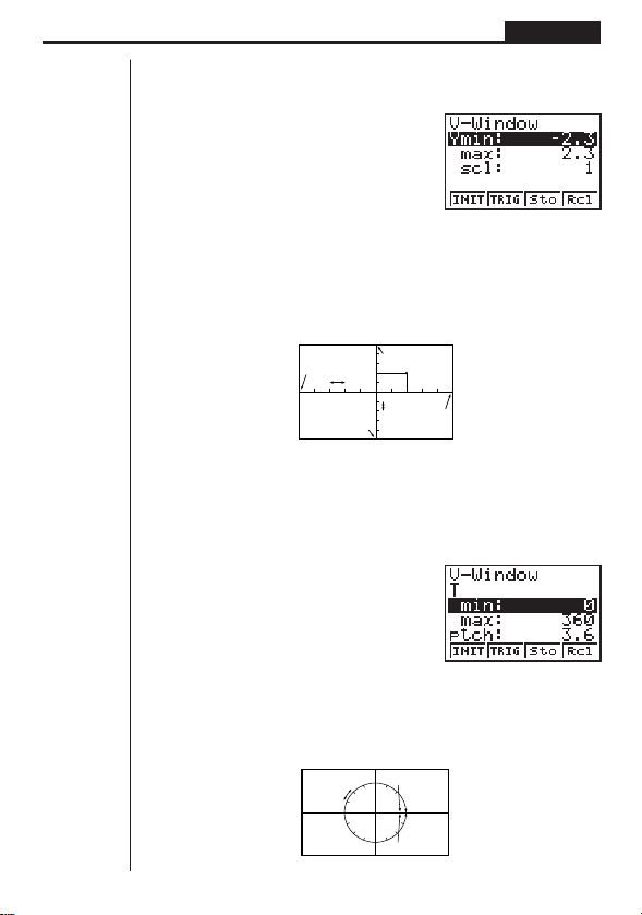
49
Graphing Chapter 4
2. Input a value for a parameter and press w. The calculator automatically selects
the next parameter for input.
•You can also select a parameter using the c and f keys.
Ymin................ Minimum y-axis value
Ymax............... Maximum
y-axis value
Yscl ................. Spacing of
y-axis increments
The following illustration shows the meaning of each of these parameters.
3. Input a value for a parameter and press w. The calculator automatically selects
the next parameter for input.
• There are actually nine View Window parameters. The remaining three param-
eters appear on the display when you move the highlighting down past the Y
scale parameter by inputting values and pressing c.
Tmin ................ T minimum values
Tmax ............... T maximum values
Tptch ............... T pitch
The following illustration shows the meaning of each of these parameters.
X max
Y scl
Y min
Y max
(x, y)
X min
X scl
min
max
ptch
(
X, Y
)

50
Chapter 4 Graphing
4. To exit the View Window, press Q.
•Pressing w without inputting any value also exits the View Window.
• The following is the input range for View Window parameters.
–9.99E+97 to 9.999E+97
•You can input parameter values up to 7 digits long. Values greater than 10
6
or
less than 10
-1
, are automatically converted to a 4-digit mantissa (including nega-
tive sign) plus a 2-digit exponent.
• The only keys that enabled while the View Window is on the display are: a to
j, ., E, -, f, c, d, e, +, -, *, /, (, ), ! 7,
Q. You can use - or - to input negative values.
• The existing value remains unchanged if you input a value outside the allow-
able range or in the case of illegal input (negative sign only without a value).
•Inputting a View Window range so the min value is greater than the max value,
causes the axis to be inverted.
•You can input expressions (such as 2π) as View Window parameters.
•When the View Window setting does not allow display of the axes, the scale for
the
y-axis is indicated on either the left or right edge of the display, while that for
the
x-axis is indicated on either the top or bottom edge.
•When View Window values are changed, the graph display is cleared and the
newly set axes only are displayed.
•View Window setting may cause irregular scale spacing.
•Setting maximum and minimum values that create too wide of a View Window
range can result in a graph made up of disconnected lines (because portions of
the graph run off the screen), or in graphs that are inaccurate.
• The point of deflection sometimes exceeds the capabilities of the display with
graphs that change drastically as they approach the point of deflection.
•Setting maximum and minimum values that create to narrow of a View Window
range can result in an error (Ma ERROR).
kk
kk
k Initializing and Standardizing the View Window
uu
uu
uTo initialize the View Window
a. Press !3 (V-Window) 1 (INIT) to initialize the View Window to the following
settings.
Xmin = –3.9 Ymin = –2.3
Xmax = 3.9 Ymax = 2.3
Xscl = 1 Yscl = 1

51
Graphing Chapter 4
b. Press ! 3 (V-Window) 2 (TRIG) to initialize the View Window to the follow-
ing settings.
Deg Mode
Xmin = –360 Ymin = –1.6
Xmax = 360 Ymax = 1.6
Xscl = 90 Yscl = 0.5
Rad Mode
Xmin = –6.28318
Xmax = 6.28318
Xscl = 1.57079
Gra Mode
Xmin = –400
Xmax = 400
Xscl = 100
• The settings for Ymin, Ymax, Ypitch, Tmin, Tmax, and Tpitch remain unchanged
when you press 2 (TRIG).
kk
kk
k View Window Memory
You can store a set of View Window settings in View Window memory for recall when
you need them.
uu
uu
uTo save View Window settings
While the View Window setting screen is on the display, press 3 (Sto) to save the
current settings.
•Whenever you save View Window settings, any settings previously stored in
memory are replaced.
uu
uu
uTo recall View Window settings
While the View Window setting screen is on the display, press 4 (Rcl) to recall the
View Window settings stored in memory.
•Whenever you recall View Window settings, the settings on the View Window are
replaced by the recalled settings.
•You can change View Window settings in a program using the following syntax.
View Window [Xmin value], [Xmax value], [Xscl value],
[Ymin value], [Ymax value], [Yscl value],
[Tmin value], [Tmax value], [Tptch value]
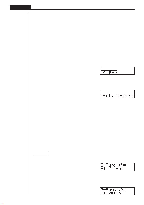
52
Chapter 4 Graphing
3. Graph Function Operations
You can store up to 10 functions in memory. Functions in memory can be edited,
recalled, and graphed. The types of functions that can be stored in memory are:
rectangular coordinate functions, parametric functions, and inequalities.
kk
kk
k Specifying the Graph Type
Before you can store a graph function in memory, you must first specify its graph
type.
1. While the Graph Function Menu is on the display, press [ to display a Graph
Type Menu.
[
1 (Y =) ......... Rectangular coordinate graph
2 (Parm) ...... Parametric graph
[
1 (Y >) ......... Y > f
(x) inequality
2 (Y <) ......... Y <
f
(x) inequality
3 (Y ≥) ......... Y >
f
(x) inequality
4 (Y ≤) ......... Y <
f
(x) inequality
Press [ to return to the previous menu
2. Press the function key that corresponds to the graph type you want to specify.
kk
kk
k Storing Graph Functions
uu
uu
uTo store a rectangular coordinate function (Y =)
Example To store the following expression in memory area Y1:
y = 2 x
2
– 5
[1(Y =)
(Specifies rectangular coordinate
expression.)
cTx-f
(Inputs expression.)
w
(Stores expression.)
1234[
1234[
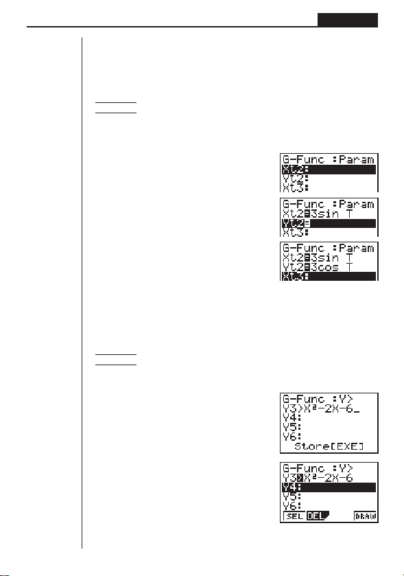
53
Graphing Chapter 4
•You will not be able to store the expression in an area that already contains a
parametric function. Select another area to store your expression or delete the
existing parametric function first. This also applies when storing inequalities.
uu
uu
uTo store a parametric function
Example To store the following functions in memory areas Xt2 and Yt2:
x = 3 sin T
y = 3 cos T
[2(Parm)
(Specifies parametric expression.)
dsTw
(Inputs and stores x expression.)
dcTw
(Inputs and stores y expression.)
•You will not be able to store the expression in an area that already contains a
rectangular coordinate expression or inequality. Select another area to store your
expression or delete the existing expression first.
uu
uu
uTo store an inequality
Example To store the following inequality in memory area Y3:
y > x
2
– 2x – 6
[[1(Y>)
(Specifies an inequality.)
Tx-cT-g
(Inputs expression.)
w
(Stores expression.)
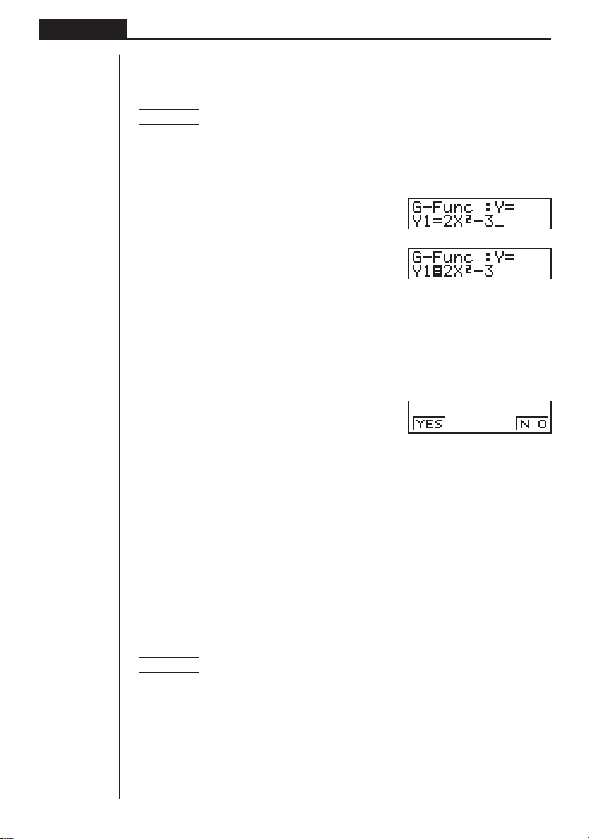
54
Chapter 4 Graphing
kk
kk
k Editing Functions in Memory
uu
uu
uTo edit a function in memory
Example To change the expression in memory area Y1 from y = 2x
2
– 5
to
y = 2x
2
– 3
e
(Displays cursor.)
eeeed
(Changes contents.)
w
(Stores new graph function.)
uu
uu
uTo delete a function
1. While the Graph Function Menu is on the display, press f or c to display the
cursor and move the highlighting to the area that contains the function you want
to delete.
2. Press 2 (DEL).
3. Press 1 (YES) to delete the function or 4 (NO) to abort the procedure without
deleting anything.
kk
kk
k Drawing a Graph
Before actually drawing a graph, you should first make the draw/non-draw status.
uu
uu
uTo specify the draw/non-draw status of a graph
You can specify which functions out of those stored in memory should be used for a
draw operation.
•Graphs for which there is no draw/non-draw status specification are not drawn.
Example To select the following functions for drawing:
Y1 :
y = 2x
2
– 5
X
t2: x = 3 sin T
Y
t2: y = 3 cos T
1 234
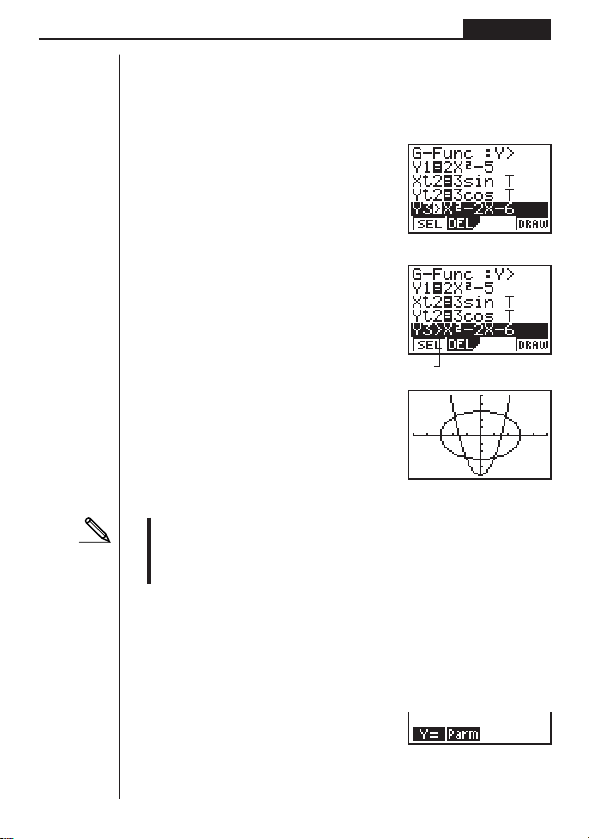
55
Graphing Chapter 4
Use the following View Window parameters.
Xmin = –5 Ymin = –5
Xmax = 5 Ymax = 5
Xscl = 1 Yscl = 1
ccc
(Select a memory area that contains a
function for which you want to specify
non-draw.)
1(SEL)
(Specify non-draw.)
4(DRAW) or w
(Draws the graphs.)
•Pressing u or A returns to the Graph Function Menu.
•A parametric graph will appear coarse if the settings you make in the View
Window cause the pitch value to be too large, relative to the differential be-
tween the min and max settings. If the settings you make cause the pitch value
to be too small relative to the differential between the min and max settings, on
the other hand, the graph will take a very long time to draw.
4. Drawing Graphs Manually
After you select the RUN icon in the Main Menu and enter the RUN Mode, you can
draw graphs manually. First press ! 4 (SKTCH) 2 (GRPH) to recall the Graph
Command Menu, and then input the graph function.
!4(SKTCH)2(GRPH)
1 (Y =) ......... Rectangular coordinate graph
2(Parm) ....... Parametric graph
1 234
1234
1234[
Unhighlights
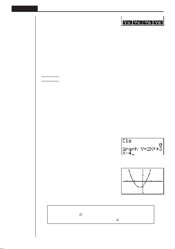
56
Chapter 4 Graphing
[
1 (Y >) ......... Y > f
(x) inequality
2 (Y <) ......... Y <
f
(x) inequality
3 (Y ≥) ......... Y >
f
(x) inequality
4 (Y ≤) ......... Y <
f
(x) inequality
Press [ to return to the previous menu.
uu
uu
uTo graph using rectangular coordinates (Y =)
You can graph functions that can be expressed in the format y = f(x).
Example To graph y = 2x
2
+ 3x – 4
Use the following View Window parameters.
Xmin = –5 Ymin = –10
Xmax = 5 Ymax = 10
Xscl = 2 Yscl = 5
1. In the set-up screen, specify the appropriate graph type for F-Type.
!Z1(Y =)Q
2. Input the rectangular coordinate (Y =) expression.
A!4(SKTCH)1(Cls)w
2(GRPH)1(Y =)
cTx+dT-e
3. Press w to draw the graph.
w
•You can draw graphs of the following built-in scientific functions.
• sin x • cos x • tan x • sin
–1
x • cos
–1
x
• tan
–1
x • • x
2
• log x • lnx
• 10
x
• e
x
• x
–1
•
3
View Window settings are made automatically for built-in graphs.
1234[
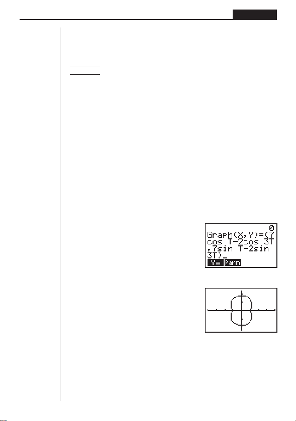
57
Graphing Chapter 4
uu
uu
uTo graph parametric functions
You can graph parametric functions that can be expressed in the following format.
(X, Y) = (
f (T), g(T))
Example To graph the following parametric functions:
x = 7 cos T – 2 cos 3T
y = 7 sin T – 2 sin 3T
Use the following View Window parameters.
Xmin = –20 Ymin = –12
Xmax = 20 Ymax = 12
Xscl = 5 Yscl = 5
Tmin = 0 Tmax = 2π
Tptch = π÷36
1. In the set-up screen, specify the appropriate graph type for F-Type.
!Z2(Parm)
2. Set the default angle unit to radians (Rad).
cc2(Rad)Q
3. Input the parametric functions.
A!4(SKTCH)1(Cls)w
2(GRPH)2(Parm)
hcT-ccdT,
hsT-csdT)
4. Press w to draw the graph.
w
uu
uu
uTo graph inequalities
You can graph inequalities that can be expressed in the following four formats.
•
y > f
(x)
•
y < f
(x)
•
y > f
(x)
•
y < f
(x)
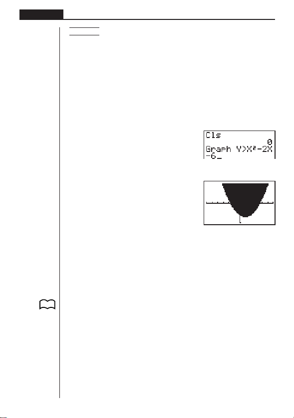
58
Chapter 4 Graphing
Example To graph the inequality y > x
2
– 2x – 6
Use the following View Window parameters.
Xmin = –6 Ymin = –10
Xmax = 6 Ymax = 10
Xscl = 1 Yscl = 5
1. In the set-up screen, specify the appropriate graph type for F-Type.
!Z[1(Y>)Q
2. Input the inequality.
A!4(SKTCH)1(Cls)w
2(GRPH)[1(Y>)
Tx-cT-g
3. Press w to draw the graph.
w
5. Other Graphing Functions
The functions described in this section tell you how to read the x- and y-coordinates
at a given point, and how to zoom in and zoom out on a graph.
• These functions can be used with rectangular coordinate, parametric, and in-
equality graphs only.
kk
kk
k Connect Type and Plot Type Graphs (D-Type)
You can use the D-Type setting of the set-up screen to specify one of two graph
types.
•Connect type (Conct)
Points are plotted and connected by lines to create a curve.
•Plot
Points are plotted without being connected.
P. 7
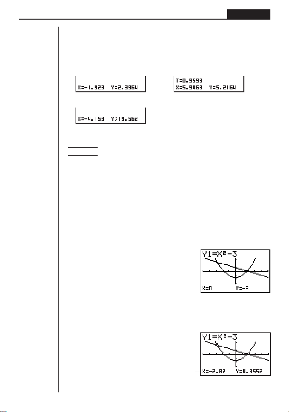
59
Graphing Chapter 4
kk
kk
k Trace
With trace, you can move a flashing pointer along a graph with the f, c, d, and
e cursor keys and obtain readouts of coordinates at each point. The following
shows the different types of coordinate readouts produced by trace.
•Rectangular Coordinate Graph • Parametric Function Graph
•Inequality Graph
uu
uu
uTo use trace to read coordinates
Example To determine the points of intersection for graphs produced by
the following functions:
Y1:
y = x
2
– 3
Y2:
y = –x + 2
Use the following View Window parameters.
Xmin = –5 Ymin = –10
Xmax = 5 Ymax = 10
Xscl = 1 Yscl = 2
1. After drawing the graphs, press 1 (TRCE) to display the pointer in the center of
the graph.
1(TRCE)
• The pointer may not be visible on the graph when you press 1 (TRCE).
2. Use d to move the pointer to the first intersection.
d
~ d
x/y
coordinate values
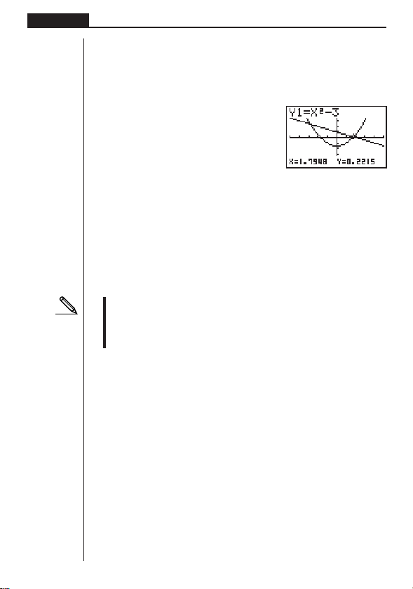
60
Chapter 4 Graphing
•Pressing d and e moves the pointer along the graph. Holding down either
key moves the pointer at high speed.
3. Use f and c to move the pointer between the two graphs.
4. Use e to move the pointer to the other intersection.
e
~ e
•To quit the trace operation, press 1 (TRCE) again.
uu
uu
uScrolling
When the graph you are tracing runs off the display along either the x- or y-axis,
pressing the e or d cursor key causes the screen to scroll in the corresponding
direction eight dots.
•You can scroll only rectangular coordinate and inequality graphs while tracing.
You cannot scroll parametric function graphs.
•Trace can be used only immediately after a graph is drawn. It cannot be used
after changing the settings of a graph.
•You cannot incorporate trace into a program.
•You can use trace on a graph that was drawn as the result of an output com-
mand (^), which is indicated by the “-Disp-” indicator on the screen.
kk
kk
k Scroll
You can scroll a graph along its x- or y-axis. Each time you press f, c, d, or
e, the graph scrolls 12 dots in the corresponding direction.
kk
kk
k Overwrite
Using the following syntax to input a graph causes multiple versions of the graph to
be drawn using the specified values. All versions of the graph appear on the display
at the same time.
<function with one variable> , ! [ <variable name> ! =
<value> , <value> , .... <value> ! ] w
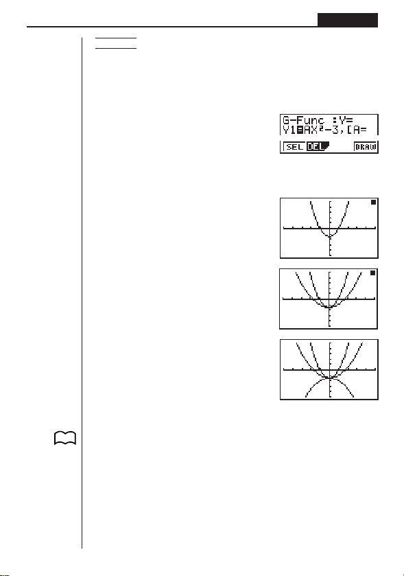
61
Graphing Chapter 4
Example To graph y = Ax
2
– 3, substituting 3, 1, and –1 for the value of A
Use the following View Window parameters.
Xmin = –5 Ymin = –10
Xmax = 5 Ymax = 10
Xscl = 1 Yscl = 2
[1(Y =)
(Specifies graph type.)
aATx-d,
![aA!=d,
b,-b!]w
(Stores expression.)
4(DRAW) or w
(Draws graph.)
↓
↓
• The function that is input using the above syntax can have only one variable.
•You cannot use X, Y or T as the variable name.
•You cannot assign a variable to the variable in the function.
•When the set-up screen’s Simul-G item is set to “On,” the graphs for all the vari-
ables are drawn simultaneously.
1234
P. 8

62
Chapter 4 Graphing
kk
kk
k Zoom
The zoom feature lets you enlarge and reduce a graph on the display.
uu
uu
uBefore using zoom
Immediately after drawing a graph, press !2 (ZOOM) to display the Zoom Menu.
!2(ZOOM)
1 (BOX) ....... Graph enlargement using box zoom
2 (FACT) ...... Displays screen for specification of zoom factors
3 (IN) ........... Enlarges graph using zoom factors
4 (OUT) ....... Reduces graph using zoom factors
[
1 (ORIG)...... Original size
Press [ to return to the previous menu
uu
uu
uTo use box zoom
With box zoom, you draw a box on the display to specify a portion of the graph, and
then enlarge the contents of the box.
Example To use box zoom to enlarge a portion of the graph y = (x + 5)
(
x + 4) (x + 3)
Use the following View Window parameters.
Xmin = –8 Ymin = –4
Xmax = 8 Ymax = 2
Xscl = 2 Yscl = 1
1. After graphing the function, press !2 (ZOOM).
!2(ZOOM)
1234[
1 234[
1 234
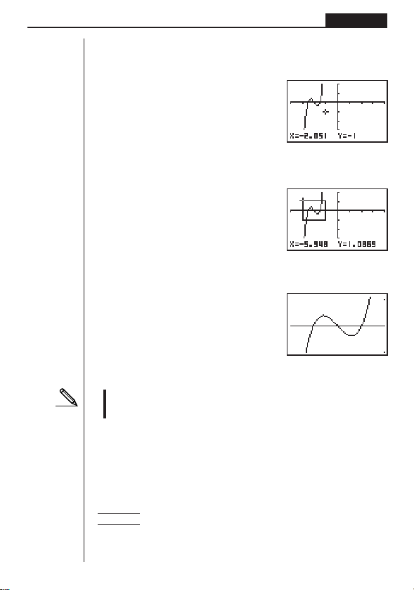
63
Graphing Chapter 4
2. Press 1 (BOX), and then use the cursor keys (d, e, f, c) to move the
pointer to the location of one of the corners of the box you want to draw on the
screen. Press w to specify the location of the corner.
1(BOX)
d ~ dw
3. Use the cursor keys to move the pointer to the location of the corner that is diago-
nally across from the first corner.
f
~ f d ~ d
4. Press w to specify the location of the second corner. When you do, the part of
the graph inside the box is immediately enlarged so it fills the entire screen.
w
•To return to the original graph, press 2 (ZOOM) [ 1 (ORIG).
•Nothing happens if you try to locate the second corner at the same location or
directly above the first corner.
•You can use box zoom for any type of graph.
uu
uu
uTo use factor zoom
With factor zoom, you can zoom in or zoom out on the display, with the current
pointer location being at the center of the new display.
•Use the cursor keys (d, e, f, c) to move the pointer around the display.
Example Graph the two functions below, and enlarge them five times in
order to determine whether or not they are tangential:
Y1:
y = (x + 4) (x + 1) (x – 3)
Y2:
y = 3x + 22
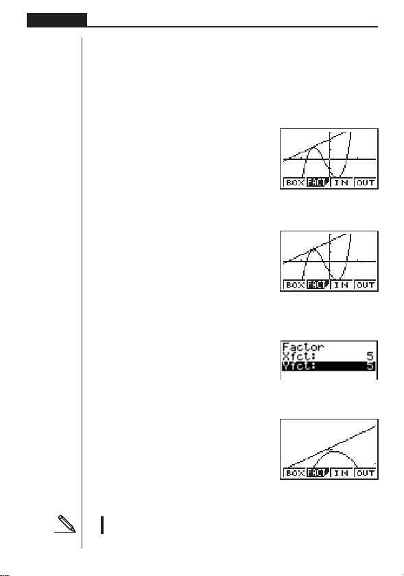
64
Chapter 4 Graphing
Use the following View Window parameters.
Xmin = –8 Ymin = –30
Xmax = 8 Ymax = 30
Xscl = 5 Yscl = 10
1. After graphing the functions, press !2 (ZOOM), and the pointer appears on
the screen.
!2(ZOOM)
2. Use the cursor keys (d, e, f, c) to move the pointer to the location that
you want to be the center of the new display.
d
~ d f ~ f
3. Press 2 (FACT) to display the factor specification screen, and input the factor
for the
x- and y-axes.
2(FACT)
fwfw
4. Press Q to return to the graphs, and then press 3 (IN) to enlarge them.
Q3(IN)
This enlarged screen makes it clear that the graphs of the two expressions are not
tangential.
•Note that the above procedure can also be used to reduce the size of a graph
(zoom out). In step 4, press 4 (OUT).
1 2 34
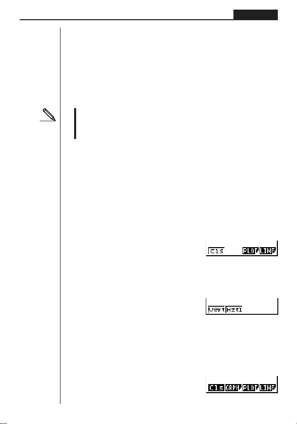
65
Graphing Chapter 4
1 2 34[
1234[
1234[
• The above procedure automatically converts the
x-range and y-range View Win-
dow values to 1/5 of their original settings.
•You can repeat the factor zoom procedure more than once to further enlarge or
reduce the graph.
uu
uu
uTo initialize the zoom factor
Press !
2 (ZOOM) 2 (FACT) 1 (INIT) to initialize the zoom factor to the
following settings.
Xfct = 2 Yfct = 2
•You can use the following syntax to incorporate a factor zoom operation into a
program.
Factor <X factor>, <Y factor>
•You can use factor zoom for any type of graph.
kk
kk
k Sketch Function
The sketch function lets you draw lines and graphs on an existing graph.
•Note that Sketch function operation in the STAT, GRAPH or TABLE Mode is
different from Sketch function operation in the RUN or PRGM Mode.
uu
uu
uBefore using the Sketch Function
Press ! 4 (SKTCH) to display the sketch menu.
In the STAT, GRAPH or TABLE Mode
!4(SKTCH)
1 (Cls) .......... Clears drawn line and point
3 (PLOT)...... Displays plot menu
4 (LINE) ....... Displays line menu
[
1 (Vert) ........ Vertical line
2 (Hztl) ......... Horizontal line
Press [ to return to the previous menu
In the RUN or PRGM Mode
!4(SKTCH)

66
Chapter 4 Graphing
[
•Other menu items are identical to those in the STAT, GRAPH, TABLE Mode menu.
The Sketch function lets you draw lines and plot points on a graph that is already on
the screen.
All the examples in this section that show operations in the STAT, GRAPH or TABLE
Mode are based on the assumption that the following function has already been
graphed in the GRAPH Mode.
Memory Area Y1:
y = x(x + 2)(x – 2)
The following are the View Window parameters used when drawing the graph.
Xmin = –5 Ymin = –5
Xmax = 5 Ymax = 5
Xscl = 1 Yscl = 1
uu
uu
uTo plot points
In the STAT, GRAPH or TABLE Mode
Example To plot a point on the graph of y = x(x + 2)(x – 2)
1. After graphing the function, display the sketch menu and perform the following
operation to cause the pointer to appear on the graph screen.
!4(SKTCH)3(PLOT)1(Plot)
2. Use the cursor keys (f, c, d, e) to move the pointer the locations of the
points you want to plot and press w to plot.
•You can plot as many points as you want.
e ~ ef ~ f
w
•The current x- and y-coordinate values are assigned respectively to variables X
and Y.
1234
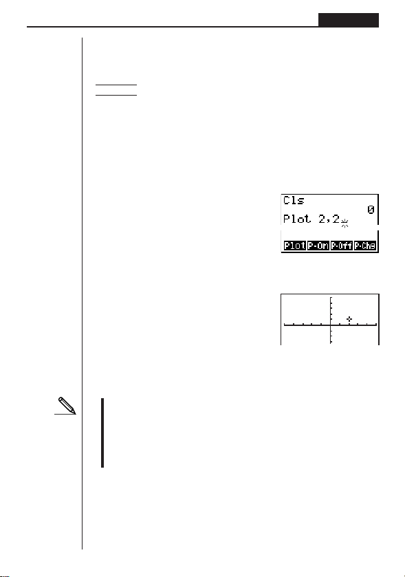
67
Graphing Chapter 4
In the RUN or PRGM Mode
The following is the syntax for plotting points in these modes.
Plot <
x-coordinate>, <y-coordinate>
Example To plot a point at (2, 2)
Use the following View Window parameters.
Xmin = –5 Ymin = –10
Xmax = 5 Ymax = 10
Xscl = 1 Yscl = 2
1. After entering the RUN Mode, display the sketch menu and perform the following
operation.
!4(SKTCH)1(Cls)w
3(PLOT)1(Plot)c,c
2. Press w.
ww
•You can use the cursor keys (f, c, d, e) to move the pointer around the
screen.
• If you do not specify coordinates, the pointer is located in the center of the
graph screen when it appears on the display.
• If the coordinates you specify are outside the range of the View Window param-
eters, the pointer will not be on the graph screen when it appears on the dis-
play.
•The current
x- and y-coordinate values are assigned respectively to variables X
and Y.

68
Chapter 4 Graphing
uu
uu
uTo turn plot points on and off in the STAT, GRAPH and TABLE Modes
• To turn a plot point on
1. After drawing a graph, display the sketch menu and then perform the following
operation to make the pointer appear at the center of the screen.
!4(SKTCH)3(PLOT)2(P-On)
2. Use the cursor keys (f, c, d, e) to move the pointer to the location where
you want to plot a point and then press w.
• To turn a plot point off
Perform the same procedure as described under “To turn a plot point on” above,
except press 3 (P-Off) in place of 2 (P-On).
• To change the on/off status of a plot point
Perform the same procedure as described under “To turn a plot point on” above,
except press 4 (P-Chg) in place of 2 (P-On).
uu
uu
uTo turn plot points on and off in the RUN or PRGM Mode
The following are the syntax for turning plot points on and off in these modes.
• To turn a plot point on
PlotOn <
x-coordinate>, <y-coordinate>
• To turn a plot point off
PlotOff <
x-coordinate>, <y-coordinate>
• To change the on/off status of a plot point
PlotChg <
x-coordinate>, <y-coordinate>
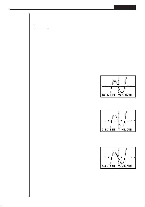
69
Graphing Chapter 4
uu
uu
uTo draw a line between two plotted points
In the STAT, GRAPH or TABLE Mode
Example To draw a line between the two points of inflection on the graph
of
y = x(x + 2)(x – 2)
Use the same View Window parameters as in the example on page
66.
1. After graphing the function, display the sketch menu and perform the following
operation to cause the pointer to appear on the graph screen.
!4(SKTCH)3(PLOT)1(Plot)
2. Use the cursor keys (f, c, d, e) to move the pointer to one of the points of
inflection and press w to plot it.
d ~ df ~ f
w
3. Use the cursor keys to move the pointer to the other point of inflection.
e ~ ec ~ c
4. Display the sketch menu and perform the following operation to draw a line be-
tween the two points.
!4(SKTCH)4(LINE)1(Line)
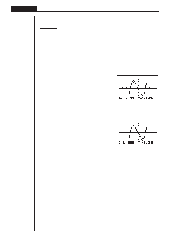
70
Chapter 4 Graphing
uu
uu
uTo draw a line in the STAT, GRAPH and TABLE Modes
Example To draw a line between two points of inflection on the graph of
y = x(x + 2)(x – 2)
1. After graphing the function, display the sketch menu and perform the following
operation to cause the pointer to appear on the graph screen.
!4(SKTCH)4(LINE)2(F-Lin)
2. Use the cursor keys (f, c, d, e) to move the pointer to one of the points of
inflection and press w.
d ~ df ~ f
w
3. Use the cursor keys to move the pointer to the other point of inflection and press
w to draw the line.
e ~ ec ~ c
w
uu
uu
uTo draw a line in the RUN or PRGM Mode
The following is the syntax for drawing lines in these modes.
F-Line <
x-coordinate 1>, <y-coordinate 1>, <x-coordinate 2>, <y-coordinate 2>
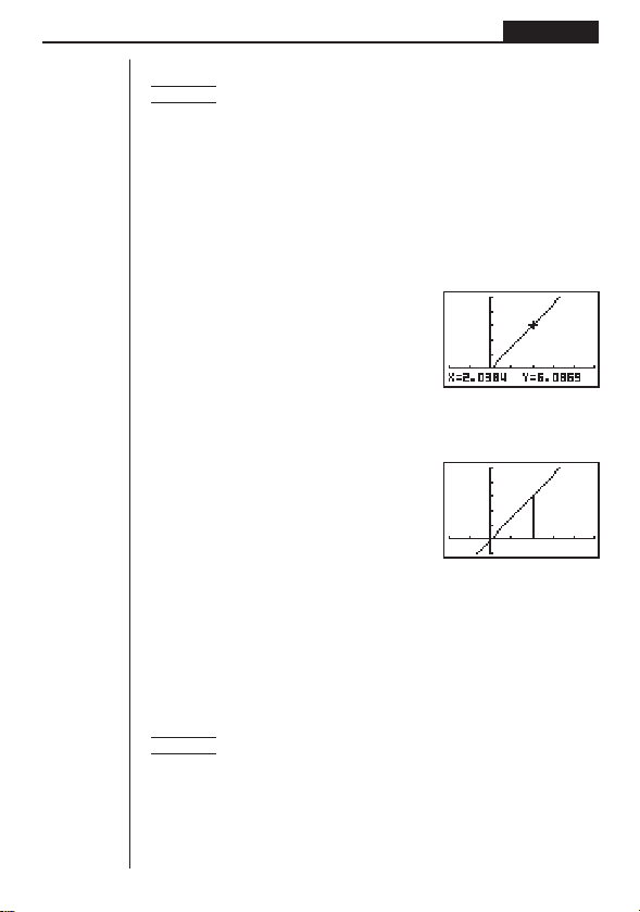
71
Graphing Chapter 4
In the RUN or PRGM Mode
Example To draw a line perpendicular to the x-axis from point (x, y) = (2, 6)
on the graph
y = 3x
Use the following View Window parameters:
Xmin = –2 Ymin = –2
Xmax = 5 Ymax = 10
Xscl = 1 Yscl = 2
1. After drawing the graph, use the procedure under “To plot points” to move the
pointer to (
x, y) = (2, 0), then use the cursor key (f) to move the pointer on the
graph
y = 3x.
u
!4(SKTCH)3(PLOT)1(Plot)
c,awwf~f
2. Display the sketch menu and perform the following operation to draw a straight
line between the two points.
u
!4(SKTCH)4(LINE)1(Line)w
• The above draws a straight line between the current pointer location and the
previous pointer location.
uu
uu
uTo draw vertical and horizontal lines
The procedures presented here draw vertical and horizontal lines that pass through
a specific coordinate.
In the STAT, GRAPH or TABLE Mode
Example To draw a vertical line on the graph of y = x(x + 2)(x – 2)
1. After graphing the function, display the sketch menu and perform the following
operation to display the pointer and draw a vertical line through its current loca-
tion.
!4(SKTCH)[1(Vert)
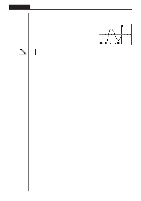
72
Chapter 4 Graphing
2. Use the d and e cursor keys to move the line left and right, and press w to
draw the line at the current location.
e ~ ew
•To draw a horizontal line, simply press 2 (Hztl) in place of 1 (Vert), and use
the f and c cursor keys to move the horizontal line on the display.
In the RUN or PRGM Mode
The following is the syntax for drawing vertical and horizontal lines in these modes.
• To draw a vertical line
Vertical <
x-coordinate>
• To draw a horizontal line
Horizontal <
y-coordinate>
uu
uu
uTo clear drawn lines and points
The following operation clears all drawn lines and points from the screen.
In the STAT, GRAPH or TABLE Mode
Lines and points drawn using sketch menu functions are temporary. Display the
sketch menu and press 1 (Cls) to clear drawn lines and points, leaving only the
original graph.
In the RUN or PRGM Mode
The following is the syntax for clearing drawn lines and points, as well as the graph
itself.
Cls

Table & Graph
The Table & Graph menu makes it possible to generate numeric
tables from functions stored in memory. You can also use multiple
functions to generate tables. Since Table & Graph uses the same
list of functions that the GRAPH Mode uses for graphing, there is
no need to input the same functions in different modes.
•You can specify the range and increment of values assigned to
variables for table value generation.
•You can assign list values to variables.
•In addition to graphing of stored functions, you can also plot table
values generated by Table & Graph itself.
•Table values can be assigned to a list.
1. Storing a Function
2. Deleting a Function
3. Assigning Values to a Variable
4. Generating a Numeric Table
5. Editing a Table
6. Graphing a Function
7. Assigning Numeric Table Contents to a List
Chapter
5
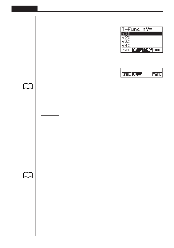
74
Chapter 5 Table and Graph
To enter the Table Mode, press m to display the Main Menu, use the cursor keys to
select the TABLE icon, and then press w.
This is the initial Table Mode screen. To generate a table, you must first specify the
variable range.
The menu at the bottom of the display looks like the one shown here when the Var
item of the set-up screen is set to a list name (indicating that variable values should
be obtained from a list).
1. Storing a Function
Example To store the function y = 3 x
2
– 2 in memory area Y1
Use f and c to move the highlighting in the TABLE Mode function list to the
memory area where you want to store the function. Next, input the function and
press w to store it.
2. Deleting a Function
Use f and c to move the highlighting to the memory area that contains the
function you want to delete.
Press 2 (DEL).
Press 1 (YES) to delete the selected function or 4 (NO) to abort the delete
operation without deleting anything.
The procedures for storing and deleting functions are identical to those used in the
GRAPH Mode.
3. Assigning Values to a Variable
You can use either one of two methods to assign values to a variable: automatic
assignment within a specified range, and assignment of values from a list. The stand-
ard default method is automatic assignment within a specified range.
P. 5 2
P. 8
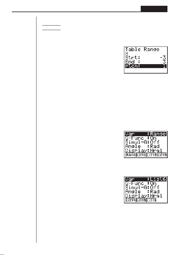
75
Table and Graph Chapter 5
uu
uu
uTo assign values automatically within a specified range
ExampleTo assign values from –3 to 3, in increments of 1 (seven values
total)
3(RANG)
-dwdwbw
Strt: ................. Variable x start value
End: ................ Variable x end value
ptch: ................ Variable x value change
To interrupt automatic assignment of variables and return to the function storage
screen, press Q.
uu
uu
uTo assign values from a list
Press ! Z to display the set-up screen.
!Z
If necessary, you can press [ to display a menu of other lists (4, 5, 6). The follow-
ing shows the operation required to select List 6.
[3(List6)
After making the set-up screen setting you want, press Q to return to the Function
List. Note that the [RANG] item does not appear in the function key menu at the
bottom of the screen when a list is selected for assignment of variable values.
123 4
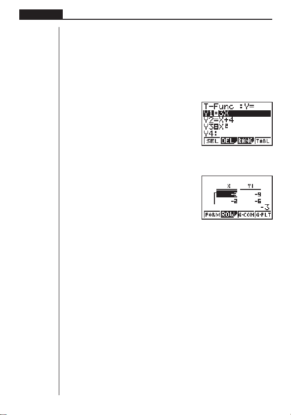
76
Chapter 5 Table and Graph
4. Generating a Numeric Table
Before actually generating a numeric table, you must first select the functions you
want to use.
Use the f and c cursor keys to move the highlighting to the function you want to
use and then press 1 (SEL) to select it.
The “=” symbols of selected functions are highlighted on the display. You can select
more than one function for table generation.
In this display, Y1 and Y3 are selected.
Press 4 (TABL) or w to generate a numeric table.
•In this example, values are assigned automatically.
This display shows the generated numeric table. Though this example display shows
only the values for function Y1, values for function Y3 were also generated.
Each cell can hold up to six digits (negative sign takes up one digit).
You can move the cursor around the table using the cursor (f, c, d, e) keys.
The following points apply to cursor position and movement.
• The value contained in the currently selected cell appears at the bottom of the
display, with all current display attributes (number of decimal place, number of
significant digit, and exponential display range settings) applied.
•Moving the cursor off the screen causes the table to scroll when there are cells
off the top, bottom, left, or right .
•When the cursor is located in any function value cell (Y1, Y2, etc.), the function is
shown at the top of the display.
• If you change a value in column X, the corresponding function value is automati-
cally updated using the new value for X.
To return to the Function List, press 1 (FORM).
1234
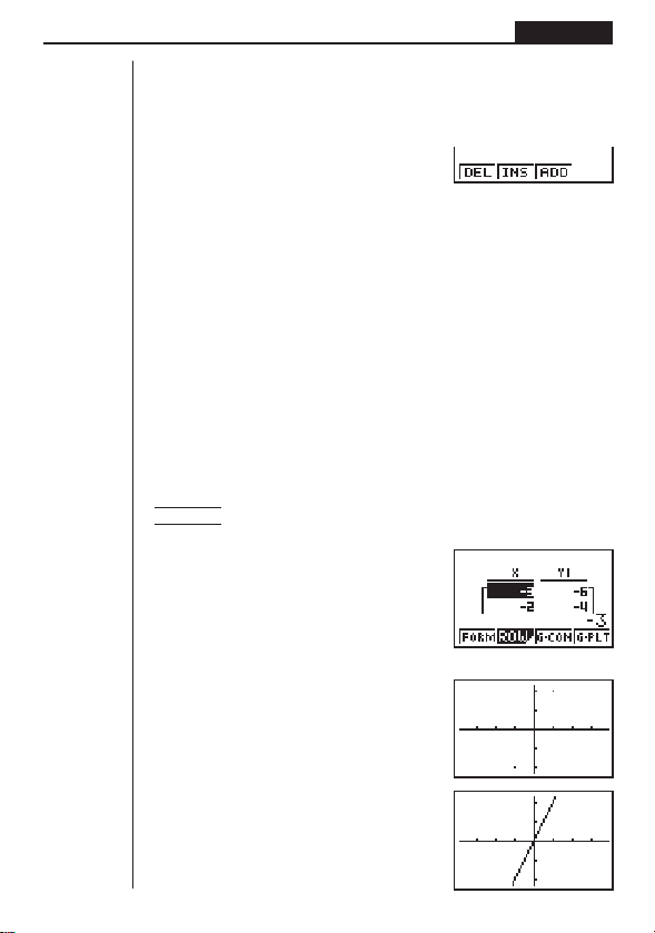
77
Table and Graph Chapter 5
1234
1234
5. Editing a Table
You can use the editing screen to add lines to or delete lines from an existing table.
Press 2 (ROW) to display the Table Editing Menu.
2(ROW)
1 (DEL) ........ Deletes line where cursor is located.
2 (INS) ......... Inserts new line where cursor is located.
3 (ADD) ....... Insert new line below line where cursor is located.
6. Graphing a Function
You can use the two following function keys to produce a graph using the numeric
table currently on the screen.
3 (G-CON) ... Graph with connected plot points
4 (G-PLT) ..... Graph with plotted points (unconnected)
•Note that you can also produce a G-PLT (4) graph by pressing w while a
numeric table is on the screen.
Example To graph the function Y1 = 2X, whose table of numeric values is
currently on the screen
4(G-PLT)
3(G-CON)
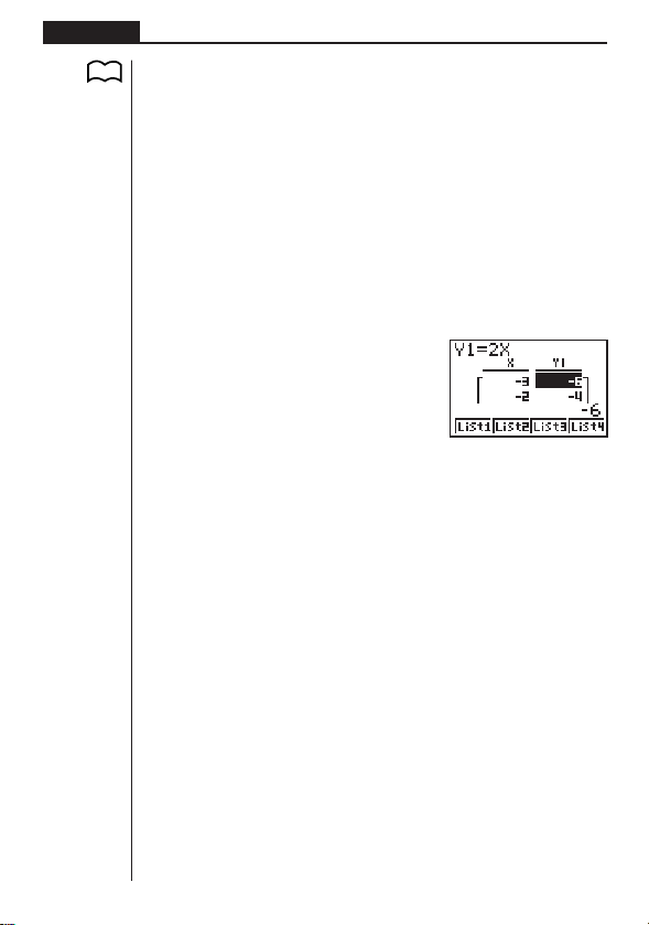
78
Chapter 5 Table and Graph
Graphing a table whose values were generated using more than one function causes
the graphs of all the functions to be drawn at the same time. You can set
x- and y-
axis parameters using the View Window.
Press u or A to return to the numeric table screen from a graph. Pressing u
again goes back to the graph. You can use u to switch between the graph and its
table as long as you do not clear the graph.
7. Assigning Numeric Table Contents to
a List
You can assign a column of values from a table into a list. Simply use d and e to
move the cursor into the column whose values you want to copy. The cursor can be
in any row of the column. The copy operation is performed by pressing K to dis-
play the Option Menu, and then pressing 2 (LMEM).
K1(LIST)2(LMEM)
Use the first function menu to copy the column’s values to List 1 (1) to List 4 (4).
To copy to List 5 or List 6, press [ and then 1 (List 5) or 2 (List 6).
P. 4 8
1234[
List Function
A list is a kind of container that you can use to store multiple data items.
This calculator lets you have up to six lists in memory, and their
contents can be used in arithmetic calculations, statistical calcula-
tions and for graphing.
1. List Operations
2. Editing and Rearranging Lists
3. Manipulating List Data
4. Arithmetic Calculations Using Lists
6
Chapter
Element number Display range Cell
List name
Column
List 1 List 2 List 3 List 4 List 5 List 6
156 1107 3.5 40
237 275 6 00
321 4122 2.1 00
469 887 4.4 20
540 16298 3 00
648 3248 6.8 30
793 64338 2 90
830 12849 8.7 00
••••••
••••••
••••••
••••••
Row
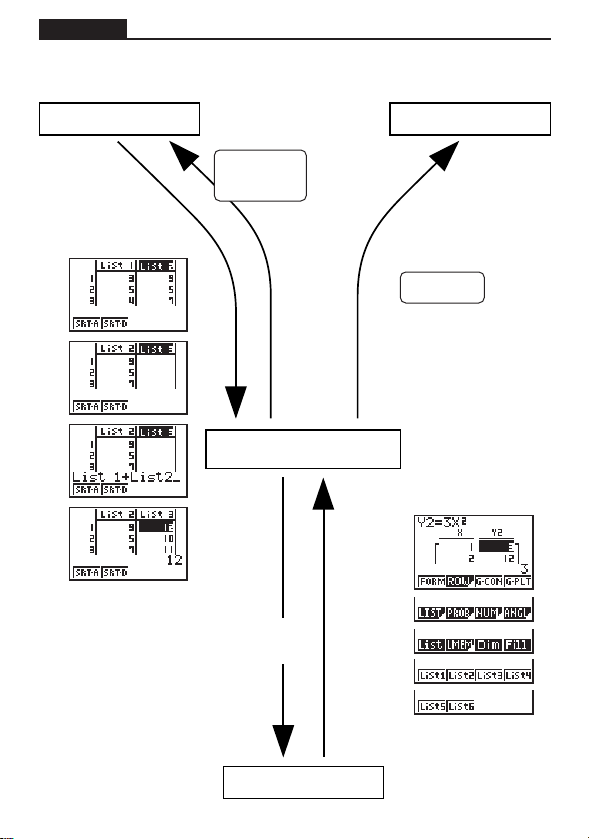
kk
kk
k List Data Linking
80
List operation
Example:
List 1 + List 2
{1, 2, 3} + {4, 5, 6}
List 1 + 3
GraphOperation
List internal operations
a
w
Graphing with
list data
Example:
Y1=List 1X
Table
LIST
Copying table result to a list
K
1(LIST)
2(LMEM)
Specific selected data can
be copied to a list.
List data can be assigned to a
variable for generation of a table
(defined using set-up screen).
Chapter 6 List Function
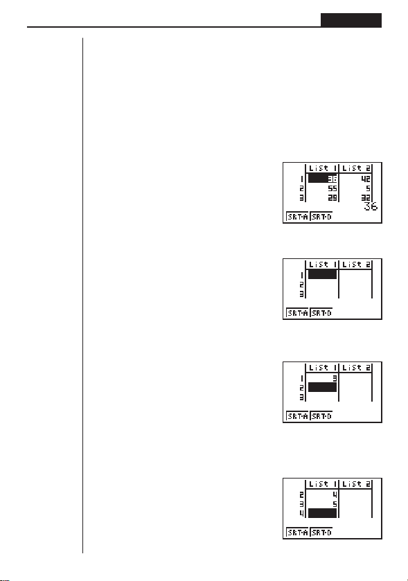
81
List Function Chapter 6
1. List Operations
Select the LIST icon in the Main Menu and enter the LIST Mode to input data into a
list and to manipulate list data.
uu
uu
uTo input values one-by-one
Use d and e to move between lists, and f and c to move between cells
inside of a list.
The screen automatically scrolls when the cursor is located at the edge of the screen.
For our example, we will start by locating the cursor in Cell 1 of List 1.
1. Input a value and press w to store it in the list.
dw
2. The cursor automatically moves down to the next cell for input.
Let’s continue our example by inputting the values 4 and 5.
ewfw
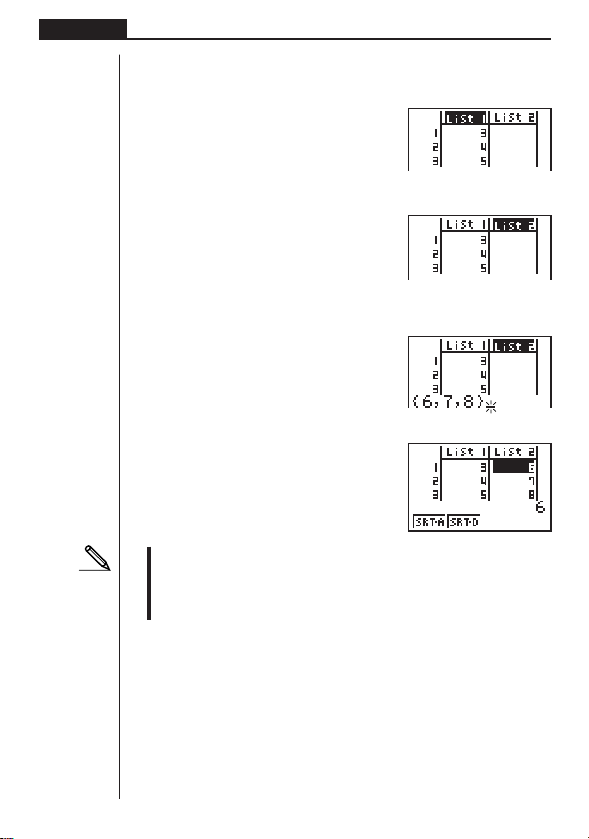
82
Chapter 6 List Function
uu
uu
uTo batch input a series of values
1. Use f to move the cursor to the list name.
ffff
2. Use d or e to move the cursor to another list.
e
3. Press !{, and then input the values you want, pressing , between each
one. Press !} after inputting the final value.
!{g,h,i!}
4. Press w to store all of the values in your list.
w
•Remember that a comma separates values, so you should not input a comma
after the final value of the set you are inputting.
Right: {34, 53, 78}
Wrong: {34, 53, 78,}
2. Editing and Rearranging Lists
kk
kk
k Editing List Values
uu
uu
uTo change a cell value
Use d or e to move the cursor to the cell whose value you want to change. Input
the new value and press w to replace the old data with the new one.
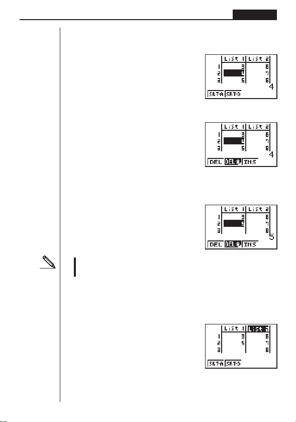
83
List Function Chapter 6
uu
uu
uTo delete a cell
1. Use d, e, f, or c to move the cursor to the cell you want to delete.
cd
2. Press [ to display the Cell Operation Menu.
[
3. Press 1 (DEL) to delete the selected cell and cause everything below it to be
shifted up.
1(DEL)
•Note that the above cell delete operation does not affect cells in other lists. If
the data in the list whose cell you delete is somehow related to the data in
neighboring lists, deleting a cell can cause related values to become misaligned.
uu
uu
uTo delete all cells in a list
1. Use d, e, f or c to move the cursor to the name of the list whose cells
you want to delete.
1 234
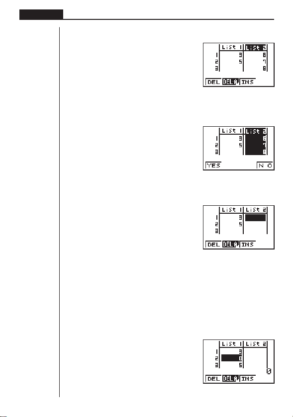
84
Chapter 6 List Function
2. Press [ to display the Cell Operation Menu (if it is not already displayed).
[
3. Press 2 (DEL-A). The function menu changes to confirm whether you really
want to delete all the cells in the list.
2(DEL-A)
4. Press 1 (YES) to delete all the cells in the selected list or 4 (NO) to abort the
delete operation without deleting anything.
1(YES)
uu
uu
uTo insert a new cell
Use d, e, f, or c to move the cursor to the location where you want to insert
the new cell. In this example, we will reinsert a cell containing the value 4, which we
deleted above.
1. Press [ to display the Cell Operation Menu (if it is not already displayed).
2. Press 3 (INS) to insert a new cell, which contains a value of 0, causing every-
thing below it to be shifted down.
3(INS)
1 2 34
123 4
1 234
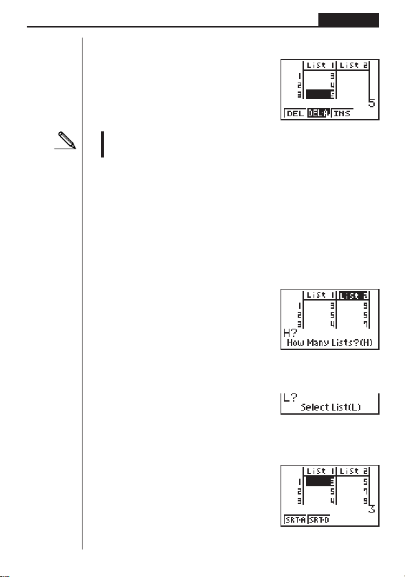
85
List Function Chapter 6
3. Input the value you want into the new cell (4 in our example) and press w.
ew
•Note that the above cell insert operation does not affect cells in other lists. If the
data in the list where you insert a cell is somehow related to the data in
neighboring lists, inserting a cell can cause related values to become misaligned.
kk
kk
k Sorting List Values
You can sort lists into either ascending order or descending order. The current cur-
sor location does not matter in the following procedures.
uu
uu
uTo sort a single list
Ascending order
1. While the lists are on the screen, press [ to display the Operation Menu and
then press 1 (SRT-A).
[1(SRT-A)
2. The prompt “How Many Lists? (H)” appears to ask how many lists you want to
sort. Here we will input 1 to indicate we want to sort only one list.
bw
3. In response to the “Select List (L)” prompt, input the number of the list you want to
sort. Here we will input 2 to specify sorting of List 2.
cw
The values in List 2 are sorted into ascending order.
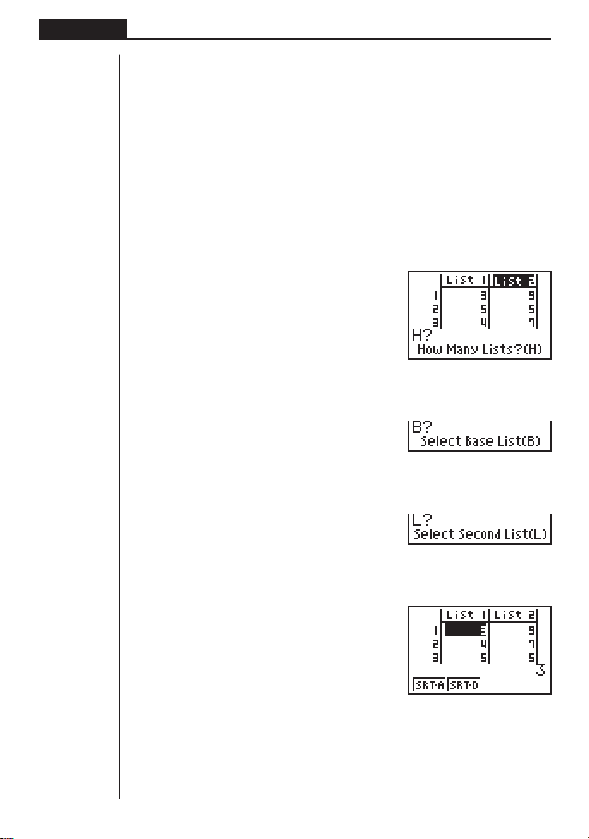
86
Chapter 6 List Function
Descending order
Use the same procedure as that for the ascending order sort. The only difference is
that you should press 2 (SRT-D) in place of 1 (SRT-A).
uu
uu
uTo sort multiple lists
You can link multiple lists together for a sort so that all of their cells are rearranged in
accordance with the sorting of a base list. The base list is sorted into either ascend-
ing order or descending order, while the cells of the linked lists are arranged so that
the relative relationship of all the rows is maintained.
Ascending order
1. While the lists are on the screen, press 1 (SRT-A).
1(SRT-A)
2. The prompt “How Many Lists? (H)” appears to ask how many lists you want to
sort. Here we will sort one base list linked to one other list, so we should input 2.
cw
3. In response to the “Select Base List (B)” prompt, input the number of the list you
want to sort into ascending order. Here we will specify List 1.
bw
4. In response to the “Select Second List (L)” prompt, input the number of the list
you want to link to the base list. Here we will specify List 2.
cw
The values in List 1 are sorted into ascending order, and the cells of List 2 are also
rearranged to keep the same relationship with the List 1 cells.
Descending order
Use the same procedure as that for the ascending order sort. The only difference is
that you should press 2 (SRT-D) in place of 1 (SRT-A).

87
List Function Chapter 6
3. Manipulating List Data
List data can be used in arithmetic and function calculations. There is also a collec-
tion of powerful list data manipulation functions that let you do the following.
•Count the number values (Dim)
•Replace all cell values with the same value (Fill)
•Generate a sequence of numbers (Seq)
•Find the minimum value in a list (Min)
•Find the maximum value in a list (Max)
•Find which of two lists contains the smallest value (Min)
•Find which of two lists contains the greatest value (Max)
•Calculate the mean of list values (Mean)
•Calculate the mean of values of specified frequency (Mean)
•Calculate the median of values in a list (Med)
•Calculate the median of values of specifies frequency (Med)
•Calculate the sum of values in a list (Sum)
You can use list data manipulation functions in the RUN, STAT, LIST, TABLE, or
PRGM Mode.
kk
kk
k Accessing the List Data Manipulation Function Menu
All of the following examples are performed in the RUN Mode.
Press K and then 1 (LIST). This menu has three pages and you can advance to
the next page by pressing [.
Note that all closing parentheses at the end of the following operations can be omitted.
uu
uu
uTo count the number of values (Dim)
K1(LIST)3(Dim)1(List) <list number 1-6> w
• The number of cells that contain data in a list is called its “dimension.”
Example To enter the RUN Mode and count the number of values in List 1
(36, 16, 58, 46, 56)
AK1(LIST)3(Dim)
1(List)bw
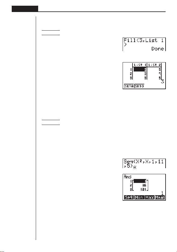
88
Chapter 6 List Function
uu
uu
uTo replace all cell values with the same value (Fill)
K 1 (LIST) 4 (Fill) <value> , 1 (List) <list number 1-6> ) w
Example To replace all values in List 1
(36, 16, 58, 46, 56)
with the number 3
AK1(LIST)4(Fill)
d,1(List)b)w
The following shows the new contents of List 1.
uu
uu
uTo generate a sequence of numbers (Seq)
K 1 (LIST) [1 (Seq) <expression> , <variable name> ,
<start value> , <end value> , <pitch> ) w
• The result of this operation is also stored in Ans Memory.
Example To input the number sequence 1
2
, 6
2
, 11
2
into a list
Use the following settings.
Variable:
x
Starting value: 1
Ending value: 11
Pitch: 5
AK1(LIST)[1(Seq)
Tx,T,b,bb,f)
w
Specifying an ending value of 12, 13, 14, or 15 produces the same result as shown
above, because all of them are less than the value produced by the next increment (16).
The resulting sequence is input into Ans Memory.
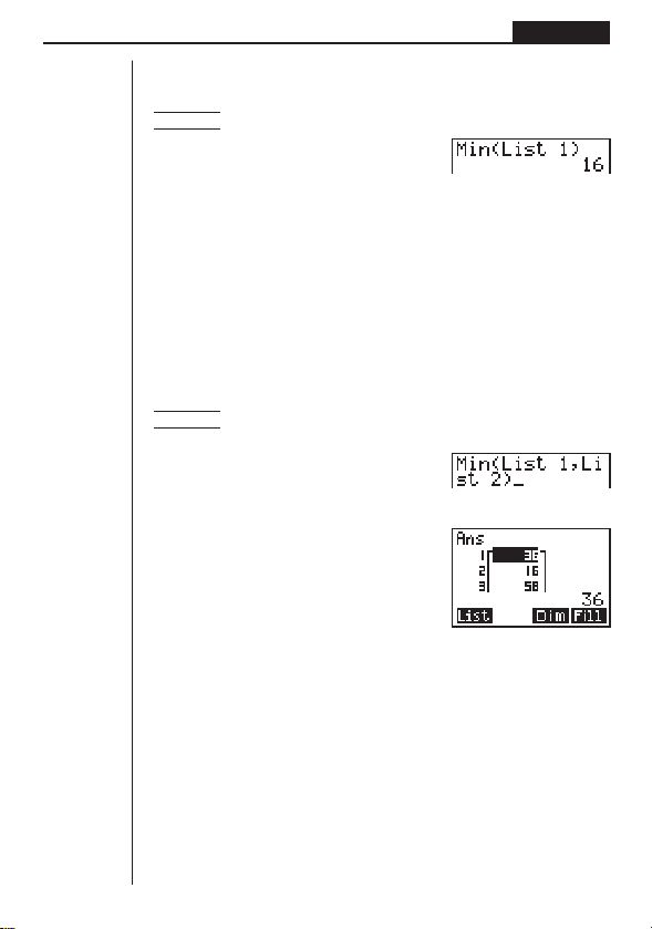
89
List Function Chapter 6
uu
uu
uTo find the minimum value in a list (Min)
K 1 (LIST) [ 2 (Min) [ [ 1 (List) <list number 1-6> ) w
Example To find the minimum value in List 1 (36, 16, 58, 46, 56)
AK1(LIST)[2(Min)
[[1(List)b)w
uu
uu
uTo find the maximum value in a list (Max)
Use the same procedure as when finding the minimum value, except press 3 (Max)
in place of 2 (Min).
uu
uu
uTo find which of two lists contains the smallest value (Min)
K 1 (LIST) [ 2 (Min) [[ 1 (List) <list number 1-6> ,
1 (List) <list number 1-6> ) w
• The two lists must contain the same number of data items. Otherwise, an error
(Dim ERROR) occurs.
• The result of this operation is also stored in Ans Memory.
Example To find whether List 1 (75, 16, 98, 46, 56) or List 2 (36, 89, 58, 72,
67) contains the smallest value
AK1(LIST)[2(Min)
[[1(List)b,
1(List)c)
w
uu
uu
uTo find which of two lists contains the greatest value (Max)
Use the same procedure as that for the smallest value, except press 3 (Max) in
place of 2 (Min).
• The two lists must contain the same number of data items. Otherwise, an error
(Dim ERROR) occurs.
uu
uu
uTo calculate the mean of list values (Mean)
K 1 (LIST) [ 4 (Mean) [ [ 1 (List) <list number 1-6> ) w
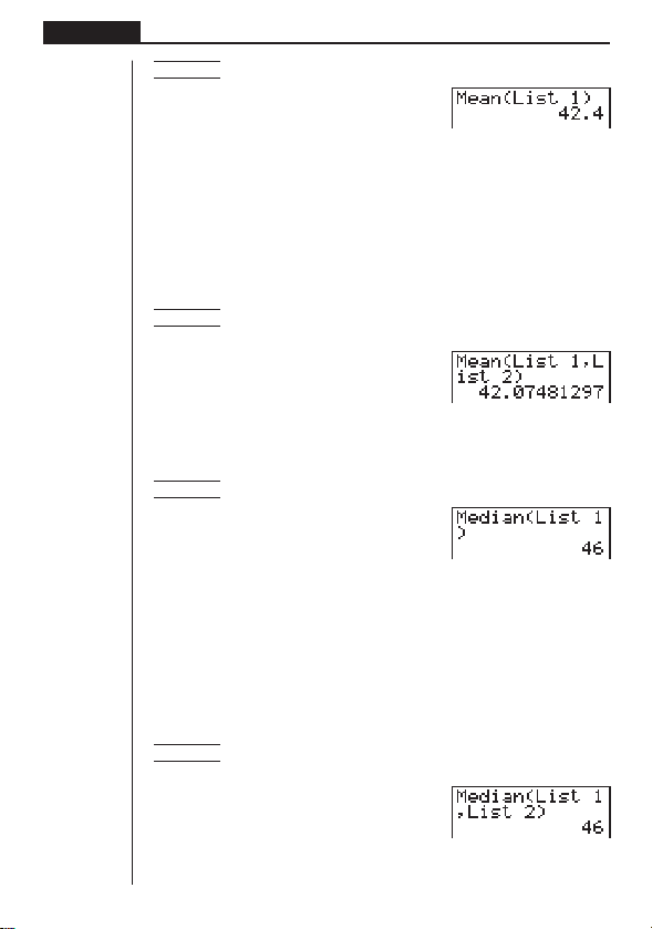
90
Chapter 6 List Function
Example To calculate the mean of values in List 1 (36, 16, 58, 46, 56)
AK1(LIST)[4(Mean)
[[1(List)b)w
uu
uu
uTo calculate the mean of values of specified frequency (Mean)
This procedure uses two lists: one that contains values and one that contains the
number of occurrences of each value. The frequency of the data in Cell 1 of the first
list is indicated by the value in Cell 1 of the second list, etc.
• The two lists must contain the same number of data items. Otherwise, an error
(Dim ERROR) occurs.
K 1 (LIST) [ 4 (Mean) [ [ 1 (List) <list number 1-6(data)>
, 1 (List) <list number 1-6 (frequency)> ) w
Example To calculate the mean of values in List 1 (36, 16, 58, 46, 56), whose
frequency is indicated by List 2 (75, 89, 98, 72, 67)
AK1(LIST)[4(Mean)
[[1(List)b,1(List)c)w
uu
uu
uTo calculate the median of values in a list (Med)
K 1 (LIST) [ [ 1 (Med) [ 1 (List) <list number 1-6> ) w
Example To calculate the median of values in List 1 (36, 16, 58, 46, 56)
AK1(LIST)[[1(Med)
[1(List)b)w
uu
uu
uTo calculate the median of values of specified frequency (Med)
This procedure uses two lists: one that contains values and one that contains the
number of occurrences of each value. The frequency of the data in Cell 1 of the first
list is indicated by the value in Cell 1 of the second list, etc.
• The two lists must contain the same number of data items. Otherwise, an error
(Dim ERROR) occurs.
K 1 (LIST) [ [ 1 (Med) [ 1 (List) <list number 1-6 (data)>
, 1 (List) <list number 1-6 (frequency)> ) w
Example To calculate the median of values in List 1 (36, 16, 58, 46, 56),
whose frequency is indicated by List 2 (75, 89, 98, 72, 67)
AK1(LIST)[[1(Med)
[1(List)b,1(List)c)w
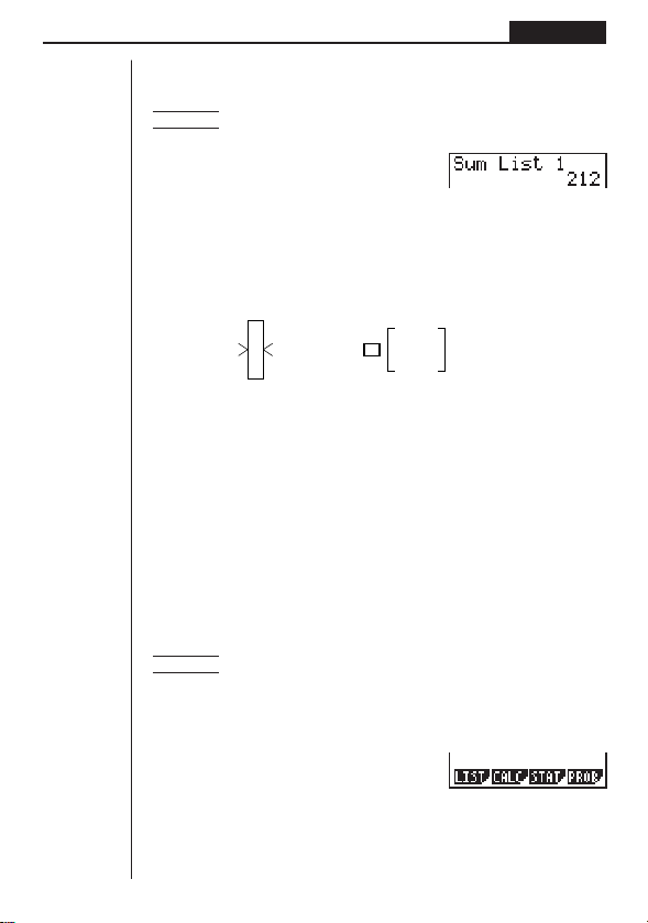
91
List Function Chapter 6
uu
uu
uTo calculate the sum of values in a list (Sum)
K 1 (LIST) [ [ 2 (Sum) [ 1 (List) <list number 1-6> w
Example To calculate the sum of values in List 1 (36, 16, 58, 46, 56)
AK1(LIST)[[2(Sum)
[1(List)bw
4. Arithmetic Calculations Using Lists
You can perform arithmetic calculations using either two lists or one list and a numeric
value.
List
Numeric Value
List
Numeric Value
+
−
×
÷
=
List
Ans Memory
kk
kk
k Error Messages
•A calculation involving two lists performs the operation between corresponding
cells. Because of this, a Dim ERROR occurs if the two lists do not have the same
number of values (which means they have different “dimensions”).
•An Ma ERROR occurs whenever an operation involving any two cells generates
a mathematical error.
kk
kk
k Inputting a List into a Calculation
There are two methods you can use to input a list into a calculation.
uu
uu
uTo input a specific list by name
Example To input List 6
1. Press K to display the first Operation Menu.
• This is the function key menu that appears in the RUN or PRGM Mode when you
press K.
K
Calculation results are
stored in Ans Memory.
1234

92
Chapter 6 List Function
2. Press 1 (LIST) to display the List Data Manipulation Menu.
1(LIST)
3. Press 1 (List) to display the “List” command and input the number of the list you
want to specify.
1(List)g
(Input List 6.)
uu
uu
uTo directly input a list of values
You can also directly input a list of values using {, }, and ,.
41 6
Example To multiply List 3 65 by the list 0
22 4
K1(LIST)1(List)d*!{g,a,e!}w
246
The resulting list
0 is stored in Ans Memory.
88
uu
uu
uTo assign the contents of one list to another list
Use a to assign the contents of one list to another list.
Example 1 To assign the contents of List 3 to List 1
K1(LIST)1(List)da1(List)bw
In place of 1 (List) d in the above procedure, you could input !{eb,
gf,cc!}.
Example 2 To assign the list in Ans Memory to List 1
K1(LIST)1(List)!Ka1(List)bw
uu
uu
uTo input a single list cell value into a calculation
You can extract the value in a specific cell of a list and use it in a calculation. Specify
the cell number by enclosing it between square brackets using the [ and ] keys.
Example To calculate the sine of the value stored in Cell 3 of List 2
sK1(LIST)1(List)c![d!]w
1 234

93
List Function Chapter 6
uu
uu
uTo input a value into a specific cell
You can input a value into a specific cell inside a list. When you do, the value that
was previously stored in the cell is replaced with the new value you input.
Example To input the value 25 into cell 2 of List 3
cfaK1(LIST)1(List)d![c!]w
kk
kk
k Recalling List Contents
Example To recall the contents of List 1
K1(LIST)1(List)bw
• The above operation displays the contents of the list you specify and stores them
in Ans Memory, which allows you to use the Ans Memory contents in a calcula-
tion.
uu
uu
uTo use list contents in Ans Memory in a calculation
Example To multiply the list contents in Ans Memory by 36
K1(LIST)1(List)!K*dgw
• The operation K 1 (LIST) 1 (List) ! K recalls Ans Memory contents.
• This operation replaces current Ans Memory contents with the result of the above
calculation.
kk
kk
k Graphing a Function Using a List
When using the graphing functions of this calculator, you can input a function such
as Y1 = List1 X. If List 1 is {1,2,3}, this function will produces three graphs: Y = X, Y =
2X, Y = 3X.
There are certain limitations on using lists with graphing functions.
kk
kk
k Inputting Scientific Calculations into a List
You can use the numeric table generation functions in the Table Mode to input values
that result from certain scientific function calculations into a list. To do this, first gen-
erate a table. Next, use the “list copy” function to copy the values from the table to the
list.
P. 7 8

94
Chapter 6 List Function
kk
kk
k Performing Scientific Function Calculations Using a List
Lists can be used just as numeric values are in scientific function calculations. When
the calculation produces a list as a result, the list is stored in Ans Memory.
41
Example 1 To use List 3 65 to perform sin (List 3)
22
Use radians as the angle unit
sK1(LIST)1(List)dw
–0.158
The resulting list
0.8268 is stored in Ans Memory.
–8E–3
In place of 1 (List) d in the above procedure, you could input !{eb,g
f,cc!}.
14
Example 2 To use List 1 2 and List 2 5 to perform List 1
List 2
36
K1(LIST)1(List)bM1(List)cw
This creates a list with the results of 1
4
, 2
5
, 3
6
.
1
The resulting list 32 is stored in Ans Memory.
729

Statistical Graphs and
Calculations
This chapter describes how to input statistical data into lists, and
how to calculate the mean, maximum and other statistical values. It
also tells you how to perform regression calculations.
1. Before Performing Statistical Calculations
2. Statistical Calculation Examples
3. Calculating and Graphing Single-Variable Statistical Data
4. Calculating and Graphing Paired-Variable Statistical Data
5. Manual Graphing
6. Performing Statistical Calculations
Chapter
7
Important!
• This chapter contains a number of graph screen shots. In each case, new data
values were input in order to highlight the particular characteristics of the graph
being drawn. Note that when you try to draw a similar graph, the unit uses data
values that you have input using the List function. Because of this, the graphs
that appears on the screen when you perform a graphing operation will prob-
ably differ somewhat from those shown in this manual.
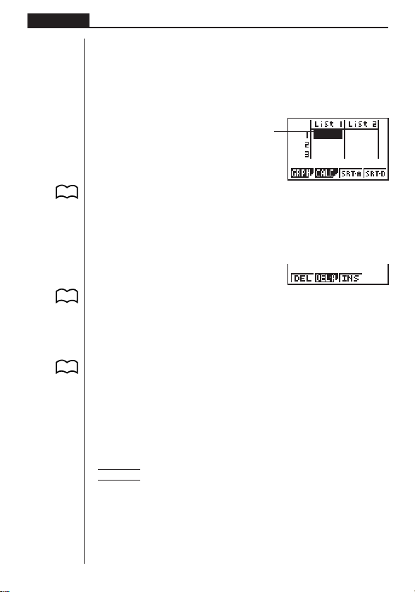
96
Chapter 7 Statistical Graphs and Calculations
1. Before Performing Statistical
Calculations
In the Main Menu, select the STAT icon to enter the STAT Mode and display the
statistical data lists.
Use the statistical data lists to input data and to perform statistical calculations.
1 (GRPH) .... Graph menu
2 (CALC) ..... Statistical calculation menu
3 (SRT•A) .... Ascending sort
4 (SRT•D) .... Descending sort
[
1 (DEL) ........ Single data item delete
2 (DEL•A) .... Delete all data
3 (INS) ......... Insert data item
Press [ to return to the previous menu.
• The procedures you should use for data editing are identical to those you use
with the list function. For details, see “Chapter 6 List Function”.
2. Statistical Calculation Examples
Once you input data, you can use it to produce a graph and check for tendencies.
You can also use a variety of different regression calculations to analyze the data.
Example To input the following two data groups and perform statistical
calculations
0.5, 1.2, 2.4, 4.0, 5.2
–2.1, 0.3, 1.5, 2.0, 2.4
1234[
1234 [
P. 8 3
P. 8 4
P. 8 4
P. 7 9
Use
f
,
c
,
d
and
e
to move
the highlighting around the lists.
P. 9 7
P. 121
P. 8 5
P. 8 6
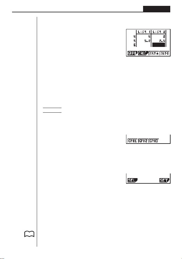
97
Statistical Graphs and Calculations Chapter 7
kk
kk
k Inputting Data into Lists
Input the two groups of data into List 1 and List 2.
a.fwb.cw
c.ewewf.cw
e
-c.bwa.dw
b.fwcwc.ew
Once data is input, you can use it for graphing and statistical calculations.
•Input values can be up to 10 digits long (9-digit mantissa and 2-digit exponent
when using exponential format). Values in statistical data table cells are shown
only up to six digits.
•You can use the f, c, d and e keys to move the highlighting to any cell in
the lists for data input.
kk
kk
k Plotting Data
Example To specify Graph 1 as non-draw (OFF) and Graph 3 as draw (ON)
and use Graph 3 to plot the data you input into statistical data
List 1 and List 2 above
While the statistical data list is on the display, press 1 (GRPH) to display the graph
menu.
1(GRPH)
1 (GPH1) ..... Graph 1 draw
2 (GPH2) ..... Graph 2 draw
3 (GPH3) ..... Graph 3 draw
[
1(SEL) ......... Graph (GPH1, GPH2, GPH3) selection
4(SET) ......... Graph settings (graph type, list assignments)
Press [ to return to the previous menu.
•You can specify the graph draw/non-draw status, the graph type, and other gen-
eral settings for each of the graphs in the graph menu (GPH1, GPH2, GPH3).
•You can press any function key (1,2,3) to draw a graph regardless of the
current location of the highlighting in the statistical data list.
• The initial default graph type setting for all the graphs (Graph 1 through Graph 3)
is scatter diagram, but you can change to one of a number of other graph types.
P. 9 9
1234 [
1 234 [
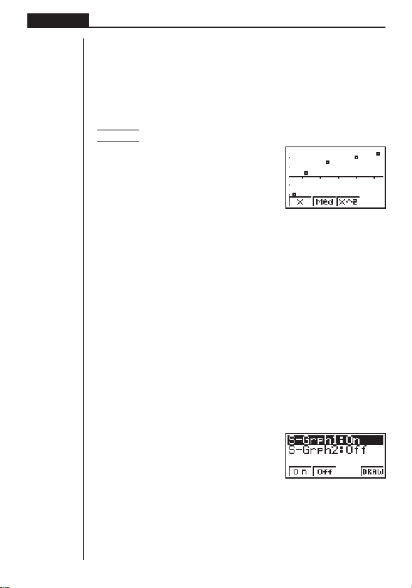
98
Chapter 7 Statistical Graphs and Calculations
kk
kk
k Plotting a Scatter Diagram
It is often difficult to spot the relationship between two sets of data (such as height
and shoe size) by simply looking at the numbers. Such relationships often become
clear however, when we plot the data on a graph, using one set as
x-values and the
other set as
y-values.
uu
uu
uTo plot a scatter diagram
Example To plot the data we input in statistical data List 1 and List 2
1(GPH1)
• The default setting automatically uses List 1 data as x-axis values and List 2 data
as
y-axis values. Each set of x/y data is a point on the scatter diagram.
•To return to the statistical data list, press Q.
kk
kk
k Changing Graph Parameters
Use the following procedures to specify the graph draw/non-draw status, the graph
type, and other general settings for each of the graphs in the graph menu (GPH1,
GPH2, GPH3).
1. Graph draw/non-draw status (SELECT)
The following procedure can be used to specify the draw (On)/non-draw (Off) status
of each of the graphs in the graph menu.
uu
uu
uTo specify the draw/non-draw status of a graph
1. While the graph menu is on the display, press [1 (SEL) to display the graph
On/Off screen.
1(GRPH)
[1(SEL)
1 (On) .......... Graph On (graph draw)
2 (Off) .......... Graph Off (graph non-draw)
4 (DRAW) .... Draw all On graphs
•Note that the S-Grph1 setting is for Graph 1 (GPH1 of the graph menu), S-Grph2
is for Graph 2, and S-Grph3 is for Graph 3.
123 4

99
Statistical Graphs and Calculations Chapter 7
2. Use f and c to move the highlighting to the graph whose draw (On)/non-draw
(Off) status you want to change and press 1 (On) or 2 (Off).
3. To return to the graph menu, press Q.
uu
uu
uTo draw a graph
Example To draw a scatter diagram of Graph 3 only
1(GRPH)[1(SEL)
2(Off)
cc1(On)
4(DRAW)
2. General graph settings (SET)
This section describes how to use the general graph settings screen to make the
following settings for each graph (GPH1, GPH2, GPH3).
• Graph Type
The initial default graph type setting for all the graphs is scatter graph. You can select
one of a variety of other statistical graph types for each graph.
• List or Data
The initial default statistical data is List 1 for single-variable data, and List 1 and List
2 for paired-variable data. You can specify which statistical data list you want to use
to draw the graph.
• Frequency
Normally, each data item or data pair in the statistical data list is represented on a
graph as a point. When you are working with a large number of data items however,
this can cause problems because of the number of plot points on the graph. When
this happens, you can specify a frequency list that contains values indicating the
number of instances (the frequency) of the data items in the corresponding cells of
the lists you are using for
x-data and y-data. Once you do this, only one point is
plotted for the multiple data items, which makes the graph easier to read.
• Mark Type
This setting lets you specify the shape of the plot points on the graph.
123 4
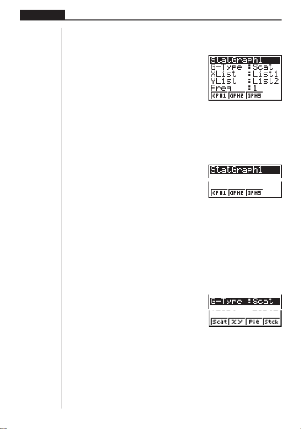
100
Chapter 7 Statistical Graphs and Calculations
1234
1234[
uu
uu
uTo display the general graph settings (SET) screen
While the graph menu is on the display, press [4 (SET) to display the general
graph settings screen.
1(GRPH)
[4(SET)
• The settings shown here are examples only. The settings on your general graph
settings screen may differ.
uu
uu
uTo select the StatGraph area
1. While the general graph settings screen is on the display, use f and c to
move the highlighting to the StatGraph item.
2. Use the function key menu to select the StatGraph area you want to select.
1 (GPH1) ..... Graph 1
2 (GPH2) ..... Graph 2
3 (GPH3) ..... Graph 3
uu
uu
uTo select the graph type (G-Type)
1. While the general graph settings screen is on the display, use f and c to
move the highlighting to the G-Type item.
2. Use the function key menu to select the graph type you want to select.
1 (Scat) ........ Scatter diagram
2 (
xy) ........... xy line graph
3 (Pie) .......... Pie chart
4 (Stck) ........ Stacked bar chart
101
Statistical Graphs and Calculations Chapter 7
1234 [
1234 [
1234 [
1234 [
1234[
[
1 (Hist) ......... Histogram
2 (Box) ......... Med-box graph
3 (N•Dis) ...... Normal distribution curve
[
1 (X) ............ Linear regression graph
2 (Med) ........ Med-Med graph
3 (X^2) ......... Quadratic regression graph
[
1 (Log) ......... Logarithmic regression graph
2 (Exp) ......... Exponential regression graph
3 (Pwr) ......... Power regression graph
[
1 (Bar) ......... Bar graph
2 (Line) ........ Line graph
3 (Both) ....... Bar graph and line graph
Press [ to return to the previous menu.
uu
uu
uTo select the
x-axis data list (XList)
1. While the graph settings screen is on the display, use f and c to move the
highlighting to the XList item.

102
Chapter 7 Statistical Graphs and Calculations
2. Use the function key menu to select the name of the statistical data list whose
values you want on the
x-axis of the graph.
1 (List1) ....... List 1
2 (List2) ....... List 2
3 (List3) ....... List 3
4 (List4) ....... List 4
[
1 (List5) ....... List 5
2 (List6) ....... List 6
Press [ to return to the previous menu.
uu
uu
uTo select the
y-axis data list (YList)
1. While the graph settings screen is on the display, use f and c to move the
highlighting to the YList item.
2. Use the function key menu to select the name of the statistical data list whose
values you want on the
y-axis of the graph.
1 (List1) ....... List 1
2 (List2) ....... List 2
3 (List3) ....... List 3
4 (List4) ....... List 4
[
1 (List5) ....... List 5
2 (List6) ....... List 6
Press [ to return to the previous menu.
1234[
1234[
1234[
103
Statistical Graphs and Calculations Chapter 7
uu
uu
uTo select the frequency data list (Freq)
1. While the general graph settings screen is on the display, use f and c to
move the highlighting to the Freq item.
2. Use the function key menu to select the frequency setting you want.
1 (1) ............. Plot all data (1-to-1)
2 (List1) ....... List 1 data is frequency data.
3 (List2) ....... List 2 data is frequency data.
4 (List3) ....... List 3 data is frequency data.
[
1 (List4) ....... List 4 data is frequency data.
2 (List5) ....... List 5 data is frequency data.
3 (List6) ....... List 6 data is frequency data.
Press [ to return to the previous menu.
uu
uu
uTo select the plot mark type (M-Type)
1. While the general graph settings screen is on the display, use f and c to
move the highlighting to the M-Type item.
2. Use the function key menu to select the plot mark you want to select.
1 (
) ............ Plot using
2 (X) ............ Plot using X
3 (•).............. Plot using •
1234
1234 [
1234[
104
Chapter 7 Statistical Graphs and Calculations
1234[
1234[
1234[
1234[
uu
uu
uTo select the data list for a pie chart, stacked bar chart, bar graph
or line graph (Data)
1. While the graph settings screen is on the display, use f and c to move the
highlighting to the Data item.
2. Use the function key menu to select the name of the statistical data list whose
values you want to use.
1 (List1) ....... List 1
2 (List2) ....... List 2
3 (List3) ....... List 3
4 (List4) ....... List 4
[
1 (List5) ....... List 5
2 (List6) ....... List 6
Press [ to return to the previous menu.
uu
uu
uTo select the data list for a combined bar graph and line graph (Both)
1. While the graph settings screen is on the display, use f and c to move the
highlighting to the Bar item.
2. Use the function key menu to select the name of the statistical data list whose
values you want to use.
1 (List1) ....... List 1
2 (List2) ....... List 2
3 (List3) ....... List 3
4 (List4) ....... List 4
[
1 (List5) ....... List 5
2 (List6) ....... List 6
Press [ to return to the previous menu.

105
Statistical Graphs and Calculations Chapter 7
3. Use f and c to move the highlighting to the Line item.
4. Use the function key menu to select the name of the statistical data list whose
values you want to use.
1 (List1) ....... List 1
2 (List2) ....... List 2
3 (List3) ....... List 3
4 (List4) ....... List 4
[
1 (List5) ....... List 5
2 (List6) ....... List 6
Press [ to return to the previous menu.
kk
kk
k Drawing an xy Line Graph
Paired data items can be used to plot a scatter diagram. A scatter diagram where the
points are linked is an
xy line graph.
Press Q to return to the statistical data list.
kk
kk
k Selecting the Regression Type
After you graph statistical data, you can use the function menu at the bottom of the
display to select from a variety of different types of regression.
1 (X) ............ Linear regression
2 (Med) ........ Med-Med line
3 (X^2) ......... Quadratic regression
P. 100
(G-Type)
(
xy)
1234[
1234 [
1234[
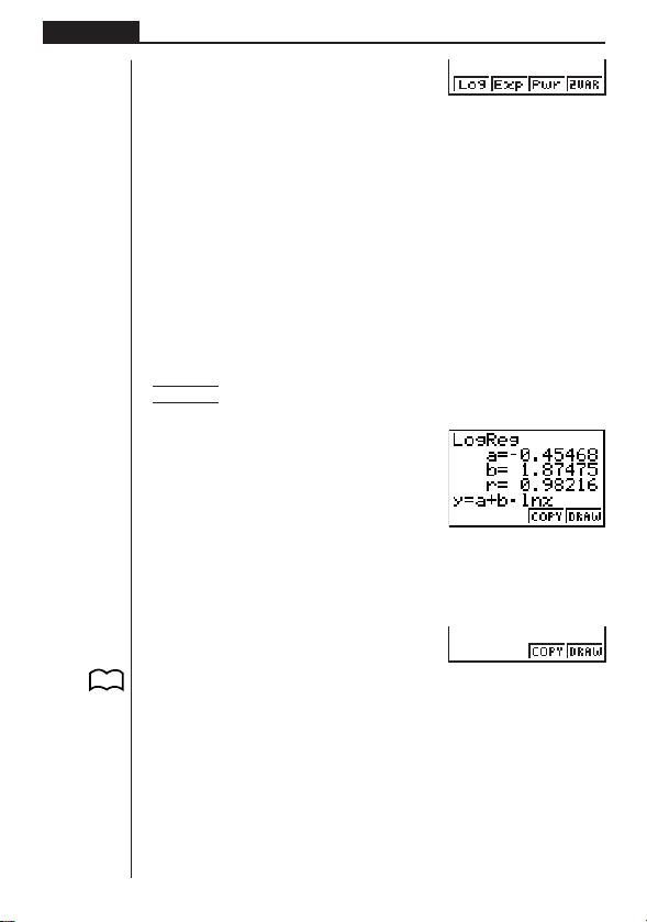
106
Chapter 7 Statistical Graphs and Calculations
[
1 (Log) ......... Logarithmic regression
2 (Exp) ......... Exponential regression
3 (Pwr) ......... Power regression
4 (2VAR) ...... Paired-variable statistical results
Press [ to return to the previous menu.
kk
kk
k Displaying Statistical Calculation Results
Whenever you perform a regression calculation, the regression formula parameter
(such as
a and b in the linear regression y = ax + b) calculation results appear on the
display. You can use these to obtain statistical calculation results.
Regression parameters are calculated as soon as you press a function key to select
a regression type while a graph is on the display.
Example To display logarithmic regression parameter calculation results
while a scatter diagram is on the display
[1(Log)
kk
kk
k Graphing statistical calculation results
You can use the parameter calculation result menu to graph the displayed regres-
sion formula.
3 (COPY)..... Stores the displayed regression formula as a graph function
4 (DRAW) .... Graphs the displayed regression formula
P. 1 1 9
1234
1234
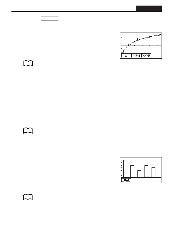
107
Statistical Graphs and Calculations Chapter 7
Example To graph a logarithmic regression
While logarithmic regression parameter calculation results are on the display, press
4 (DRAW).
4(DRAW)
For details on the meanings of function menu items at the bottom of the display, see
“Selecting the Regression Type”.
3. Calculating and Graphing Single-
Variable Statistical Data
Single-variable data is data with only a single variable. If you are calculating the
average height of the members of a class for example, there is only one variable
(height).
Single-variable statistics include distribution and sum. The following three types of
graphs are available for single-variable statistics.
kk
kk
k Histogram
From the statistical data list, press 1 (GRPH) to display the graph menu, press
[4 (SET), and then change the graph type of the graph you want to use (GPH1,
GPH2, GPH3) to histogram.
Input data into a list, make the required settings, and then draw the graph.
kk
kk
k Box Graph
This type of graph lets you see how a large number of data items are grouped within
specific ranges. A box encloses all the data in an area from the first quartile (Q1) to
the third quartile (Q3), with a line drawn at the median (Med). Lines (called whiskers)
extend from either end of the box up to the minimum and maximum of the data.
From the statistical data list, press 1 (GRPH) to display the graph menu, press
[4 (SET), and then change the graph type of the graph you want to use (GPH1,
GPH2, GPH3) to box graph.
P. 105
P. 101
(G-Type)
(Hist)
P. 101
(G-Type)
(Box)
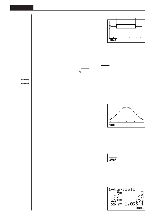
108
Chapter 7 Statistical Graphs and Calculations
P. 101
(G-Type)
(N•Dis)
Med
Q3
1 234
Q1
maxX
kk
kk
k Normal Distribution Curve
The normal distribution curve is graphed using the following normal distribution func-
tion.
y
=
1
(2 π) xσ
n
e
–
2x σ
n
2
(
x –
x
)
2
The distribution of characteristics of items manufactured according to some fixed
standard (such as component length) fall within normal distribution. The more data
items there are, the closer the distribution is to normal distribution.
From the statistical data list, press 1 (GRPH) to display the graph menu, press
[4 (SET), and then change the graph type of the graph you want to use (GPH1,
GPH2, GPH3) to normal distribution.
kk
kk
k Displaying Single-Variable Statistical Results
Single-variable statistics can be expressed as both graphs and parameter values.
When these graphs are displayed, the menu at the bottom of the screen appears as
below.
1 (1VAR) ...... Single-variable calculation result menu
Pressing 1 (1VAR) displays the following screen.
1(1VAR)
minX
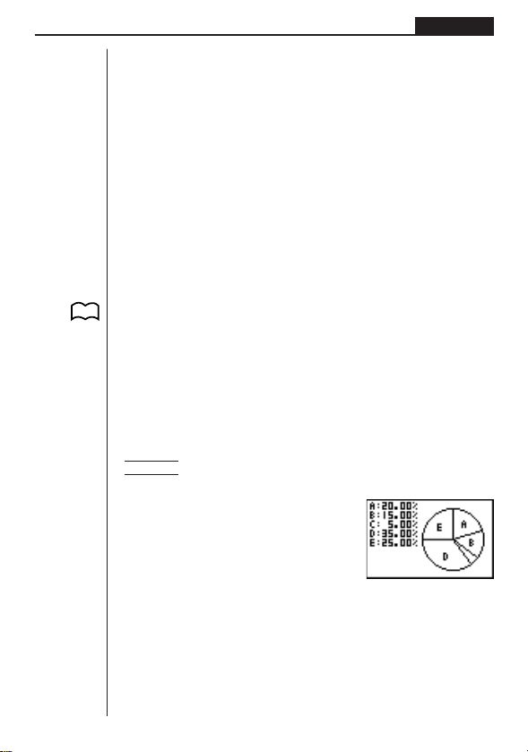
109
Statistical Graphs and Calculations Chapter 7
The following describes the meaning of each of the parameters.
_
x ...................... Mean of data
Σ
x .................... Sum of data
Σ
x
2
.................. Sum of squares
xσn .................. Population standard deviation
xσn-1 ................ Sample standard deviation
n ...................... Number of data items
minX................ Minimum
Q1 ................... First quartile
Med ................. Median
Q3 ................... Third quartile
maxX............... Maximum
Mod ................. Mode
•Press 4 (DRAW) to return to the original single-variable statistical graph.
kk
kk
k Pie Chart
From the statistical data list, press 1 (GRPH) to display the graph menu, press [
4 (SET), and then change the graph type of the graph you want to use (GPH1,
GPH2, GPH3) to pie chart. Next, move the highlighting to “Display” and then press
1 or 2 to select the pie chart data format.
1 (%) ............ Displayed values show what percentage of the total data each
pie segment represents.
2 (Data) ....... Displayed values show actual data.
Press Q to draw the chart.
Example To input the following data into List 1 and use it to draw a pie
chart: 18.0, 13.5, 4.5, 31.5, 22.5
1(GRPH)[4(SET)
1(GPH1)c
3(Pie)c
1(List1)c
1(%)Q
1(GRPH)1(GPH1)
•A pie chart can have up to eight data items. Attempting to draw a pie chart for a
list that has more than eight data items causes an error (Dim ERROR).
•Only positive data can be included in a pie chart. Attempting to draw a pie chart
for a list that includes negative data causes an error (Ma ERROR).
•View Window settings are not applied to pie charts.
•A pie chart cannot be superimposed with another graph.
•Values appearing on a pie chart are automatically assigned to the corresponding
variables (A, B, C, etc.)
P. 100
(G-Type)
(Pie)
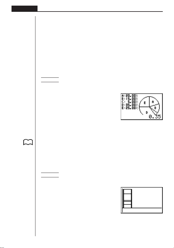
110
Chapter 7 Statistical Graphs and Calculations
•Performing a trace operation (!1 (TRCE)) while a pie chart is on the display
causes the pointer to appear at the topmost segment. Pressing e and d moves
the pointer to neighboring segments.
•While a pie graph is on the display, you can toggle between the two data formats
(percent and data) by pressing !4 (CHNG).
•You cannot draw multiple pie charts on the same screen.
•Percent values shown on pie charts are cut off to two decimal places.
uu
uu
u Performing Mathematical Operations Using Pie Chart Data
Pressing !3 (GSLV) causes the cursor to appear at the bottom of the screen.
You can then perform mathematical operations using the chart’s data.
Example To perform the operation A + B
After drawing the pie chart, perform the following operation.
!3(GSLV)
aA+aB
w
The result shows that A and B account for 35% of the data.
kk
kk
k Stacked Bar Chart
From the statistical data list, press 1 (GRPH) to display the graph menu, press [
4 (SET), and then change the graph type of the graph you want to use (GPH1,
GPH2, GPH3) to stacked bar chart.
Press Q to draw the chart.
Example To input the following data into List 1 and use it to draw a stacked
bar chart: 18.0, 13.5, 4.5, 31.5, 22.5
1(GRPH)[4(SET)
1(GPH1)c
4(Stck)c
1(List1)Q
1(GRPH)1(GPH1)
•A stacked bar chart can have up to eight data items. Attempting to draw a stacked
bar chart for a list that has more than eight data items causes an error (Dim
ERROR).
P. 100
(G-Type)
(Stck)

111
Statistical Graphs and Calculations Chapter 7
•Only positive data can be included in a stacked bar chart. Attempting to draw a
stacked bar chart for a list that includes negative data causes an error (Ma ER-
ROR).
•A stacked bar chart cannot be superimposed with another graph.
•View Window settings are not applied to stacked bar charts.
• The following display shows what happens if you perform a trace operation (!
1 (TRCE)) while a stacked bar chart is on the display.
•Pressing f and c moves the highlighting up and down within the same graph.
• If you have multiple stacked bar charts on the screen, use d and e to move
between them.
uu
uu
u Linking the Segments of Stacked Bar Charts with Connecting Lines
While multiple stacked bar charts are on the display, press !4(CNCT) to link
their segments with connecting lines.
Redraw the stacked bar charts to clear the connecting lines.
kk
kk
k Bar Graph
From the statistical data list, press 1 (GRPH) to display the graph menu, press [
4 (SET), and then change the graph type of the graph you want to use (GPH1,
GPH2, GPH3) to bar graph.
Press Q to draw the graph.
P. 101
(G-Type)
(Bar)
!1(TRCE)
R
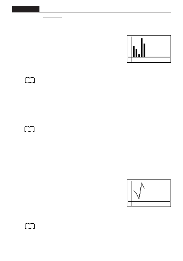
112
Chapter 7 Statistical Graphs and Calculations
Example To input the following data into List 1 and use it to draw a bar
graph: 18.0, 13.5, 4.5, 31.5, 22.5
1(GRPH)[4(SET)
1(GPH1)c
[[[[1(Bar)c
1(List1)Q
1(GRPH)1(GPH1)
•A bar graph can have up to 14 data items. Attempting to draw a bar graph for a
list that has more than 14 data items causes an error (Dim ERROR).
• The
x-axis of a bar graph is fixed. The y-axis is controlled by View Window set-
tings only when Man (manual) is specified for the S-Wind (Statistical Graph View
Window Setting) on the Set Up screen.
•A bar graph can be superimposed with a line graph only. This is done by selecting
3 (Both) while specifying the graph type.
•Pressing ! 1 (TRCE) while a bar graph is on the display activates the trace
operation. Use d and e to move the pointer.
•You cannot draw multiple bar graphs on the same screen.
kk
kk
k Line Graph
From the statistical data list, press 1 (GRPH) to display the graph menu, press [
4 (SET), and then change the graph type of the graph you want to use (GPH1,
GPH2, GPH3) to line graph.
Press Q to draw the graph.
Example To input the following data into List 1 and use it to draw a line
graph: 18.0, 13.5, 4.5, 31.5, 22.5
1(GRPH)[4(SET)
1(GPH1)c
[[[[2(Line)c
1(List1)Q
1(GRPH)1(GPH1)
•A line graph can have up to 14 data items. Attempting to draw a line graph for a
list that has more than 14 data items causes an error (Dim ERROR).
• The
x-axis of a line graph is fixed. The y-axis is controlled by View Window set-
tings only when Man (manual) is specified for the S-Wind (Statistical Graph View
Window Setting) on the Set Up screen.
•A line graph can be superimposed with a bar graph only. This is done by selecting
3 (Both) while specifying the graph type.
P. 8
P. 8
P. 101
(G-Type)
(Line)
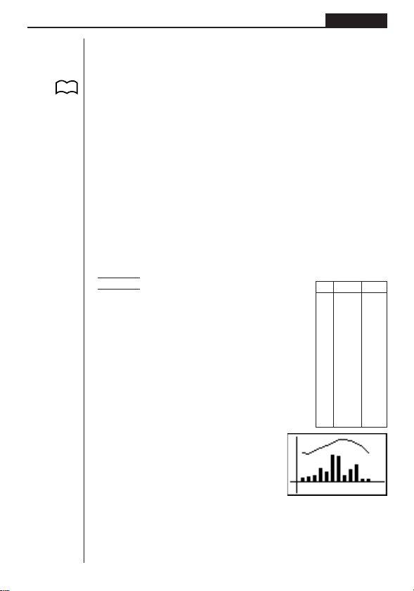
113
Statistical Graphs and Calculations Chapter 7
•Pressing ! 1 (TRCE) while a line graph is on the display activates the trace
operation. Use d and e to move the pointer.
•You cannot draw multiple line graphs on the same screen.
kk
kk
k Bar Graph and Line Graph
From the statistical data list, press 1 (GRPH) to display the graph menu, press
[4 (SET), and then change the graph type of the graph you want to use (GPH1,
GPH2, GPH3) to Both.
When Auto is specified for the S-Wind (Statistical Graph View Window Setting) item
on the Set Up screen, you can next move the highlighting to the AutoWin item and
press 1, 2, or 3 to make one of the following settings.
1 (Sep.G)..... This setting causes each graph to be drawn in different areas
of the display, without superimposing them. The two graphs
share the same
x-coordinates, however, and the x-axis is dis-
played for the bar graph only.
2 (O.Lap) ..... This setting superimposes the two graphs on each other. Each
graph, however, can have its own independent
y-axis values.
3 (Norm) ...... This setting also superimposes the two graphs, with both us-
ing the same
x- and y-coordinates.
Press Q to draw the graph.
Example Draw a graph that shows precipitation in
a certain city as a bar graph and average
temperature as a line graph.
Input the precipitation data into List 1 and
the temperature data into List 2. Use the
following procedure to draw the graph.
1(GRPH)[4(SET)
1(GPH1)c
[[[[3(Both)c
1(List1)c
2(List2)c
1(Sep.G)Q
1(GRPH)1(GPH1)
•Pressing ! 1 (TRCE) while the graph is on the display activates the trace
operation. Use d and e to move the pointer.
•You cannot draw multiple bar and line graphs on the same screen.
List 1 List 2
1 100 5
2 150 4
3 200 11
4 400 16
5 300 20
6 800 24
7 750 31
8 200 32
9 350 29
10 500 24
11 80 18
12 80 6
P. 101
(G-Type)
(Both)
P.8
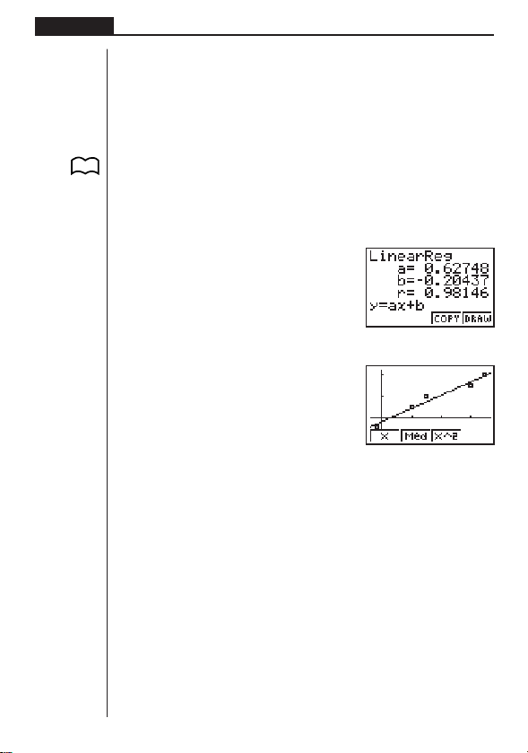
114
Chapter 7 Statistical Graphs and Calculations
4. Calculating and Graphing Paired-
Variable Statistical Data
Under “Plotting a Scatter Diagram,” we displayed a scatter diagram and then per-
formed a logarithmic regression calculation. Let’s use the same procedure to look at
the six regression functions.
kk
kk
k Linear Regression Graph
Linear regression plots a straight line that passes close to as many data points as
possible, and returns values for the slope and
y-intercept (y-coordinate when x = 0)
of the line.
The graphic representation of this relationship is a linear regression graph.
Q1(GRPH)[4(SET)c
1(Scat)
Q1(GRPH)1(GPH1)
1(X)
4(DRAW)
The following are the meanings of the above parameters.
a ...... Regression coefficient (slope)
b ...... Regression constant term (y-intercept)
r ...... Correlation coefficient
(G-Type)
(Scat)
(GPH1)
(X)
P. 105
1234
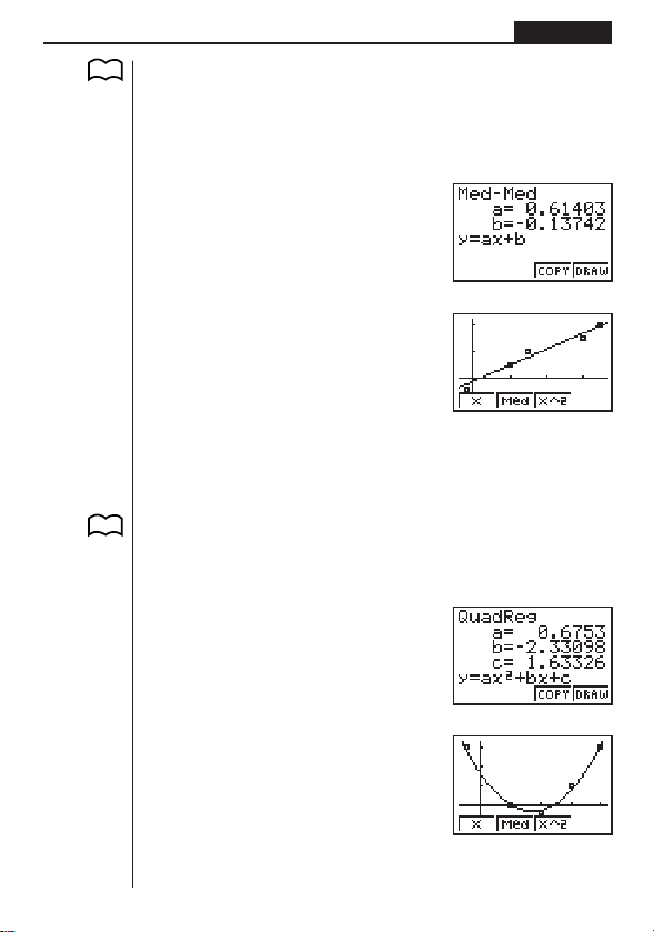
115
Statistical Graphs and Calculations Chapter 7
kk
kk
k Med-Med Graph
When it is suspected that there are a number of extreme values, a Med-Med graph
can be used in place of the least squares method. This is also a type of linear regres-
sion, but it minimizes the effects of extreme values. It is especially useful in produc-
ing highly reliable linear regression from data that includes irregular fluctuations,
such as seasonal surveys.
2(Med)
4(DRAW)
The following are the meanings of the above parameters.
a ...... Med-Med graph slope
b ...... Med-Med graph y-intercept
kk
kk
k Quadratic Regression Graph
A quadratic regression graph represents connection of the data points of a scatter
diagram. It actually is a scattering of so many points that are close enough together
to be connected. The formula that represents this is quadratic regression.
3(X^2)
4(DRAW)
P. 105
1234
1234
P. 105

116
Chapter 7 Statistical Graphs and Calculations
The following are the meanings of the above parameters.
a ...... Regression second coefficient
b ...... Regression first coefficient
c ...... Regression constant term (y-intercept)
kk
kk
k Logarithmic Regression Graph
Logarithmic regression expresses y as a logarithmic function of x. The standard
logarithmic regression formula is
y = a + b × logx, so if we say that X = logx, the
formula corresponds to linear regression formula
y = a + bX.
[1(Log)
4(DRAW)
The following are the meanings of the above parameters.
a ...... Regression constant term
b ...... Regression coefficient (slope)
r ...... Correlation coefficient
kk
kk
k Exponential Regression Graph
Exponential regression expresses y as a proportion of the exponential function of x.
The standard exponential regression formula is
y = a × e
bx
, so if we take the loga-
rithms of both sides we get log
y = loga + bx. Next, if we say Y = logy, and A = loga,
the formula corresponds to linear regression formula Y = A +
bx.
[2(Exp)
P. 106
1234
1234
P. 106
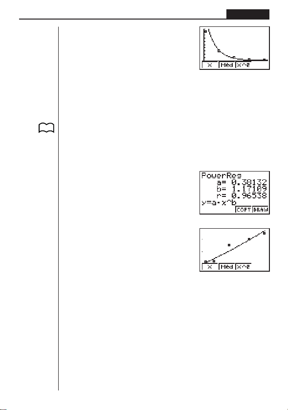
117
Statistical Graphs and Calculations Chapter 7
4(DRAW)
The following are the meanings of the above parameters.
a ...... Regression coefficient
b ...... Regression constant term
r ...... Correlation coefficient
kk
kk
k Power Regression Graph
Exponential regression expresses y as a proportion of the power of x. The standard
power regression formula is
y = a × x
b
, so if we take the logarithms of both sides we
get log
y = loga + b × logx. Next, if we say X = log x, Y = logy, and A = loga, the
formula corresponds to linear regression formula Y = A +
bX.
[3(Pwr)
4(DRAW)
The following are the meanings of the above parameters.
a ...... Regression coefficient
b ...... Regression power
r ...... Correlation coefficient
P. 106
1234
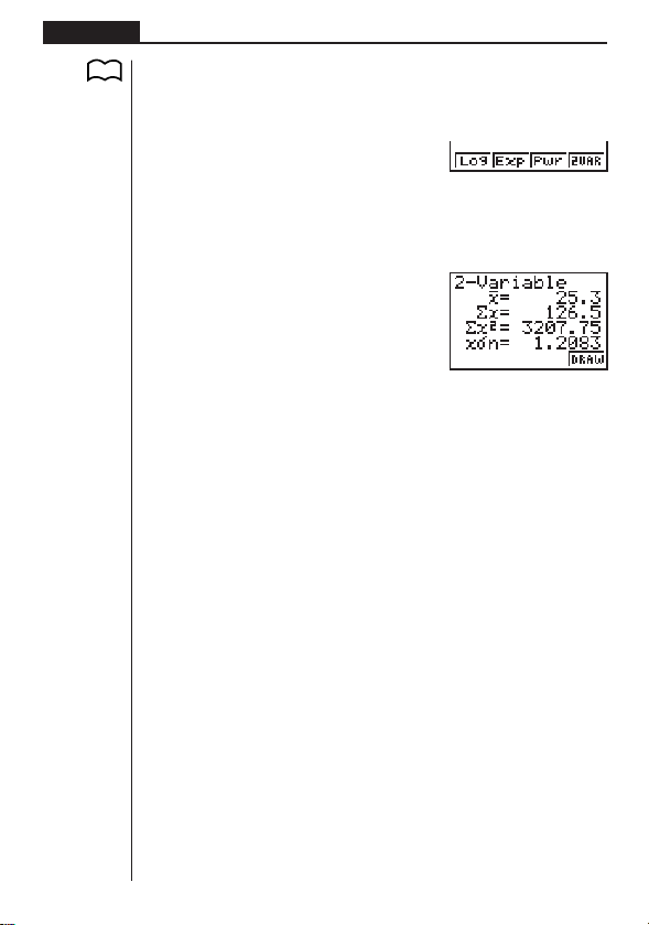
118
Chapter 7 Statistical Graphs and Calculations
kk
kk
k Displaying Paired-Variable Statistical Results
Paired-variable statistics can be expressed as both graphs and parameter values.
When these graphs are displayed, the menu at the bottom of the screen appears as
below.
[
4(2VAR) ....... Paired-variable calculation result menu
Pressing 4 (2VAR) displays the following screen.
4(2VAR)
•Use c to scroll the list so you can view the items that run off the bottom of the
screen. The following describes the meaning of each of the parameters.
_
x ...................... Mean of xList data
Σ
x .................... Sum of xList data
Σ
x
2
.................. Sum of squares of xList data
xσn .................. Population standard deviation of xList data
xσn-1 ................ Sample standard deviation of xList data
n ...................... Number of xList data items
_
y ...................... Mean of yList data
Σ
y .................... Sum of yList data
Σ
y
2
.................. Sum of squares of yList data
yσn .................. Population standard deviation of yList data
yσn-1 ................ Sample standard deviation of yList data
Σ
xy .................. Sum of the product of data stored in xList and yList
minX................ Minimum of
xList data
maxX............... Maximum of
xList data
minY................ Minimum of
yList data
maxY............... Maximum of
yList data
kk
kk
k Copying a Regression Graph Formula to the Graph Mode
After you perform a regression calculation, you can copy its formula to the GRAPH
Mode.
The following are the functions that are available in the function menu at the bottom
of the display while regression calculation results are on the screen.
P. 106
1234
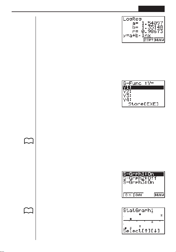
119
Statistical Graphs and Calculations Chapter 7
3 (COPY)..... Stores the displayed regression formula to the GRAPH Mode
4 (DRAW) .... Graphs the displayed regression formula
1. Press 3 (COPY) to copy the regression formula that produced the displayed
data to the GRAPH Mode.
3(COPY)
Note that you cannot edit regression formulas for graph formulas in the GRAPH
Mode.
2. Press w to save the copied graph formula and return to the previous regression
calculation result display.
kk
kk
k Multiple Graphs
You can draw more than one graph on the same display by using the procedure
under “Changing Graph Parameters” to set the graph draw (On)/non-draw (Off) sta-
tus of two or all three of the graphs to draw (On), and then pressing 4 (DRAW).
After drawing the graphs, you can select which graph formula to use when perform-
ing single-variable statistic or regression calculations.
4(DRAW)
1(X)
P. 9 8
1234
P. 105
1234
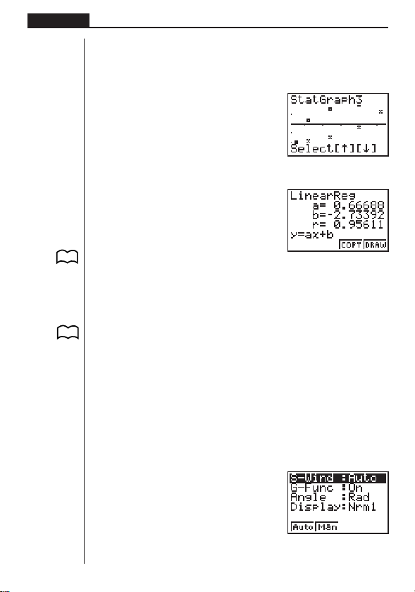
120
Chapter 7 Statistical Graphs and Calculations
• The text at the top of the screen indicates the currently selected graph (StatGraph
1 = Graph 1, StatGraph 2 = Graph 2, StatGraph 3 = Graph 3).
1. Use f and c to change the currently selected graph. The graph name at the
top of the screen changes when you do.
c
2. When graph you want to use is selected, press w.
Now you can use the procedures under “Displaying Single-Variable Statistical Re-
sults” and “Displaying Paired-Variable Statistical Results” to perform statistical cal-
culations.
5. Manual Graphing
In all of the graphing examples up to this point, values were calculated in accord-
ance with View Window settings and graphing was performed automatically. This
automatic graphing is performed when the S-Wind item of the View Window is set to
“Auto” (auto graphing). You can also produce graphs manually, when the automatic
graphing capabilities of this calculator cannot produce the results you want.
kk
kk
k Setting the Width of a Histogram
When the S-Wind item of the View Window is set to “Man” (manual graphing), a
screen appears so you can specify the starting point and spacing of histogram bars.
While the statistical data list is on the display, perform the following procedure.
!Z
P. 108
P. 11 8
P. 8
1 2 34
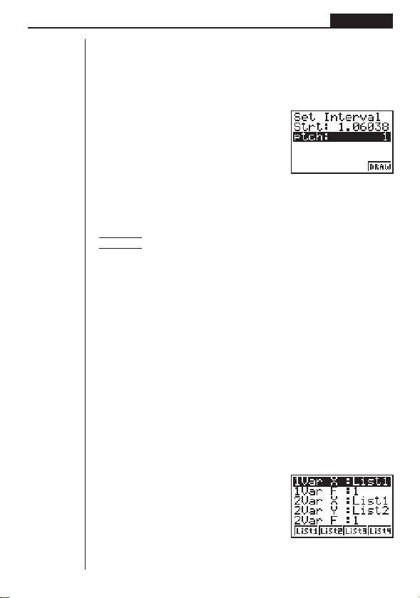
121
Statistical Graphs and Calculations Chapter 7
2(Man)
Q(Returns to previous menu.)
1(GRPH)1(GPH1)
Here we will illustrate this operation by making histogram settings for Graph 1.
The following are the meanings of the items that appear in this screen.
Strt .................. Histogram start point (
x-coordinate)
ptch ................. Bar spacing (specify as scale unit)
Example Strt: 0, ptch: 10
While the statistical data list is on the display, perform the following procedure.
!Z2(Man)
Q(Returns to previous menu.)
1(GRPH)1(GPH1)
aw(Start value is
x = 0.)
baw(pitch = 10)
6. Performing Statistical Calculations
All of the statistical calculations up to this point were performed after displaying a
graph. The following procedures can be used to perform statistical calculations alone.
uu
uu
uTo specify statistical calculation data lists
You have to input the statistical data for the calculation you want to perform and
specify where it is located before you start a calculation. While the statistical data is
on the display, perform the following procedure.
2(CALC)4(SET)
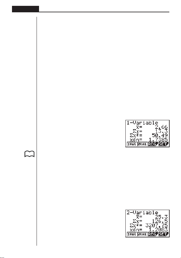
122
Chapter 7 Statistical Graphs and Calculations
The following is the meaning for each item.
1VarX .............. Specifies list where single-variable statistic
x values (XList)
are located.
1VarF .............. Specifies list where single-variable frequency values (Fre-
quency) are located.
2VarX .............. Specifies list where paired-variable statistic
x values (XList)
are located.
2VarY .............. Specifies list where paired-variable statistic
y values (YList)
are located.
2VarF .............. Specifies list where paired-variable frequency values (Fre-
quency) are located.
•Calculations in this section are performed based on the above specifications.
kk
kk
k Single-Variable Statistical Calculations
In the previous examples from “Histogram” to “Normal Distribution Curve,” statistical
calculation results were displayed after the graph was drawn. These were numeric
expressions of the characteristics of variables used in the graphic display.
The following operation produces the same values directly from the statistical data
list.
2(CALC)1(1VAR)
Now you can press f and c to view variable characteristics.
For details on the meanings of these statistical values, see “Displaying Single-Vari-
able Statistical Results”.
kk
kk
k Paired-Variable Statistical Calculations
In the previous examples from “Linear Regression Graph” to “Power Regression
Graph,” statistical calculation results were displayed after the scatter diagram was
drawn. These were numeric expressions of the characteristics of variables used in
the graphic display.
The following operation produces the same values directly from the statistical data
list.
2(CALC)2(2VAR)
P. 1 0 8
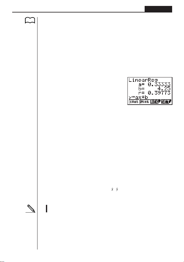
123
Statistical Graphs and Calculations Chapter 7
P. 1 1 8
Now you can press f and c to view variable characteristics.
For details on the meanings of these statistical values, see “Displaying Paired-Vari-
able Statistical Results”.
kk
kk
k Regression Calculation
In the explanations from "Linear Regression Graph" to "Power Regression Graph,"
regression calculation results were displayed after the graph was drawn. Here, the
regression line and regression curve is represented by mathematical expressions.
You can directly determine the same expression from the data input screen.
Perform the following key operation.
2(CALC)3(REG)
1(X)
Single variable regression parameters are displayed.
Next, you can use the following.
1 (X) ............ Linear regression
2 (Med) ........ Med-Med regression
3 (X^2) ......... Quadratic regression
[
1 (Log) ......... Logarithmic regression
2 (Exp) ......... Exponential regression
3 (Pwr) ......... Power regression
The meaning of the parameters that appear on this screen are the same as those for
“Linear Regression Graph” to “Power Regression Graph”.
kk
kk
k Estimated Value Calculation ( , )
After drawing a regression graph with the STAT Mode, you can use the RUN Mode
to calculate estimated values for the regression graph's
x and y parameters.
•Note that you cannot obtain estimated values for Med-Med graph and quad-
ratic regression graph.
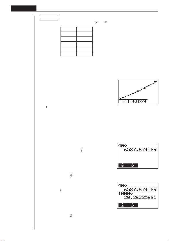
124
Chapter 7 Statistical Graphs and Calculations
(G-Type)
(Scat)
(XList)
(YList)
(Freq)
(M-Type)
(Auto)
(Pwr)
1234
Example To perform power regression using the following data and
estimate the values of
and when xi = 40 and yi = 1000
xi (List 1) yi (List 2)
28 2410
30 3033
33 3895
35 4491
38 5717
1. In the Main Menu, select the STAT icon and enter the STAT Mode.
2. Input data into the list and draw the power regression graph.
1(GRPH)[4(SET)c
1(Scat)c
1(List1)c
2(List2)c
1(1)c
1(
)Q
!Z1(Auto)Q1(GRPH)1(GPH1)[
3(Pwr)4(DRAW)
3. In the Main Menu, select the RUN icon and enter the RUN Mode.
4. Press the keys as follows.
ea(value of
xi)
K3(STAT)2( )w
The estimated value
is displayed for xi = 40.
baaa(value of
yi)
1( )w
The estimated value
is displayed for yi = 1000.

Programming
1. Before Programming
2. Programming Examples
3. Debugging a Program
4. Calculating the Number of Bytes Used by a Program
5. Secret Function
6. Searching for a File
7. Editing Program Contents
8. Deleting a Program
9. Useful Program Commands
10. Command Reference
11. Text Display
12. Using Calculator Functions in Programs
Chapter
8

126
Chapter 8 Programming
1. Before Programming
The programming function helps to make complex, often-repeated calculations quick
and easy. Commands and calculations are executed sequentially, just like the manual
calculation multistatements. Multiple programs can be stored under file names for
easy recall and editing.
Select the PRGM icon in the Main Menu and enter the PRGM Mode. When you do,
a program list appears on the display.
Selected memory area
(use
f
and
c
to move)
1 (EXE) ........ Execute program
2 (EDIT) ....... Program edit
3 (NEW) ...... New program
[
1 (DEL) ........ Specific program delete
2 (DEL•A) .... Delete all
3 (SRC) ....... File name search
Press [ to return to the previous menu.
• If there are not programs stored in memory when you enter the PRGM Mode, the
message “No Programs” appears on the display and only the NEW item (3) is
shown in the function menu.
File Name
Program
File Name
Program
File Name
Program
1234 [
1234 [
P. 138
P. 138
P. 135

127
Programming Chapter 8
A
1234
2. Programming Examples
Example 1To calculate the surface area and volume of three regular
octahedrons of the dimensions shown in the table below
Store the calculation formula under the file name OCTA.
Length of One Side (A) Surface Area (S) Vo lume (V)
7 cm cm
2
cm
3
10 cm cm
2
cm
3
15 cm cm
2
cm
3
The following are the formulas used for calculating surface area S and volume V of a
regular octahedron for which the length of one side is known.
2
S = 2
3 A
2
,V = –––– A
3
3
When inputting a new formula, you first register the file name and then input the
actual program.
uu
uu
uTo register a file name
Example To register the file name OCTA
•Note that a file name can be up to eight characters long.
1. While the program list is on the display, press 3 (NEW).
3(NEW)
3 (Q) .......... Password registration
4 (SYBL)...... Symbol menu
2. Input the name of the file.
OCTA
• The cursor changes form to indicate alpha character input.
• The following are the characters you can use in a file name:
A through Z, spaces, [, ], {, }, ’, ”, ~, 0 through 9, ., +, –, ×, ÷
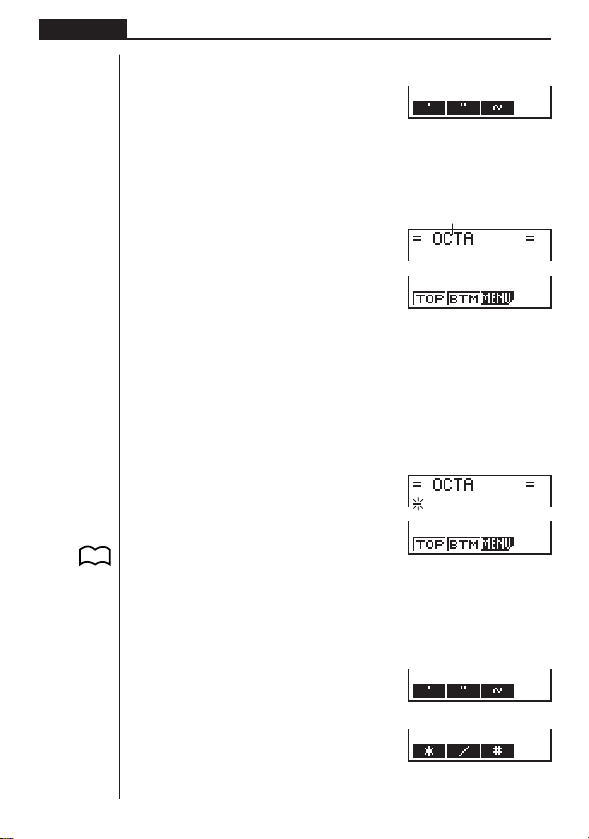
128
Chapter 8 Programming
•Pressing 4 (SYBL) displays a menu of symbols that can be input.
4(SYBL)
•You can delete a character while inputting a file name by moving the cursor to the
character you want to delete and pressing D.
3. Press w to register the file name and change to the program input screen.
w
•Registering a file name uses 17 bytes of memory.
• The file name input screen remains on the display if you press w without input-
ting a file name.
•To exit the file name input screen and return to the program list without register-
ing a file name, press Q.
uu
uu
uTo input a program
Use the program input screen to input the contents of a program.
1 (TOP) ........ Top of program
2 (BTM) ....... Bottom of program
3 (MENU) .... Mode menu
•Pressing [ displays a menu of symbols that can be input into a program.
[
[
Press [ to return to the previous menu.
1234
File name
P. 136
P. 136
1234 [
1234 [
1234 [
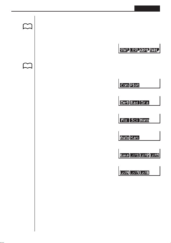
129
Programming Chapter 8
uu
uu
uTo change modes in a program
•Pressing 3 (MENU) while the program input screen is on the display causes a
mode change menu to appear. You can use this menu to input mode changes into
your programs. For details on each of these modes, see “Using the Main Menu”, as
well as the sections of this manual that describe what you can do in each mode.
3(MENU)
•Pressing ! Z displays a menu of commands that can be used to change set
up screen settings inside a program. For details on each of these commands, see
“To change a mode set up”.
!Z
[
[
[
[
[
Actual program contents are identical to manual calculations. The following shows
how the calculation of the surface area and volume of a regular octahedron would be
calculated using a manual calculation.
Surface Area S ... c*!9d* <value of A> xw
Volume V ............ !9c/d* <value of A> Mdw
You could also perform this calculation by assigning the value for the length of one
side to variable A.
Length of One Side A
............. <value of A> aaAw
P. 2
P. 6
1234
1234[
1234 [
1234 [
1234[
1234[
1234 [
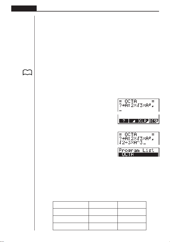
130
Chapter 8 Programming
Surface Area S ... c*!9d*aAxw
Volume V ............ !9c/d*aAMdw
If you simply input the manual calculations shown above however, the calculator
would execute them from beginning to end, without stopping. The following com-
mands make it possible to interrupt a calculation for input of values and display of
intermediate results.
?: This command pauses program execution and displays a question mark as a
prompt for input of a value to assign to a variable. The syntax for this command
is: ? → <variable name>.
^^
^^
^: This command pauses program execution and displays the last calculation re-
sult obtained or text. It is similar to pressing w in a manual calculation.
• For full details on using these and other commands, see “Useful Program Com-
mands”.
The following shows examples of how to actually use the ? and ^ commands.
!W[1(?)aaA[3(:)
c*!9d*aAx
[[2(^)
!9c/d*aAMd
QQ
uu
uu
uTo run a program
1. While the program list is on the display, use f and c to highlight the name of
the program you want to run.
2. Press 1 (EXE) or w to run the program.
Let’s try running the program we input above.
Length of One Side (A) Surface Area (S) Vo lume (V)
7 cm 169.7409791 cm
2
161.6917506 cm
3
10 cm 346.4101615 cm
2
471.4045208 cm
3
15 cm 779.4228634 cm
2
1590.990258 cm
3
P. 139
1234
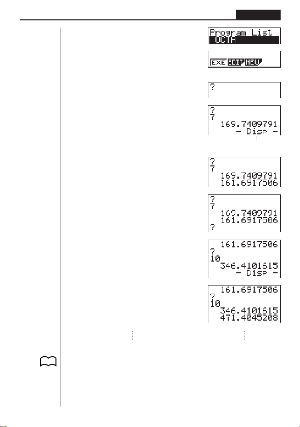
131
Programming Chapter 8
1 (EXE) or w
hw
(Value of A)
Intermediate result produced by
^
w
w
baw
w
•Pressing w while the program’s final result is on the display re-executes the
program.
•You can also run a program while in the RUN Mode by inputting:
Prog ”<file name>” w.
•An error (Go ERROR) occurs if the program specified by Prog ”<file name>”
cannot be found.
1 234
P. 149

132
Chapter 8 Programming
3. Debugging a Program
A problem in a program that keeps the program from running correctly is called a
“bug,” and the process of eliminating such problems is called “debugging.” Either of
the following symptoms indicates that your program contains bugs and that debug-
ging is required.
•Error messages appearing when the program is run
•Results that are not within your expectations
uu
uu
uTo eliminate bugs that cause error messages
An error message, like the one shown below, appears whenever something illegal
occurs during program execution.
When such a message appears, press d or e to display the location where the
error was generated, along with the cursor. Check the “Error Message Table” for
steps you should take to correct the situation.
•Note that pressing d or e will not display the location of the error if the pro-
gram is password protected.
uu
uu
uTo eliminate bugs that cause bad results
If your program produces results that are not what you normally expect, check the
contents of the program and make necessary changes. See “Editing Program Con-
tents” for details on how to change program contents.
4. Calculating the Number of Bytes Used
by a Program
This unit comes with 20,000 bytes of memory. A byte is a unit of memory that can be
used for storage of data.
There are two types of commands: 1-byte commands and 2-byte commands.
• Examples of 1-byte commands: sin, cos, tan, log, (, ), A, B, C, 1, 2, etc.
• Examples of 2-byte commands: Lbl 1, Goto 2, etc.
While the cursor is located inside of a program, each press of d or e causes the
cursor to move one byte.
•You can check how much memory has been used and how much remains at any
time by selecting the MEM icon in the Main Menu and entering the MEM Mode.
See “Memory Status (MEM)” for details.
P.200
P. 135
P. 3 7
P. 133
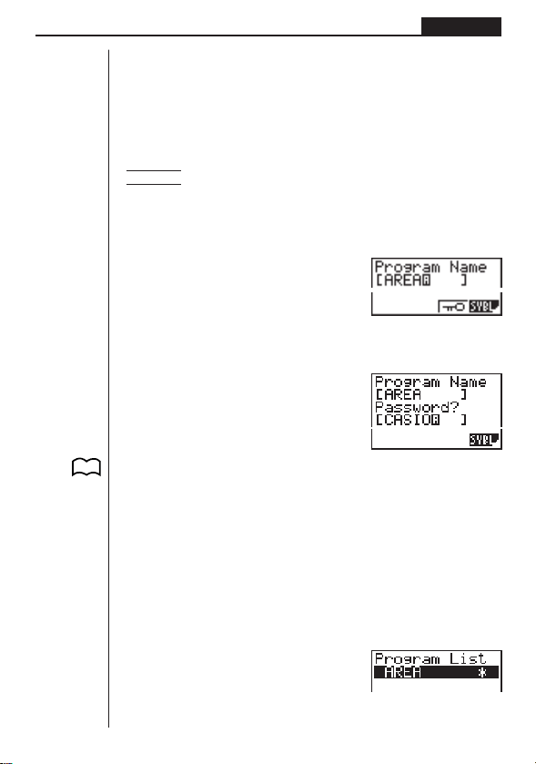
133
Programming Chapter 8
5. Secret Function
When inputting a program, you can protect it with a password that limits access to
the program contents to those who know the password. Password protected pro-
grams can be executed by anyone without inputting the password.
uu
uu
uTo register a password
Example To create a program file under the name AREA and protect it with
the password CASIO
1. While the program list is on the display, press 3 (NEW) and input the file name
of the new program file.
3(NEW)
AREA
2. Press 3 (Q) and then input the password.
3(Q)
CASIO
• The password input procedure is identical to that used for file name input.
3. Press w to register the file name and password. Now you can input the contents
of the program file.
•Registration of a password uses 16 bytes of memory.
•Pressing w without inputting a password registers the file name only, without a
password.
4. After inputting the program, press Q to exit the program file and return to the
program list. Files that are password protected are indicated by an asterisk to the
right of the file name.
Q
P. 127
1233 56
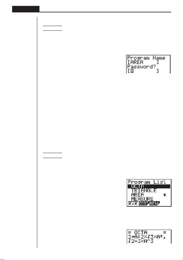
134
Chapter 8 Programming
uu
uu
uTo recall a program
ExampleTo recall the file named AREA which is protected by the
password CASIO
1. In the program list, use f and c to move the highlighting to the name of the
program you want to recall.
2. Press 2 (EDIT).
2(EDIT)
3. Input the password and press w to recall the program.
• The message “Mismatch” appears if you input the wrong password.
6. Searching for a File
You can search for a specific file name using any of the three following methods.
•Scroll Search — scroll through the file names in the program list.
•File Name Search — input the name of the file.
•Initial Character Search — input the first few letters of the name of the file.
uu
uu
uTo find a file using scroll search
Example To use scroll search to recall the program named OCTA
1. While the program list is on the display, use f and c to scroll through the list
of program names until you find the one you want.
2. When the highlighting is located at the name of the file you want, press 2 (EDIT)
to recall it.
2(EDIT)
1 2 34
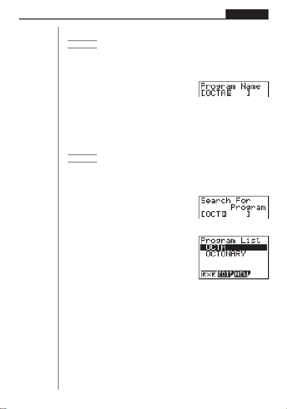
135
Programming Chapter 8
uu
uu
uTo find a file using file name search
Example To use file name search to recall the program named OCTA
1. While the program list is on the display, press 3 (NEW) and input the name of
the file you want to find.
3(NEW)
OCTA
2. Press w to recall the program.
• If there is no program whose file name matches the one you input, a new file is
created using the input name.
uu
uu
uTo find a file using initial character search
Example To use initial character search to recall the program named OCTA
1. While the program list is on the display, press [ 3 (SRC) and input the initial
characters of the file you want to find.
[3(SRC)
OCT
2. Press w to search.
w
•All files whose file names start with the characters you input are recalled.
• If there is no program whose file name starts with the characters you input, the
message “Not Found” appears on the display. If this happens, press Q to clear
the error message.
3. Use f and c to highlight the file name of the program you want to recall and
then press 2 (EDIT) to recall it.
7. Editing Program Contents
uu
uu
uTo edit program contents
1. Find the file name of the program you want in the program list.
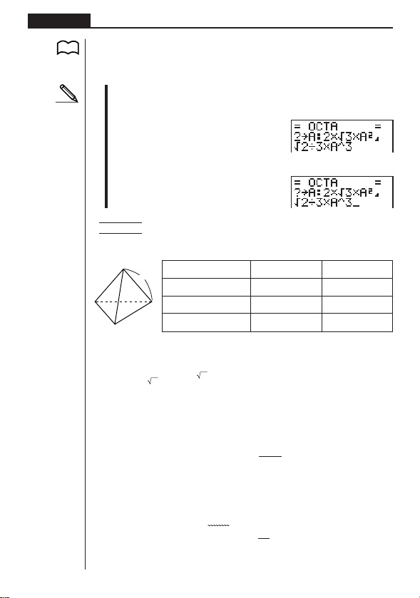
136
Chapter 8 Programming
2. Recall the program.
• The procedures you use for editing program contents are identical to those used
for editing manual calculations. For details, see “Making Corrections”.
• The following function keys are also useful when editing program contents.
1 (TOP) ........ Moves the cursor to the top of the program
2 (BTM) ....... Moves the cursor to the bottom of the program
Example 2
To use the OCTA program to create a program that calculates
the surface area and volume of regular tetrahedrons when the
length of one side is known
Length of One Side (A) Surface Area (S) Vo lume (V)
7 cm cm
2
cm
3
10 cm cm
2
cm
3
15 cm cm
2
cm
3
The following are the formulas used for calculating surface area S and volume V of a
regular tetrahedron for which the length of one side is known.
2
S =
3 A
2
,V = –––– A
3
12
Use the following key operations when inputting the program.
Length of One Side A .. !W[1(?)aaA[3(:)
Surface Area S ............ !9d*aAx[[2(^)
Volume V ..................... !9c/bc*aAMd
Compare this with the program for calculating the surface area and volume of a
regular octahedron.
Length of One Side A .. !W[1(?)aaA[3(:)
Surface Area S ............ c*!9d*aAx[[2(^)
Volume V ..................... !9c/d*aAMd
P. 2 0
A
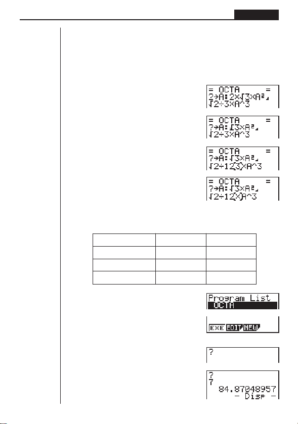
137
Programming Chapter 8
As you can see, you can produce the TETRA program by making the following changes
in the OCTA program.
•Deleting c * (underlined using a wavy line above)
•Changing d to b c (underlined using a solid line above)
Let’s edit the program.
2(EDIT)
eeeeDD
cd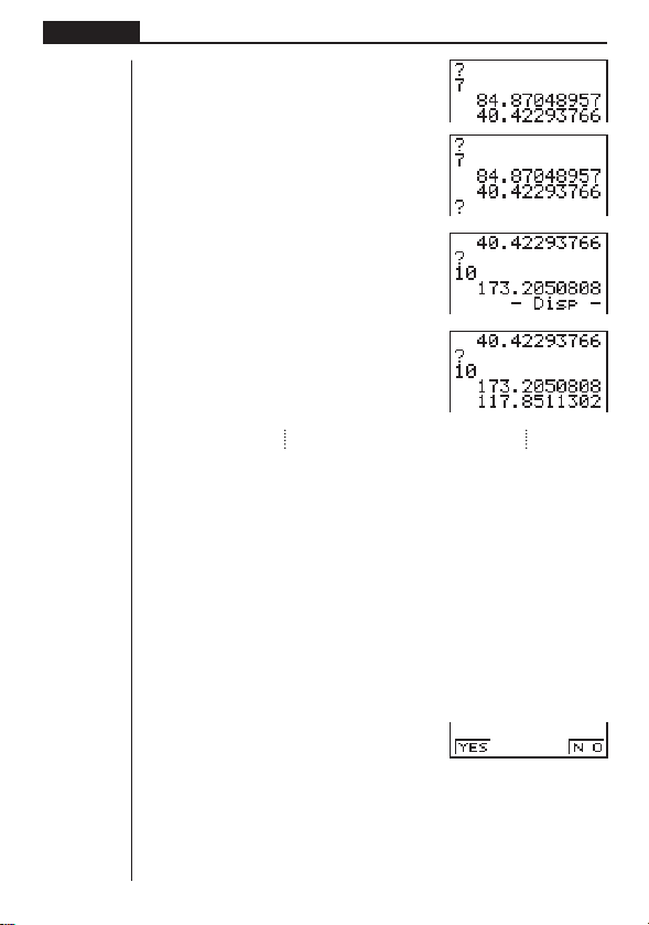
138
Chapter 8 Programming
w
w
baw
w
8. Deleting a Program
There are two different ways to delete a file name and its program.
•Specific program delete
•All program delete
uu
uu
uTo delete a specific program
1. While the program list is on the display, use f and c to move the highlighting
to the name of the program you want to delete.
2. Press [ 1 (DEL).
[1(DEL)
3. Press 1 (YES) to delete the selected program or 4 (NO) to abort the opera-
tion without deleting anything.
uu
uu
uTo delete all programs
1. While the program list is on the display, press [ 2 (DEL•A).
1 234

139
Programming Chapter 8
[2(DEL•A)
2. Press 1 (YES) to delete all the programs in the list or 4 (NO) to abort the
operation without deleting anything.
•You can also delete all programs using the MEM Mode. See “Clearing Memory
Contents” for details.
9. Useful Program Commands
In addition to calculation commands, this calculator also includes a variety of rela-
tional and jump commands that can be used to create programs that make repeat
calculations quick and easy.
Program Menu
Press ! W to display the program menu.
!W
1 (COM) ...... Program command menu
2 (CTL) ........ Control command menu
3 (JUMP) ..... Jump command menu
[
1 (?) ............. Input command
2 (^) ........... Output command
3 (CLR) ........ Clear command menu
4 (DISP) ...... Display command menu
[
1 (REL) ........ Conditional jump relational operator menu
2 (I/O) .......... Input/output command menu
3 (:) .............. Multi-statement command
Press [ to return to the previous menu.
1 234
1234 [
1234[
1234 [
P. 3 7
P. 140
P. 140
P. 141
P. 141
P. 141
P. 142
P. 142
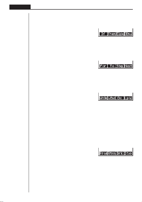
140
Chapter 8 Programming
Program Command Menu (COM)
While the program menu is on the display, press 1 (COM) to display the program
command menu.
1(COM)
1 (If) ............. If command
2 (Then) ....... Then command
3 (Else) ........ Else command
4 (I•End) ...... IfEnd command
[
1 (For) .......... For command
2 (To) ........... To command
3 (Step) ....... Step command
4 (Next) ........ Next command
[
1 (Whle) ....... While command
2 (WEnd) ..... WhileEnd command
3 (Do) .......... Do command
4 (Lp•W) ...... LpWhile command
Press [ to return to the previous menu.
Control Command Menu (CTL)
While the program menu is on the display, press 2 (CTL) to display the control
command menu.
2(CTL)
1 (Prog) ....... Prog command
2 (Rtrn) ........ Return command
3 (Brk) ......... Break command
4 (Stop) ....... Stop command
1 234[
1234
1 234[
1 234[
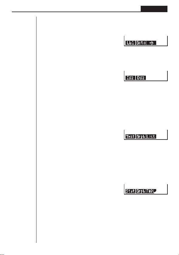
141
Programming Chapter 8
Jump Command Menu (JUMP)
While the program menu is on the display, press 3 (JUMP) to display the jump
command menu.
3(JUMP)
1 (Lbl) .......... Lbl command
2 (Goto) ....... Goto command
3 (⇒) ........... ⇒ (jump) command
[
1 (Isz) .......... Isz command
2 (Dsz) ......... Dsz command
Press [ to return to the previous menu.
Clear Command Menu (CLR)
While the program menu is on the display, press [ 3 (CLR) to display the clear
command menu.
[3(CLR)
1 (Text) ........ ClrText command
2 (Grph) ....... ClrGraph command
3 (List) ......... ClrList command
Display Command Menu (DISP)
While the program menu is on the display, press [ 4 (DISP) to display the dis-
play command menu.
[4(DISP)
1 (Stat) ........ DrawStat command
2 (Grph) ....... DrawGraph command
3 (TABL) ...... Table & Graph command menu
Pressing 3 (TABL) while the display command menu is on the display causes the
Table & Graph command menu to appear.
1234[
1234
1234 [
1234
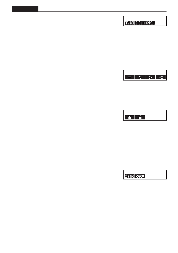
142
Chapter 8 Programming
3(TABL)
1 (Tabl) ........ DispTable command
2 (G•Con) .... DrawTG-Con command
3 (G•Plt)....... DrawTG-Plt command
Conditional Jump Relational Operator Menu (REL)
While the program menu is on the display, press [ [ 1 (REL) to display the
conditional jump relational operator menu.
[[1(REL)
1 (=) ............. Relational operator =
2 (
GG
GG
G
)............. Relational operator
GG
GG
G
3 (>) ............. Relational operator >
4 (<) ............. Relational operator <
[
1 (≥) ............. Relational operator ≥
2 (≤) ............. Relational operator ≤
Press [ to return to the previous menu.
Input/Output Commands Menu (I/O)
While the program menu is on the display, press [[2 (I/O) to display the input/
output command menu.
[[2(I/O)
1 (Send) ...... Send ( command
2 (Recv) ....... Receive ( command
1234
1234[
1234[
1234[

143
Programming Chapter 8
10. Command Reference
kk
kk
k Command Index
Break .................................................................................... 149
ClrGraph ............................................................................... 153
ClrList.................................................................................... 153
ClrText ................................................................................... 153
DispTable .............................................................................. 154
Do~LpWhile ........................................................................... 148
DrawTG-Con, DrawTG-Plt ..................................................... 154
DrawGraph ............................................................................154
DrawStat ............................................................................... 153
Dsz ........................................................................................ 151
For~To~Next ..........................................................................147
For~To~Step~Next ................................................................ 147
Goto~Lbl ............................................................................... 151
If~Then ................................................................................. 145
If~Then~Else .........................................................................146
If~Then~Else~IfEnd ............................................................... 146
If~Then~IfEnd ........................................................................ 145
Isz ......................................................................................... 152
Prog ...................................................................................... 149
Receive( ................................................................................ 154
Return ................................................................................... 150
Send( .................................................................................... 155
Stop ...................................................................................... 150
While~WhileEnd ....................................................................148
? (Input Command) ................................................................ 144
^ (Output Command) ........................................................... 144
: (Multi-statement Command) ................................................ 144
_ (Carriage Return) ............................................................. 144
⇒ (Jump Code) .....................................................................152
=,
GG
GG
G
, >, <, ≥, ≤ (Relational Operators) ................................... 155
The following are conventions that are used in this section when describing the vari-
ous commands.
Boldface Text .............. Actual commands and other items that always must be in-
put are shown in boldface.
{Curly Brackets} ......... Curly brackets are used to enclose a number of items, one
of which must be selected when using a command. Do not
input the curly brackets when inputting a command.

144
Chapter 8 Programming
[Square Brackets] ....... Square brackets are used to enclose items that are op-
tional. Do not input the square brackets when inputting a
command.
Numeric Expressions . Numeric expressions (such as 10, 10 + 20, A) indicate con-
stants, calculations, numeric constants, etc.
Alpha Characters ....... Alpha characters indicate literal strings (such as AB).
kk
kk
k Basic Operation Commands
? (Input Command)
Function: Prompts for input of values for assignment to variables during program
execution.
Syntax: ? → <variable name>
Example: ? → A _
Description:
1. This command momentarily interrupts program execution and prompts for input
of a value or expression for assignment to a variable. When the input command is
executed, “?” to appears on the display and the calculator stands by for input.
2. Input in response to the input command must be a value or an expression, and
the expression cannot be a multi-statement.
^^
^^
^ (Output Command)
Function: Displays and intermediate result during program execution.
Description:
1. This command momentarily interrupts program execution and displays alpha
character text or the result of the calculation immediately before it.
2. The output command should be used at locations where you would normally
press the w key during a manual calculation.
: (Multi-statement Command)
Function: Connects two statements for sequential execution without stopping.
Description:
1. Unlike the output command (^), statements connected with the multi-statement
command are executed non-stop.
2. The multi-statement command can be used to link two calculation expressions or
two commands.
3. You can also use a carriage return indicated by _ in place of the multi-statement
command.
__
__
_ (Carriage Return)
Function: Connects two statements for sequential execution without stopping.

145
Programming Chapter 8
Description:
1. Operation of the carriage return is identical to that of the multi-statement com-
mand.
2. Using a carriage return in place of the multi-statement command makes the dis-
played program easier to read.
kk
kk
k Program Commands (COM)
If~Then
Function: The Then-statement is executed only when the If-condition is true (non-
zero).
Syntax:
Parameters: condition, numeric expression
Description:
1. The Then-statement is executed only when the If-condition is true (non-zero).
2. If the condition is false (0), the Then-statement is not executed.
3. An If-condition must always be accompanied by a Then-statement. Omitting the
Then-statement results in an error (Syn ERROR).
Example: If A = 0 _
Then ”A = 0”
If~Then~IfEnd
Function: The Then-statement is executed only when the If-condition is true (non-
zero). The IfEnd-statement is always executed: after the Then-statement is executed
or directly after the If-condition when the If-condition is false (0).
Syntax:
Parameters: condition, numeric expression
Description:
This command is almost identical to If~Then. The only difference is that the IfEnd-
statement is always executed, regardless of whether the If-condition is true (non-
zero) or false (0).
Example: If A = 0 _
Then ”A = 0” _
IfEnd_
”END”
If
<condition>
_
:
^
Then <statement>
numeric expression
_
:
^
<statement>
_
:
^
IfEnd
__
If
<condition> : Then <statement> : <statement>
numeric expression
^^

146
Chapter 8 Programming
If~Then~Else
Function: The Then-statement is executed only when the If-condition is true (non-
zero). The Else-statement is executed when the If-condition is false (0).
Syntax:
Parameters: condition, numeric expression
Description:
1. The Then-statement is executed when the If-conditions is true (non-zero).
2. The Else-statement is executed when the If-conditions is false (zero).
Example: If A = 0 _
Then ”TRUE” _
Else ”FALSE”
If~Then~Else~IfEnd
Function: The Then-statement is executed only when the If-condition is true (non-
zero). The Else-statement is executed when the If-condition is false (0). The IfEnd-
statement is always executed following either the Then-statement or Else-statement.
Syntax:
Parameters: condition, numeric expression
Description:
This command is almost identical to If~Then~Else. The only difference is that the
IfEnd-statement is always executed, regardless of whether the If-condition is true
(non-zero) or false (0).
Example: ? → A _
If A = 0 _
Then ”TRUE”_
Else ”FALSE”_
IfEnd_
”END”
If
<condition>
_
:
^
Then <statement>
_
:
^
<statement>
numeric expression
_
:
^
Else <statement>
_
:
^
<statement>
If <condition>
_
:
^
Then <statement>
_
:
^
<statement>
numeric expression
_
:
^
Else <statement>
_
:
^
<statement>
_
:
^
IfEnd
147
Programming Chapter 8
For~To~Next
Function: This command repeats everything between the For-statement and the
Next-statement. The starting value is assigned to the control variable with the first
execution, and the value of the control variable is incremented by one with each
execution. Execution continues until the value of the control variable exceeds the
ending value.
Syntax:
Parameters:
• control variable name: A to Z
•starting value: value or expression that produces a value (i.e. sin
x, A, etc.)
• ending value: value or expression that produces a value (i.e. sin
x, A, etc.)
Description:
1. When the starting value of the control variable is greater than the ending value,
execution continues from the statement following Next, without executing the state-
ments between For and Next.
2. A For-statement must always have a corresponding Next-statement, and the Next-
statement must always come after its corresponding For-statement.
3. The Next-statement defines the end of the loop created by For~Next, and so it
must always be included. Failure to do so results in an error (Syn ERROR).
Example: For 1 → A To 10_
A × 3 → B_
B ^
Next
For~To~Step~Next
Function: This command repeats everything between the For-statement and the
Next-statement. The starting value is assigned to the control variable with the first
execution, and the value of the control variable is changed according to the step
value with each execution. Execution continues until the value of the control variable
exceeds the ending value.
Syntax:
Parameters:
• control variable name: A to Z
•starting value: value or expression that produces a value (i.e. sin
x, A, etc.)
• ending value: value or expression that produces a value (i.e. sin
x, A, etc.)
•step value: numeric value (omitting this value sets the step to 1)
_
For
<starting value> → <control variable name>
To
<ending value>
:
^
_
<statement>
: Next
^
_
For
<starting value> → <control variable name>
To
<ending value>
Step
<step value>
:
^
Next

148
Chapter 8 Programming
_
Do
: ~ LpWhile <expression>
^
_
While <expression>
: ~WhileEnd
^
Description:
1. This command is basically identical to For~To~Next. The only difference is that
you can specify the step.
2. Omitting the step value automatically sets the step to 1.
3. Making the starting value less than the ending value and specifying a positive
step value causes the control variable to be incremented with each execution.
Making the starting value greater than the ending value and specifying a negative
step value causes the control variable to be decremented with each execution.
Example: For 1 → A To 10 Step 0.1_
A × 3 → B _
B ^
Next
Do~LpWhile
Function: This command repeats specific commands as long as its condition is true
(non-zero).
Syntax:
Parameters: expression
Description:
1. This command repeats the commands contained in the loop as long as its condi-
tion is true (non-zero). When the condition becomes false (0), execution pro-
ceeds from the statement following the LpWhile-statement.
2. Since the condition comes after the LpWhile-statement, the condition is tested
(checked) after all of the commands inside the loop are executed.
Example: Do_
? → A_
A × 2 → B_
B ^
LpWhile B >10
While~WhileEnd
Function: This command repeats specific commands as long as its condition is true
(non-zero).
Syntax:
Parameters: expression

149
Programming Chapter 8
Description:
1. This command repeats the commands contained in the loop as long as its condi-
tion is true (non-zero). When the condition becomes false (0), execution pro-
ceeds from the statement following the WhileEnd-statement.
2. Since the condition comes after the While-statement, the condition is tested
(checked) before the commands inside the loop are executed.
Example: 10 → A_
While A > 0_
A – 1 → A_
”GOOD”_
WhileEnd
kk
kk
k Program Control Commands (CTL)
Break
Function: This command breaks execution of a loop and continues from the next
command following the loop.
Syntax: Break _
Description:
1. This command breaks execution of a loop and continues from the next command
following the loop.
2. This command can be used to break execution of a For-statement, Do-state-
ment, and While-statement.
Example: While A>0_
If A > 2_
Then Break_
IfEnd_
WhileEnd_
A ^ ← Executed after Break
Prog
Function: This command specifies execution of another program as a subroutine. In
the RUN Mode, this command executes a new program.
Syntax: Prog ”file name” _
Example: Prog ”ABC” _
Description:
1. Even when this command is located inside of a loop, its execution immediately
breaks the loop and launches the subroutine.
2. This command can be used as many times as necessary inside of a main routine
to call up independent subroutines to perform specific tasks.
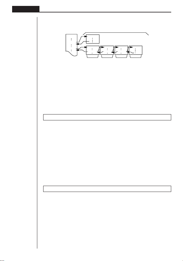
150
Chapter 8 Programming
3. A subroutine can be used in multiple locations in the same main routine, or it can
be called up by any number of main routines.
D
CEIJ
Prog ”E” Prog ”I” Prog ”J”
A
Prog ”D”
Prog ”C”
4. Calling up a subroutine causes it to be executed from the beginning. After execu-
tion of the subroutine is complete, execution returns to the main routine, continu-
ing from the statement following the Prog command.
5. A Goto~Lbl command inside of a subroutine is valid inside of that subroutine only.
It cannot be used to jump to a label outside of the subroutine.
6. If a subroutine with the file name specified by the Prog command does not exist,
an error (Go ERROR) occurs.
7. In the RUN Mode, inputting the Prog command and pressing w launches the
program specified by the command.
Return
Function: This command returns from a subroutine.
Syntax: Return _
Description:
Execution of the Return command inside a main routine causes execution of the
program to stop.
Example: Prog ”A” Prog ”B”
1 → A_ For A → B To 10_
Prog ”B”_ B + 1 → C_
C ^ Next_
Return
Executing the program in File A displays the result of the operation (11).
Stop
Function: This command terminates execution of a program.
Syntax: Stop _
Description:
1. This command terminates program execution.
2. Execution of this command inside of a loop terminates program execution with-
out an error being generated.
Level 1 Level 2 Level 3 Level 4
Main Routine Subroutines

151
Programming Chapter 8
Example: For 2 → I To 10_
If I = 5_
Then ”STOP” : Stop_
IfEnd_
Next
This program counts from 2 to 10. When the count reaches 5, however, it terminates
execution and displays the message ”STOP.”
kk
kk
k Jump Commands (JUMP)
Dsz
Function: This command is a count jump that decrements the value of a control
variable by 1, and then jumps if the current value of the variable is zero.
Syntax:
Parameters:
Variable Name: A to Z
[Example] Dsz B : Decrements the value assigned to variable B by 1.
Description:
This command decrements the value of a control variable by 1, and then tests (checks)
it. If the current value is non-zero, execution continues with the next statement. If the
current value is zero, execution jumps to the statement following the multi-statement
command (:), display command (^), or carriage return (_).
Example: 10 → A : 0 → C :
Lbl 1 : ? → B : B+C → C :
Dsz A : Goto 1 : C ÷ 10
This program prompts for input of 10 values, and then calculates the
average of the input values.
Goto~Lbl
Function: This command performs an unconditional jump to a specified location.
Syntax: Goto <value or variable> ~ Lbl <value or variable>
Parameters: Value (from 0 to 9), variable (A to Z)
Description:
1. This command consists of two parts: Goto
n (where n is a value from 0 to 9) and
Lbl
n (where n is the value specified for Goto). This command causes program
execution to jump to the Lbl-statement whose value matches that specified by
the Goto-statement.
2. This command can be used to loop back to the beginning of a program or to jump
to any location within the program.
Variable Value
GG
GG
G
0
_
Dsz <variable name> : <statement>
: <statement>
^
Variable Value = 0
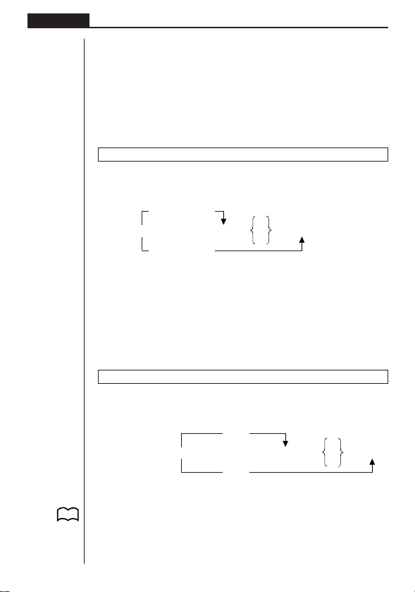
152
Chapter 8 Programming
3. This command can be used in combination with conditional jumps and count
jumps.
4. If there is no Lbl-statement whose value matches that specified by the Goto-
statement, an error (Go ERROR) occurs.
Example: ? → A : ? → B : Lbl 1 :
? → X : A × X + B ^
Goto 1
This program calculates
y = AX + B for as many values for each variable that you
want to input. To quit execution of this program, press A.
Isz
Function: This command is a count jump that increments the value of a control
variable by 1, and then jumps if the current value of the variable is zero.
Syntax:
Parameters:
Variable Name: A to Z
[Example] Isz A : Increments the value assigned to variable A by 1.
Description:
This command increments the value of a control variable by 1, and then tests (checks)
it. If the current value is non-zero, execution continues with the next statement. If the
current value is zero, execution jumps to the statement following the multi-statement
command (:), display command (^), or carriage return (_).
⇒ (Jump Code)
Function: This code is used to set up conditions for a conditional jump. The jump is
executed whenever the conditions are false.
Syntax:
Parameters:
left side/right side: variable (A to Z), numeric constant, variable expression (such as:
A × 2)
relational operator: =,
GG
GG
G
, >, <, ≥, ≤
P. 155
True
_
<left side> <relational operator> <right side> ⇒ <statement>
:
<statement>
^
False
Va r i able Value
GG
GG
G
0
_
Isz <variable name> : <statement> : <statement>
^
Variable Value = 0

153
Programming Chapter 8
Description:
1. The conditional jump compares the contents of two variables or the results of two
expressions, and a decision is made whether or not to execute the jump based
on the results of the comparison.
2. If the comparison returns a true result, execution continues with the statement
following the ⇒ command. If the comparison returns a false result, execution
jumps to the statements following the multi-statement command (:), display com-
mand (^), or carriage return (_).
Example: Lbl 1 : ? → A :
A > 0 ⇒
A ^
Goto 1
With this program, inputting a value of zero or greater calculates and displays the
square root of the input value. Inputting a value less than zero returns to the input
prompt without calculating anything.
kk
kk
k Clear Commands (CLR)
ClrGraph
Function: This command clears the graph screen.
Syntax: ClrGraph_
Description: This command clears the graph screen during program execution.
ClrList
Function: This command clears list data.
Syntax: ClrList_
Description: This command clears the contents of the currently selected list (List 1
to List 6) during program execution.
ClrText
Function: This command clears the text screen.
Syntax: ClrText_
Description:
This command clears text from the screen during program execution.
kk
kk
k Display Commands (DISP)
DrawStat
Function: This draws a statistical graph.
Syntax:
DrawStat_

154
Chapter 8 Programming
Description:
This command draws a statistical graph in accordance with conditions defined within
the program.
DrawGraph
Function: This command draws a graph.
Syntax: DrawGraph_
Description: This command draws a graph in accordance with the drawing condi-
tions defined within the program.
DispTable
Function: These commands display numeric tables.
Syntax:
DispTable_
Description:
These commands generate numeric tables during program execution in accordance
with conditions defined within the program.
DrawTG-Con, DrawTG-Plt
Function: These commands graph functions.
Syntax:
DrawTG-Con_
DrawTG-Plt_
Description:
1. These commands graph functions in accordance with conditions defined within
the program.
2. DrawTG-Con produces a connect type graph, while DrawTG-Plt produces a plot
type graph.
kk
kk
k Input/Output Commands (I/O)
Receive (
Function: This command receives data from an external device.
Syntax: Receive (<data>) (…ex. Receive (List 1))
Description:
1. This command receives data from an external device.
2. The following types of data can be received by this command.
•Individual values assigned to variables
•List data (all values - individual values cannot be specified)

155
Programming Chapter 8
Send (
Function: This command sends data to an external device.
Syntax: Send (<data>) (…ex. Send (List 1))
Description:
1. This command sends data to an external device.
2. The following types of data can be sent by this command.
•Individual values assigned to variables
•List data (all values - individual values cannot be specified)
kk
kk
k Conditional Jump Relational Operators (REL)
=,
GG
GG
G
, >, <, ≥, ≤
Function: These relational operators are used in combination with the conditional
jump command.
Syntax:
Parameters:
left side/right side: variable (A to Z), numeric constant, variable expression (such as:
A × 2)
relational operator: =,
GG
GG
G
, >, <, ≥, ≤
Description:
1. The following six relational operators can be used in the conditional jump com-
mand
<left side> = <right side> : true when <left side> equals <right side>
<left side>
GG
GG
G
<right side> : true when <left side> does not equal <right side>
<left side> > <right side> : true when <left side> is greater than <right side>
<left side> < <right side> : true when <left side> is less than <right side>
<left side> ≥ <right side> : true when <left side> is greater than or equal to <right
side>
<left side> ≤ <right side> : true when <left side> is less than or equal to <right side>
2. See “⇒ (Jump Code)” for details on using the conditional jump.
_
<left side> <relational operator> <right side> ⇒ <statement>
:
<statement>
^
(With Jump Code)
P. 152

156
Chapter 8 Programming
11. Text Display
You can include text in a program by simply enclosing it between double quotation
marks. Such text appears on the display during program execution, which means
you can add labels to input prompts and results.
Program Display
? → X?
”X =” ? → XX = ?
• If the text is followed by a calculation formula, be sure to insert a display com-
mand (^) or multi-statement command (:) between the text and calculation.
•Inputting more than 13 characters causes the text to move down to the next line.
The screen scrolls automatically if the text causes the screen to become full.
12. Using Calculator Functions in
Programs
kk
kk
k Using Graph Functions in a Program
You can incorporate graph functions into a program to draw complex graphs and to
overlay graphs on top of each other. The following shows various types of syntax you
need to use when programming with graph functions.
• View Window
View Window –5, 5, 1, –5, 5, 1 _
• Graph function input
Y = Type_ ...... Specifies graph type.
”X
2
– 3” → Y1_
• Graph draw operation
DrawGraph_
Example Program
1
ClrGraph_
1
!W[32
2
View Window –10, 10, 2, –120, 150, 50_
2
!31Q
3
Y = Type_
3
3321Q
”X ^ 4–X ^ 3–24X
2
+ 4X + 80” → Y1_
4
J[21Q
5
G SelOn 1_
5
3311
6
DrawGraph
6
!W[42
4
P. 4 8

157
Programming Chapter 8
Executing this program produces the result shown here.
kk
kk
k Using Table & Graph Functions in a Program
Table & Graph functions in a program can generate numeric tables and perform
graphing operations. The following shows various types of syntax you need to use
when programming with Table & Graph functions.
• Table range setting
1 → FStart_
5 → FEnd_
1 → F pitch_
• Numeric table generation
DispTable_
• Graph draw operation
Connect type: DrawTG-Con_
Plot type: DrawTG-Plt_
Example Program
ClrGraph_
ClrText_
View Window 0, 6, 1, –2, 106, 20_
Y = Type_
”3X
2
– 2” → Y1_
1
T SelOn 1_
1
341Q
0 →
2
FStart_
2
J[31
6 →
3
FEnd_
3
2
1 →
4
Fpitch_
4
3Q
5
DispTable^
5
!W[431Q
6
DrawTG-Con
6
!W[432Q
P. 7 4
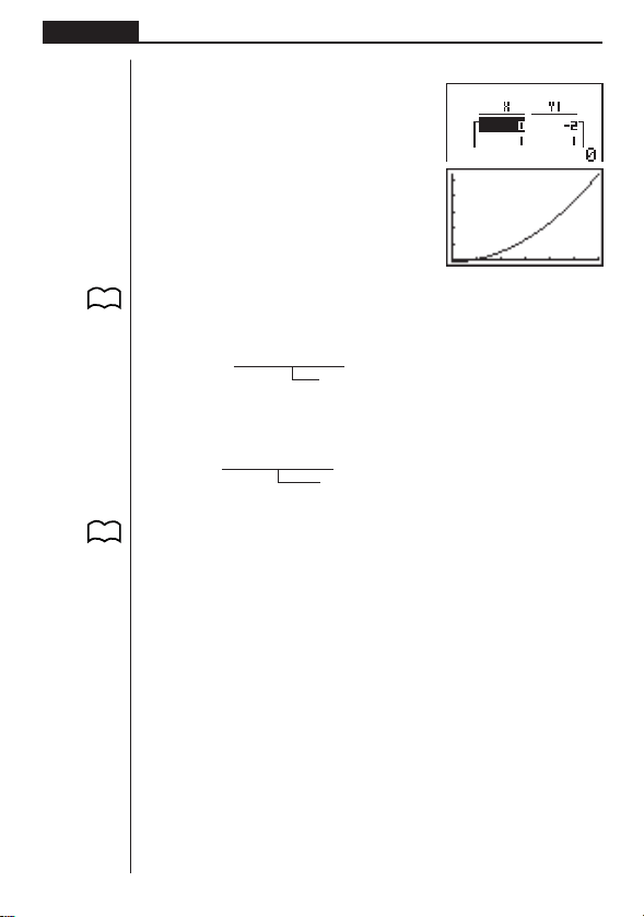
158
Chapter 8 Programming
Executing this program produces the results shown here.
Numeric Table
Graph
w
kk
kk
k Using List Sort Functions in a Program
These functions let you sort the data in lists into ascending or descending order.
• Ascending order
1
SortA (
2
List 1, List 2, List 3)
Lists to be sorted (up to six can be specified)
1
321Q
2
K11
• Descending order
SortD (List 1, List 2, List 3)
Lists to be sorted (up to six can be specified)
kk
kk
k Using Statistical Calculations and Graphs in a Program
Including statistical calculations and graphing operations into program lets you cal-
culate and graph statistical data.
uu
uu
uTo set conditions and draw a statistical graph
Following “StatGrph”, you must specify the following graph conditions:
• Graph draw/non-draw status (DrawOn/DrawOff)
• Graph Type
•
x-axis data location (list name)
•
y-axis data location (list name)
• Frequency data location (list name)
• Mark Type
P. 8 2
P. 9 6

159
Programming Chapter 8
The graph conditions that are required depends on the graph type. See “Changing
Graph Parameters”.
• The following is a typical graph condition specification for a scatter diagram or
xy line graph.
S-Gph1 DrawOn, Scatter, List1, List2, 1, Square_
In the case of an
xy line graph, replace “Scatter” in the above specification with
“
xyLine”.
• The following is a typical graph condition specification for a pie chart.
S-Gph1 DrawOn, Pie, List1, % (data display format)_
• The following is a typical graph condition specification for a stacked bar chart, bar
graph, or line graph.
Stacked bar chart: ......... S-Gph1 DrawOn, StackedBar, List1_
Bar graph: ...................... S-Gph1 DrawOn, Bar, List1_
Line graph: ..................... S-Gph1 DrawOn, LineG, List1_
• The following is a typical graph condition specification for a superimposed bar
and line graph.
S-Gph1 DrawOn, Both, List1 (bar graph list), List2 (line graph list),
Sep. G(AutoWin setting)_
• The following is a typical graph condition specification for a single-variable graph.
S-Gph1 DrawOn, Hist, List1, List2_
The same format can be used for the following types of graphs, by simply replac-
ing “Hist” in the above specification with the applicable graph type.
Histogram: ..................... Hist
Median Box: ................... MedBox
Normal Distribution: ....... N-Dist
• The following is a typical graph condition specification for a regression graph.
S-Gph1 DrawOn, Linear, List1, List2, List3_
The same format can be used for the following types of graphs, by simply replac-
ing “Linear” in the above specification with the applicable graph type.
Linear Regression: ........ Linear
Med-Med: ...................... Med-Med
Quadratic Regression: ... Quad
Logarithmic Regression: . Log
Exponential Regression: Exp
Power Regression : ....... Power
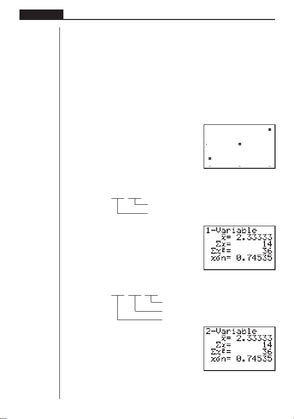
160
Chapter 8 Programming
Example Program
ClrGraph_
1
!Z[[[1Q
1
S-WindAuto_
2
K11
{1, 2, 3} →
2
List 1_
3
1Q
{1, 2, 3} →
3
List 2_
4
3121Q
4
S-Gph1
5
DrawOn,
5
3111Q
6
Scatter, List1, List2, 1,
7
Square_
6
312[1Q
8
DrawStat
7
3141Q
8
!W[41Q
Executing this program produces the scatter diagram shown here.
kk
kk
k Performing Statistical Calculations
• Single-variable statistical calculation
1
1-Variable List 1, List 2
Frequency data (Frequency)
x
-axis data (XList)
1
31[11Q
• Paired-variable statistical calculation
2-Variable List 1, List 2, List 3
Frequency data (Frequency)
y
-axis data (YList)
x
-axis data (XList)
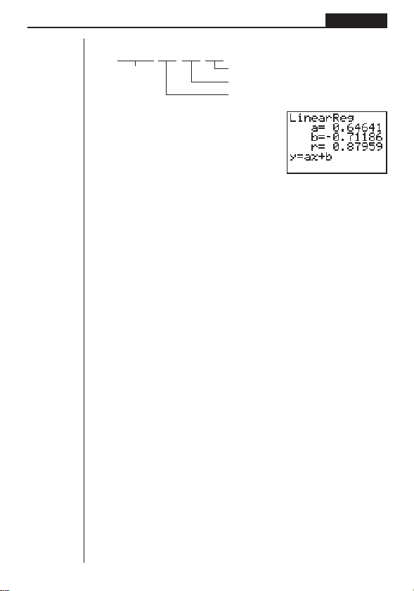
161
Programming Chapter 8
• Regression statistical calculation
1
LinearReg List 1, List 2, List 3
Calculation
Frequency data (Frequency)
type*
y
-axis data (YList)
x
-axis data (XList)
1
31[1[1Q
*Any one of the following can be specified as the calculation type.
LinearReg ....... linear regression
Med-MedLine .. Med-Med calculation
QuadReg ........ quadratic regression
LogReg ........... logarithmic regression
ExpReg ........... exponential regression
PowerReg ....... power regression

162
Chapter 8 Programming

Data Communications Chapter 9
163
Data Communications
This chapter tells you everything you need to know to transfer pro-
grams between the fx-7400G PLUS and certain CASIO Graphic Sci-
entific Calculator models connected with an optionally available SB-
62 cable. To transfer data between a unit and a personal computer,
you will need to purchase the separately available CASIO Interface
Unit.
This chapter also contains information on how to use the optional
SB-62 cable to connect to a CASIO Label Printer to transfer screen
data for printing.
1. Connecting Two Units
2. Connecting the Unit with a Personal Computer
3. Connecting the Unit with a CASIO Label Printer
4. Before Performing a Data Communication Operation
5. Performing a Data Transfer Operation
6. Screen Send Function
7. Data Communications Precautions
Chapter
9
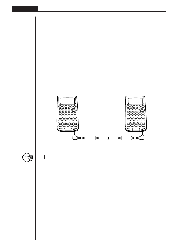
Chapter 9 Data Communications
164
1. Connecting Two Units
The following procedure describes how to connect two units with an optional SB-62
connecting cable for transfer of programs between them.
uu
uu
uTo connect two units
1. Check to make sure that the power of both units is off.
2. Remove the covers from the connectors of the two units.
•Be sure you keep the connector covers in a safe place so you can replace them
after you finish your data communications.
3. Connect the two units using the SB-62 cable.
SB-62 cable
•Keep the connectors covered when you are not using them.
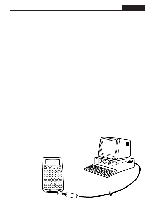
Data Communications Chapter 9
165
2. Connecting the Unit with a
Personal Computer
To transfer data between the unit and a personal computer, you must connect them
through a separately available CASIO Interface Unit.
For details on operation, the types of computer that can be connected, and hardware
limitations, see the user’s guide that comes with the Interface Unit.
Some types of data may not be able to be exchanged with a personal computer.
uu
uu
uTo connect the unit with a personal computer
1. Check to make sure that the power of the unit and the personal computer is off.
2. Connect the personal computer to the Interface Unit.
3. Remove the cover from the connector of the unit.
•Be sure you keep the connector cover in a safe place so you can replace it after
you finish your data communications.
4. Connect the unit to the Interface Unit.
5. Turn on the power of the unit, followed by the personal computer.
•After you finish data communications, turn off power in the sequence: the unit
first, and then the personal computer. Finally, disconnect the equipment.
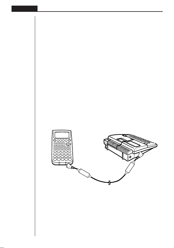
Chapter 9 Data Communications
166
3. Connecting the Unit with a CASIO
Label Printer
After you connect the unit to a CASIO Label Printer with an optional SB-62 cable,
you can use the Label Printer to print screen shot data from the unit. See the user’s
guide that comes with your Label Printer for details on how to perform this operation.
• The operation described above can be performed using the following Label Printer
models: KL-2000, KL-2700, KL-8200, KL-8700 (as of February 2002).
uu
uu
uTo connect the unit with a Label Printer
1. Check to make sure that the power of the unit and the Label Printer is off.
2. Connect the optional SB-62 cable to the Label Printer.
3. Remove the cover from the connector of the unit.
•Be sure you keep the connector cover in a safe place so you can replace it after
you finish your data communications.
4. Connect the other end of the SB-62 cable to the unit.
5. Turn on the power of the unit, followed by the Label Printer.
•After you finish data communications, turn off power in the sequence: the unit
first, and then the Label Printer. Finally, disconnect the equipment.
SB-62 cable
Label Printer
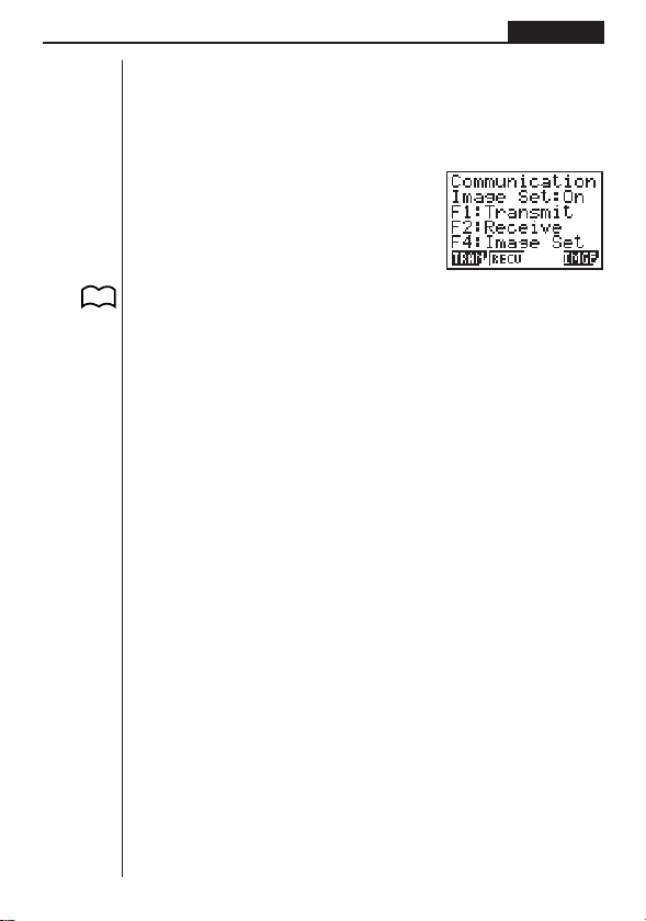
Data Communications Chapter 9
167
4. Before Performing a Data
Communication Operation
In the Main Menu, select the LINK icon and enter the LINK Mode. The following data
communication main menu appears on the display.
Image Set: ........... Indicates the status of the graphic image send features.
Off: Graphic images not sent.
On: Pressing M sends graphic images.
1 (TRAN) ..... Menu of send settings
2 (RECV) ..... Menu of receive settings
4 (IMGE) ...... Menu of graphic image transfer settings
Communication parameters are fixed at the following settings.
•Speed (BPS): 9600 bits per second
• Parity (PARITY): NONE
P. 172
12 4
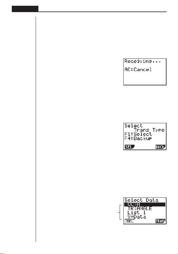
Chapter 9 Data Communications
168
5. Performing a Data Transfer Operation
Connect the two units and then perform the following procedures.
Receiving unit
To set up the calculator to receive data, press 2 (RECV) while the data communi-
cation main menu is displayed.
2(RECV)
The calculator enters a data receive standby mode and waits for data to arrive. Ac-
tual data receive starts as soon as data is sent from the sending unit.
Sending unit
To set up the calculator to send data, press 1 (TRAN) while the data communica-
tion main menu is displayed.
1 (TRAN)
Press the function key that corresponds to the type of data you want to send.
1 (SEL) ........ Selects data items and sends them
4 (BACK) ..... All memory contents, including mode settings
uu
uu
uTo send selected data items
Press 1 (SEL) to display a data item selection screen.
1(SEL)
Data items
1 2 4
1 2 4

Data Communications Chapter 9
169
1 (SEL) ........ Selects data item where cursor is located.
4 (TRAN) ..... Sends selected data items.
Use the f and c cursor keys to move the cursor to the data item you want to
select and press 1 (SEL) to select it. Currently selected data items are marked
with “'”. Pressing 4 (TRAN) sends all the selected data items.
•To deselect a data item, move the cursor to it and press 1 (SEL) again.
Only items that contain data appear on the data item selection screen. If there are
too many data items to fit on a single screen, the list scrolls when you move the
cursor to the bottom line of the items on the screen.
The following types of data items can be sent.
Data Item Contents
Overwrite Password
Check*
1
Check*
2
Program Program contents Yes Yes
List n List memory (1 to 6) contents Yes
Y=Data
Graph expressions, graph write/
non-write status, View Window No
contents, zoom factors
V-WinView Window memory contents No
Variable Variable assignments No
*
1
No overwrite check: If the receiving unit already contains the same type of data, the existing
data is overwritten with the new data.
With overwrite check: If the receiving unit already contains the same type of data, a mes-
sage appears to ask if the existing data should be overwritten with the new data.
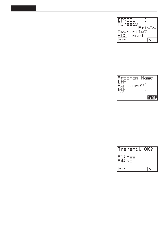
Chapter 9 Data Communications
170
1 (YES) ........ Replaces the receiving unit’s existing data with the new data.
4 (NO) ......... Skips to next data item.
*
2
With password check: If a file is password protected, a message appears asking
for input of the password.
Name of password protected file
Password input field
4 (SYBL)...... Symbol input
After inputting the password, press w.
uu
uu
uTo execute a send operation
After selecting the data items to send, press 4 (TRAN). A message appears to
confirm that you want to execute the send operation.
4(TRAN)
1 (YES) ........ Sends data.
4 (NO) ......... Returns to data selection screen.
Data item name
1 2 4
12 4
1 2 4
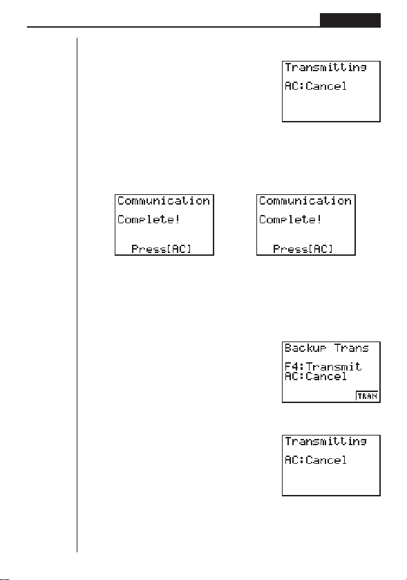
Data Communications Chapter 9
171
Press 1 (YES) to send the data.
1(YES)
•You can interrupt a data operation at any time by pressing A.
The following shows what the displays of the sending and receiving units look like
after the data communication operation is complete.
Sending Unit Receiving Unit
Press A to return to the data communication main menu.
uu
uu
uTo send backup data
This operation allows you to send all memory contents, including mode settings.
While the send data type selection menu is on the screen, press 4 (BACK), and
the back up send menu shown below appears.
4(BACK)
Press 4 (TRAN) to start the send operation.
4(TRAN)
The following shows what the displays of the sending and receiving units look like
after the data communication operation is complete.
12 4
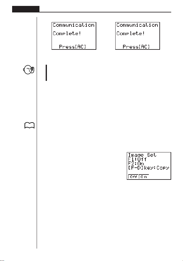
Chapter 9 Data Communications
172
Sending Unit Receiving Unit
Press A to return to the data communication main menu.
•Data can become corrupted, necessitating a RESET of the receiving unit, should
the connecting cable become disconnected during data transfer. Make sure
that the cable is securely connected to both units before performing any data
communication operation.
6. Screen Send Function
The following procedure sends a bit mapped screen shot of the display to a con-
nected computer.
uu
uu
uTo send the screen
1. Connect the unit to a personal computer or to a CASIO Label Printer.
2. In the data communication main menu, press 4 (IMGE), and the following dis-
play appears.
4(IMGE)
1(Off) ........... Graphic images not sent
2(On) ........... Bitmap
3. Display the screen you want to send.
4. Set up the personal computer or Label Printer to receive data. When the other
unit is ready to receive, press M to start the send operation.
P. 165
P. 167
12 4

Data Communications Chapter 9
173
You cannot send the following types of screens to a computer.
• The screen that appears while a data communication operation is in progress.
•A screen that appears while a calculation is in progress.
• The screen that appears following the reset operation.
• The low battery message.
• The flashing cursor is not included in the screen image that is sent from the
unit.
• If you send a screen shot of any of the screens that appear during the data
send operation, you will not be able to then use the sent screen to proceed with
the data send operation. You must exit the data send operation that produced
the screen you sent and restart the send operation before you can send addi-
tional data.
•You cannot use 6mm wide tape to print a screen shot of a graph.
7. Data Communications Precautions
Note the following precautions whenever you perform data communications.
•An error occurs whenever you try to send data to a receiving unit that is not yet
standing by to receive data. When this happens, press A to clear the error and
try again, after setting up the receiving unit to receive data.
•An error occurs whenever the receiving unit does not receive any data approxi-
mately six minutes after it is set up to receive data. When this happens, press A
to clear the error.
•An error occurs during data communications if the cable becomes disconnected,
the parameters of the two units do not match, or if any other communications
problem occurs. When this happens, press A to clear the error, then correct the
problem before trying data communications again. If data communications are
interrupted by the A key operation or an error, any data successfully received
up to the interruption will be in the memory of the receiving unit.
•An error occurs if the receiving unit memory becomes full during data communi-
cations. When this happens, press A to clear the error and delete unneeded
data from the receiving unit to make room for the new data, and then try again.
•To send picture (graph) memory data, the receiving unit need 1-kbytes of memory
for use as a work area in addition to the data being received.

Chapter 9 Data Communications
174

Program Library
1Prime Factor Analysis
2Greatest Common Measure
3
t-Test Value
4Circle and Tangents
5Rotating a Figure
Before using the Program Library
•Be sure to check how many bytes of unused memory are remain-
ing before attempting to perform any programming.
• This Program Library is divided into two sections: a numeric cal-
culation section and a graphics section. Programs in the numeric
calculation section produce results only, while graphics programs
use the entire display area for graphing. Also note that calcula-
tions within graphics programs do not use the multiplication sign
(×) wherever it can be dropped (i.e. in front of open parenthesis).
Chapter
10
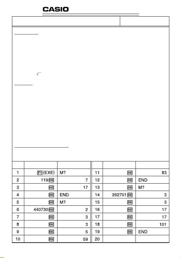
176
PROGRAM SHEET
Program for
Prime Factor Analysis
Description
Produces prime factors of arbitrary positive integers
For 1 <
m < 10
10
Prime numbers are produced from the lowest value first. “END” is displayed at the end
of the program.
(Overview)
m is divided by 2 and by all successive odd numbers (d = 3, 5, 7, 9, 11, 13, ....) to check
for divisibility.
Where
d is a prime factor, mi = mi–1/d is assumed, and division is repeated until
mi + 1 < d.
Example [1]
119 = 7 × 17
[2]
440730 = 2 × 3 × 3 × 5 × 59 × 83
[3]
262701 = 3 × 3 × 17 × 17 × 101
Preparation and operation
•Store the program written on the next page.
•Execute the program as shown below.
Step Key operation Display Step Key operation Display
No.
1
177
1
2
3
4
5
6
7
8
9
10
11
12
13
14
15
16
17
18
19
20
21
22
23
24
25
26
27
P
Lbl
Lbl
Lbl
Lbl
Lbl
Goto
Lbl
Lbl
Lbl
Lbl
Lbl
R
0
1
2
3
4
6
5
6
7
8
9
M
:
:
:
:
:
:
:
:
:
:
:
"
2
Frac
B
B
A
B
A
"
F
M
^
(
A
I
+
÷
^
^
E
A
"
A
A
+
C
2
B
A
N
C
?
÷
÷
1
⇒
→
×
÷
D
T
→
2
2
→
Goto
B
B
B
"
:
A
=
:
:
Goto
A
A
Goto
A
→
)
C
8
:
–
→
^
Goto
:
0
Frac
4
=
:
0
2
A
⇒
(
:
0
Goto
:
=
Goto
A
⇒
3
1
1
÷
Goto
:
⇒
:
B
7
A
B
C
D
E
F
G
H
I
J
K
L
M
N
O
P
Q
R
S
T
U
V
W
X
Y
Z
m
i
d
m
i
+1
Goto
3
)
:
9
→
=
Goto
:
B
0
5
:
⇒
:
No.
1
Line
Program
File
name
Memory Contents
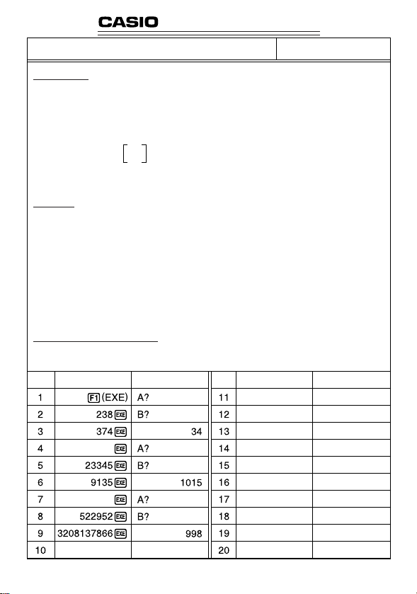
178
PROGRAM SHEET
Program for
Greatest Common Measure
Description
Euclidean general division is used to determine the greatest common measure for two interers
a and b.
For |
a|, |b| < 10
9
, positive values are taken as < 10
10
(Overview)
n0 = max (|a|, |b|)
n1 = min (|a|, |b|)
nk–2
nk = nk–2 – ––– nk–1
nk–1
k = 2, 3....
If
nk = 0, then the greatest common measure (c) will be nk–1.
Example [1] [2] [3]
When
a = 238 a = 23345 a = 522952
b = 374 b = 9135 b = 3208137866
↓↓ ↓
c = 34 c = 1015 c = 998
Preparation and operation
•Store the program written on the next page.
•Execute the program as shown below.
Step Key operation Display Step Key operation Display
No.
2

179
1
2
3
4
5
6
7
8
9
10
11
12
13
14
15
16
17
18
19
20
21
22
23
24
25
26
27
C
Lbl
Abs
B
A
Lbl
C
B
Lbl
M
1
A
<
→
2
=
→
3
N
:
→
A
C
:
0
A
:
"
A
⇒
:
(
–
)
⇒
:
B
F
A
:
Goto
B
(
Goto
C
^
A
"
Abs
2
→
lnt
3
→
Goto
C
?
B
:
A
(
:
B
1
T
→
→
:
A
:
:
:
→
B
2
A
B
C
÷
Goto
"
B
)
:
B
:
×
"
B
?
–
→
A
A
B
C
D
E
F
G
H
I
J
K
L
M
N
O
P
Q
R
S
T
U
V
W
X
Y
Z
a, n
0
b, n
1
n
k
B
)
:
→ C:
No.
2
Line
Program
File
name
Memory Contents
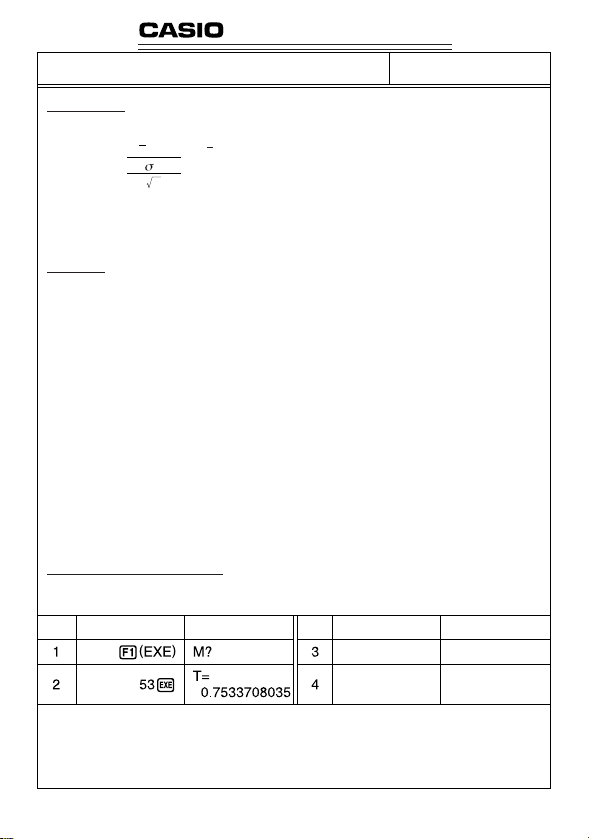
180
Program for
t-Test Value
Description
The mean (sample mean) and sample standard deviation can be used to obtain a t-test value.
x : mean of x data
xσn–1 : sample standard deviation of x data
n : number of data items
m : hypothetical population standard deviation (normally repre-
sented by
µ
, but m is used here because of variable name
limitations)
Example To determine whether the population standard deviation for sample data 55, 54, 51,
55, 53, 53, 54, 52, is 53.
Perform a
t-test with a level of significance of 5%.
Preparation and operation
•Store the program written on the next page.
•Execute the program as shown below.
PROGRAM SHEET
No.
3
Step Key operation Display Step Key operation Display
The above operation produces a t-test value of t(53) = 0.7533708035. According to the t-distribution
table in the next page, a level of significance of 5% and a degree of freedom of 7 (
n – 1 = 8 – 1 = 7)
produce a two-sided
t-test value of approximately 2.365. Since the calculated t-test value is lower
than the table value, the hypothesis that population mean
m equals 53 is accepted.
t =
(x – m)
x
n–1
n
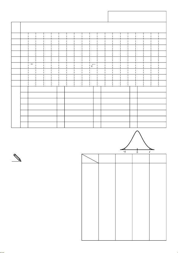
181
1
2
3
4
5
6
7
8
9
10
15
20
25
30
35
40
45
50
60
80
120
240
∞
0.2
3.078
1.886
1.638
1.533
1.476
1.440
1.415
1.397
1.383
1.372
1.341
1.325
1.316
1.310
1.306
1.303
1.301
1.299
1.296
1.292
1.289
1.285
1.282
0.1
6.314
2.920
2.353
2.132
2.015
1.943
1.895
1.860
1.833
1.812
1.753
1.725
1.708
1.697
1.690
1.684
1.679
1.676
1.671
1.664
1.658
1.651
1.645
12.706
4.303
3.182
2.776
2.571
2.447
2.365
2.306
2.262
2.228
2.131
2.086
2.060
2.042
2.030
2.021
2.014
2.009
2.000
1.990
1.980
1.970
1.960
63.657
9.925
5.841
4.604
4.032
3.707
3.499
3.355
3.250
3.169
2.947
2.845
2.787
2.750
2.724
2.704
2.690
2.678
2.660
2.639
2.617
2.596
2.576
0.05 0.01
1
2
3
4
5
6
7
T
{
5
l-Var
Lbl
(
"
Goto
5
4
List
0
x
T
0
T
5
,
1
:
–
=
E
,
5
,
"
M
"
S
5
2
1
M
)
:
T
4
}
_
"
÷
T
,
→
?
(
^
5
List
→
x
σ
n
–1
,
_
_
1
1
M
÷
5
n
5
)
,
→
5
T
3
_
A
B
C
D
E
F
G
H
I
J
K
L
M
N
O
P
Q
R
S
T
U
V
W
X
Y
Z
mt
,53,
P (Probability)
Degree
of Freedom
No.
3
Line
Program
• t-distribution table
The values in the top row of the table show the probability (two-sided
probability) that the absolute value of
t is greater than the table values
for a given degree of freedom.
Memory Contents
File
name
M:aM
T:aT
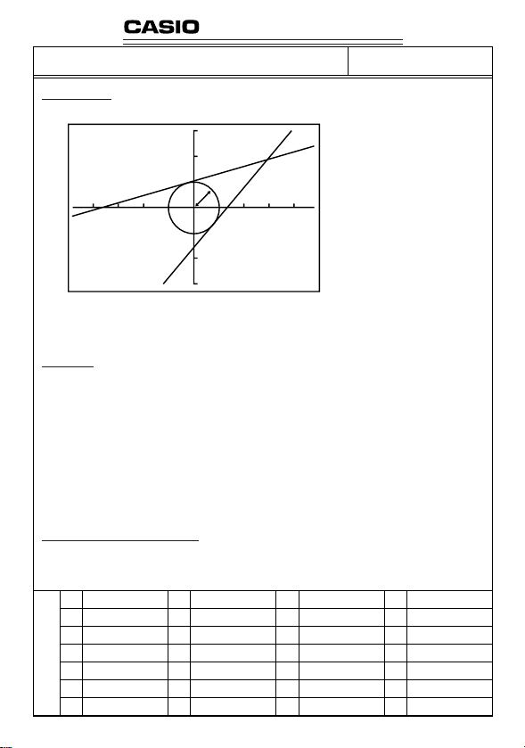
182
PROGRAM SHEET
Program for
Circle and Tangents
Description
Formula for circle:
x
2
+ y
2
= r
2
Formula for tangent line passing
through point A (
x', y'):
y – y' = m (x – x')
*
m represents the slope of the
tangent line
With this program, slope
m and intercept b (= y' – mx') are obtained for lines drawn from point
A (
x', y') and are tangent to a circle with a radius of r. The trace function is used to read out the
coordinates at the points of tangency, and factor zoom is used to enlarge the graph.
Example
To determine m and b for the following values:
r = 1
x' = 3
y' = 2
Notes
• The point plotted for A cannot be moved. Even if it is moved on the graph, the calculation is
performed using the original value.
•An error (Ma ERROR) occurs when
r = x'.
•Be sure to always perform a trace operation whenever you select trace and the message
TRACE is on the display.
Preparation and operation
•Store the program written on the next page.
•Execute the program as shown below.
No.
4
0
X
Y
A
(x',y')
r
A
B
C
D
E
F
G
H
I
J
K
L
M
N
O
P
Q
R
S
T
U
V
W
X
Y
Z
Memory Contents
183
1
2
3
4
5
6
7
8
9
10
11
12
13
14
15
16
17
18
19
20
21
22
23
24
25
26
27
28
29
30
31
32
33
34
T
Prog
"
R
Prog
"
X
"
Plot
R
(
Lbl
Graph Y=
"
"
Lbl
"
Y
N
1
Z
Lbl
(
Graph Y=
"
"
Lbl
"
Y
N
2
Z
Lbl
"
"
A
"
X
=
"
(
=
Y
A
x
2
6
M
M
B
0
T
E
O
→
=
2
(–)
N
M
B
5
T
E
O
→
=
1
T
Factor
N
W
x
2
"
C
X
"
=
,
(
P
_
(
=
=
_
R
S
⇒
S
0
_
A
(
=
=
_
R
S
⇒
S
0
_
R
N
G
I
+
?
I
,
?
"
B
A
–
X
"
"
A
⇒
0
:
⇒
B
X
"
"
A
⇒
0
:
⇒
A
:
E
N
Y
→
R
Y
→
?
^
x
2
A
–
:
:
C
1
"
Z
Goto
–
–
:
:
C
1
"
Z
Goto
C
N
N
D
x
2
R
C
)
A
→
+
B
A
M
B
E
_
:
=
2
A
N
B
E
_
:
=
3
E
=
T
O
=
_
L
_
_
B
B
)
)
^
–
?
?
1
:
P
)
^
–
?
?
1
:
"
"
W
R
E
_
x
2
(
+
M
_
→
⇒
Goto
)
+
N
_
→
⇒
Goto
^
?
_
_
^
R
x
2
^
^
_
1
_
R
^
^
_
1
_
F
"
x
2
"
–
R
B
A
Z
Goto
0
(
B
A
Z
Goto
5
→
x
2
–
)
A
→
x
2
P
)
_
x
–1
_
_
:
x
2
–
Factor
A
F
x
2
_
)
→
x
–1
M
→
_
N
_
No.
4
Line
Program
File
name

184
View
Window
35
36
37
38
39
40
41
42
43
44
1
2
1
2
Prog
S
Graph Y=
Goto
Lbl
Graph Y=
Prog
:
Lbl
"
W
3
C
Graph Y=
Graph Y=
"
=
N
3
9
M
"
Goto
3
E
I
(–)
,
I
(–)
C
2
(
_
_
(
W
6
_
N
N
3
1
R
(
I
⇒
X
X
I
_
D
D
.
C
R
(
R
Graph Y=
–
–
N
"
O
9
L
x
2
R
C
M
A
A
D
W
,
E
–
x
2
L
(
)
)
O
3
X
–
E
X
+
+
W
.
x
2
X
:
A
^
^
:
,
_
)
"
–
B
B
"
9
)
x
2
S
)
Prog
1
=
+
"
,
1
B
C
(–)
⇒
_
I
2
Goto
R
.
9
C
3
_
L
,
E
2
"
.
No.
4
Line
Program
File
name
File
name
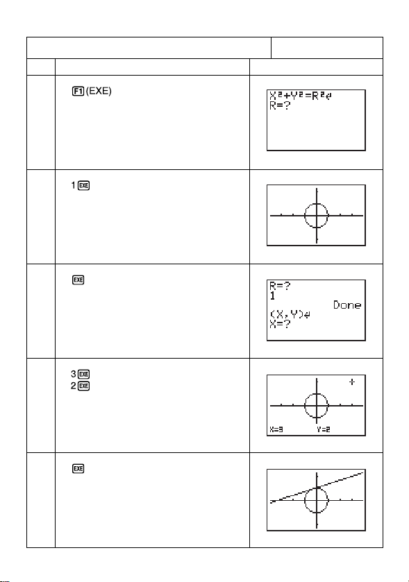
185
1
2
3
4
5
Program for
Circle and Tangents
No.
4
Step Key Operation Display
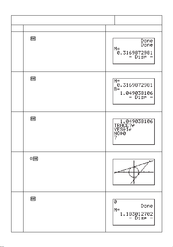
186
Program for
Circle and Tangents
No.
4
Step Key Operation Display
6
7
8
9
10
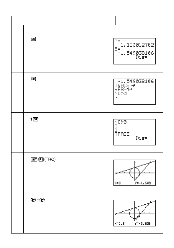
187
11
12
13
14
15
Program for
Circle and Tangents
No.
4
Step Key Operation Display

188
16
17
18
Program for
Circle and Tangents
No.
4
Step Key Operation Display
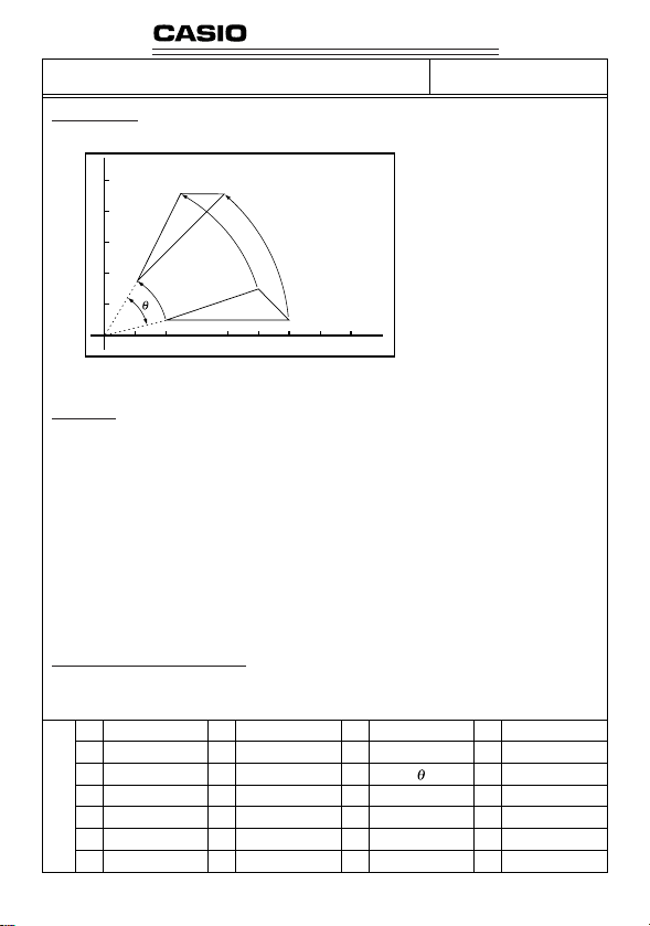
189
PROGRAM SHEET
Program for
Rotating a Figure
Description
Formula for coordinate transforma-
tion:
(
x, y) → (x', y')
x' = x cos
θ
– y sin
θ
y' = x sin
θ
+ y cos
θ
Graphing of rotation of any geometric figure by
θ
degrees.
Example
To r o tate by 30° the triangle defined by points A (2, 0.5), B (6, 0.5), and C (5, 1.5)
Notes
•Use the cursor keys to move the pointer around the display.
•To interrupt program execution, press A while the graphic screen is on the display.
• The triangle cannot be drawn if the result of the coordinate transformation operation exceeds
View Window parameters.
Preparation and operation
•Store the program written on the next page.
•Execute the program as shown below.
No.
5
Memory Contents
A
B
C
D
E
F
G
x
1
y
1
x
2
y
2
x
3
y
3
x'
1
y'
1
x'
2
y'
2
x'
3
y'
3
H
I
J
K
L
M
N
O
P
Q
R
S
T
U
V
W
X
Y
Z
0
X
Y
B(x
2,
y
2
)
A(x
1,
y
1
)
C(x
3,
y
3
)

190
No.
5
Line
Program
File
name
1
2
3
4
5
6
7
8
9
10
11
12
13
14
15
16
17
18
19
20
21
22
23
24
25
26
27
28
29
30
31
32
33
34
R
8
"
X
"
Plot
X
"
X
"
Plot
X
"
X
"
Plot
X
Lbl
Line
"
A
A
Plot
C
C
Plot
E
E
Plot
Plot
Cls
O
(–)
,
(
1
Y
A
→
(
2
Y
C
→
(
3
Y
E
→
1
:
A
cos
sin
G
cos
sin
I
cos
sin
K
G
:
T
0
1
X
=
1
,
A
X
=
2
,
C
X
=
3
,
E
_
Plot
N
Q
Q
,
Q
Q
,
Q
Q
,
,
Plot
A
.
:
1
"
=
B
:
2
"
=
D
:
3
"
=
F
:
A
G
–
+
H
–
+
J
–
+
L
H
C
T
4
Deg
,
?
"
^
Y
,
?
"
^
Y
,
?
"
^
Y
,
L
B
B
_
D
D
:
F
F
:
:
,
E
,
_
Y
→
?
→
Y
→
?
→
Y
→
?
→
B
E
sin
cos
sin
cos
Line
sin
cos
Line
Line
D
7
1
A
→
B
2
C
→
D
3
E
→
F
:
:
Q
Q
Q
Q
_
Q
Q
_
^
:
.
)
_
B
_
)
_
D
_
)
_
F
_
Line
Deg
→
→
→
→
→
→
Plot
,
Plot
?
_
_
_
_
_
_
,
4
_
_
_
_
_
_
:
"
G
H
I
J
K
L
E
1
C
→
,
,
Q
(–)
D
_
0
:
.
Line
F
View
Window
:
Goto
1
8,3.
^
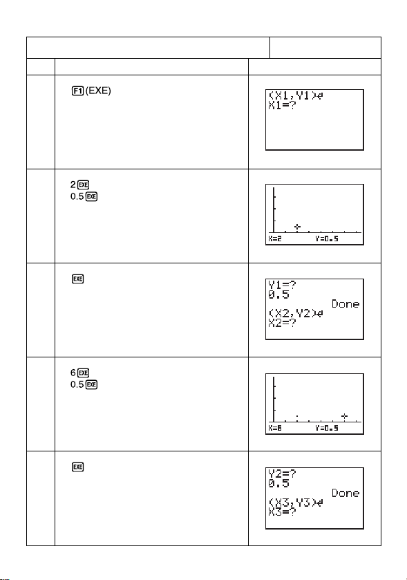
191
1
2
3
4
5
Program for
Rotating a Figure
No.
5
Step Key Operation Display
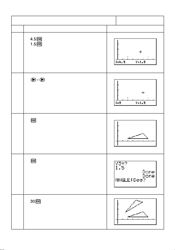
192
6
7
8
9
10
Program for
Rotating a Figure
No.
5
Step Key Operation Display
(Locate the pointer at X = 5)
Continue, repeating from step 8.

Appendix
Appendix A Resetting the Calculator
Appendix B Power Supply
Appendix C Error Message Table
Appendix D Input Ranges
Appendix E Specifications
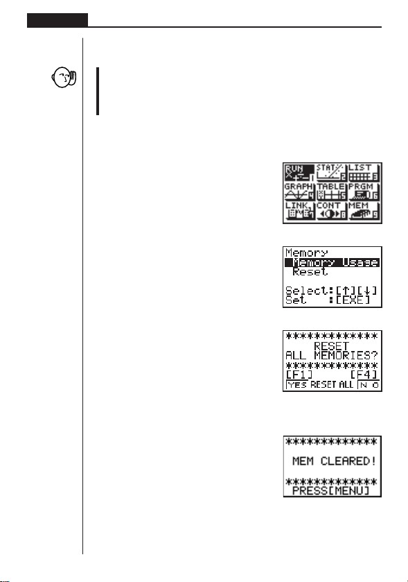
194
Appendix
Appendix A Resetting the Calculator
Warning!
The procedure described here clears all memory contents. Never perform this op-
eration unless you want to totally clear the memory of the calculator. If you need
the data currently stored in memory, be sure to write it down somewhere before
performing the RESET operation.
uu
uu
uTo reset the calculator
1. Press m to display the main menu.
2. Highlight the MEM icon and press w, or press j.
3. Use c to move the highlighting down to “Reset” and then press w.
4. Press 1 (YES) to reset the calculator or 4 (NO) to abort the operation without
resetting anything.
• If the display appears to dark or dim after you reset the calculator, adjust contrast.
1 234

195
Appendix
Resetting the calculator initializes it to the following settings.
Item Initial Setting
Icon RUN
Angle Unit Rad
Exponent Display Range Norm 1
Fraction Reduction Automatic
Mixed Fraction Display
Graph Type Rectangular coordinate (Y=)
Statistical Graph Automatic
Va r i able Memory Clear
Answer Memory (Ans) Clear
Graphic Display/Text Display Clear
View Window Clear (initialized)
View Window Memory Clear
Graph Function Clear
Enlargement/Reduction Factor Clear (initialized)
Table & Graph Data Clear
List Data Clear
Statistical Calculation/Graph Memory Clear
Program Clear
Input Buffer/AC Replay Clear
•Performing the RESET operation while an internal calculation is being per-
formed will cause all data in memory to be deleted. Make sure that no calcula-
tion be being performed before starting a RESET operation.
• If the calculator stops operating correctly for some reason, use a thin, pointed
object to press the P button on the back of the calculator. This should make the
RESET confirmation screen appear on the display. Perform the procedure to
complete the RESET operation.
P button
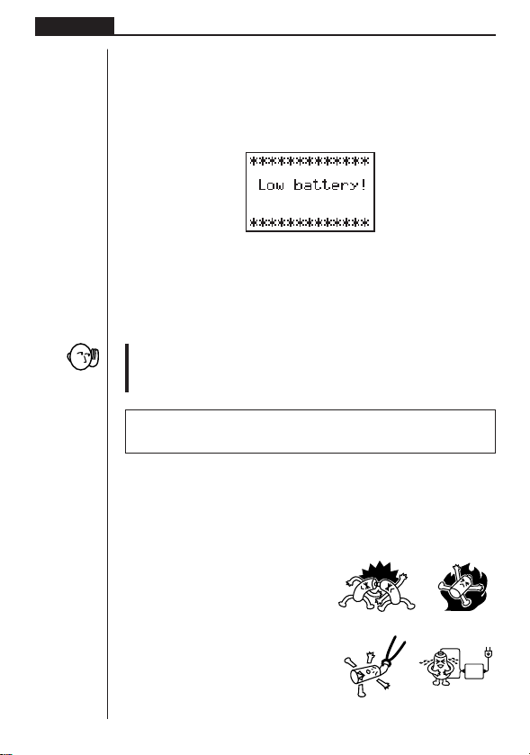
196
Appendix
Appendix B Power Supply
This unit is powered by two AAA-size (LR03 (AM4) or R03 (UM-4)) batteries. In addi-
tion, it uses a single CR2032 lithium battery as a back up power supply for the memory.
If the following message appears on the display, immediately stop using the calcula-
tor and replace batteries.
If you try to continue using the calculator, it will automatically switch power off, in
order to protect memory contents. You will not be able to switch power back on until
you replace batteries.
Be sure to replace the main batteries at least once every two years, no matter how
much you use the calculator during that time.
Warning!
If you remove both the main power supply and the memory back up batteries at the
same time, all memory contents will be erased. If you do remove both batteries,
correctly reload them and then perform the reset operation.
The batteries that come with this unit discharge slightly during shipment and
storage. Because of this, they may require replacement sooner than the normal
expected battery life.
kk
kk
k Replacing Batteries
Precautions:
Incorrectly using batteries can cause them to burst or leak, possibly damaging the
interior of the unit. Note the following precautions:
•Be sure that the positive (+) and negative (–) poles of each battery are facing in
the proper directions.
•Never mix batteries of different types.
•Never mix old batteries and new ones.
•Never leave dead batteries in the battery
compartment.
•Remove the batteries if you do not plan to
use the unit for long periods.
•Never try to recharge the batteries sup-
plied with the unit.
•Do not expose batteries to direct heat, let
them become shorted, or try to take them
apart.
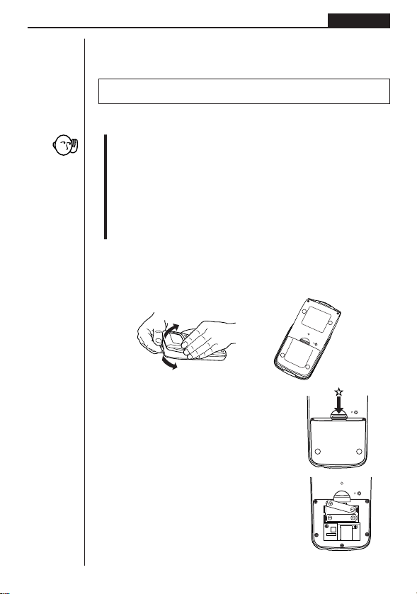
197
Appendix
(Should a battery leak, clean out the battery compartment of the unit immedi-
ately, taking care to avoid letting the battery fluid come into direct contact with
your skin.)
Keep batteries out of the reach of small children. If swallowed, consult with a
physician immediately.
uu
uu
uTo replace the main power supply batteries
*Never remove the main power supply and the memory back up batteries from
the unit at the same time.
*Be sure to switch the unit off before replacing batteries. Replacing batteries
with power on will cause data in memory to be deleted.
*Never replace the back cover or switch the calculator on while the main power
supply batteries are removed from the calculator or not loaded correctly. Doing
so can cause memory data to be deleted and malfunction of the calculator. If
mishandling of batteries causes such problems, correctly load batteries and
then perform the RESET operation to resume normal operation.
*Be sure to replace all two batteries with new ones.
1. Press !O to turn the calculator off.
2. Making sure that you do not accidently press the o key, attach the case to the
calculator and then turn the calculator over.
3. Remove the back cover from the unit by pull-
ing with your finger at the point marked
✩.
4. Remove the two old batteries.
5. Load a new set of two batteries, making sure
that their positive (+) and negative (–) ends
are facing in the proper directions.
6. Replace the back cover and press o to turn
power on. The memory back-up battery pro-
vides power to the memory while the main
batteries are removed, so memory data is not
lost.
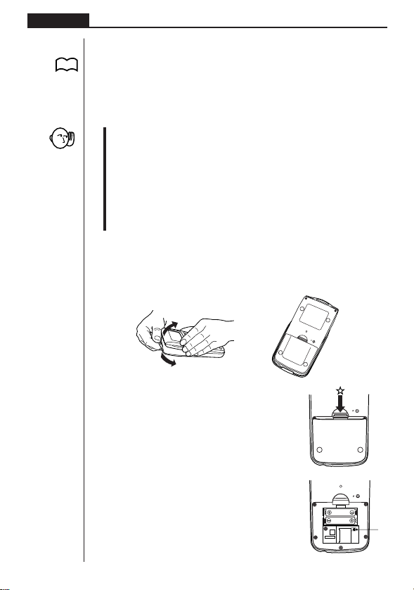
198
Appendix
•Power will not switch on if you press o while the back cover is open.
•Do not leave the unit without main power supply batteries loaded for long periods.
Doing so can cause deletion of data stored in memory.
• If the figures on the display appear too light and hard to see after you turn on
power, adjust the contrast.
uu
uu
uTo replace the memory back up battery
*Before replacing the memory back up battery, switch on the unit and check to see
if the “Low battery!” message appears on the display. If it does, replace the main
power supply batteries before replacing the back up power supply battery.
* Never remove the main power supply and the memory back up batteries from the
unit at the same time.
*Be sure to switch the unit off before replacing battery. Replacing battery with
power on will cause data in memory to be deleted.
*Be sure to replace the back up power supply battery at least once 2 years, re-
gardless of how much you use the unit during that time. Failure to do so can
cause data in memory to be deleted.
1. Press !O to turn the calculator off
2. Making sure that you do not accidently press the o key, attach the case to the
calculator and then turn the calculator over.
i
3. Remove the back cover from the unit by pull-
ing with your finger at the point marked
✩.
4. Remove screw
i
on the back of the calcula-
tor, and remove the back up battery holder.
5. Remove the old battery.
P. 11

199
Appendix
6. Wipe off the surfaces of a new battery with a
soft, dry cloth. Load it into the calculator so
that its positive (+) side is facing up.
7. Pressing down on the battery with the battery
holder, replace the screw that secures the
holder in place.
8. Replace the back cover and press o to turn power on. The main batteries
provide power to the memory while the back-up battery is removed, so memory
data is not lost.
kk
kk
k About the Auto Power Off Function
The calculator switches power off automatically if you do not perform any key opera-
tion for about 6 minutes. To restore power, press o.
The calculator automatically turns off it is left for about 60 minutes with a calculation
stopped by an output command (^), which is indicated by the “–Disp–” message on
the display.

200
Appendix
Meaning
1 Calculation formula contains an
error.
2 Formula in a program contains
an error.
1 Calculation result exceeds
calculation range.
2 Calculation is outside the input
range of a function.
3 Illogical operation (division by
zero, etc.)
4 Poor precision in differential
calculation results.
1 No corresponding Lbl
n for
Goto
n.
2 No program stored in program
area Prog “file name”.
3 No corresponding “Next” for
“For”, no corresponding
“LpWhile” for “Do”, or no
corresponding “WhileEnd” for
“While”.
•Nesting of subroutines exceeds
10 levels.
Countermeasure
1 Use d or e to display the
point where the error was
generated and correct it.
2 Use d or e to display the point
where the error was generated
and then correct the program.
123
Check the input numeric value
and correct it.
When using memories, check
that the numeric values stored
in memories are correct.
4 Try using a smaller value for ∆
x
(x increment/decrement).
1 Correctly input a Lbl
n to corres-
pond to the Goto
n , or delete
the Goto
n if not required.
2 Store a program in program
area Prog “file name”, or delete
the Prog “file name” if not
required.
3 Correctly match “Next” with
“For”, “LpWhile” with “Do”, or
“WhileEnd” with “While”.
•Ensure that Prog “file name” is
not used to return from
subroutines to main routine. If
used, delete any unnecessary
Prog “file name”.
• Trace the subroutine jump
destinations and ensure that no
jumps are made back to the
original program area. Ensure
that returns are made correctly.
Appendix C Error Message Table
Message
Syn ERROR
Ma ERROR
Go ERROR
Ne ERROR

201
Appendix
Meaning
•Execution of calculations that
exceed the capacity of the stack
for numeric values or stack for
commands.
1 Not enough memory to hold
function input in the Graph
Mode for graph drawing.
2 Not enough memory to hold
function input in the TABLE
Mode.
3 Not enough memory to store
data in list function.
•Incorrect argument specification
for a command that requires an
argument.
• Illegal dimension used during
list calculations.
•Problem with cable connection
or parameter setting during
program data communications.
•Problem with cable connection
or parameter setting during
data communications.
•Problem with cable connection
or parameter setting during
data communications.
•Memory of receiving unit
became full during program
data communications.
Countermeasure
•Simplify the formulas to keep
stacks within 10 levels for the
numeric values and 26 levels
for the commands.
•Divide the formula into two or
more parts.
123
•Keep the number of variables
you use for the operation within
the number of variables
currently available.
•Simplify the data you are trying
to store to keep it within the
available memory capacity.
•Delete no longer needed data
to make room for the new data.
Correct the argument.
•Fix
n, Sci n : n = integer from 0
through 9.
• Lbl
n , Goto n : n = integer from
0 through 9.
•Check list dimension.
•Check cable connection.
•Check cable connection.
•Check cable connection.
•Delete some data stored in the
receiving unit and try again.
Message
Stk ERROR
Mem ERROR
Arg ERROR
Dim ERROR
Com ERROR
Transmit
ERROR!
Receive ERROR!
Memory Full!

202
Appendix
Function
sin
x
cosx
tanx
sin
–1
x
cos
–1
x
tan
–1
x
logx
Inx
10
x
e
x
x
x
2
1/x
3
x
x
!
nPr
n
Cr
Pol (x, y)
Rec
(
r ,
θ
)
Internal
digits
15 digits
"
"
"
"
"
"
"
"
"
Precision
As a rule,
precision is
±1 at the
10th digit.
*
"
"
"
"
"
"
"
"
"
Notes
However, for tan
x:
|
x|
GG
GG
G
90(2n+1):DEG
|
x|
GG
GG
G
π/2(2n+1):RAD
|
x|
GG
GG
G
100(2n+1):GRA
Input ranges
(DEG) |
x| < 9 × 10
9
°
(RAD) |
x| < 5 × 10
7
πrad
(GRA) |
x| < 1 × 10
10
grad
|
x| < 1
|
x| < 1 × 10
100
1 × 10
–99
< x < 1 × 10
100
–1 × 10
100
< x < 100
–1 × 10
100
< x < 230.2585092
0 <
x < 1 × 10
100
|x| <1 × 10
50
|x| < 1 × 10
100
, x
GG
GG
G
0
|
x| < 1 × 10
100
0 < x < 69
(
x is an integer)
Result < 1 × 10
100
n, r (n and r are integers)
0 <
r < n,
n < 1 × 10
10
< 1 × 10
100
x
2
+ y
2
|r| < 1 × 10
100
(DEG) |
θ
| < 9 × 10
9
°
(RAD) |
θ
| < 5 × 10
7
π rad
(GRA) |
θ
| < 1 × 10
10
grad
Appendix D Input Ranges
However, for tan
θ
:
|
θ
|
GG
GG
G
90(2n+1):DEG
|
θ
|
GG
GG
G
π/2(2n+1):RAD
|
θ
|
GG
GG
G
100(2n+1):GRA

203
Appendix
Internal
digits
15 digits
"
"
"
"
Precision
As a rule,
precision is
±1 at the
10th digit.
*
"
"
"
"
Notes
Input ranges
|
a|, b, c < 1 × 10
100
0 < b, c
|x| < 1 × 10
100
Sexagesimal display:
|
x| < 1 × 10
7
x > 0:
–1 × 10
100
< y logx < 100
x = 0 : y > 0
x < 0 :
y = n,
(n is an integer)
However;
–1 × 10
100
< y log |x| < 100
y > 0 : x
GG
GG
G
0
–1 × 10
100
< logy < 100
y = 0 : x > 0
y < 0 : x = 2n +1,
(
n
GG
GG
G
0, n is an integer)
However;
–1 × 10
100
< log |y| < 100
To tal of integer, numerator
and denominator must be
within 10 digits (includes di-
vision marks).
|
x| < 1 × 10
50
|y| < 1 × 10
50
|n| < 1 × 10
100
x
σ
n, y
σ
n, x, y, a, b, c, r :
n
GG
GG
G
0
x
σ
n–1, y
σ
n–1: n
GG
GG
G
0, 1
1
–––––
2
n+1
1
––
x
1
––
n
1
––
x
Function
° ’ ”
←
° ’ ”
^(
x
y
)
x
y
a
b
/c
STAT
* For a single calculation, calculation error is ±1 at the 10th digit. (In the case of exponential display,
calculation error is ±1 at the last significant digit.) Errors are cumulative in the case of consecutive
calculations, which can also cause them to become large. (This is also true of internal consecutive
calculations that are performed in the case of ^(
x
y
),
x
y, x!,
3
, nPr, nCr, etc.)
In the vicinity of a function’s singular point and point of inflection, errors are cumulative and may
become large.

204
Appendix
Appendix E Specifications
Variables: 26
Calculation range:
±1 × 10
–99
to ±9.999999999 × 10
99
and 0. Internal operations use 15-digit mantissa.
Exponential display range: Norm 1: 10
–2
> |x|, |x| > 10
10
Norm 2: 10
–9
> |x|, |x| > 10
10
Program capacity:
20,000 bytes (max.)
Power supply:
Main: Two AAA-size batteries (LR03 (AM4) or R03 (UM-4))
Back-up: One CR2032 lithium battery
Power consumption: 0.05W
Battery life
Main:
LR03 (AM4): Approximately 1,500 hours (continuous display of main menu)
Approximately 700 hours (continuous operation)
R03 (UM-4): Approximately 900 hours (continuous display of main menu)
Approximately 400 hours (continuous operation)
Back-up: Approximately 2 years (when main batteries are not supplying power)
Auto power off:
Power is automatically turned off approximately six minutes after last operation.
The calculator automatically turns off if it is left for about 60 minutes with a calcula-
tion stopped by an output command (^), which is indicated by the “–Disp–” mes-
sage on the display.
Ambient temperature range: 0°C to 40°C
Dimensions: 23 mm (H) × 85.5 mm (W) × 169 mm (D)
15
/16" (H) × 3
7
/16" (W) × 6
3
/4" (D)
Weight: 185g (including batteries)
Data Communications
Functions:
Program contents and file names; function memory data; list data; variable data;
Table & Graph data; graph functions
Method: Start-stop (asynchronous), half-duplex
Transmission speed (BPS): 9600 bits/second
Parity: none
Bit length: 8 bits
Stop bit:
Send: 2 bits
Receive: 1 bit

IBM is a registered trademark of International Business Machines Corporation.
Macintosh is a registered trademark of Apple Computer, Inc.
GUIDELINES LAID DOWN BY FCC RULES FOR USE OF THE UNIT IN THE U.S.A. (not appli-
cable to other areas).
NOTICE
This equipment has been tested and found to comply with the limits for a Class B digital device,
pursuant to Part 15 of the FCC Rules. These limits are designed to provide reasonable protec-
tion against harmful interference in a residential installation. This equipment generates, uses
and can radiate radio frequency energy and, if not installed and used in accordance with the
instructions, may cause harmful interference to radio communications. However, there is no guar-
antee that interference will not occur in a particular installation. If this equipment does cause
harmful interference to radio or television reception, which can be determined by turning the
equipment off and on, the user is encouraged to try to correct the interference by one or more of
the following measures:
•Reorient or relocate the receiving antenna.
•Increase the separation between the equipment and receiver.
•Connect the equipment into an outlet on a circuit different from that to which the receiver is
connected.
•Consult the dealer or an experienced radio/TV technician for help.
FCC WARNING
Changes or modifications not expressly approved by the party responsible for compliance could
void the user’s authority to operate the equipment.
Proper connectors must be used for connection to host computer and/or peripherals in order to
meet FCC emission limits.
Connector SB-62 Power Graphic Unit to Power Graphic Unit
Connector FA-123 Power Graphic Unit to PC for IBM/Macintosh Machine
Program Mode Command List
MENU
[OPTN]key
STAT
LIST
DRAW
List List_
On DrawOn
Off DrawOff
Dim Dim_
[PRGM]key
[VARS]key
GRPH
Fill Fill(
COM
V-WIN
GPH1 S-Gph1_
Seq Seq(
If If_
Xmin Xmin
GPH2 S-Gph2_
Then Then_
Xmax Xmax
GPH3 S-Gph3_
Min Min(
Else Else_
Xscl Xscl
Scat Scatter
Max Max(
I·End IfEnd
FACT
xy xyLine
Pie Pie
Stck StackedBar
Mean Mean(
Xfct Xfct
Med Median(
For For_
Yfct Yfct
Hist Hist
To _To_
STAT
Box MedBox
Sum Sum_
Step _Step_
X
N-Dis N-Dist
CALC
Next Next
n n
Simp Simp
oo
Int÷
_Int÷_
W
·
End
While_
Σx Σx
X Linear
Rmdr _Rmdr_
Whle
WhileEnd
Σx2 Σx2
Med Med-Med
STAT
Do Do
xσn xσn
X^2 Quad
x^ x^
Lp·W LpWhile_
y^ y^
CTL
xσn-1 x σn-1
Log Log
Prog Prog_
minX minX
Exp Exp
PROB
Rtrn Return
maxX maxX
Pwr Power
Bar Bar
Line LineG
Both Both
X! !
Brk Break
Y
LIST
nPr P
Stop Stop
pp
List1 List1
nCr C
Σy Σy
List2 List2
Ran# Ran#
JUMP
Σy2 Σy2
List3 List3
NUM
Lbl Lbl_
Σxy Σxy
List4 List4
Abs Abs_
Goto Goto_
yσn yσn
List5 List5
Int Int_
⇒⇒
List6 List6
Frac Frac_
Isz Isz_
yσn-1 y σn-1
MARK
Rnd Rnd
Dsz Dsz_
minY minY
Square
Intg Intg_
? ?
maxY maxY
× Cross
ANGL
^^
GRPH
• Dot
o o
a a
CALC
r r
CLR
b b
1VAR 1-Variable_
g g
Text ClrText
c c
2VAR 2-Variable_
o'''
Grph ClrGraph
List ClrList
r r
X LinearReg_
Pol( Pol(
DISP
Q1 Q1
Med Med-MedLine_
Rec( Rec(
Stat DrawStat
Med Med
X^2 QuadReg_
Grph DrawGraph
Q3 Q3
TABL
Mod Mod
Log LogReg_
Tabl DispTable
PTS
Exp ExpReg_
G-Con DrawTG-Con
x1 x1
Pwr PowerReg_
G-Plt DrawTG-Plt
y1 y1
LIST
REL
I/O
::
x2 x2
SRT-A SortA(
= =
SRT-D SortD(
%
Data
≠≠
y2 y2
GRPH
> >
x3 x3
SEL
DISP
%
Data
Sep
.
G
O
.
Lap
WIN
Sep.G
NormWin
Norm
O
.
Lap
< <
y3 y3
On G_SelOn_
>>
GRPH
Off G_SelOff_
<<
Send Send
(
Recv Receive(
Y Y
TYPE
Xt Xt
Y= Y=Type
Yt Yt
Parm ParamType
TABL
Strt F_Start
Y> Y>Type
End F_End
Y< Y<Type
pitch F_pitch
Y> Y >Type
Y< Y <Type
TABL
[SETUP]key
On T_SelOn_
Off T_SelOff_
Deg
Deg
[SHIFT]key
Rad
Rad
ZOOM
' '
Gra
Gra
Fact Factor_
" "
V-WIN
~ ~
V-Win ViewWindow_
* *
Sto StoV-Win
/ /
Rcl RclV-Win
# #
SKTCH
Fix
Fix_
Cls Cls
Sci
Sci_
GRPH
Norm
Norm
Y= Graph_Y=
Parm Graph(X,Y)=(
Auto
S-WindAuto
Y> Graph_Y>
Man
S-WindMan
Y< Graph_Y<
Rang VarRange
Y> Graph_Y >
List1
VarList1
Y< Graph_Y <
List2
VarList2
List3
VarList3
Plot
PLOT
LINE
Plot
P-On PlotOn
P-Off PlotOff
P-Chg PlotChg
[ALPHA]key
List4
VarList4
Line Line
F-Lin F-Line
' '
List5
VarList5
" ”
List6
VarList6
Hztl Horizontal_
Vert Vertical_
~ ~
d/dx d/dx(
Con
G-Connect
Plot
G-Plot
Ymin Ymin
Ymax Ymax
Yscl Yscl
Tmin Tmin
Tmax Tmax
Tpth Tptch
CASIO ELECTRONICS CO., LTD.
Unit 6, 1000 North Circular Road,
London NW2 7JD, U.K.
Important!
Please keep your manual and all information handy
for future reference.
Declaration of Conformity
Model Number: fx-7400G PLUS
Trade Name: CASIO COMPUTER CO., LTD.
Responsible party: CASIO, INC.
Address: 570 MT. PLEASANT AVENUE, DOVER, NEW JERSEY 07801
Telephone number: 973-361-5400
This device complies with Part 15 of the FCC Rules. Operation is subject to the following two
conditions: (1) This device may not cause harmful interference, and (2) this device must accept
any interference received, including interference that may cause undesired operation.

SA0212-A Printed in China
fx-7400G PLUS
User’s Guide
CASIO COMPUTER CO., LTD.
6-2, Hon-machi 1-chome
Shibuya-ku, Tokyo 151-8543, Japan
E
fx-7400G PLUS (English) Cover Black
fx-7400G PLUS
User’s Guide
E
http://world.casio.com/edu_e/
RCA500487-1